Assessment of thermal stabilization measures based on numerical simulations at a Swiss alpine permafrost site

Global warming causes thawing of permafrost, leading to landscape changes and infrastructure damage, problems that have intensified worldwide in all permafrost regions. This study numerically investigates the impact of different thermal stabilization methods on preventing or delaying permafrost thawing. To test different technical methods, an alpine mountain permafrost site with nearby infrastructure is investigated. Model simulations represent the one-dimensional (1D) effect of heat fluxes across the complex system of snow–ice–permafrost layers and the impact of passive and active cooling, including engineered energy flux dynamics at the surface. The results show the efficiency of different passive, active and combined thermal stabilization methods in influencing heat transfer, temperature distribution, and the seasonal active-layer thickness (ALT). Investigating each component of thermal stabilization helps quantify the efficiency of each method and determine their optimal combination. Despite providing efficient cooling in winter, passive methods are less efficient, as the ALT remains over 1 m. Conductive heat flux attenuation alone takes several years to form a stable frozen layer. Active cooling, when powered by solar energy, decreases the ALT to only a few decimetres. The combination of active and passive cooling, together with conductive heat flux attenuation, performs best and allows excess energy to be fed into the local grid. The findings of this study show the evolution of ground temperature and permafrost at a representative alpine site under natural and thermally stabilized conditions, contributing to understanding the potential and limitations of stabilization systems and formulating recommendations for optimal application.

1 Introduction

The effect of increasing air temperature on permafrost is the result of complex and interacting processes occurring in different layers, including the grain size of rocks, the snow cover, and the active layer. On the continental scale, between 2007 and 2016, the Arctic continuous permafrost experienced a warming of approximately 0.39 °C, while the discontinuous permafrost warmed 0.20 °C (Biskaborn et al., 2019). In particular, this warming reached 0.8 °C per decade in the Svalbard archipelago and 0.5 °C per decade in Russia (Smith et al., 2022). In the same period, global mountain permafrost temperatures increased by 0.19 °C (Biskaborn et al., 2019; Etzelmüller et al., 2020), responding to the rise of the atmospheric 0 °C isotherm (Kenner et al., 2024). The general trend at some alpine mountain permafrost sites showed that warming at 10 m depth was 0.4 °C per decade between 1987 and 2009 (Haeberli and Gruber, 2009; Noetzli et al., 2024). These changes have led to an increase in active-layer thickness (ALT) and shifted latitudinal permafrost limits northward (Biskaborn et al., 2019; Smith et al., 2022) and elevation limits to higher altitudes (Kenner et al., 2024; Noetzli et al., 2024). In Sweden, Greenland, and Svalbard, the ALT has been increasing since the 1990s (Strand et al., 2021), and similarly in mountain permafrost, where it has doubled in parts of the Swiss Alps in the twenty-first century (Smith et al., 2022; Swiss Permafrost Monitoring Network (PERMOS), 2024; Noetzli et al., 2024). On the Schilthorn mountain (Bernese Alps, Switzerland), annual average ground temperatures increased from −0.5 to +0.03 °C, resulting in a tripling of the ALT (Hauck, 2002; Swiss Permafrost Monitoring Network (PERMOS), 2024), while at the Stockhorn borehole (Valais, Switzerland), a four-fold acceleration in warming led to a decadal rate of +0.64 °C between 2012 and 2022 (Morard et al., 2024). At the Murtèl–Corvatsch borehole (Grisons, Switzerland), the warming over 18 years (1987–2006) reached approximately 0.5 °C at 11.6 m depth and 0.3 °C at 21.6 m depth (Harris et al., 2009), with continued increases over 35 years (1987–2022) from −1.8 to −1.0 °C at 15–20 m depth (Haeberli et al., 2023).

Thawing and warming permafrost and increasing ALT present a risk to infrastructure foundations. It has been estimated that almost 70 % of infrastructure in the permafrost could be affected by 2050, with transport infrastructure (roads, railways, cable cars, etc.) being the most vulnerable and most abundant (Hjort et al., 2018, 2022). A prominent Arctic example of infrastructure affected by permafrost changes is the runway of the international airport in Longyearbyen, Svalbard, where the thawing of ice-rich soils caused uneven settlement during the summer season, and the refreezing in the autumn provoked heave formation, ultimately leading to the destruction of the runway (Instanes and Mjureke, 2005). In addition to transport infrastructure, over 1000 settlements, and over 9000 km of pipelines are located in areas subject to permafrost risk (Hjort et al., 2022).

In mountain regions such as the Swiss Alps, permafrost thawing also causes significant impacts. Unlike Arctic areas, mountain permafrost in steep rock slopes contains little ice; its thawing allows water infiltration, which can lead to high pressures and rapid temperature increases. Infrastructure such as cable cars, houses, antennas, and avalanche protection systems built on permafrost rock slopes can be destabilized (Duvillard et al., 2021). An impressive example is the 2017 Pizzo Cengalo rock avalanche in Bondo, Switzerland (Mergili et al., 2020), a cascading event involving rockfall, rock-ice avalanche, and debris flow (Walter et al., 2020). Such process chains are often linked to cryospheric changes such as glacial de-buttressing, retreating hanging glaciers, or thawing permafrost (Harris et al., 2009; Haeberli et al., 2017). Ice-rich permafrost can also develop at the base of steep slopes in the snow avalanche and rockfall deposition zones (Kenner et al., 2019). Although these zones should be avoided in infrastructure planning (Bommer et al., 2010), this is not always possible. Ice warming and melting, combined with water infiltration, can lead to subsidence and creep, damaging the infrastructure on ice-rich ground.

All of these challenges, whether from new or intensifying natural hazards or from the difficulties of building on mountain permafrost, require technical adaptations. These include the use of flexible, adjustable, or semi-mobile structures, specially adapted building materials, and cooling techniques (Haeberli et al., 2010; Bommer et al., 2010). The search for solutions for stabilization of permafrost substrates in the currently affected regions, above, below, or around critical infrastructures, and wherever new structures on permafrost are planned is becoming inevitable. Stabilization of permafrost means primarily keeping it at sub-freezing temperatures and minimizing the depth and dynamics of the ALT.

There are several thermal stabilization and ground cooling methods applied worldwide, which can be divided into passive methods (requiring no external energy) and active methods (needing additional power supply). Passive systems typically increase thermal resistance in the upper layers of the ground using solar reflectors and shields (Qin et al., 2020), thermal insulation (Luo et al., 2018), and additional protective layers to reduce the impact of net solar radiation, heat convection, and conduction (Yinfei et al., 2016) above, within, and around the affected surface. However, these methods usually lack long-term effectiveness. Recent research proposes insulating the ground in summer to prevent heat penetration and lifting insulation in winter for better cooling (Sharaborova and Loktionov, 2022). Other techniques are based on lowering the ground temperature, by seasonal in-depth cooling, (Cheng, 2005) to protect underground infrastructure (e.g. tunnels) (Zhang et al., 2017) and highway embankments (Tian et al., 2021). However, they still face risks of surface deformation and decreasing efficiency due to climate change, shorter winters, and shrinking frozen volumes.

Although active cooling methods have been significantly developed in recent years, they are expensive due to power demands, limiting widespread use. Some progress has been made using solar energy (photovoltaic (PV)) for active cooling in permafrost regions (Hu et al., 2020), offering an economical solution for field refrigeration without relying on grid power. This method could be improved by implementing solar radiation shielding and applying efficient energy redistribution and use, with solar panels installed on embankments helping to achieve the combined effect of shielding from direct solar radiation and powering the cooling system (Asanov and Loktionov, 2018; Loktionov et al., 2019). The system uses subsurface pipes through which a cooling liquid circulates to create a sub-zero thermal “barrier layer” that prevents heat from penetrating deeper into the ground. The barrier layer, introduced by Sharaborova et al. (2022a) and Loktionov et al. (2022), serves to shield the cold ground against the penetration of ambient heat, rather than cooling the large volumes of the ground at depth. To achieve this, the cooling pipes are placed parallel and close to the ground surface within the natural thawing layer. The effect of this method has been simulated for lowland permafrost (Loktionov et al., 2022) and experimentally tested (Sharaborova et al., 2022b).

Permafrost in mountain regions presents additional challenges due to settlement, deformation, and creep in complex ice-bearing terrain, requiring careful assessment and timely remedial measures to ensure the longevity of the infrastructure (Bommer et al., 2010). Special construction methods, such as flexible foundations for buildings subjected to deformation, can address subsidence and creep (Phillips et al., 2007; Harris et al., 2009). Thermal stabilization techniques, including insulation materials such as foam glass and extruded polystyrene, and passive cooling systems such as thermosyphons, are used in mountain permafrost construction, although thermosyphons are less common in the Alps (Phillips et al., 2007; Bommer et al., 2010).

To test and estimate the effect of thermal stabilization methods on-site, experiments and monitoring are required. However, experimental designs are time-consuming and expensive. Modelling using numerical simulations is a good alternative to examine the impact and performance of cooling methods and to provide a better understanding of the thermal changes that occur in the permafrost. Different models are used to simulate permafrost. Established physics-based one-dimensional (1D) models such as the CoupModel (https://www.coupmodel.com/, last access: 1 October 2025; Jansson and Karlberg, 2004; Marmy et al., 2013; Schaefer et al., 2014; Marmy et al., 2016), SNOWPACK (Lehning et al., 1999) and CryoGrid (Westermann et al., 2023) are used to simulate mass and energy exchange processes in the soil-snow-atmosphere system. Such models have also been extended to cover wider areas as distributed 1D columns, for instance, in Alpine3D, which is based on the SNOWPACK model (Haberkorn et al., 2017) or a recent update of GERM (Huss et al., 2008; Farinotti et al., 2012) with a permafrost module (Pruessner et al., 2021). These models can also be used to simulate protective insulation methods. An example is the SNOWPACK simulation of partial glacier protection using a geotextile cover (Olefs and Lehning, 2010) or the assessment of snow farming (Grünewald et al., 2018) that allows us to examine in detail the energy exchange between different layers. Another example is the use of the three-dimensional (3D) finite element method package, specifically developed for permafrost ground calculations (Alekseev et al., 2018), to gauge the effectiveness of a thermal stabilization method in permafrost (Loktionov et al., 2022).

The present study uses the SNOWPACK model to investigate the processes that occur in the permafrost during the application of passive and active thermal stabilization methods at a selected mountain permafrost site. Principal objectives are (1) to numerically examine the heat flux distribution in complex snow–ice–permafrost substrates and at the interface with thermal stabilization systems and (2) to quantify the impact of thermal stabilization on the ALT. We investigate how various cooling methods affect the long-term evolution of permafrost and its preservation in a cold state, and how they influence the thickness of the active layer, in combination with thermal stabilization approaches. The results are expected to help assess the pros and cons of different thermal stabilization methods for protection and preservation of permafrost. The numerical studies allow the creation of an integrated view of the technology behaviour and help to adapt it for in situ application.

The objective of this study is the numerical evaluation of the performance of engineering methods for thermal stabilization of alpine permafrost and its sensitivity to different design parameters. The study uses data from the Schilthorn Mountain borehole, Switzerland, a high-elevation site representative of alpine permafrost regions. By analysing their impact on key variables such as ground temperature, heat fluxes, and ALT, we aim to provide information on the efficacy of these measures and their potential to improve the resilience of permafrost against atmospheric warming. The findings contribute to optimizing engineering practices in permafrost regions and addressing knowledge gaps in permafrost thermal management. The results obtained are specific for the particular site conditions at Schilthorn, because parameter selection was carried out to best reproduce the measured temperature profile evolution for the natural situation. However, results can be considered representative for a range of conditions typical of alpine permafrost. Furthermore, research on mountain permafrost stabilization remains limited. As a result, this study offers new insights, but also highlights the need for further research to make wider comparisons and draw broader conclusions.

2 Modelling with SNOWPACK

Here, we build on previous research employing the SNOWPACK model for permafrost studies (Luethi et al., 2017; Pruessner et al., 2018, 2021). Initially, the model was developed for avalanche warning (Lehning et al., 2000) and computes 1D heat transfer, water transport, vapour diffusion, and mechanical deformation, including new snow, wind drift, and snow ablation. It describes the layers of the ground (Luetschg et al., 2008) where the physical properties (thermal conductivity, heat capacity, density) remain constant over time (Pruessner et al., 2021). SNOWPACK offers both a simple bucket water transport model (Lütschg, 2005) and an advanced Richards water transport model (Wever et al., 2014, 2015) to simulate the transfer of water from the snow cover to the underlying substrate. In the current study, we use the bucket scheme, which allows us to directly specify the fixed substrate volumetric content for each soil layer. In contrast, the Richards scheme requires specifying the grain size of the ground layers to determine the water retention properties of the soil. The SNOWPACK bucket model is computationally very efficient and was tested for various mountain permafrost sites. SNOWPACK also allows for the incorporation of artificial materials on the surface as an additional model layer. This feature has been used to successfully model geotextile-covered snow (Olefs and Lehning, 2010), showing good agreement between the modelled and observed temperature profile of artificially conserved snow. This feature of the model is also used in the present work to represent the inclusion of thermal insulation material.

Heat sinks and sources can be represented in the model by an advective heat flux formulation (Luethi et al., 2017). This capability can be used to heat or cool any layer, including the ground, and model, for example, talik formation in the permafrost (Luethi et al., 2017). Based on these previous applications of SNOWPACK, the model is considered suitable for studying the effects of thermal stabilization systems in mountain permafrost. In this study, we used SNOWPACK Version 3.7 to model the effects of cooling pipes in the ground. We introduced an optional feature to the model to allow for a representation of the artificial cooling as if it were installed on the site, and to control heat transfer between the ground and the cooling pipes. The modified version of the model includes a switch to regulate temperature and to remove heat from the ground by activating the advective heat mode. Upper and lower temperature limits can be specified. When the ground temperature has cooled to the set threshold, the cooling system is turned off. If the ground temperature passes the specified upper limit, the cooling is activated again.

The decision to use SNOWPACK to model thermal stabilization in permafrost, in contrast to previous work by Loktionov et al. (2022), is motivated by its representation of snow dynamics, ground thermal properties, and permafrost temperature evolution over the full simulation period. In Loktionov et al. (2022) a 3D model uses a type III boundary condition, which can be beneficial for permafrost modelling but relies on a simplified treatment of surface processes. The model used by Loktionov et al. (2022) is more practical for engineering reasons, especially when the ground is under the thermal influence of the infrastructure and constructions. SNOWPACK is more aligned with scientific research goals, given its comprehensive treatment of snow and soil physics. One of the advantages of SNOWPACK is that it presents a full set of surface fluxes, including a wide choice of stability corrections. This approach allows the surface temperature to evolve naturally based on the energy balance and the applied cooling methods. These boundary conditions provide an accurate representation of the heat exchange between the ground and the atmosphere, with a representation of the heat flux at the soil–atmosphere interface. This is especially advantageous when measured surface temperatures are unavailable or unreliable. Moreover, the 3D model comes with higher computational demands, which can limit its practicality for multi-year simulations or sensitivity analyses. In comparison, SNOWPACK enables the rapid simulation of long periods with detailed vertical resolution, making it more suitable for exploring a range of scenarios and parameter sensitivities. SNOWPACK enables the detailed representation of every model layer including temperature, heat flux, and the possibility of monitoring the output of the permafrost parameters (ground temperatures, volumetric water content, bulk density, thermal conductivity, heat capacity, temperature gradient, etc.). Another notable difference lies in the treatment of the snow cover. SNOWPACK can simulate the evolution of the snow cover either by prescribing measured snow height values or by calculating the new snow depth based on observed precipitation and air temperature. When the snow cover is prescribed from measured snow depth values it takes into account local drifting snow, since that is included in the snow depth measurements. The 3D model of Loktionov et al. (2022) uses a constant albedo value for snow, suggesting a simplified representation. SNOWPACK includes a physically based multi-layer snow model, simulating snow accumulation, compaction, metamorphism, and albedo evolution. This more realistic snow treatment is critical in permafrost studies, as snow insulation is a dominant control on ground thermal regimes. SNOWPACK fits the goals of this study because it matches the available data, offers clear transparency, accurately represents snow processes, and runs efficiently.

3 Description of study site and data

In this study, we used the temperature data from the Schilthorn PERMOS permafrost borehole site, canton Bern, Switzerland (46.558292° N, 7.834626° E, 2923 m a.s.l.) (Swiss Permafrost Monitoring Network (PERMOS), 2024). We selected this site because it is representative of many alpine permafrost locations and because the nearby infrastructure could be affected by permafrost thaw. During the past decade, the ALT at this site has doubled (Hauck and Hilbich, 2024). Hauck and Hilbich (2024) indicating a general deepening of ALT from 4–5 m before 2008 to 5–7 m by 2016, with subsequent increases leading to 13 m after the extremely hot summer of 2022. This approaches the threshold (approx. 14 m) beyond which full winter refreezing may no longer be possible. The ALT thickening causes direct challenges for the infrastructure, such as local cable car foundations, pylons, and buildings. The thaw of the permafrost can cause slope instabilities, rockfalls, or subsidence, destabilizing building foundations, particularly when located on steep slopes. These risks are also applicable to similar alpine sites with cable car infrastructure or other facilities, for example, the Zermatt/Matterhorn area in Switzerland (Weber et al., 2017), or the Chamonix/Mont Blanc region in France (Duvillard et al., 2021).

Figure 1 shows the location of the site with respect to the spatial distribution of permafrost, indicating ground temperatures and ice content, and average yearly totals of solar radiation. Meteorological stations and borehole sites (Table 1) are shown in Fig. 1 in the right-hand panel. The observational permafrost temperature and atmospheric data sets of this site are well suited for modelling purposes, as they include sufficiently long periods of meteorological forcing and permafrost temperature and distribution.

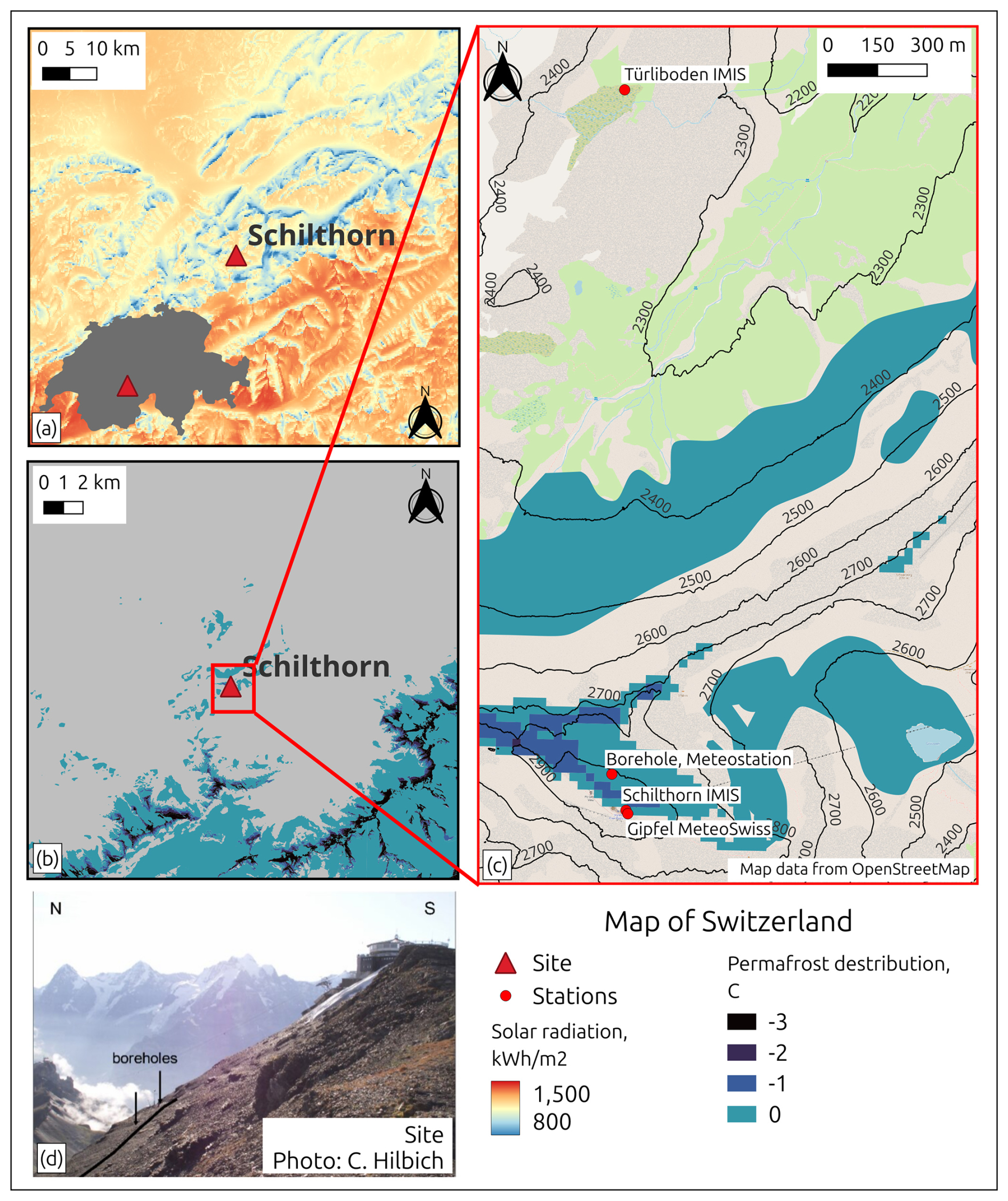
Figure 1 (a) Average yearly totals of solar radiation (Solargis, 2020) showing the Schilthorn site on an area map and on a map of Switzerland (grey shaded © swisstopo, 2024), (b) permafrost distribution adapted from Kenner (2018), (c) zoom into panel (contour lines © swisstopo, 2024) (b) indicating the site of Schilthorn borehole and surrounding meteorological stations Table 1, and (d) picture of borehole site and Schilthorn summit (Hilbich, 2010). Coordinates are based on UTM Zone 32T (EPSG:32632) for Switzerland. Schilthorn, E: 419500, N: 5158000. © (OpenStreetMap contributors, 2023) for the map data. Distributed under the Open Data Commons Open Database License (ODbL) v1.0. © QGIS Development Team, 2023 for the visualization of the map. All rights reserved.

(Swiss Permafrost Monitoring Network (PERMOS), 2024)Hoelzle et al., 2022Swiss Permafrost Monitoring Network (PERMOS) and Hoelzle, 2021

Table 1 Meteorological and borehole data used for modelling. IMIS denotes Intercantonal Measurement and Information System.

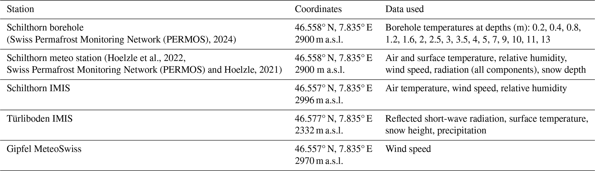
The borehole temperatures were obtained from the Schilthorn SCH_5198 borehole operated by PERMOS (Swiss Permafrost Monitoring Network (PERMOS), 2024). The borehole was established in 1998, it is 13 m deep and temperature is presently still measured. The ground temperature averaged over 13 m depth and over the period 1998 to 2025 was 0.02 °C (Swiss Permafrost Monitoring Network (PERMOS), 2024), the temperature range at the profile base is from −0.88 to 0.58 °C, and the ALT changes from 4.4 to 13 m. For simulations, we used atmospheric data (Table 1) from the PERMOS meteorological station next to the borehole for the years 2000 to 2017 (Swiss Permafrost Monitoring Network (PERMOS) and Hoelzle, 2021; Hoelzle et al., 2022). Long-term observations (Hoelzle et al., 2022) indicate that the mean air temperature observed at Schilthorn (1998–2018) is −2.60 °C, the mean snow height – 0.87 m, and the snow season usually lasts from October to June (Swiss Permafrost Monitoring Network (PERMOS) and Hoelzle, 2021). Due to the presence of gaps, the data were completed with data from the closest stations of the Intercantonal Measurement and Information System (IMIS) and MeteoSwiss network (Table 1) for the same time period. To reduce bias related to the input data used, correlations between the Schilthorn meteorological station and the other stations were calculated, and existing gaps were filled based on the regression coefficients obtained. The remaining gaps were filled using the MeteoIO data generation and interpolation functions (Bavay and Egger, 2014).

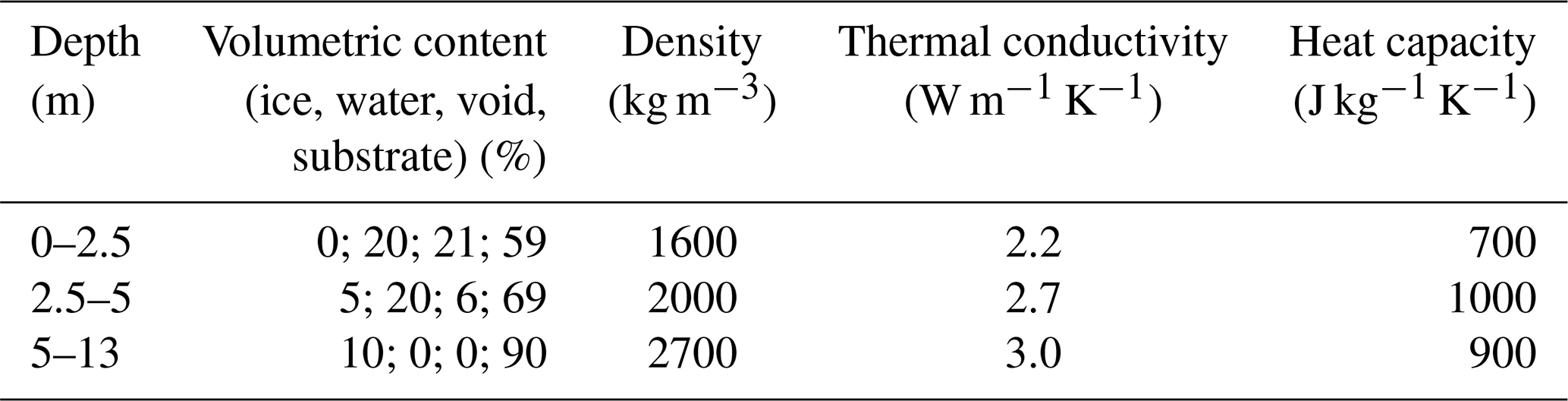
We set up the model using the following set of parameters: volumetric ice, water, substrate, and voids content of the ground, substrate density, thermal conductivity, and heat capacity. Based on the available data from the borehole temperature measurements and previous modelling experience (Marmy et al., 2013; Ekici et al., 2015; Wagner et al., 2019; Hoelzle et al., 2022), we use the substrate parameters listed in Table 2. The site is free of vegetation and the substrate consists of dark, deeply weathered limestone on the surface of mainly sandy and gravel debris of several metres in depth, lying over strongly jointed bedrock (Zappone and Kissling, 2021). The initial conditions required for the model were chosen to represent rocky ground, without specifying particular grain sizes for different layers. SNOWPACK requires appropriate initialization; however, a spin-up may not be necessary if the ground temperature profile is initialized using the corresponding observational data. Each layer was divided into grid cells with a vertical extent of 0.1 m. The upper layer consists of well-drained loose rock (talus) and thus has a lower water content and moderate porosity, which explains the lower heat capacity required to reproduce the temperature distribution. Below this, the heat capacity increases representing the presence of an active layer, which is indicated by long spring and autumn zero-curtains (Swiss Permafrost Monitoring Network (PERMOS), 2024). The zero-curtain effect occurs as a result of the latent heat release/consumption during the phase transition (thawing or freezing) in the active layer. At this time, the ground temperature remains close to 0 °C over an extended period, while the air temperature may vary significantly. At depth, the standard values for limestone are used. The values for density and thermal conductivity are determined according to the given substrate stratification. The geological map (Zappone and Kissling, 2021) indicates that the site has a limestone bedrock at depth, with sandy and gravel debris in the upper layers. This justifies the use of the recommended corresponding values for this type of ground (Table 2).

Table 2 Parameters of geological substrate for the Schilthorn site simulations.

4 Model simulations

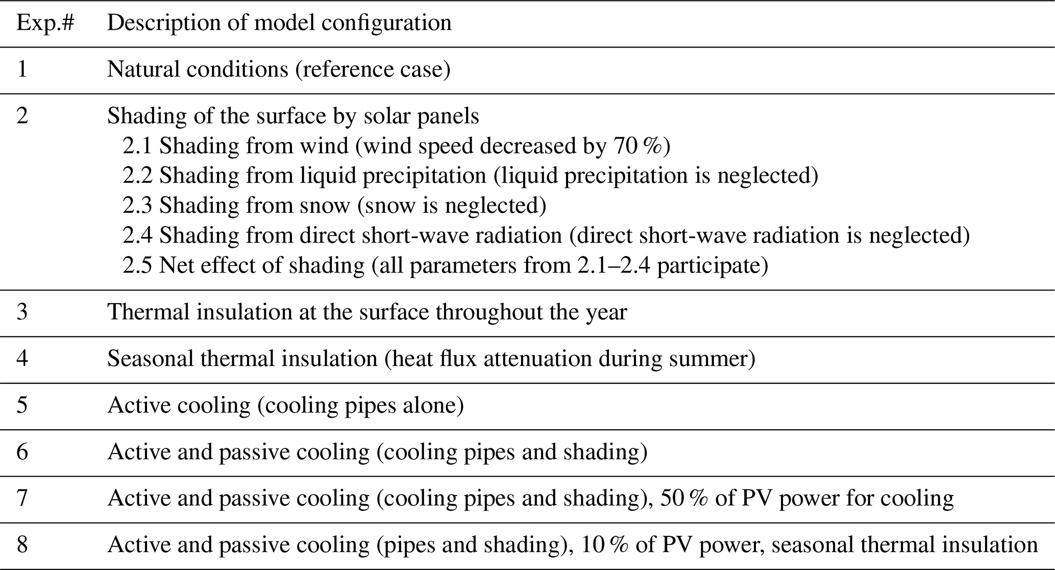
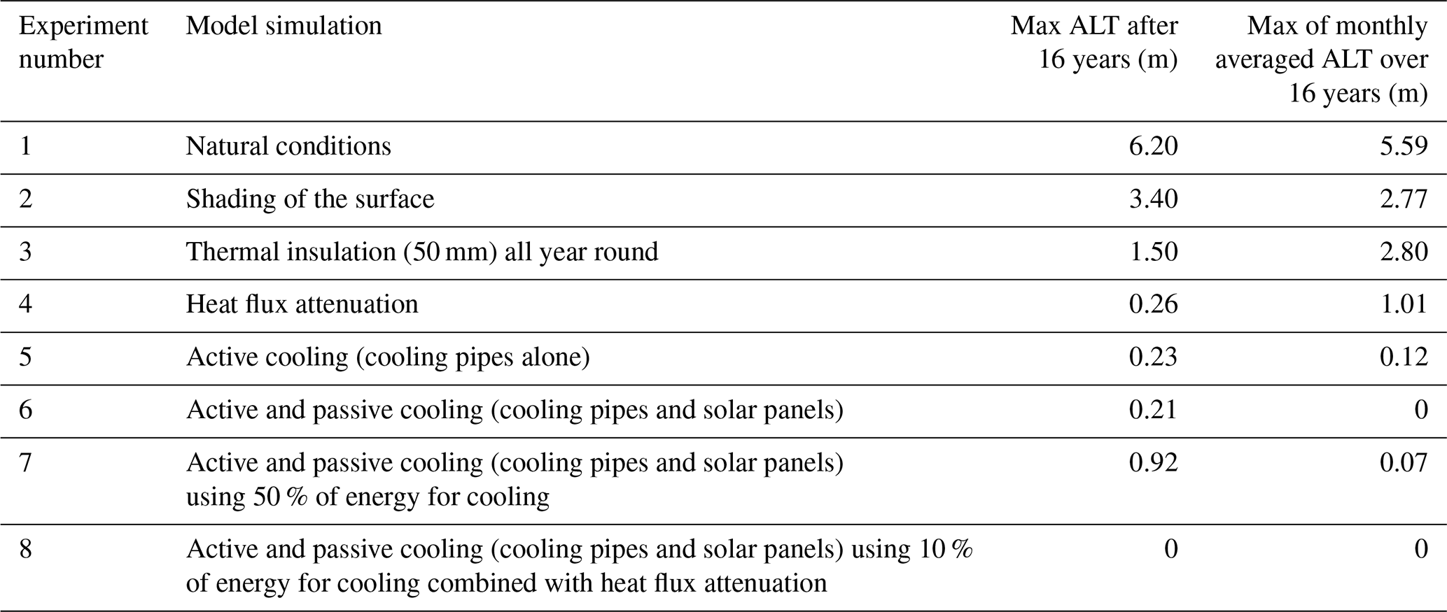
To understand the processes that occur in permafrost soils, different configurations of numerical simulations were employed, first simulating natural conditions without modifications and then applying different thermal stabilization methods. These simulations are numbered for easy reference and summarized in Table 3. The simulations were run for the period June 2000 to January 2017. This time frame was selected as it precedes the significant observed increase in ALT, aligns with available meteorological data, and represents long-term observations of permafrost temperatures at the site. Focusing on the period before the major increase in ALT provides a baseline reference and highlights how early intervention could have prevented subsequent degradation, serving as a cautionary example for similar at-risk sites. Starting simulations in June avoids defining an initial snow cover and related uncertainties in its properties. The simulation of this period allows reconstructing the impact from thermal stabilization methods and analysing the re-establishment of new temperature equilibrium within the ground, while preserving permafrost and delaying an increase in ALT at the site. This also allows to extrapolate obtained results to other similar permafrost sites. The model runs at an hourly time interval using meteorological forcing at 2 m above ground. This is a temporal resolution necessary to represent fast-changing weather conditions and to simulate their impacts, for instance, on the energy balance and its various heat fluxes. For coherence, the model uses the same 1 h time step. Internally, the model interpolates the hourly forcing on a 15 min time step (accomplished by the MeteoIO library; Bavay and Egger, 2014) to avoid abrupt step changes and to obtain higher temporal resolution simulations.

Table 3 Overview of model simulations.

4.1 Natural conditions

Numerical simulations of natural conditions were carried out as a reference case (Exp. #1, Table 3) to evaluate the performance of the model compared to the measured temperatures from the borehole. These simulations, combined with the study of the modelled and measured substrate parameters at this site (Pellet et al., 2016; Scherler et al., 2010; Marmy et al., 2016), allowed the correct setting to optimize the agreement of the modelled temperature distribution and the measured temperature data from the borehole. The soil albedo was set to 0.15 and we used the snow parametrization of Schmucki et al. (2014), which estimates the albedo based on the time elapsed since the last snowfall, grain size, and liquid water content (Lehning et al., 2002). The roughness length was set to 0.05 m accounting for the rocky surface. We used the Holtslag and Bruin (1988) correction model for atmospheric stability, which shows good performance on snow surfaces (Schlögl et al., 2017). We forced the model with available snow depth measurements from the site, avoiding the calculation of snow depth from precipitation data (Table 1) which includes only rainfall. In this way, we implicitly take into account local snow drift, since its effect is integrated in the observed snow depth. We force the model with incoming short-wave radiation, while the other energy balance components are computed by the model based on available meteorological forcing data (air temperature, wind speed, relative humidity, snow depth, and liquid precipitation equivalent) as well as the temperature at the base of the model domain for a full energy balance assessment. At the surface, a Neumann boundary condition was thus applied. The observed surface temperature data (Table 1) are not used directly as input for the model simulations, but serve to compare the model output with the measurements as a consistency check. At the base of the model domain, a Dirichlet boundary condition was used, prescribing borehole temperature measurements ranging from −0.9 to −0.1 °C.

We quantitatively compared the model output with the borehole temperature measurements using standard statistical analysis such as bias, root-mean-square error and correlation (Pearson coefficient) at different depths for monthly mean averages and for the whole time series. In addition, we compared the mean values and standard deviations for different model set-ups with observations. The set-up that produced the best performance was chosen as a reference case (Exp. #1).

4.2 Thermal stabilization modelling experiments

4.2.1 Shading of the surface

Surface shading from structures above the ground protects the soil from direct solar radiation, snow, and liquid precipitation. It also affects the wind speed near the ground. We simulate the shading of solar panels placed above the ground, exceeding the height of the snow cover, as proposed by Loktionov et al. (2022). To quantify the impact of shading of various parameters individually and in combination, we conducted experiments in two stages. In the first stage, we investigated the effect of each of the following parameters independently of each other: (1) wind speed decreased by 70 %; (2) the ground completely protected from snow and liquid precipitation; (3) only the diffuse component of incident short-wave radiation, which is derived from the reference case SNOWPACK simulation under natural conditions. In a second step, all parameters were modified simultaneously, simulating the combined effect on heat transfer and vertical temperature distribution.

Snow accumulation works as natural insulation; therefore, in winter it prevents heat loss from the ground and limits natural cooling (Wang et al., 2019). Liquid precipitation has a negative impact as it increases the ALT which accelerates permafrost degradation (Zhu et al., 2017; Wang et al., 2021). Changes in wind speed can have a positive or negative impact on permafrost, affecting heat transfer, snow re-distribution, and moisture content, which in turn can slow or accelerate permafrost degradation (Zhao and Yang, 2022). Based on these known effects, we designed our simulations to test the effect of neglecting individual components: wind, solid, and liquid precipitation, and direct solar radiation to better understand their respective roles in permafrost thermal dynamics.

The choice of parameters (1) and (2) was based on previous modelling results investigating thermal stabilization (Loktionov et al., 2022). However, Loktionov et al. (2022) instead applied a solar radiation value that was decreased by 95 % from global horizontal irradiance. In the present study, we can revert to the modelled components of direct and diffuse solar radiation. Using only the diffuse solar radiation component is a simplified and idealized case, which allows us to reproduce the effect of the solar panels on ground temperature distribution, without applying an additional empirical coefficient. Removal of the direct solar radiation component accordingly reduced the radiative heat flux from the atmosphere (Liu and Jordan, 1960; Olson and Rupper, 2019; Li et al., 2020). In reality, solar panels may have a different effect on the solar radiation reaching the ground beneath them, depending on their spacing and inclination. The numerical tests with these assumptions allow us to model the impact of the solar panels placed above the ground; however, for more accurate analysis, in situ experiments are required. The test results show the impact of each change on thermal stabilization and efficiency over the seasons.

4.2.2 Thermal insulation

We also model the ground covered with thermal insulation material. We simulate the presence of a 50–100 mm thick polystyrene slab with a thermal conductivity of 0.033 W m⁻¹ K⁻¹, a density of 28 kg m⁻³, and a heat capacity of 1500 J kg⁻¹ K⁻¹ to reduce heat transfer from the atmosphere to the ground (Loktionov et al., 2022). The thickness range was chosen such that efficient heat control in the context of this study was possible. We also simulated a thinner slab, which was found to be insufficient to reduce heat transfer. The insulation material also increases the surface albedo. In the model, this was implemented as an additional layer (styrofoam) at the top of the soil to preserve low temperatures at depth. Similar to the ground layers (Sect. 3), the thermal insulation layer and layers between 0 and 0.2 m were divided into grid cells of 0.05 m for both 50 and 100 mm material thickness. The albedo of the insulation material was set at 0.7, representative of white styrofoam with a high-albedo reflective coating (Ramamurthy et al., 2015; Qiu et al., 2018; Chen et al., 2020) and similar to a snow cover. Two particular cases were investigated: (1) insulation present all year round and (2) insulation present from the beginning of June until the end of October (under snow-free conditions) and lifted from November until the end of May to allow the natural cooling process. In (1), the insulating material protects the ground from direct contact with snow and rain. However, both types of precipitation accumulate on top of the protection layer, which is considered in the simulation. The objective of (2) is to regulate the heat flux (Sharaborova and Loktionov, 2022) by shielding during summer and favouring natural cooling in winter. The advantage of (2) is the combination of the shading effect of the solar panels (Sect. 5.2.1) with the ground insulation material. This approach has been introduced in the description of the method (Sharaborova and Loktionov, 2022) and is related to the attenuation of the conductive heat flux and temperature. In this configuration, heat flux attenuation and prevention of permafrost thawing are achieved without an external power supply. The method stabilizes frozen ground by insulating the soil in warm seasons by protecting the ground from solar radiation and precipitation, and by limiting convective heat transfer. Elevating the insulation above snow cover in winter helps to use natural air circulation for cooling.

4.2.3 Thermal stabilization with active cooling

This experiment (Exp. #5, Table 3) simulates the case of thermal stabilization using a solar-powered heat pump (Sharaborova et al., 2022a). The system combines the previously described passive protection (Sect. 4.2.1), where solar panels act as sunscreens and as a power source for the heat pump cooling the ground through cooling pipes. The latter are modelled by implementing a sink term at the level of the pipes that corresponds to the energy supplied by the solar panels keeping the ground temperatures around the pipes below 0 °C.

Similar to previous studies simulating the application of a thermal stabilization system (Loktionov et al., 2022), we model cooling pipes applying a negative advective heat (q_adv) in the layers concerned. The advective heat is implemented in the following way: first, the energy obtained from the solar panel is calculated using incoming short-wave radiation (ISWR), the solar panel surface area (A = 1 m²), and the PV conversion efficiency (η = 10 %), as detailed in Eq. (1). Then, this power is applied to cooling, using the cooling energy efficiency rate (EER), Eq. (2), which is related to the coefficient of performance (COP) for cooling machines and for heat pumps, according to Eq. (3), and depends on the ambient (atmospheric) temperature. Equation (2) is adapted from Loktionov et al. (2022), the coefficients are specific to the equipment used. Finally, to determine the advective heat applied in the model, the cooling capacity is divided by the volume of the layer that contains the cooling pipes. This procedure is described using the following equations:

$$\begin{array}{}\text{(1)}& {\displaystyle }{q}_{\mathrm{adv}.\mathrm{heat}}={\displaystyle \frac{\text{ISWR}\cdot \mathit{\eta }\cdot A\cdot \text{EER}}{V}},\text{(2)}& {\displaystyle }\text{EER}=\mathrm{4.8}-\mathrm{0.12}\cdot T_{\mathrm{a}},\text{(3)}& {\displaystyle }\text{EER}=\text{COP}-\mathrm{1}.\end{array}$$

Advective cooling was applied for the months of April to October. The cooling pipes are integrated into the model in a layer from 20 to 22.5 cm (the diameter of the pipe is 25 mm), cooling this layer to a minimum temperature of −7.5 °C, which corresponds to the mean temperature of the coolant circulating in the pipes (Loktionov et al., 2024a). To accurately represent this process, the grid cell thickness for layers between 0 and 0.8 m was refined to 0.005 m. Active cooling from pipes creates a thermal barrier layer of a cold (frozen) slab inside the ground that protects the permafrost in summer from heat conducted from the surface deeper into the ground. Exp. #5 (Table 3) applies active cooling alone without shading the soil with solar panels. Exp. #6 (Table 3) combines passive and active cooling. In both experiments, the cooled area corresponds exactly to the area of the solar panels. However, in real life, this relation will be more complex, depending on the time of day, local topography, ground parameters, etc. Later in this study, we also examine cases in which only a portion of the energy from solar panels is reserved for cooling (Sect. 5.3).

5 Results and discussion

5.1 Natural conditions

The simulated evolution of ground temperature and observed snow depth at the Schilthorn site is shown in Fig. 2 for the observation period from 2000 to 2017. By studying Schilthorn during a period when the ALT was thinner and before significant changes occurred, we gain valuable insights into the dynamics of mountain permafrost. The seasonal ALT is indicated by the 0 °C isotherm and the temperature at the base of the model domain corresponds to the measured permafrost temperature in the borehole. We also observed an increase in ALT over the years from approximately 5 m to almost 7 m. In natural conditions, a realistic computation of the ground heat flux depends on an accurate representation of the snow depth as shown in Fig. A1, where the modelled and measured snow align closely for most winters. For some periods, the measured snow depth is below the simulated values, indicating that the model underestimates compaction, melt, and erosion (Lehning et al., 1999). Figure 3a indicates that the modelled temperatures are slightly higher than measured. However, the monthly average difference for the entire simulation period never exceeds 1 °C. Figure 3b indicates that the model and the observations are comparable with similar long-term mean temperatures and standard deviations throughout the vertical profile, evidenced by correlation coefficients greater than 0.8, except for the middle layers, especially at depth around 5 m, where the coefficient drops to almost 0.6. This depth corresponds to the ALT, where even small temperature variations (on the order of a tenth of a degree) can cause significant fluctuations in its position (Marmy et al., 2016).

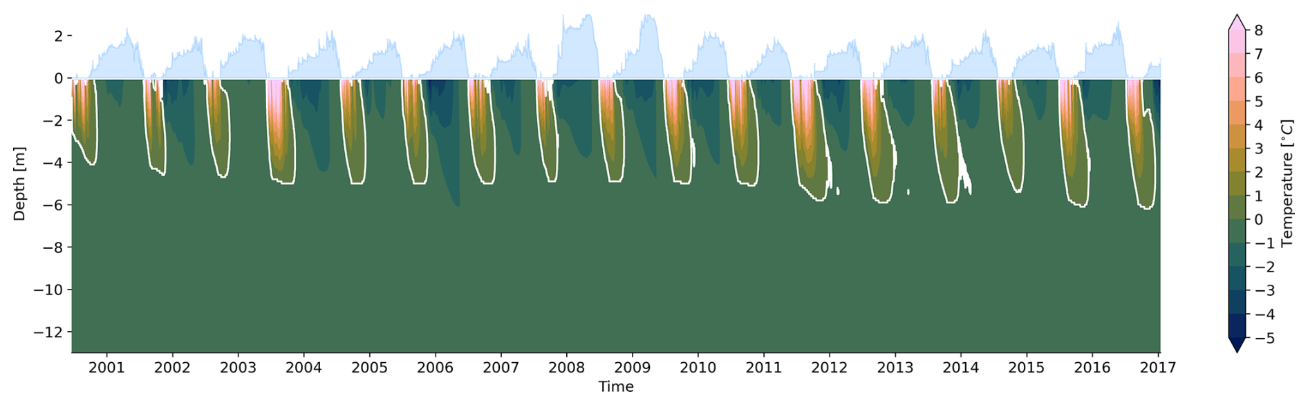
Figure 2 Time series of daily averaged modelled ground temperatures during natural undisturbed conditions at the Schilthorn site from 2000 to 2017. White contours indicate the 0 °C isotherm, i.e, the ALT. Snow depth is indicated in light blue above the 0 m depth level.

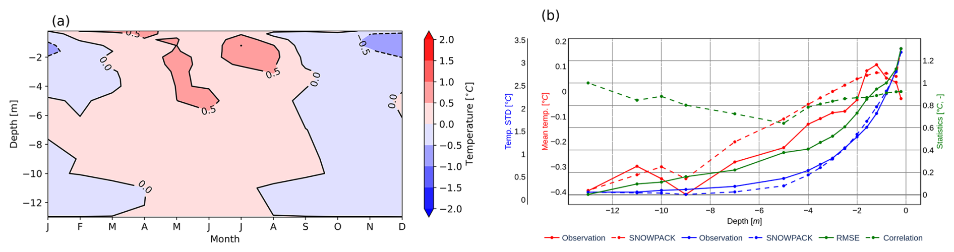
Figure 3 Comparison between modelled and measured ground temperatures at the Schilthorn site from 2000 to 2017. (a) Monthly averaged differences. Red (blue) colours indicate model temperature higher (lower) than observations. (b) Statistical analysis of the ground temperature differences averaged over the 17 years period. The 3 vertical axes represent: mean temperature (red), standard deviation (blue), other statistics (green). The horizontal axis indicates depth.

5.2 Thermal stabilization experiments

5.2.1 Shading of the surface

We studied the impact of shading on the ground temperature in several experiments, isolating the effect of individual elements as described in Sect. 4.2.1 and comparing the simulations with the averaged natural conditions (Fig. A2) as described above. Reduction of liquid precipitation by sheltering effects results in the smallest temperature changes in the ground (Fig. 4d). The absence of liquid precipitation results in better cooling in winter and leads to a reduction in ALT thickness. Lower wind speed results in more efficient cooling for the full year (Fig. 4a, b) as a result of changes in sensible heat fluxes on the surface. The greatest effect is seen when the natural isolating snow cover is absent (Fig. 4e, f). This change results in a notable cooling of the ground in winter that supports the preservation of permafrost (Fig. 4e). However, temperatures in summer increase because snow cover does not protect the ground from heat exposure and the favourable albedo effect is missing. If no snow is accumulated, the benefit of natural insulation is lost and the warming of the ground starts earlier than otherwise (Fig. 4f). Heat loss during winter is not enough to compensate for the absence of snow. Finally, shading the ground from direct short-wave radiation (Fig. 4g, h) results in lower ground temperatures in winter and, especially, in the summer season. This occurs because the incident radiative energy does not reach the ground and, as a result, the ALT (0 °C) is smaller.

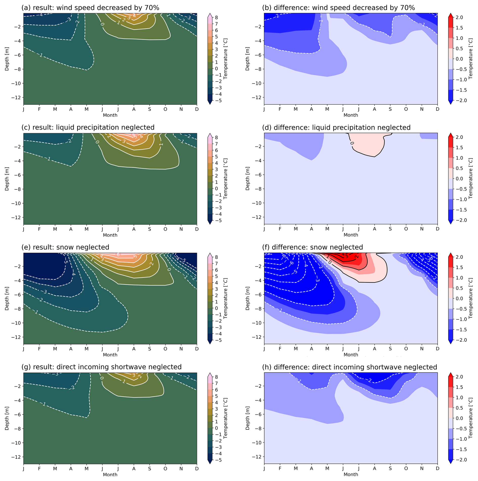
Figure 4 Monthly averaged modelled ground temperatures at the Schilthorn site from 2000 to 2017 resulting from individual model configurations defined in the shading experiment (Exp. #2, Table 3). (a, c, e, g) Simulated ground temperature, (b, d, f, h) difference between simulated and natural conditions. Red (blue) colours indicate model temperature higher (lower) than observations. Experiments shown: (a, b) wind speed reduced by 70 % (Exp. #2.1); (c, d) liquid precipitation set equal to zero (Exp. #2.2); (e, f) snow depth set equal to zero (Exp. #2.3); (g, h) direct component of incoming short-wave radiation neglected (Exp. #2.4).

In Fig. 5 the net effect of shading at Schilthorn is shown, demonstrating that shading leads to cooling of the ground during winter and a decrease in ALT (depicted as the 0 °C isotherm in both figures). In agreement with the results by Quinton et al. (2011) testing different shading devices and observing the ground temperature decreasing with time, we also find a decreasing trend in ground temperature in our simulation results. However, there is still enough heat input to keep the ALT at a depth of several metres (Table D1). This indicates that this stabilization method is insufficient and needs to be supplemented by other elements described by Cheng (2005) and Loktionov et al. (2022). In contrast, the method amplifies the annual cycle of thawing and refreezing. In the long-term trend (Fig. 5), the net effect of this method allows rapid ground cooling every winter; however, it does not create and maintain a thermal barrier layer even after 16 years.

Figure 5 Time series of daily averaged modelled ground temperatures presenting the net effect of the shading experiment (Exp. #2.5, Table 3) at the Schilthorn site for the period of 2000 to 2017. White contours indicate the 0 °C isotherm, i.e. the ALT.

5.2.2 Thermal insulation

In Fig. 6, the effect of an artificial thermal insulation layer throughout the year is shown, presenting the monthly average evolution of the ground temperature profile of the Schilthorn borehole. We examine two cases with different thicknesses of the thermal insulation layer of 50 and 100 mm. Although the placement of an insulation layer of 50 mm does not completely prevent temperatures above 0 °C (Fig. 6a) it decreases the ALT in summer. In addition, Figs. 6b and B1 demonstrate that the placement of an artificial insulation layer (Exp. #3, Table 3) effectively decreases the loss of heat to the atmosphere in winter. The distribution of heat flux in the permafrost remains preserved, due to the limitation in heat flux at the surface (Fig. B1). However, in the long term, the combination of atmospheric and geothermal heat fluxes will warm the permafrost. Consequently, installation of an insulation layer of 50 mm thickness at the surface is insufficient to preserve the permafrost table, and the ALT still comprises several metres (Fig. 6a, Table D1).

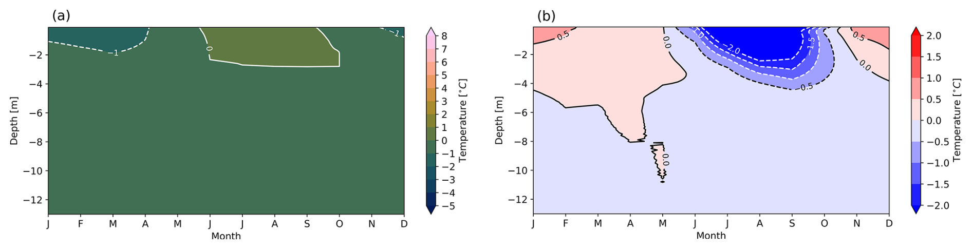
Figure 6 Modelled monthly averaged ground temperatures at the Schilthorn site for the period from 2000 to 2017 using a 50 mm artificial thermal insulation layer on top of the ground throughout the year (Exp. #3, Table 3). (a) Temperature evolution in the ground. (b) Temperature difference compared to the undisturbed natural conditions. Red (blue) colours indicate model temperature higher (lower) than measurements.

The results presented in Fig. B2 show that the thicker the thermal insulation layer, the smaller its effect of thermal stabilization. Instead of favouring ground cooling during winter, this artificial thermal insulation prevents the desired heat loss from the ground to the atmosphere. In addition, it can be seen that decreasing the thickness of the insulation layer allows some cooling in winter, but at the same time protects the ground less from heating in summer. The observed effects are plausible because snow accumulates above the thermal insulation layer in winter, reducing the loss of heat from the ground. This suggests the existence of an optimal thermal insulation thickness. However, this optimum naturally depends on latitude, altitude, exposition, slope angle, local topography, and climatic conditions. Given the principal interest in quantitatively assessing different engineering-based permafrost thermal stabilization methods, we did not strive to determine this optimum for the Schilthorn site and consider it outside of the scope of this study. The brief conclusion here is that the 50 mm thickness yielded a better effect during summer and winter, compared to cases with increased (100 mm) and decreased (10 mm) layer thickness. However, it also appears that this method is not efficient enough to protect local alpine permafrost in the long term from the growing impact of atmospheric warming and increasing net energy input into the ground.

The timely placement/lifting of the insulation layer is the key to most effective cooling during winter and better preservation during summer. We examined the effect of heat transfer control by combining the impact of thermal insulation with surface shading. Figure 7 shows that this approach (Exp. #4, Table 3) results in intense winter cooling over a multi-year period while favouring heat loss from the ground to a depth of about 10 m (Fig. 7a). In this case, heat flux attenuation (Sharaborova and Loktionov, 2022) is sufficient for thermal stabilization of the permafrost (Table D1) and is more efficient in cooling when installed on site than continuous thermal insulation (Luo et al., 2018). This method also results in a gradual decrease in ALT over the years, demonstrating that the winter cooling effect surpasses the summer warming. In addition, thermal insulation during the summer helps to protect the permafrost by reducing the transfer of heat from the atmosphere. Taking a closer look at the last year of the simulation (Fig. 7b) reveals a temperature decrease in near-surface layers and a significant reduction in ALT with this approach. Figure B3 indicates the continuous loss of heat during winter, which explains the preservation of low ground temperatures. This cooling mechanism can be sufficient for creating a thermal (cold) barrier layer near the surface to protect the ground underneath over a whole year (Fig. 7). Although the creation of a barrier layer takes several years in the simulation, with unstable conditions occurring during its formation, after 16 years the ALT was decreased to several decimetres. We expect this method to be even more effective when used in combination with active cooling since it creates an additional “shield” of thermal insulation and further decreases heat exchange with the atmosphere.

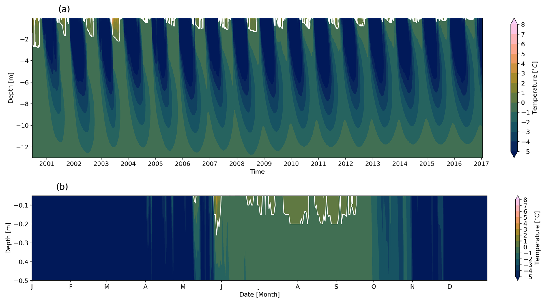
Figure 7 (a) Time series of daily averaged modelled ground temperatures from the heat transfer attenuation experiment, (Exp. #4, Table 3) at the Schilthorn site for the period of 2000 to 2017. White contours indicate the 0 °C isotherm, i.e. the ALT. (b) Last year of the simulation, 2016, after 16 years of artificial thermal insulation of the ground.

5.2.3 Thermal stabilization with active cooling

We now examine the effect of the proposed thermal stabilization system with active cooling (Sect. 4.2.3), first quantifying the effect of the cooling pipes alone (Exp. #5, Table 3) and then the combined effect of the system that includes shading of the ground from the solar panels (Exp. #6, Table 3). We examine the distribution of temperature and heat flux in the ground to observe whether a thermal barrier layer is developing.

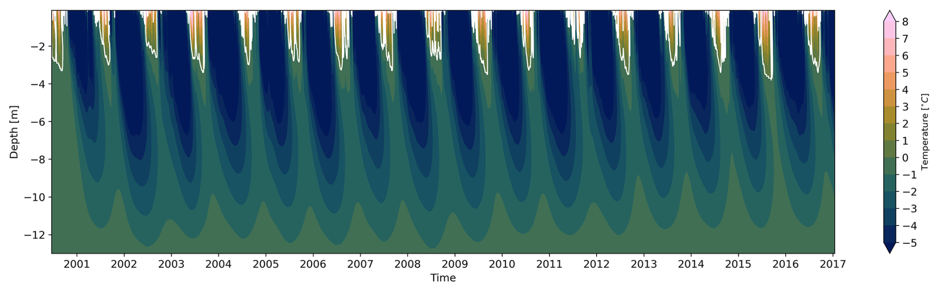
Figure 8 shows that when active cooling is applied (Exp. #5, Table 3), sub-zero temperatures of the permafrost establish after 4 years with temperatures well below 0 °C at depth. The upper layers of the last simulated year (Fig. 8b) show that the thawing boundary, indicated by the 0 °C contour, does not extend deeper than 25 cm demonstrating the effectiveness of the cooling method in creating a thermal barrier layer and limiting heat transfer during summer.

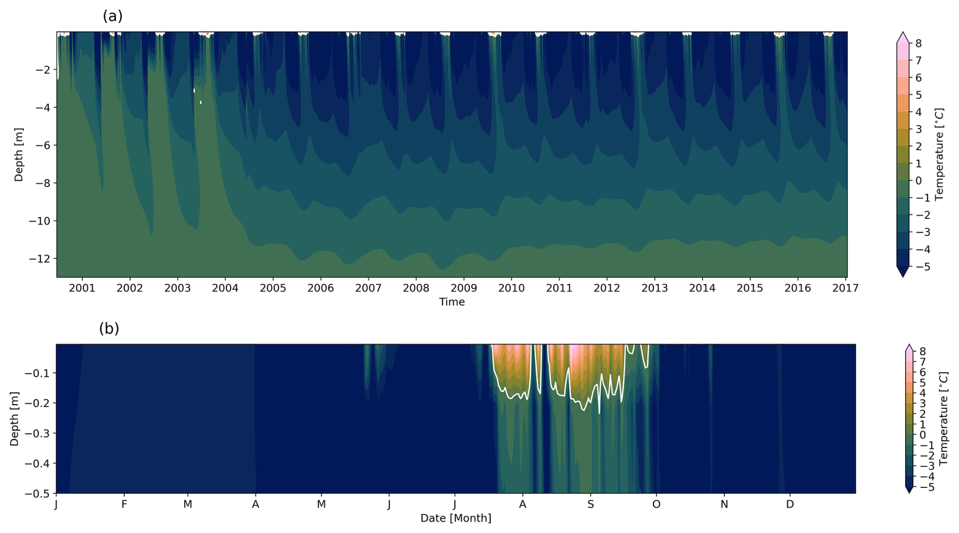
Figure 8 (a) Time series of daily averaged modelled ground temperatures from the cooling pipes experiment (Exp. #5, Table 3) at the Schilthorn site for the period of 2000 to 2017. White contours indicate the 0 °C isotherm, i.e. the ALT. (b) Last year of the simulation, 2016, after 16 years of active cooling.

The distribution of heat flux shown in Fig. 9 (Exp. #5, Table 3) illustrates the consequences of the formation of a thermal barrier layer. The large heat fluxes in the upper layers are due to the strong temperature gradient between the ground surface and the cooling pipes, the latter conserving a constant low temperature around them. This determines the direction of the heat flux downward from the surface to the level of the pipes. In depth, the heat flux is directed upward toward the pipes. Together, these heat fluxes indicate the extraction of heat from the ground through the cooling liquid that circulates in the pipes.

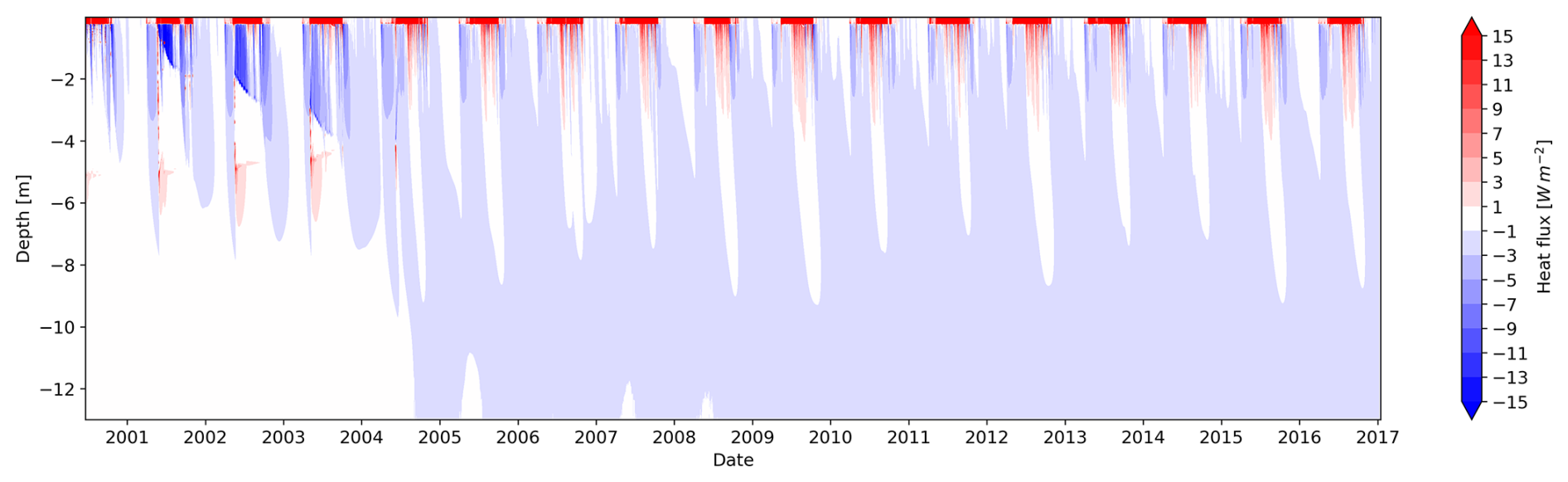
Figure 9 Time series of daily averaged modelled conductive heat flux from the cooling pipes experiment (Exp. #5, Table 3) at the Schilthorn site for the period of 2000 to 2017.

Figure 8a shows that after the establishment of the barrier layer (after approx. 4 years), the soil cools to a level of approximately 3 m, which may be related to the structural stratigraphy of the ground given (Table 2). Due to thermal inertia and slow heat conduction in the ground, it takes several years to form a stable thermal barrier layer (Fig. 8). Once enough heat is lost from the ground, the system switches from cooling to keeping the in-depth temperatures stable in the following years. Due to the temperature boundary conditions at the bottom of the model domain (Sect. 4.1) the model evolves toward a steady state (Fig. 9).

We now focus on the full system that combines active and passive cooling methods, i.e. including shading with the solar panels (Exp. #6, Table 3). The simulation results presented in Fig. 10 show that this combined effect is favourable for the preservation of permafrost due to the formation of a more pronounced sub-freezing thermal barrier layer compared to the results of both systems independently. The effect is also more immediate and does not take several years to establish the thermal barrier layer (Fig. 10a). In the last year of the simulation (Fig. 10b), it is evident that the impact of summer warming cannot be fully suppressed or compensated for. However, the engineered cooling method significantly reduces the ALT compared to natural conditions, achieving a difference of several metres. Our results show that the combination of active and passive cooling is sufficient to stabilize not only the continuous permafrost of the lowlands, as shown by Loktionov et al. (2022), but also the mountain permafrost (Table D1).

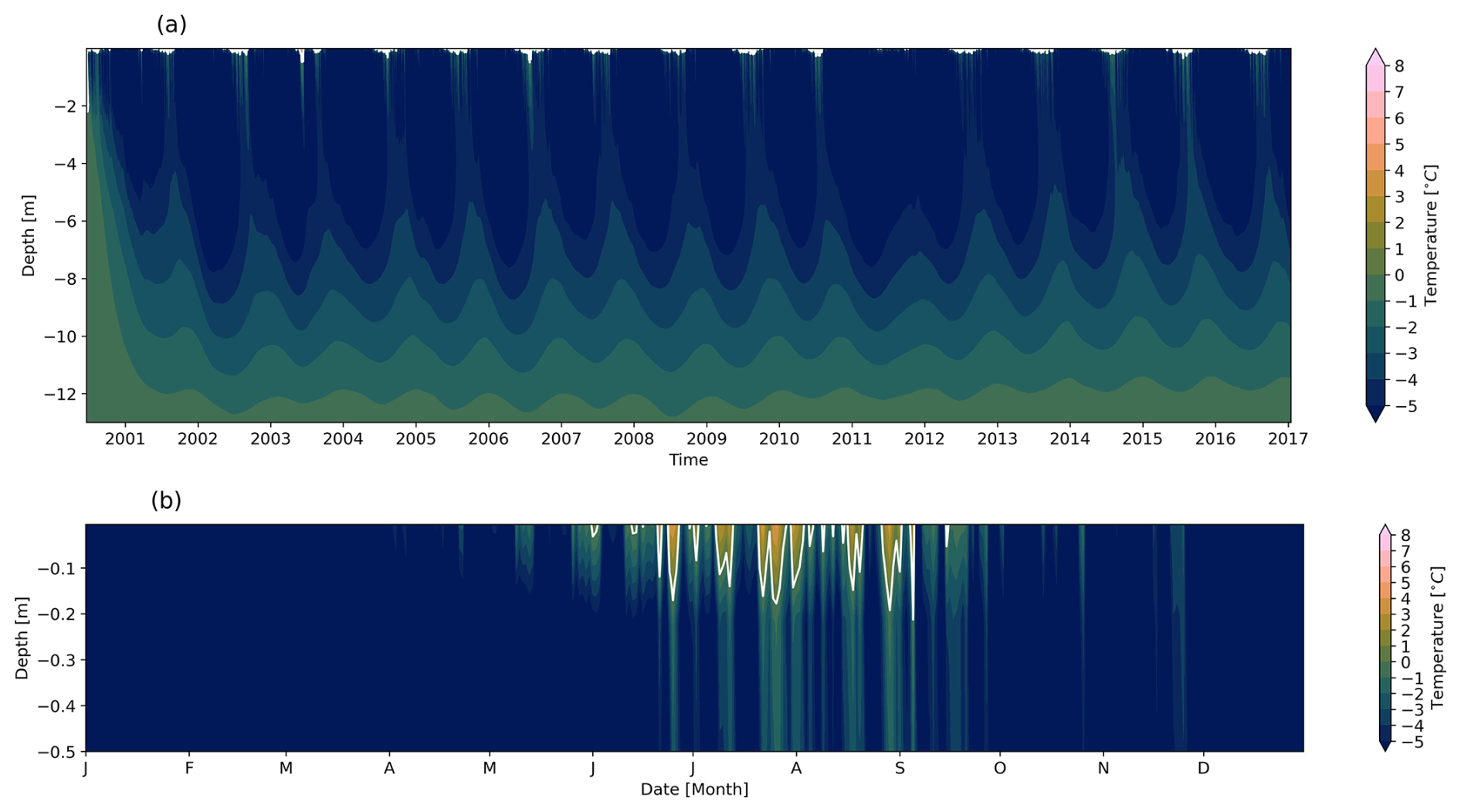
Figure 10 (a) Time series of daily averaged modelled ground temperatures from the experiment combining cooling pipes and solar panel shading (Exp. #6, Table 3) at the Schilthorn site for the period of 2000 to 2017. White contours indicate the 0 °C isotherm, i.e. the ALT. (b) Last year of the simulation, 2016, after 16 years of active cooling and shading.

The evolution of the conductive heat flux initiated by the combined cooling system (Exp. #6, Table 3) (Fig. 11) shows that in addition to the effect of the cooling pipes, passive cooling works during the winter season. This corresponds to heat evacuation from depth in winter, when the heat flux direction is upwards (Fig. 11a). Figure 11b indicates that the highest heat flux values occur in the layer between the surface and the pipes from April to the end of October, when active cooling is applied. This downward heat flux extends to the cooling pipes, which arises as a result of the strongest temperature gradient. Below this level, the heat flux eventually decreases to 0 W m⁻². In winter, heat is lost to the cold atmosphere, reversing the direction of heat conduction. Figure C1 presents the daily heat flux and temperature profiles, illustrating the evolution of conductive heat flux and ground temperatures over time and highlighting their dynamic behaviour throughout the simulation.

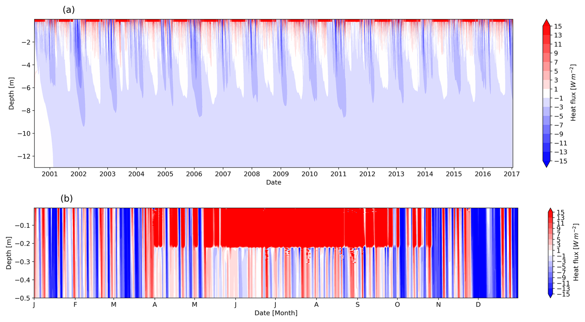
Figure 11 (a) Time series of daily averaged modelled conductive heat flux from the experiment combining cooling pipes and solar panel shading (Exp. #6, Table 3) at the Schilthorn site for the period of 2000 to 2017. (b) Last year of the simulation, 2016, after 16 years of active cooling and shading.

5.3 Analysis and discussion of stabilization effects

For the mountain regions considered, the most efficient method of thermal stabilization was active cooling combined with effects from passive methods such as surface shading with solar panels. In the experiments described so far (Sect. 5.2.3) all the PV energy produced was used to power the heat pump. The main objective is to set as much energy as needed for cooling. However, we also tested the case where only a partial amount of the available PV energy is reserved for cooling. This case may serve as a more realistic and practical demonstration of the system application, as it could imply the potential to use smaller panels or other optimizations in system design. It allows for challenging the system, in case the surface for installation is limited and the energy should be redistributed between cooling and other infrastructure energy supply. We show a situation in which only 50 % of the incident solar radiation is used to power the heat pump, i.e. for cooling (Exp. #7, Table 3), reserving the other half for the power grid or other needs in the vicinity of the site. Recall that the cooled surface has the same area as that of the solar panels (Sect. 4.2.3). In the following part, we perform some experimental tests, cutting the energy supply directed to cooling by a certain amount, to look at the resilience of the system in different configurations.

In the case where only half of the generated PV energy is used for cooling (Exp. #7, Fig. 12), we applied cooling in summer, similar to the case discussed in Sect. 5.2.3 Exp. #6, where cooling occurs from April to October. This energy partition between cooling and the grid aims to maintain the same temperature and persistence of the barrier layer as in Exp. #6 (Fig. 10). However, with half the amount of cooling power, the barrier layer is not as stable as with the 100 % energy supply. In addition, the ALT increases when using less power (Fig. 12b) compared to the case applying 100 % (Fig. 10b). Recall that the creation of an efficient barrier layer only with cooling pipes requires five full seasons with 100 % power supply, applying cooling from April to October. It can be seen that, due to the initial adjustment process creating the thermal barrier layer, most of the PV energy is initially used to cool the system. Once the barrier layer is established and stable in time, a larger fraction of the produced PV energy can be injected into the grid. However, we note that active cooling may not necessarily need to bring the system to a new equilibrium, and maintaining the existing thermal balance might be sufficient. It should further be noted that our results did not explicitly test this; we assumed a simplified case in which the energy is evenly split between cooling and grid injection. In a real-world application, the system control will become completely dynamic, an ultimate goal of the system application. Priority should be given to cooling before feeding into the grid. For the design of a suitable PV system, it is therefore imperative to know the energy demand for the creation and maintenance of a thermal barrier layer in alpine permafrost, which can be obtained from numerical simulations, as demonstrated in the previous sections. The optimal choice will enable reliable cooling of the ground while bearing the potential of providing significant excess power to the grid or nearby installation, especially after the initial ramp-up time.

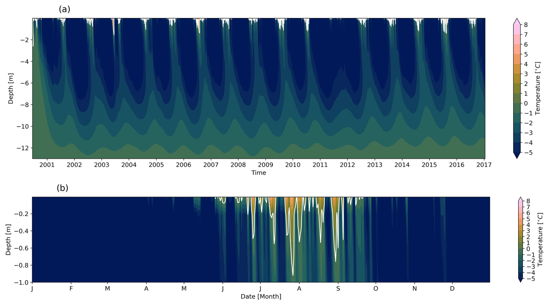
Figure 12 (a) Time series of daily averaged modelled ground temperatures from the experiment combining cooling pipes and solar panel shading but using only 50 % of available energy for cooling (Exp. #7, Table 3) at the Schilthorn site for the period of 2000 to 2017. White contours indicate the 0 °C isotherm, i.e. the ALT. (b) Last year of the simulation, 2016, after 16 years of active cooling and shading.

Another alternative is the combination of active cooling (Exp. #6, Table 3) with heat flux attenuation (Exp. #4, Table 3) as discussed in Sect. 5.2.2 and presented in Fig. 7, when during summer the ground was also protected with thermal insulation material. In that case, it is not necessary to wait until the snow has melted to lay out the thermal insulation as discussed in Sect. 5.2.2; however, it is important that the application of thermal insulation to attenuate heat flux is coordinated with the period of active cooling. During the active cooling period (April to October), thermal insulation is placed on the ground and removed when it is deactivated to allow effective winter cooling. This set-up improves the efficiency of the cooling system by preserving low ground temperatures in summer while allowing natural cooling in winter. In this case, a 50 mm thick thermal insulation is simulated and was found to be efficient protection. The combination of active cooling, shading, and heat flux attenuation leads to the desired stabilization effect. It allows us to use less PV energy for cooling and send more to the grid even in the case where the cooled surface area is equivalent to the surface of the solar panels used. As in experiments #7–#8, we tested different cases when only a certain amount of the available PV power is used for cooling. Here, due to the effective preservation of cold in the ground established by heat flux attenuation, we found for our test site that when combining active cooling with heat flux attenuation the energy required for cooling can be as low as 10 % of the produced PV power (Exp. #8, Table 3).

As visible in Fig. 13, the conservation of the cold temperature resulting from thermal insulation helps to keep the ALT shallow. This results in more efficient cooling and heat loss from the ground compared to cases of active cooling alone (Fig. 8), or active cooling with shading (Fig. 10). Another positive aspect of this combined method is that not all the PV power produced is used for cooling only, as was the case in Exp. #6 (Fig. 10). Limiting the energy used for cooling without modifying the natural conductive heat flux is possible but recommended to be 50 % or higher; otherwise, the active layer will remain deep. When combined with heat flux attenuation, this approach offers greater flexibility in managing the power received from solar panels. We also suggest that intense and continuous cooling might be unnecessary; it can be adjusted based on the monitored state of the permafrost, its temperatures, and also on atmospheric conditions. The latter determine which combinations of the stabilization systems should be applied in different climatic conditions. Although site-specific decisions require local calibration, our simulations provide a basis for such adaptive strategies. The simulated ALT results are listed in Table D1 for a better overview and comparison.

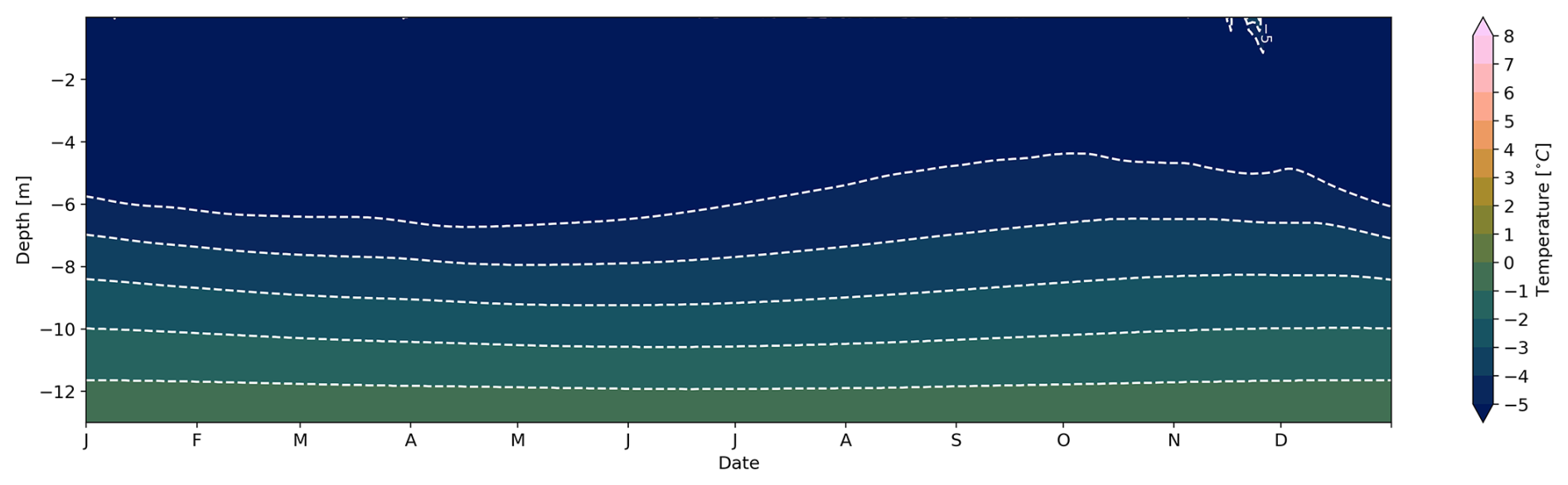
Figure 13 Daily averaged modelled temperature from the experiment combining heat flux attenuation by thermal insulation with active cooling and shading using only 10 % of the produced PV power for cooling (Exp. #8, Table 3) at the Schilthorn showing the last year of the simulation, 2016, after 16 years of active and passive cooling.

Knowing the amount of energy required for cooling, creating and maintaining an effective thermal barrier layer to stabilize the underlying permafrost allows optimal system design and power regulation. Simulations have shown that only a fraction of the produced PV energy (50 % for active cooling alone and 10 % for active cooling combined with heat flux attenuation) is necessary for direct cooling of the ground. The excess energy is then available for the grid. In an advanced application, the stabilization system could be dynamically regulated depending on the monitored state of the permafrost. However, optimal performance of the combination of active and passive cooling is difficult to achieve in the field due to local climate effects and complicated installation in complex alpine permafrost terrain. In such cases, the use of a system similar to Loktionov et al. (2024b) could be an alternative, cooling parts of constructions directly with cooling pipes attached to basement walls, taking advantage of unused space in the foundation of a building, and avoiding the installation of cooling pipes on inaccessible surfaces such as bedrock.

Despite the efficiency of the cooling system and its ability to create a thermal barrier layer, additional aspects must be taken into account, for instance, the topography of the terrain, water in the ground and associated heave, and difficulties linked with building in mountain permafrost that may cause some risks to infrastructure and the cooling system itself. One of the dangers is moisture present in the substrate during active cooling (Sect. 5.2.3) which can lead to heave and potential destruction of cooling pipes and solar panels, and cause damage to nearby structures. That is why for specific applications the simulated case must be adapted according to local ground properties and moisture conditions, the existing ground temperature distribution, ground-atmosphere heat exchange, topography, exposition, local climate, and potentially existing construction characteristics. It remains a challenge to apply a thermal stabilization system in alpine permafrost without altering the structure and mechanical processes in the ground.

Up-scaling the system to larger cooling areas is another direction of research. The presented numerical modelling framework could be extended to other permafrost types, e.g. continuous (Arctic and Polar regions) and discontinuous (Subarctic regions), to investigate the performance of thermal stabilization systems in different climatic regions and to propose an optimal combination of system components for these conditions. The present study constitutes a detailed and systematic numerical investigation of the choice and performance of permafrost stabilization methods. The results are intended for the design and implementation of prototype installations and for up-scaling to real-world applications. The forthcoming challenges involve conducting experimental tests to validate the hypothesis, evaluating the influence of climate change on permafrost dynamics both with and without stabilization measures, and devising an optimized methodology for thermal stabilization tailored to diverse sites and climate conditions.

5.4 Model assumptions and limitations

In the following, we consider the limitations of the modelling framework and the implications of key assumptions that may influence the findings.

Due to the nature of simplified and idealized 1D simulations, that is, solar panels completely protect the ground without gaps between adjacent panels from snow and precipitation, no lateral snow drift, and the applied coefficient for wind speed decrease is empirical and its realistic value requires more advanced estimation (Sect. 5.2.1 and 5.2). In addition, the use of 1D simulations limits the investigation of 3D effects such as subsurface lateral heat flow and complex geometric configurations of infrastructure. This simplification may not fully capture interactions present in real-world applications, particularly when optimizing cooling pipe layouts under heterogeneous geo-cryologic conditions.

Another limitation of the 1D formulation is the representation of the pipe cooling system. The model prescribes a constant temperature in the pipe, not considering the fluid temperature difference at the entrance and exit of the pipe due to heat exchange with the surrounding ground, as would be the case in a 3D situation. Another approximation is that the calculation of the power required for cooling is simplified and is effective only in the presence of solar radiation. The current state of the model allows us to assess the thermal stabilization potential of a system and show its effects when applied at a permafrost site. However, for a real-world application, a full 3D model and a real-time monitoring system should be used to dynamically adapt the necessary cooling power supply according to the conditions of the permafrost and the solar power production. In addition, further refinement of the system is needed for an optimal choice of system variables such as the depth and spacing of the cooling pipes, the thickness of a thermal insulation layer, and the most efficient and economic way to create and maintain a thermal barrier layer while regulating power to dynamically adapt to real-time permafrost conditions and ALT. The geometric configuration of the cooling pipes in the ground needs to be adjusted to the local geo-cryologic, topographic, and climatic conditions for sufficient and most efficient ground cooling.

The simulation framework employs a bucket water scheme, which has inherent limitations in representing soil water retention and redistribution. Although more detailed approaches such as the Richards equation could capture capillary-driven and preferential flow, these rely on assumptions that may not hold in coarse, rocky permafrost soils where voids and cracks dominate and capillary action is minimal. Therefore, it is uncertain whether the Richards equation would offer improved accuracy in such terrain. In addition, given the slope of the terrain at the site, percolating water may not only seep vertically but also laterally, which is not accounted for in the current model. More relevant is probably considering slope flow and water percolation in a 3D version of the model.

In addition, although SNOWPACK includes evaporation, its interaction with the bucket scheme simplifies the representation of latent heat exchange. In this model, only the surface layer contributes to evaporation, and once it dries out, evaporation ceases. This limits the model's ability to simulate continuous moisture-driven cooling via latent heat fluxes.

6 Conclusions

Thawing permafrost triggers hazards such as structural damage, rockfalls, and landslides, which increasingly threaten the stability of mountain infrastructure, while current mitigation methods struggle to adapt to rapid climate change. This study investigates the Schilthorn site in the Bernese Alps, Switzerland, where the ALT has doubled over the past decade, highlighting its vulnerability to climate change. Using the 1D SNOWPACK model, validated with borehole temperature data, we simulate and assess various passive and active thermal stabilization strategies (Table 3). These methods aim to cool the ground, regulate seasonal heat exchange, and reduce ALT. One approach establishes a cold thermal barrier powered by collocated solar panels that also shade the surface. After simulating natural site conditions, we test multiple stabilization systems. Results show that while all methods reduce ground temperatures, combined systems are most effective, with performance depending on the strategy applied.

The simulation results of passive thermal stabilization with shading of the surface (Sect. 4.2.1) indicated that this measure alone is not sufficient to create long-term thermal stabilization of permafrost. It has a good effect during winter, due to natural cooling; in summer, however, the ALT stays almost unchanged compared to natural conditions (Sect. 5.2.1). Another passive cooling system consists of a thermal insulation layer on top of the ground (Sect. 4.2.2). Covering the ground year-round with insulation material does not result in significant thermal stabilization, while deploying and lifting the insulation layer depending on the season effectively regulate the conductive heat flux near the ground surface, leading to favourable stabilization effects (Sect. 5.2.2). The thermal stabilization seasonal heat flux attenuation method significantly reduces the ALT, although it takes several years to fully achieve this effect.

A pipe system in the ground for active cooling (Sect. 4.2.3) can create a stable continuous thermal barrier layer but only after a period of 4 years (Sect. 5.2.3). The best efficiency of a thermal stabilization system is achieved by combining active and passive methods (Sect. 5.2.3), which decreases the ALT to only a few tens of centimetres, and results in a stable barrier layer already after the first year simulated. The combination of active cooling, shading, and heat flux attenuation with a temporary thermal insulation layer that reduces warming in summer and favours cooling in winter has the strongest effect (Sect. 5.3).

We showed the ability of thermal stabilization methods using renewable energy to delay thawing, protecting exposed infrastructure with adaptable and scalable cooling techniques. This study demonstrates that thermal stabilization methods applied in alpine permafrost work as effectively as they do in lowland permafrost. Given their comparable success in different soil types, these methods can be broadly applied to alpine permafrost, extending beyond the specific site studied.

Appendix A: Natural conditions

A1 Snow height

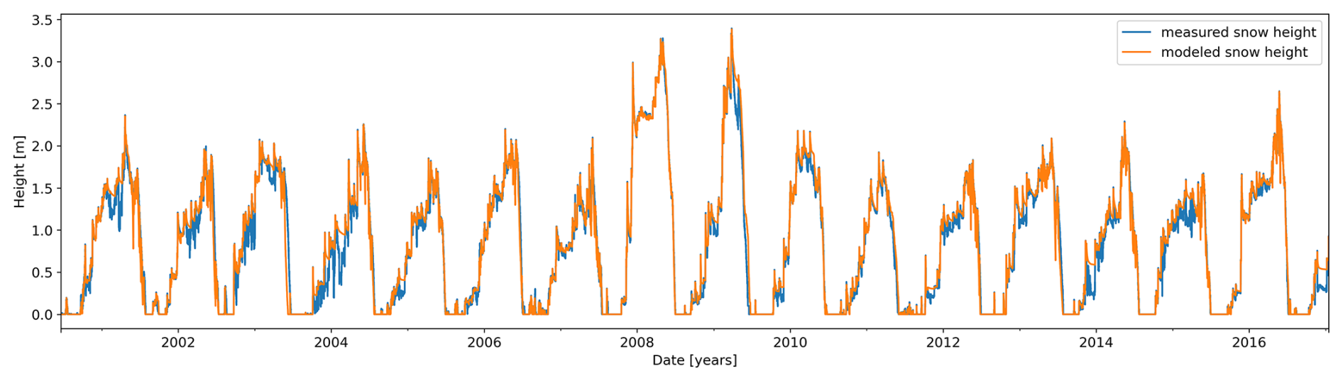
Figure A1 Time series of daily averaged measured and modelled snow height during natural undisturbed conditions at the Schilthorn site from 2000 to 2017.

A2 Ground temperatures

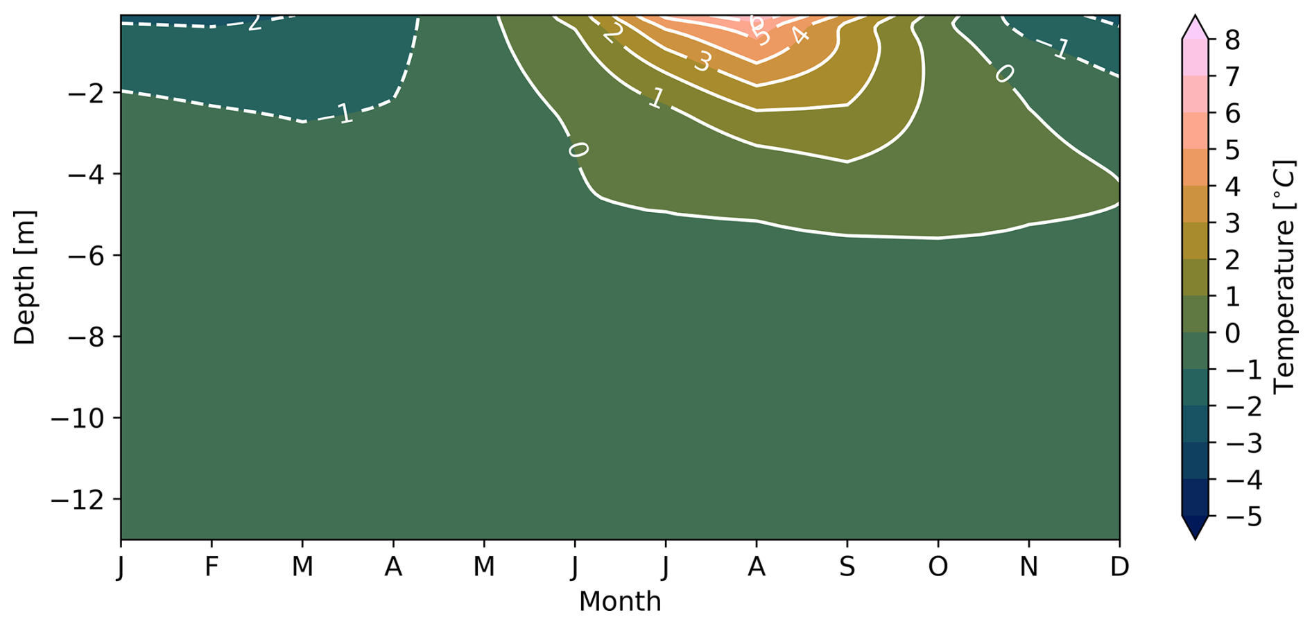
Figure A2 Monthly averaged modelled ground temperatures resulting from natural undisturbed conditions at the Schilthorn site from 2000 to 2017.

Appendix B: Thermal stabilization with thermal insulation

B1 Thermal insulation conductive heat flux distribution

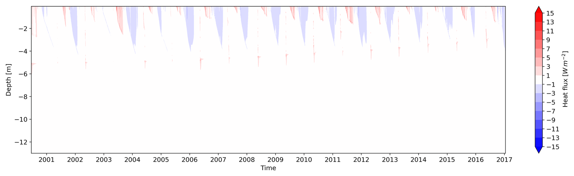
Figure B1 Time series of daily averaged modelled conductive heat flux from thermal insulation experiment using 50 mm thermal insulation layer at the Schilthorn site for the period of 2000 to 2017.

B2 Thermal insulation thickness effect

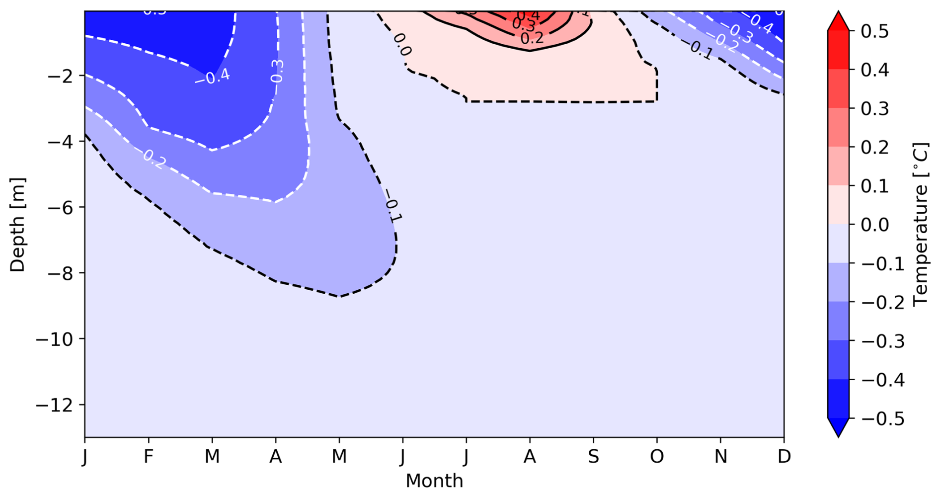
Figure B2 Monthly averaged temperature differences between 50 and 100 mm thermal insulation thicknesses.

B3 Heat flux attenuation distribution of conductive heat fluxes

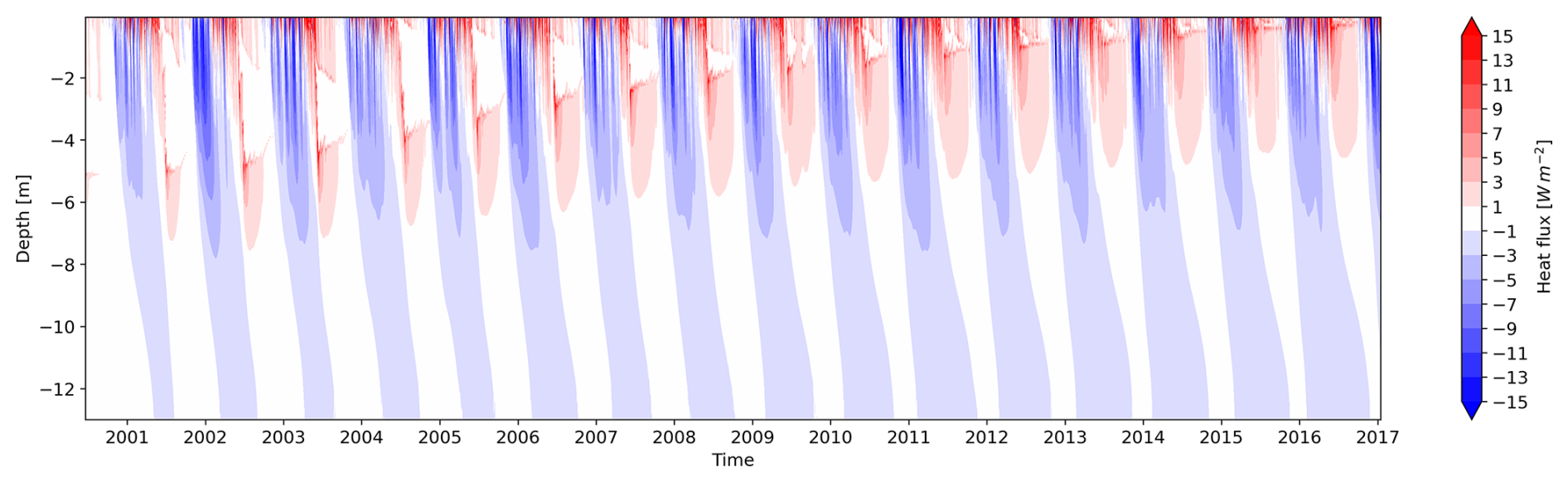
Figure B3 Time series of daily averaged modelled conductive heat flux from the heat transfer attenuation experiment at the Schilthorn site for the period of 2000 to 2017.

Appendix C: Thermal stabilization with active cooling

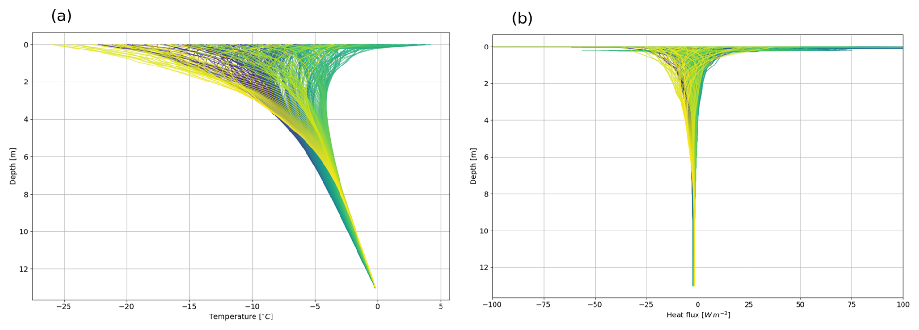
Figure C1 (a) Daily averaged temperature distribution, and (b) daily averaged heat flux distribution for the last year of the simulations, 2016 after 16 years of active cooling and shading.

Appendix D: Thermal stabilization methods comparison

Table D1 Thermal stabilization methods comparison.