Ground ice estimation in permafrost samples using industrial computed tomography and multi-sensor core logging and comparison to destructive measurements

Permafrost contains a variety of ground ice types (e.g., pore, segregated, intrusive, vein, or massive ice) that have a diversity of cryotextures which organize to form distinctive cryostructures. The distribution and abundance of those ground ice types determine the potential for thaw subsidence and terrain effects of permafrost landscapes. Analysis of permafrost samples allows improved understanding of ground ice formation and internal and external permafrost processes, as well as improved tools to predict thaw settlement and consolidation. However, most methods to characterize permafrost are destructive and of low resolution. Here, some of the limitations of traditional destructive methods are overcome using an industrial computed tomography (CT) scanner. We use this laboratory-based method to systematically characterize five permafrost samples. We visualize cryostructures, measure frozen bulk density, and estimate volumetric and excess ice contents non-destructively and compare these results with traditional destructive analyses at similar spatial scales.

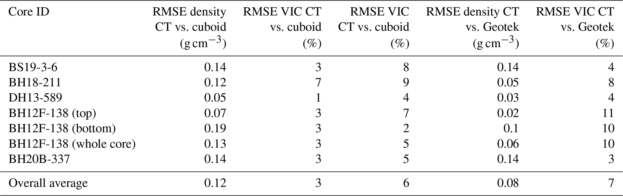
The results show strong agreement between traditional destructive analyses (RMSEs for density, volumetric ice, and excess ice contents are 0.12 g cm⁻³, 3 %, and 6 %, respectively) as well as recent developments using a multi-sensor core logger (MSCL) (RMSEs for density and volumetric ice contents are 0.08 g cm⁻³ and 7 %, respectively). These results demonstrate that these non-destructive approaches can produce consistent results and provide the added benefit of archiving images and enhancing digital permafrost datasets. The development of standardized and interoperable methods for permafrost characterization has the potential to build more robust permafrost datasets and strengthen efforts to understand future thaw trajectories of permafrost landscapes.

1 Introduction

Permafrost is rock or soil that has remained below 0 °C for at least 2 consecutive years. Within permafrost, several different types of ground ice can form: pore ice within the void spaces between soil or rock particles; segregation ice as distinct lenses formed through migration of water within permafrost; aggradational ice, a type of segregation ice that forms as the permafrost table rises; vein or wedge ice that forms within thermal contraction cracks; intrusive ice that forms when water is injected under pressure; or massive ice, which refers to relatively pure bodies of ice within permafrost (Subcommittee on Permafrost, 1988). These differing types of ground ice have distinctive associations of cryotextures, which refer to the appearance and characteristics of ice crystals, gas bubbles, and their interfaces with soil particles at a more microscopic scale, and cryostructures, which refer to the 3D patterns and arrangements of ice bodies within the frozen ground (such as layered, lenticular, or reticulate patterns) (Murton and French, 1994; French and Shur, 2010). Taken together, these ice-related features help identify the genesis of perennially frozen sediments and can provide insights into the conditions under which the permafrost formed, which can aid in understanding potential ground ice distribution. Of particular importance is excess ice – or ground ice that exceeds the natural pore volume that the sediment would have under unfrozen conditions (Brown et al., 1997; Zhang et al., 1999; Cai et al., 2020; Van Everdingen, 1998). When excess ice melts, it causes thaw settlement and ground subsidence, making its quantification increasingly critical as warming temperatures degrade permafrost across permafrost regions (e.g. Kokelj et al., 2013). Projections of widespread permafrost thawing by the end of this century (e.g. Cai et al., 2020) highlight an urgent need for standardized methods to measure and map excess ice distribution to better predict future landscape changes.

Cryostructural approaches to ground ice classification aim to understand permafrost development by systematically analyzing the shape, size, and spatial patterns of ice inclusions in frozen ground. These methods contrast with more commonly used engineering-focused descriptive systems, which rely primarily on visual descriptions and simple field tests, such as thawing samples to observe supernatant water content. While the descriptive approach provides practical field-based classifications useful for engineering applications, the cryostructural approach offers more process-based insight into permafrost formation processes and potential ground ice distribution, which is increasingly important for predicting thaw settlement and landscape response to climate warming (French and Shur, 2010).

Traditional approaches to permafrost characterization rely heavily on visual the description of exposures and cores (Kanevskiy et al., 2012; Stephani et al., 2014). While these approaches have advanced our understanding of permafrost, they require substantial experience of the analyst and are difficult to standardize. Quantitative methods typically require the destruction of samples to measure ice and moisture contents, which works well for ice-rich mineral soils but presents challenges for organic-rich materials where water may be retained in thawed samples. These limitations have driven the development of non-destructive methods like computed tomography (CT) scanning that can systematically analyze intact frozen cores, providing standardized, quantitative data on ground ice while preserving samples for additional analyses (Calmels and Allard, 2004, 2008; Calmels et al., 2010). This approach offers the potential to better understand permafrost formation, internal structure, and likely response to thaw while developing more consistent and interoperable methods applicable across different permafrost materials.

Micro-computed tomography (µCT), which offers much higher spatial resolution than conventional CT, has emerged as a promising solution to the limitations of traditional permafrost characterization methods since the pioneering work of Calmels and Allard (2004, 2008), who demonstrated its utility for measuring ice and gas contents in permafrost and linking these to processes of ground ice formation. Subsequent studies have expanded the application of µCT scanning to examine cryostructures (Calmels et al., 2010; Fan et al., 2021), excess ice (Lapalme et al., 2017), soil degradation in freeze–thaw cycles (Nguyen et al., 2019; Wang et al., 2018, 2024; Roustaei et al., 2022a, 2024), quantification of micro-lenticular ice lens formation (Darrow and Lieblappen, 2020), unfrozen water content (Roustaei et al., 2022b), soil–ice relations (Torrance et al., 2008), and permafrost composition (Nitzbon et al., 2020).

Although the method has been developed, there have been few systematic comparisons of high-resolution µCT scanning (<100 µm) with established methods for differentiating excess ice from pore ice across different permafrost materials. µCT typically offers very high spatial resolution (down to a few microns) for small samples, while industrial CT provides a balance of higher power and the ability to scan larger samples at slightly lower resolution, and medical CT is generally optimized for human-sized imaging at lower resolution and power. This study addresses this gap by using industrial CT scanning, which offers higher peak power and resolution than medical CT scanners, to analyze five different permafrost cores representing a range of typical properties (e.g., density and ice contents). We develop a new approach using an internal water standard to calibrate linear attenuation coefficients to real density values and systematically compare CT-derived measurements of frozen bulk density, excess ice, and volumetric ice contents with both destructive physical measurements and multi-sensor core logging (MSCL). We include a sensitivity analysis to examine how spatial resolution affects excess ice estimation. While our sample set does not capture the full heterogeneity of permafrost materials and ground ice abundance, it provides a rigorous test of CT methods for quantifying ground ice in common permafrost materials.

2 Methods and materials

2.1 Site and sampling

Five cores were investigated in this study, each representing common materials encountered in permafrost regions, such as silt (ice-poor and ice-rich), peat, silty peat, and diamicton (a coarser, mixed-grain material), and containing a relatively simple vertical cryostratigraphy to minimize the impact of lateral heterogeneity (Table 1). Minimizing lateral heterogeneity is important because such variations can introduce noise when comparing multiple data acquisition methods applied to different, but nearby, sample volumes within the same core (Fig. 1). This consideration and its implications are explained further by Pumple et al. (2024), who discuss how variations in measured densities of permafrost cores may reflect real heterogeneities in physical properties or artifacts introduced due to core preparation or mounting of frozen materials.

Table 1 Sampling location and physical properties of cores analyzed in the study. N/A – not applicable.

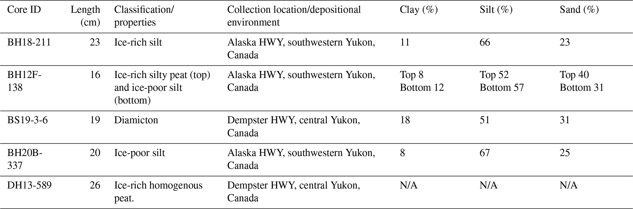
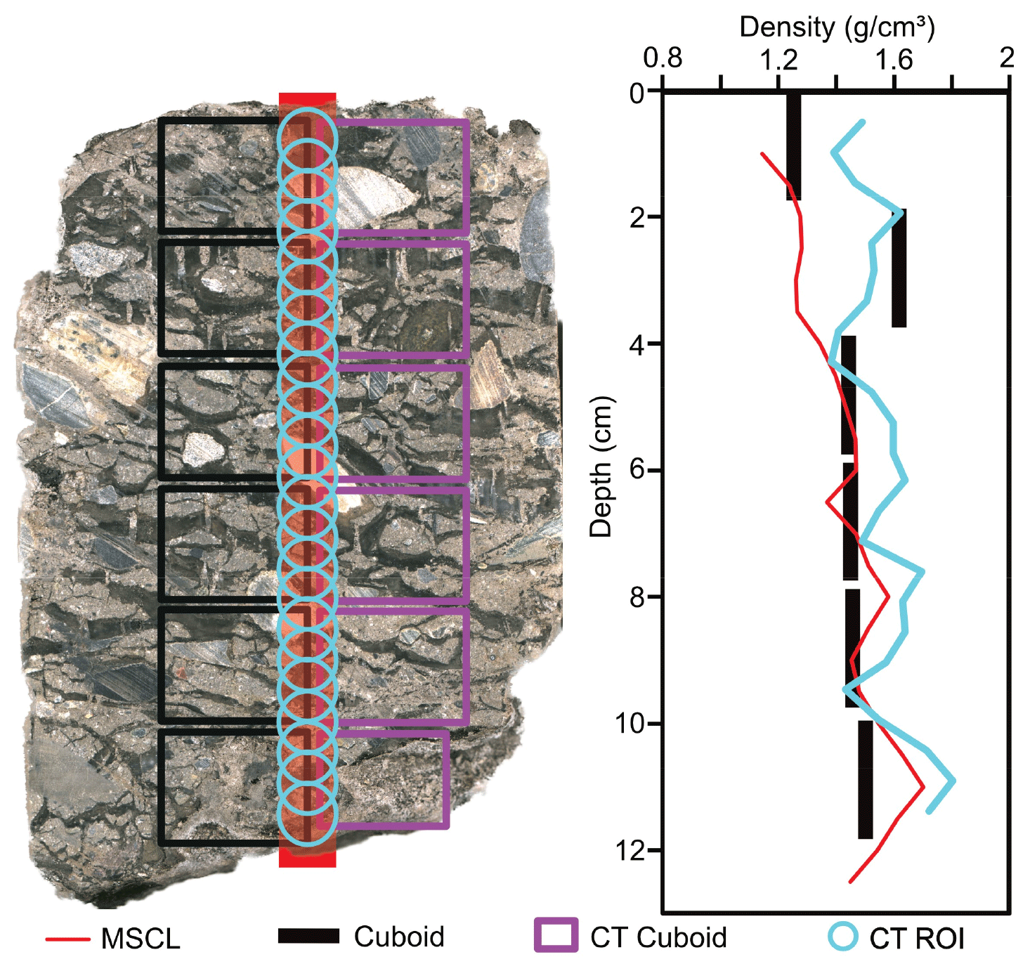
Figure 1 Image of a core highlighting the destructive subsample locations relative to the non-destructive data collection transects (black: subsampled cubes for destructive measurements; purple: subsampled cubes for CT scans).

These cores were collected during two separate field campaigns in 2013 and 2019 with some cores being collected in southwestern Yukon along the Alaska highway (HWY) and other in central Yukon along the Dempster HWY. All cores were collected in a sub-arctic setting. Following extraction, the cores were bagged, labelled and stored at subzero temperatures via a pre-chilled cooler, and quickly transported to the field base where a chest freezer was present. The chest full of cores was then transported to the Permafrost ArChives Science (PACS) Laboratory and archived into walk-in archive freezer space. Samples were prepared for two different stages: non-destructive scans and destructive physical measurements. As such for the non-destructive scans, physical cores were cut in half and run through all non-destructive data collection methods. For the second stage, a duplicate transect of cuboid samples was collected from the middle of the core to allow non-destructive data analysis at a higher resolution on one set of the subsampled cubes. As seen in Fig. 1, this resulted in the cuboids flanking either side of the MSCL and CT results which were collected from a central transect on the half-core samples.

2.2 Industrial micro-computerized tomography

Micro-computed tomography (µCT) is a non-destructive technique that has been useful in the investigation of geological porous media (Ashi, 1997; Ketcham and Carlson, 2001; Kozaki et al., 2001; Flisch and Becker, 2003; Calmels and Allard, 2004; Van Geet et al., 2005; Tanaka et al., 2010; Nitzbon et al., 2022). This imaging method captures radiograph images through the production of X-rays which pass through a cabinet and are recorded by the detector panel opposite the source. The sample is placed between the source and the detector panel, and the resulting relative absorption of the X-rays energy is recorded by the detector panel creating the radiograph image. To collect a 3D image, a set of 2D X-ray radiographs are collected at multiple angles and secondly reconstructed to form a 3D image. The final measurement unit, commonly visualized as a histogram, is the linear attenuation coefficient, which depends on both the density and the electron density of the material (Ketcham and Carlson, 2001).

The scans presented here were captured using a helical scan with a Nikon XTH 225 ST cabinet-based industrial computed tomography micro-CT scanner. The system uses an electronically adjustable 225 Kv 225 W power source (Fig. 2). This system includes both a tungsten rotating reflection target source and a tungsten fixed reflection target source coupled with a 16 bit 2000 × 2000 pixel detector capable of a focal spot size range of 3–121 µm depending on the size of the area of interest and size of the object being scanned. The 10 cm diameter frozen permafrost half cores were scanned with the reflection target source at 200 Kv 35 µa with an exposure time of 125 ms and a voxel (3D volume element representing pixel resolution and slice thickness) size of 65 µm. Scan times ranged from 30 to 45 min per core, with a maximum height of ∼ 12 cm scanned per core due to vertical stage movement limitations and inclusion of calibration materials. The subsampled cubes from the cores were scanned with the rotating reflection target source at 225 Kv 133 µa with an exposure time of 125 ms and a voxel size of 25 µm. Scan times for the subsampled cubes were 30 min per cuboid. The images were reconstructed into 3D grey-scale volumes using the Nikon CT pro 3D software and analyzed using ORS Dragonfly 2022 image processing software (ORS, 2021).

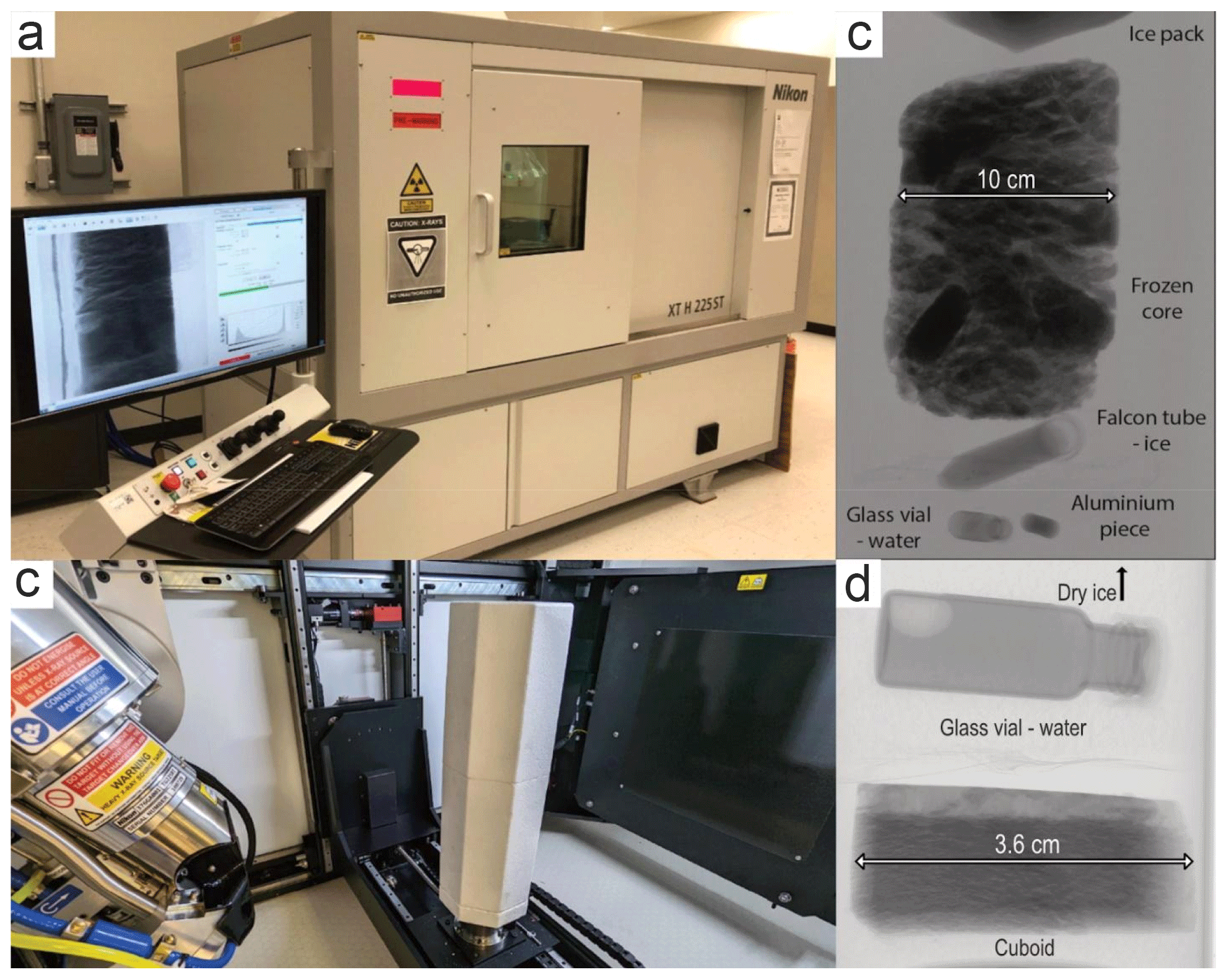
Figure 2 (a) The CT scanner of the PACS Laboratory. (b) The internal setup for the core scan. (c) X-ray image of the internal setup of the core. (d) X-ray image of the internal setup of the cube.

An insulated sample holder was developed for this project to ensure samples remained frozen during CT scanning. Both cubes and cores were housed in the same style of styrofoam container; however, the internal setup varied due to the size of the sample under investigation. Full cores were taken from a nearby chest freezer and placed vertically into a larger container (12 cm inner diameter) with a −80 °C ice pack positioned directly above (Fig. 2b and c). In contrast, the cubes were placed in smaller containers (9 cm inner diameter), held in plastic vials beneath a foam divider, and cooled with dry ice on a perforated foam layer to circulate cold air over the sample (Fig. 2d). These configurations were tested in advance using internal, surface, and air temperature probes, confirming that both setups maintained sub-zero temperatures for the full scan duration. It should also be noted that full core scans produced partial results due to vertical stage height limitations in the CT scanner. While the scanner can hold samples up to ∼ 30 cm wide by 35 cm high, the maximum scan height depends on voxel resolution and sample width. This limitation was resolved once the cores were subsampled for destructive testing. As a result, for some cores, such as the peat core, it was not possible to compare full vertical data sets across MSCL, CT, and destructive methods.

2.2.1 CT calibration

The linear attenuation coefficient (μ) represents the energy attenuated within a single voxel volume, while the voxel population is the population of voxels within a scan volume (Ketcham and Carlson, 2001). By creating a histogram (linear attenuation coefficient vs. voxel population) with these values, distributions of relative grey values can be presented. If uncalibrated, the resulting grey values observed in the histogram of a CT scan appear as linear attenuation coefficients. The medical field has developed methods for converting linear attenuation coefficients to Hounsfield units, and as a result, the Hounsfield unit has become commonly used in CT research (Hounsfield, 1973; Wellington and Vinegar, 1987; Duliu, 1999; Knoll, 1999; Ketcham and Carlson, 2001; Duchesne et al., 2009). Lee et al. (2015) took it one step further and converted mean Hounsfield unit values to bone mineral density values (mg cm⁻³) via a linear regression analysis. A similar approach was used in this study by collecting the CT scans with an internal standard of known density (water) later used to calibrate the resulting linear attenuation coefficients into g cm⁻³ using the Nikon CT Pro 3D software (CT Pro version 5.4). It should be noted that all cores were scanned with ice, water, and aluminium calibration pieces of which water proved to be in closest agreement with destructive analyses. The water and aluminium were located outside of the insulated container during the core scans to avoid freezing. The cube scans had only the water located directly above the cube sample but isolated from the sample and dry ice by insulated foam to minimize the exposure to the cold air temperature within the developed insulated container. The aluminium calibration piece generally underestimated the bulk density, while the ice calibration piece resulted in a slight overestimation. Aluminium was chosen for its consistent density of 2.71 g cm⁻³ representing an upper limit of the expected bulk density within the selected materials. The ice calibration was a 15 mL falcon tube filled and frozen at −5 °C to minimize expansion issues and bubbles. Overall the water calibration produced the most accurate results apart from ice-poor sediments. The Nikon CT Pro 3D software uses a linear two-point calibration with the first fixed point being air (equal to zero) and the second a user-defined value based on a user-selected pixel population. A representative (local) population of pixels was selected from our water sample in a 2D slice of the scan and informed the expected average target value (1 g cm⁻³). This results in displaying grey values in g cm⁻³. These densities can then be presented in a histogram, the shape of which reflects the volumetric content of the components in the sample (Calmels et al., 2010).

2.2.2 Image processing

Image preprocessing usually consists of two main stages: (1) selection of the region of interest (ROI) or (2) segmentation. In this study both stages were done using Dragonfly software (ORS, 2021). This software enabled us to process the 3D reconstructed X-ray tomographs of the frozen materials to segment, quantify, calculate, and illustrate the cores' physical properties. For the first stage, a series of ROIs were created in the half-core CT results down the central vertical axis of the cores to mimic the data collection points of the MSCL as presented in Pumple et al. (2024). Figure 1 displays the relative location of these ROIs which were sized to match the spot size of the gamma ray at the surface of the core, ∼ 10 mm in diameter. The central point of each ROI was placed 5 mm apart, resulting in a significant overlap between adjacent data points, again similar to the data collection process for the MSCL. In this study, all cores were calibrated so the histogram values were displayed in g cm⁻³. Following calibration, the histograms served not only as visualization tools but also as a means to extract quantitative information. To extract the frozen bulk density from each ROI, the mean grey values were extracted in calibrated density values (g cm⁻³).

The second stage, segmentation or the ability to differentiate materials, depends on their respective linear attenuation coefficients, meaning materials with divergent densities and/or atomic numbers are easier to differentiate (Kyle and Ketcham, 2015). Analyzing a multi-modal histogram of a CT image is straightforward for material differentiation, while materials with similar unimodal density distributions may appear as a single peak in the histogram (Wang et al., 2024). In addition to the relative density of the scanned materials, the image resolution or voxel size also directly impacts the image segmentation process. The voxel size can impact the image segmentation through the partial volume effect which relates directly to the resolution or voxel size of the scan and for geological samples to grain size, minimal pore size, and organic content (Soret et al., 2007; Nitzbon et al., 2022).

In this study, an automatic image thresholding method named “Otsu ” was used. The algorithm of this method, proposed by Nobuyuki Otsu (1979), performs automatic clustering-based image thresholding, assuming that there are two classes of pixels which are “foreground” and “background” pixels of the image. The optimum thresholding is calculated by distinguishing the two classes so that the minimum class variance is obtained (Kumar and Tiwari, 2019). This method was applied to the selected regions of interest from stage one to differentiate sediment and ice. In each image processing step, we tried to isolate the materials within our scans based on density and slowly slice away the lighter density portion (ice) until we were certain we had collected the target material range (often a mixture of ice and sediment). Figure 3 shows the ice (less dense material) being segmented from the surrounding sediment through multiple image processing steps using the Otsu method where only the background (less dense) portion of the previous step is added to the final result. This approach shows that applying the first image processing step will mainly extract the visible ice, while using multiple Otsu analyses additional lower-density ice-rich mixtures (mainly pore ice) are extracted, e.g., the area shown inside the red circle of Fig. 3b–d. Note that all the above-mentioned segmentation steps can also be done by visual inspections instead of the automatic thresholding method, but it can vary significantly between users, leading to inconsistent results.

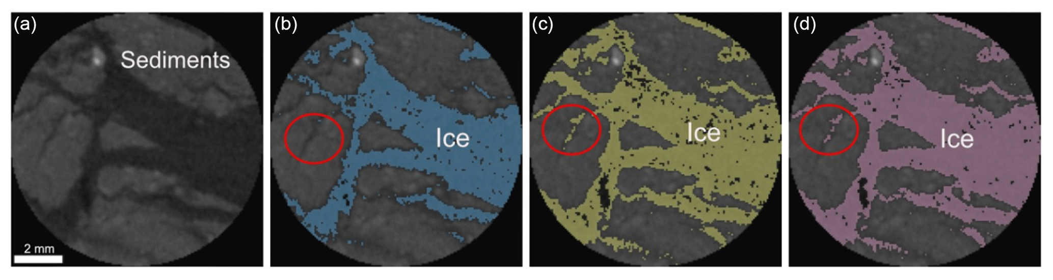
Figure 3 Overview of a slice from ice-rich silt core (a) before image processing, (b) after the first step, (c) after the second step, and (d) after the third step of image processing using the Otsu method.

2.3 Physical density measurements

Ground ice content is typically expressed either as the gravimetric moisture / ice content (the ratio of the mass of the ice in a sample to the mass of the dry sample) or as the volumetric moisture / ice content (the ratio of the volume of ice in a sample to the volume of the whole sample) (Van Everdingen, 1998). Excess ice refers to the amount of ice in the soil that exceeds the volume of the pore space in the unfrozen state (Subcommittee on Permafrost, 1988). Similar to thaw-strain measurements in geotechnical investigations (Shur, 1988; Pullman et al., 2007; Kanevskiy et al., 2012), Kokelj and Burn (2003) and O'Neill and Burn (2012) both applied a method for destructively extracting excess ice content measurements from frozen samples. This method includes the complete thaw, homogenization, and settling time of the sample to extract the supernatant water content and estimate excess ice content. Their method does not require measurement of frozen sample volume since the volumes of sediment as well as the supernatant water should be recorded from the graduated beakers containing the samples once completely thawed. The excess ice content (E_i) of the samples can then be estimated by the following equation (Kokelj and Burn, 2003):

$$\begin{array}{}\text{(1)}& \left(E_{\mathrm{i}}\right)={\displaystyle \frac{\left(\mathrm{Wv}\times \mathrm{1.09}\right)}{(\mathrm{Sv}+\mathrm{Wv}\times \mathrm{1.09})}}\times \mathrm{100},\end{array}$$

where Wv is the volume of supernatant water (cm³), multiplied by 1.09 to estimate the equivalent volume of ice, and Sv is the volume of saturated sediment (cm³).

This study takes an approach similar to Kokelj and Burn (2003) in that the supernatant moisture content is destructively assessed in order to calculate excess ice content. However, since the volume of soil samples was precisely measured through the following steps (Pumple et al., 2024), volumetric ice contents were also measured.

To independently assess density and ice content measurements and also be able to perform scans at higher resolutions, the cores were subsampled as 2 × 2 × 4 cm cubes. The subsampling process was done in a walk-in freezer maintained at −7 °C. The initial step involved removing material from the outer edges of the whole core that might have thawed during coring or been affected by sample storage. Core segments were split lengthwise with a rock saw equipped with a 35 cm diameter diamond cutting wheel. Cuboid aliquots were cut from one half of the split core, while the other half was retained as an archive. The rounded edges were removed from the half core to expose an internal slab. For this study, a duplicate set of cuboids was obtained by cutting the internal slab in half. Approximately 3 cm³ aliquots were subsampled from the cores for samples with low ice contents to ensure that the cuboids did not fracture or disintegrate during sampling. Digital callipers (±0.01 mm) and a digital analytical balance (±0.01 g precision) were used to measure physical dimensions and mass, respectively, to calculate the frozen bulk density. The cuboids were then thawed at room temperature for 24 h in glass beakers covered with Parafilm to minimize evaporative loss. Excess moisture was removed from the beakers containing the thawed samples, and the sample weight was recorded again to calculate excess moisture content. The cuboids were then dried in an oven for 24 h at 105 °C and reweighed to determine both volumetric ice content and gravimetric moisture content. Finally, the remaining dried material was heated at 550 °C for 4 h to determine the percent organic content via loss on ignition. High organic content could result in water absorption by soil matrix upon thaw and more complexity in the measurements of excess ice contents.

Because in some soils, such as peat, excess ice will be absorbed by the soil skeleton upon thaw (Johnston, 1981), the Kokelj and Burn method was adjusted for samples with high organic contents by applying a slight pressure on the thawed cube and extraction of the released water. Additionally, the organic content of each sample was measured via loss on ignition (LOI) (Heiri et al., 2001). The cuboid method, described by Bandara et al. (2019), is similar to other volumetric and gravimetric methods used to measure bulk density and ice content but takes advantage of the frozen state of the material, which allows for a greater accuracy of volume measurement. Processing is undertaken in a walk-in freezer following methods outlined in Pumple et al. (2024).

2.4 Multi-sensor core logger (MSCL)

The PACS Laboratory MSCL is a floor-mounted, automated logging system, manufactured by Geotek, which can be used to analyze whole or split cores. This core logger is equipped with two magnetic susceptibility instruments, a line-scan camera and a caesium-137 (¹³⁷Cs) gamma source and detector which provides measurements of gamma attenuation. Pumple et al. (2024) provides additional details on the methods used for the MSCL data collection and calibration. This analysis yields key physical parameters such as frozen bulk density and volumetric ice content derived from gamma attenuation measurements combined with soil density estimates and established equations (Lin et al., 2020). We used the density and volumetric ice content results reported by Pumple et al. (2024) as an established non-destructive reference technique to validate and compare with our own ice content estimations.

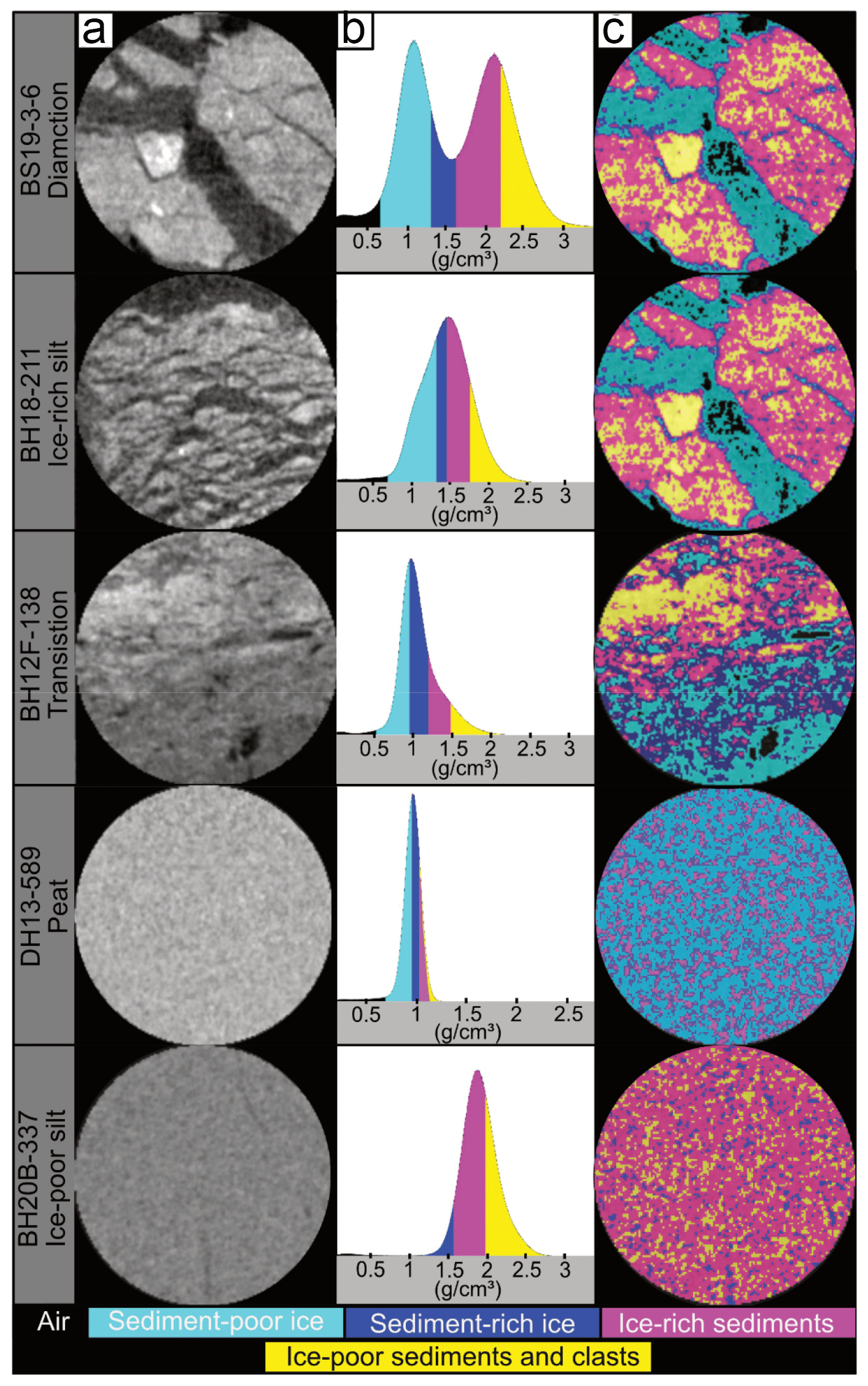
Figure 4 (a) Overview of slices from the permafrost cores before image processing, (b) histograms, and (c) image segmentation results.

3 Results and discussions

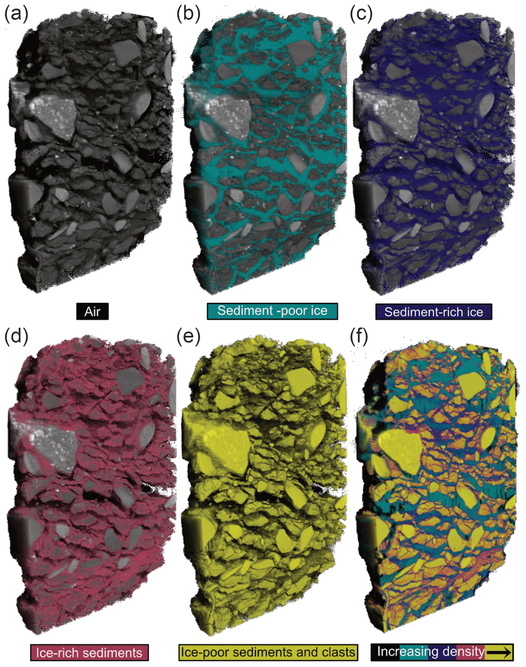
Figure 4a and b show one slice of a small ROI and its histogram from five different cores of this study. The differences in the shapes of the histograms are due to the different sediment densities. The diamicton core has the highest sediment density and a bimodal histogram in which the first mode represents ice and the second is related to the sediments and clasts, whereas in the other cores, ice and sediment appear as a single mode. Image segmentation of these slices using the Otsu method resulted in the differentiation of five different classes of ice / sediment ratios on the basis of their relative densities: air, low ice or sediment-poor ice, high ice or sediment-rich ice, low sediment or ice-rich sediments, and high sediment or ice-poor sediments or clasts shown in Fig. 4b and c. Low ice comprises primary visual or excess ice; high ice mainly results from extraction of pore ice or ice proximal to sediment (sediment-rich ice). It should be noted that the pore ice inclusions within the mineral soil matrix are often smaller than the spatial resolution of the CT and the resulting grey value of a voxel is related to the mixture composition of low-density ice and high-density mineral grains. This phenomenon, called partial volume effect, is the main reason why the high ice appears denser. Low-sediment and high-sediment categories differentiate ice-rich sediments from sediments with lower and higher densities, respectively. Figure 5a–f illustrate the image segmentation results for the whole diamicton core, highlighting these distinctions.

Figure 5 Image segmentation results of the diamicton core.

3.1 Core results

3.1.1 Ice-rich silt core (BH18-211)

Figure 6 shows the destructive (cuboid) and non-destructive (CT and MSCL) results of the ice-rich silt core, illustrating that the CT frozen bulk densities are in strong agreement with both the cuboid (RMSE = 0.12 g cm⁻³) and MSCL (RMSE = 0.14 g cm⁻³) results. This core has a high organic content (8 %–19 % organic), micro-lenticular and layered cryostructures, and 66 % silt. Cuboid physical EIC and VIC (excess and volumetric ice content, respectively) measurements range from 19 %–34 % and 68 %–76 %, respectively, while the CT EIC and VIC estimates range from 20 %–68 % and 32 %–74 % at the same depths where cuboid measurements were collected. The 65 µm EIC (red line in Fig. 6c) shows good accordance with the cuboid EICs (RMSE = 9 %) apart from the ice layer where the cuboid's relatively low sample resolution results in an averaging out of the ice content across the ice layer. The 65 µm CT VICs (black line in Fig. 6c) illustrate the resolution limitation in extracting the pore ice of this sandy silt core, while the 25 µm VICs shown as black cubes in the same plot tackle this limitation and agree well with VICs extracted with the cuboid method (RMSE = 7 %). The MSCL VICs follow the same trend as the cuboid data (Fig. 6c) but consistently tend toward lower values in the ice-poor regions.

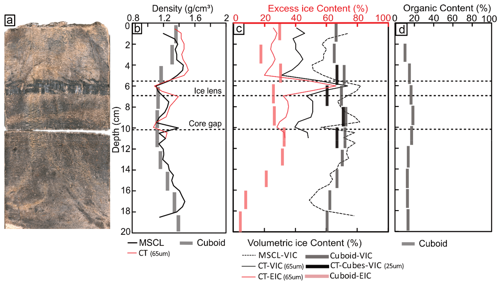
Figure 6 (a) MSCL image of the ice-rich and organic-rich silt core, (b) bulk density, (c) ice contents, and (d) organic content distribution in core depth.

3.1.2 Transition core (BH12F-138)

Figure 7 shows the results of the transition core from both destructive (cuboid) and non-destructive (CT and MSCL) methods, illustrating a sharp boundary between an ice-rich silty peat, containing massive and rare crustal cryostructures, and an ice-poor inorganic silt with a mainly micro-lenticular cryostructure. The organic content of the core's top section, ranging from 53 %–71 %, highlights this transition (Fig. 7d). Cuboid physical EIC and VIC measurements range from 6 %–28 % and 64 %–88 %, respectively, while the CT EIC and VIC estimates range from 9 %–33 % and 42 %–95 % at the same depths where cuboid measurements were collected. This figure also shows that the CT bulk density results are in strong agreement with both the cuboid (RMSE = 0.13 g cm⁻³) and gamma attenuation data (RMSE = 0.06 g cm⁻³), in agreement with the results reported by Pumple et al. (2024). The 65 µm EIC results (red line in Fig. 7c) follow the cuboid results (RMSE = 5 %) in the silty section. The 65 µm VIC (black line in Fig. 7c) resolves more than 50 % of pore ice, while the higher resolution (25 µm, black cubes in Fig. 7c) estimates up to 100 % (RMSE = 3 %).

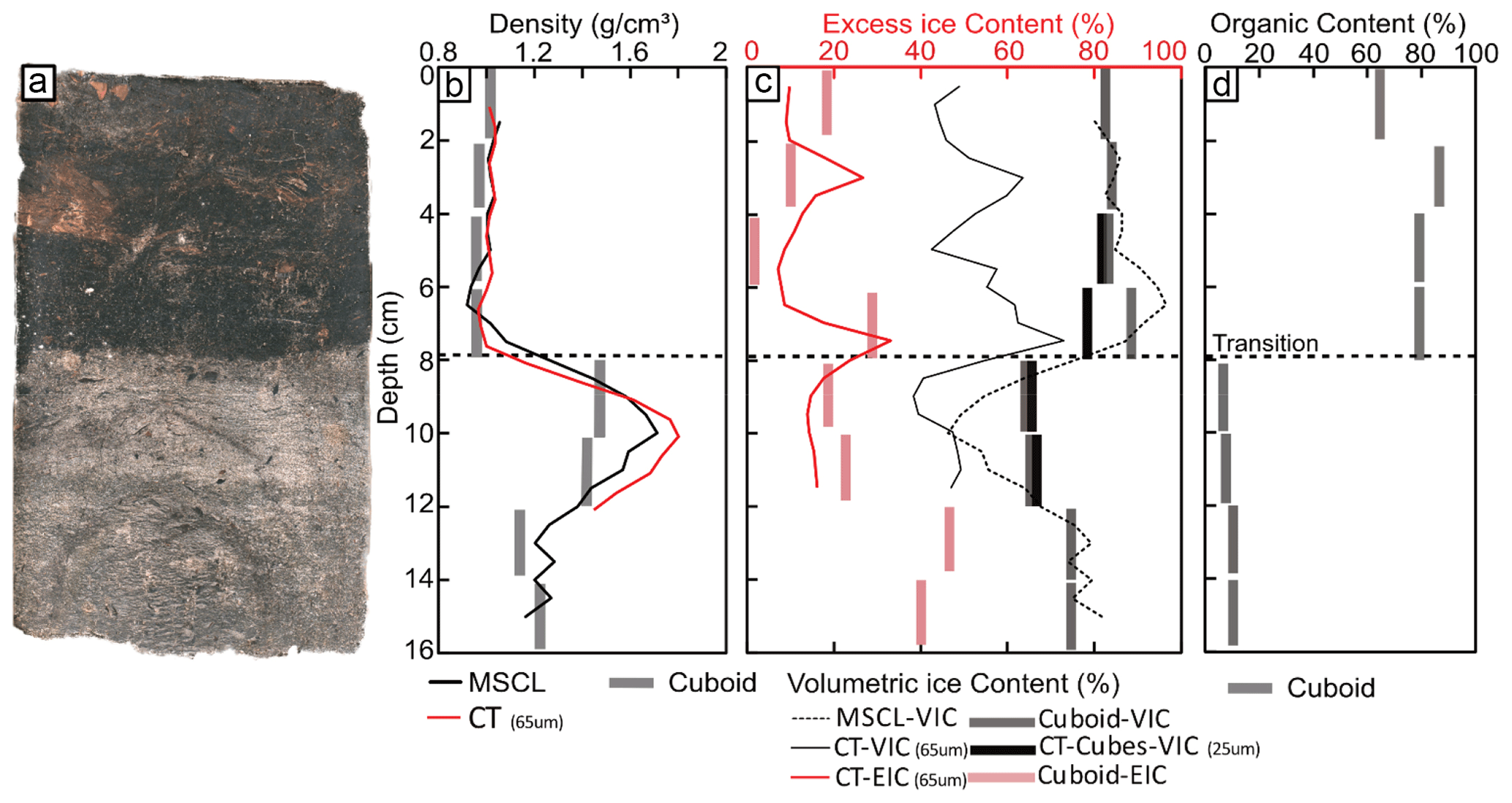
Figure 7 (a) MSCL image of the transition core, (b) bulk density, (c) ice contents, and (d) organic content distribution in core depth.

3.1.3 Diamicton core (BS19-3-6)

Figure 8 illustrates the destructive (cuboid) and non-destructive (CT and MSCL) results of the diamicton core. This ice-rich diamicton contains both suspended and crustal cryostructures and more than 50 % silt (Table 1). Overall the bulk density and ice measurements from CT display high concordance with the gamma attenuation (RMSE = 0.14 g cm⁻³) and cuboid (RMSE = 0.14 g cm⁻³) methods (Fig. 8). Cuboid physical EIC and VIC measurements range from 30 %–50 % and 48 %–66 %, respectively, while the CT EIC and VIC estimates range from 22 %–57 % and 36 %–77 % at the same depths as the cuboid measurements. The 65 µm EIC results (red line in Fig. 8c) follow the cuboid results (RMSE = 8 %). The only point where the datasets differ notably is at 2–4 cm depth where the MSCL values shifts towards lower densities due to the core's lateral heterogeneity while the CT density still lines up well with the cuboid results. The ice contents of this cube are also much lower than CT and MSCL results. This is due to the collection procedure of the cubes which were just off-center to accommodate a duplicate run of cubes down the middle of the core for CT imaging and destructive measurements (as shown in Fig. 1). This single cube highlights the effect of differences in the locations of ROIs between CT/MSCL and the cuboid methods. Moreover, at this depth in the core cuboid sample, there was a clast which resulted in a local density high and lower ice content.

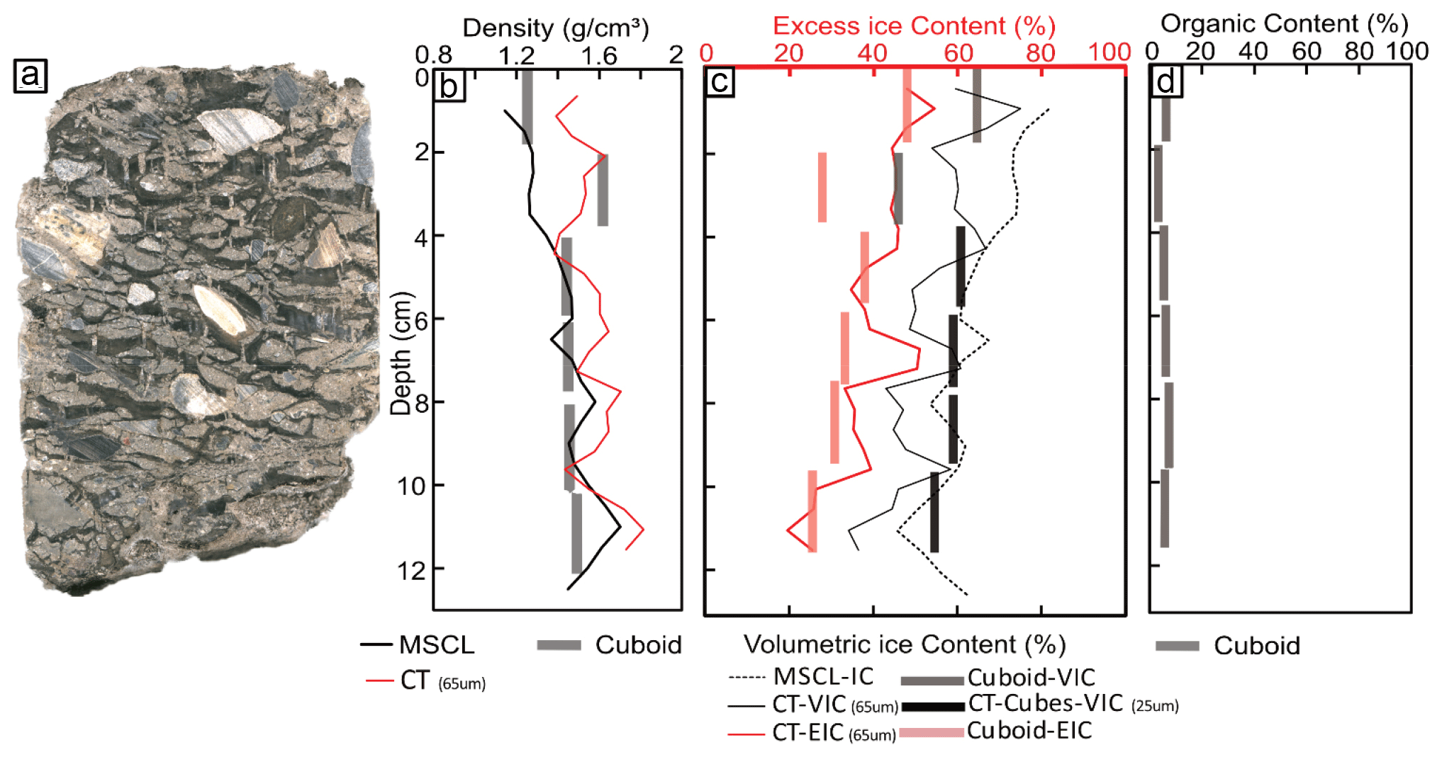
Figure 8 (a) MSCL image of the diamicton core, (b) bulk density, (c) ice contents, and (d) organic content distribution in core depth.

In this core, the 65 µm VICs agree well with the cuboid VICs, MSCL (RMSE = 4 %) ice contents, and 25 µm cube scan results (RMSE = 3 %) while in the transition core, the 65 µm VICs underestimated the other VIC results. The difference between the 65 µm VIC results and other VIC results for all cores except the diamict could be a result of the sample's grain size as the diamict has high clay content (∼ 18 %) relative to the other cores (∼ 8 %–12 %) (Table 2).

Table 2 Root mean square error results for the comparison between the CT/cuboid and MSCL VIC, EIC, and density measurements.

3.1.4 Ice-poor silt core (BH20B-337)

Figure 9 shows the results of the ice-poor silt core from both destructive (cuboid) and non-destructive (CT and MSCL) methods, illustrating a massive (non-visible) cryostructure within this inorganic silt that highlights the relatively low overall ice content throughout the core. This core has little variability throughout its profile. The CT bulk densities are consistent with both the cuboid (RMSE = 0.14 g cm⁻³) and gamma attenuation data (RMSE = 0.14 g cm⁻³). The 65 µm EIC results compare well with the cuboid EIC results (RMSE = 5 %), while the 25 µm cube scan ice contents show strong agreement (RMSE = 3 %) with the volumetric cuboid ice content estimates. It should be noted that based on the EIC results of 65 µm scans, the core has a small percentage of ice (around 5 %) in the form of microstructures beyond the natural pore space within the host sediment. However, upon thawing, the surrounding sediment absorbs the moisture into the available pore space, resulting in no EIC during the destructive analysis.

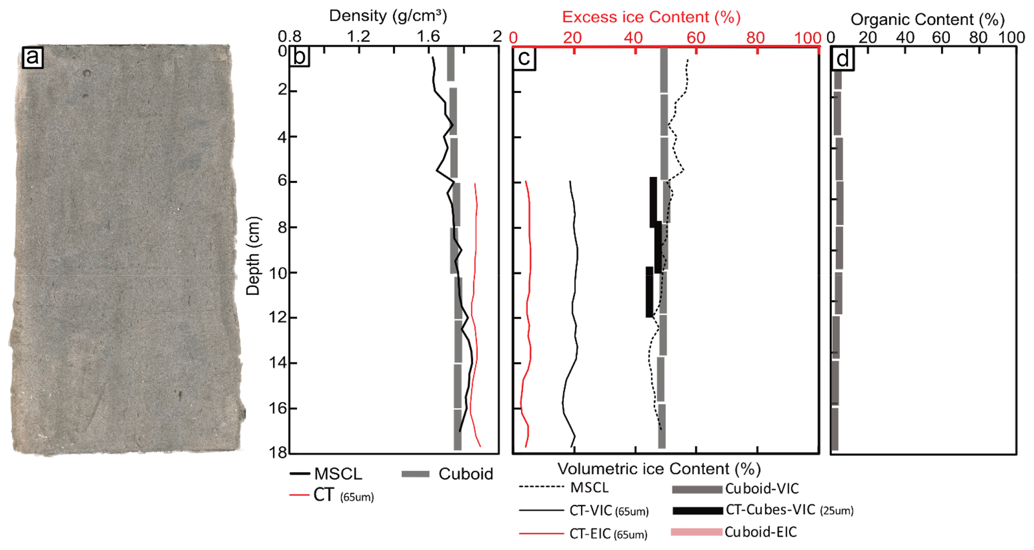
Figure 9 (a) MSCL image of the ice-poor silt core, (b) bulk density, (c) ice contents, and (d) organic content distribution in core depth.

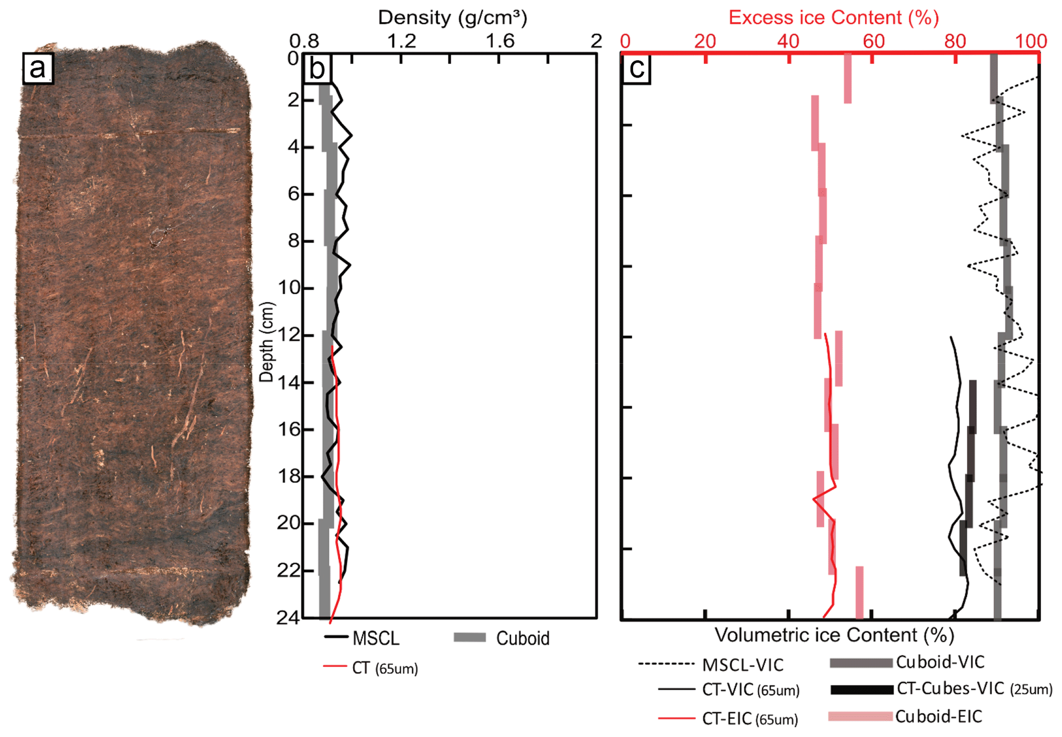
3.1.5 Peat core (DH13-589)

Figure 10 illustrates the destructive (cuboid) and non-destructive (CT and MSCL) characterization results of the peat core, with little variability throughout its profile. The core is formed of homogenous organics, with an organic-matrix cryostructure of visible ice within the densely packed peat. The CT bulk density results are similar to both the cuboid (RMSE = 0.05 g cm⁻³) and gamma attenuation results (RMSE = 0.03 g cm⁻³) (Fig. 10). The 65 µm ice content results (39 %–48 % of EIC) are also in accordance with the cuboid excess ice results (RMSE = 4 %). The 65 and 25 µm VICs are both showing good estimates of VICs (RMSE = 1 %). It should be considered that the adjusted method for the extraction of supernatant water, using slight pressure to release water from the organic matrix, was applied to the cubes of this core. As was previously discussed, this pressure will release the excess water that was absorbed by the peat skeleton upon thaw (Johnston, 1981).

Figure 10 (a) MSCL image of the peat core, (b) bulk density, and (c) ice contents.

3.2 Sensitivity analysis

In this study in order to do a sensitivity analysis and investigate the impact of resolution on the delineation between ice and sediment, repeat scans were conducted on the same cube. Initially, the half cores (10 cm diameter) were scanned with a 65 µm voxel size. This was due to the physical size (width) of the imaging window. The smaller size of the cubes, however, presented an opportunity to collect data from the same material but at a resolution of 25 µm. Some of the cubes were also scanned at the same 65 µm resolution as the half cores to make a direct comparison. Figure 11 shows the same slice location and orientation from the same cube at two different resolutions.

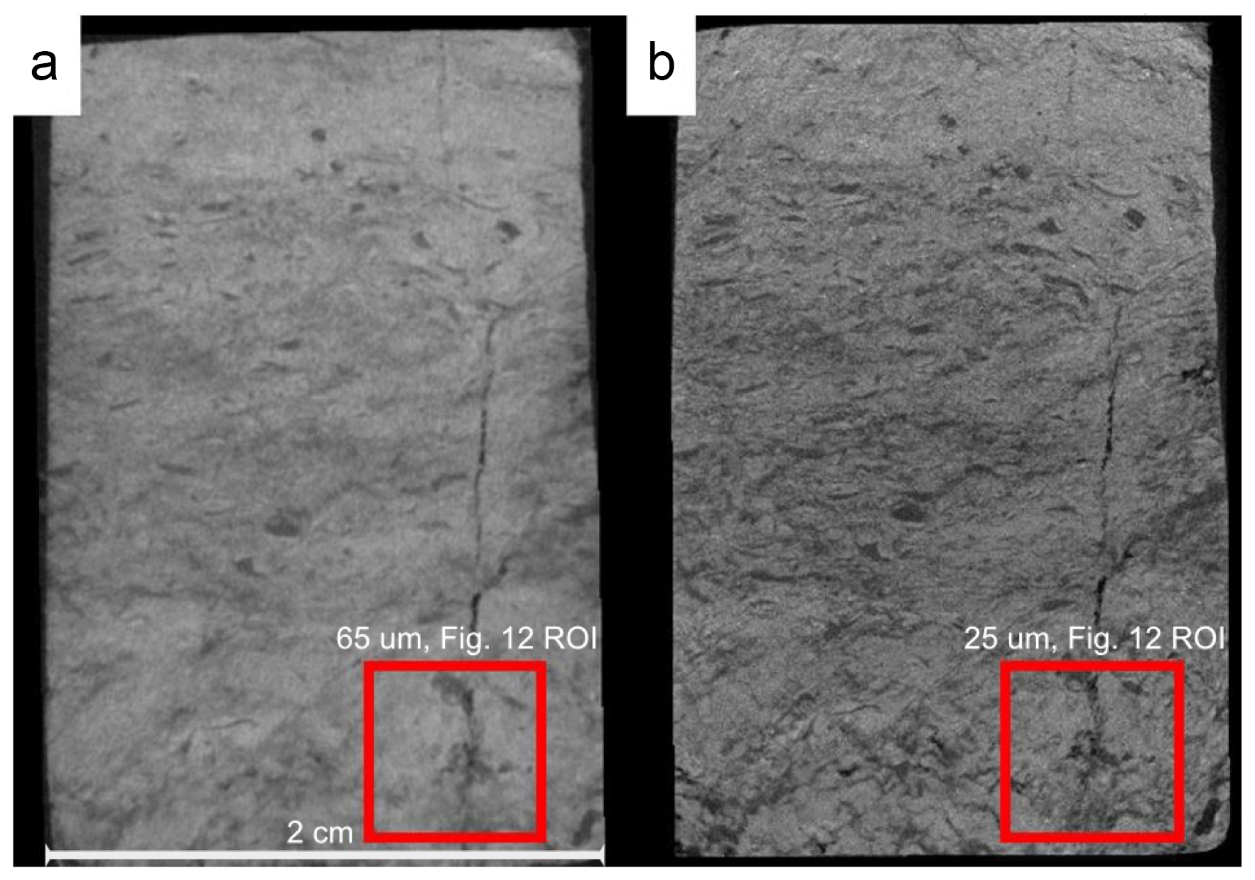
Figure 11 CT images of a cube (BH12F-138-10-12 cm) from the transition core at 65 µm (a) and 25 µm (b).

An ROI, shown as a red square in Fig. 11, was then selected in each CT-scanned cube to make a direct comparison between the delineated (Otsu split) ice contents from image processing and the ice contents determined from the destructive cuboid analysis of the corresponding cube sample. As reference points, the cuboid ice content results for this cube were as follows: 22 % excess ice and 65 % volumetric ice contents. Figure 12 shows the collected data from repeat image processing steps using the Otsu method of each cube scanned at both 25 and 65 µm resolutions as well as the cuboid results. The initial image processing steps for both the 25 and 65 µm scans closely capture the expected value of the EIC. However, only the 25 µm cube captures a representative value relative to the cuboid data for the measured volumetric ice content. This value is reached after six image processing steps using the Otsu method. These results illustrate the capability of 25 µm resolution for better extracting trapped ice inside pore spaces of this sandy silt sample, which could be due to the smaller size of pores than the resolution. The nature of the curve suggests that VIC cannot be delineated from the 65 µm resolution scans; however EIC is possible.

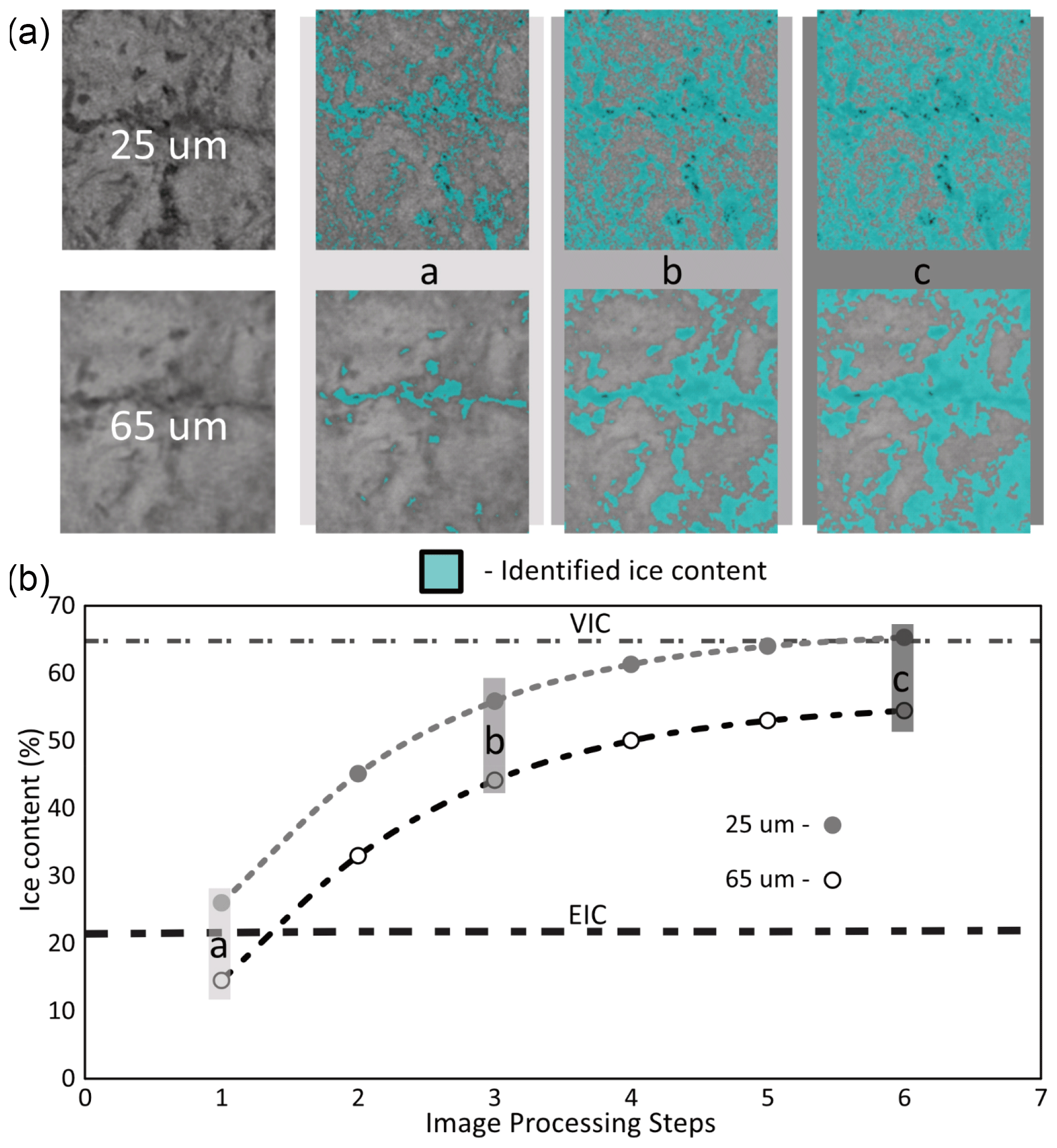
Figure 12 (a) CT ROIs taken from the 65 and 25 µm cube scans (BH12F-138-10-12 cm). (b) Identified ice contents at each image processing step using the Otsu split method.

Additionally, there is an observable increase in the amount of pore space or gas captured at the 25 µm resolution relative to the 65 µm. This difference highlights the 25 µm scan's increased potential to capture, and as a result segment, the different components within the scanned material.

3.3 Comparison of CT and cuboid density and excess ice results

Segmentation of the CT images using the Otsu method allows comparison of CT-derived bulk densities, excess ice, and volumetric ice contents with estimates from the cuboid method at similar resolution. We completed these comparisons at 65 and 25 µm (Figs. 13, 14, and 15). These figures reveal a good agreement for density, excess ice, and volumetric ice measurements with RMSEs of 0.12 g cm⁻³, 6 %, and 3 %, respectively. Additionally, the CT results compare well with the MSCL results for both density and VIC with RMSEs of 0.08 g cm⁻³ and 7 %, respectively (Figs. 16 and 17). The differences between the estimated EICs from CT image processing (65 µm whole core) and the measured ones from the cuboid method are due to the differing resolutions, i.e., 0.5 cm for CT and 2 cm for the cuboid method, as well as the different locations of the regions of interest (previously described in Sect. 2.2). The strong accordance of the VICs highlights the opportunity for higher-resolution scans to estimate pore ice.

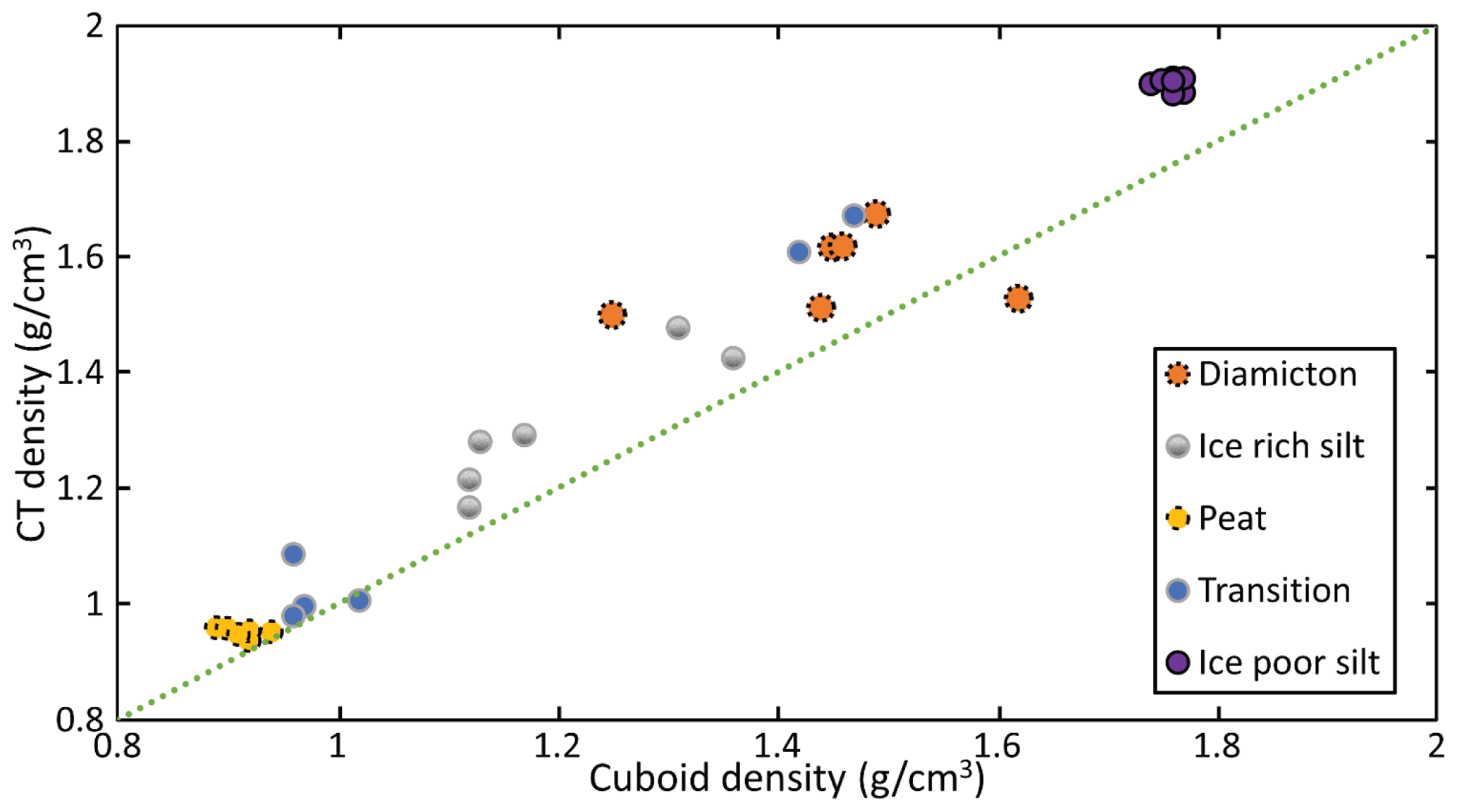
Figure 13 Estimated densities from CT image processing of 65 µm scans vs. calculated ones from the cuboid method.

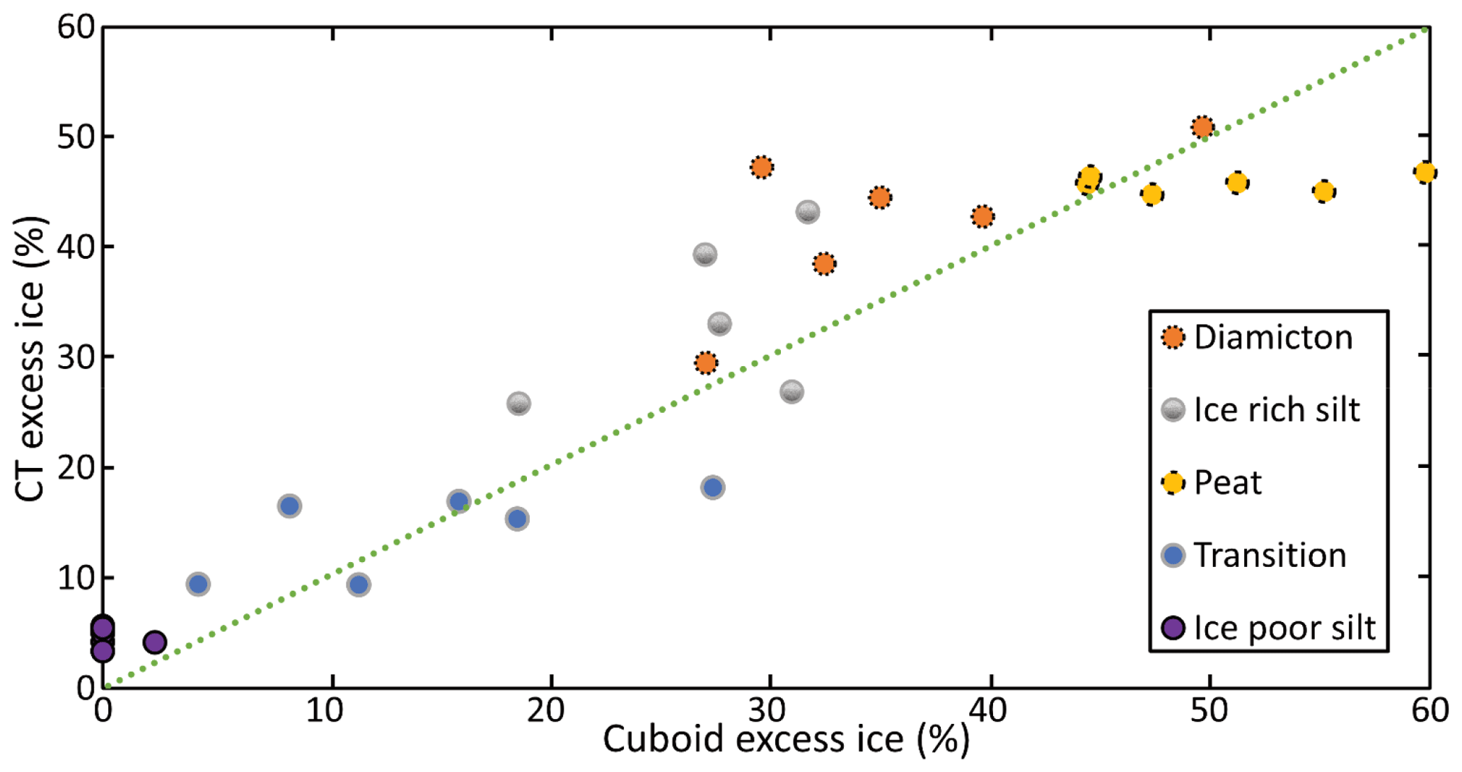
Figure 14 Estimated excess ice contents from CT image processing of 65 µm scans vs. calculated values from the cuboid method.

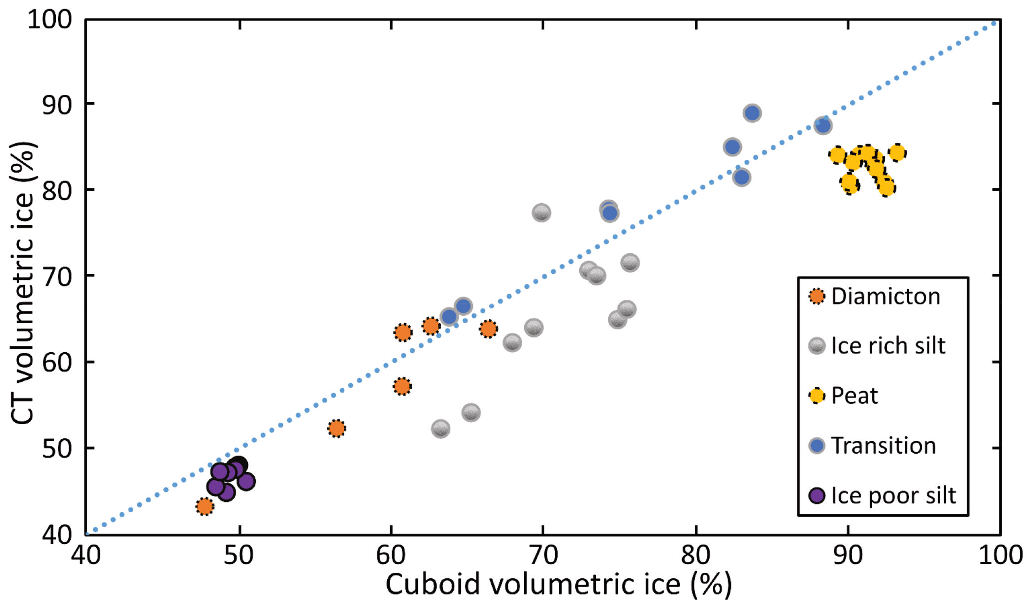
Figure 15 Estimated volumetric ice contents from CT image processing of 65 µm scans vs. calculated values from the cuboid method.

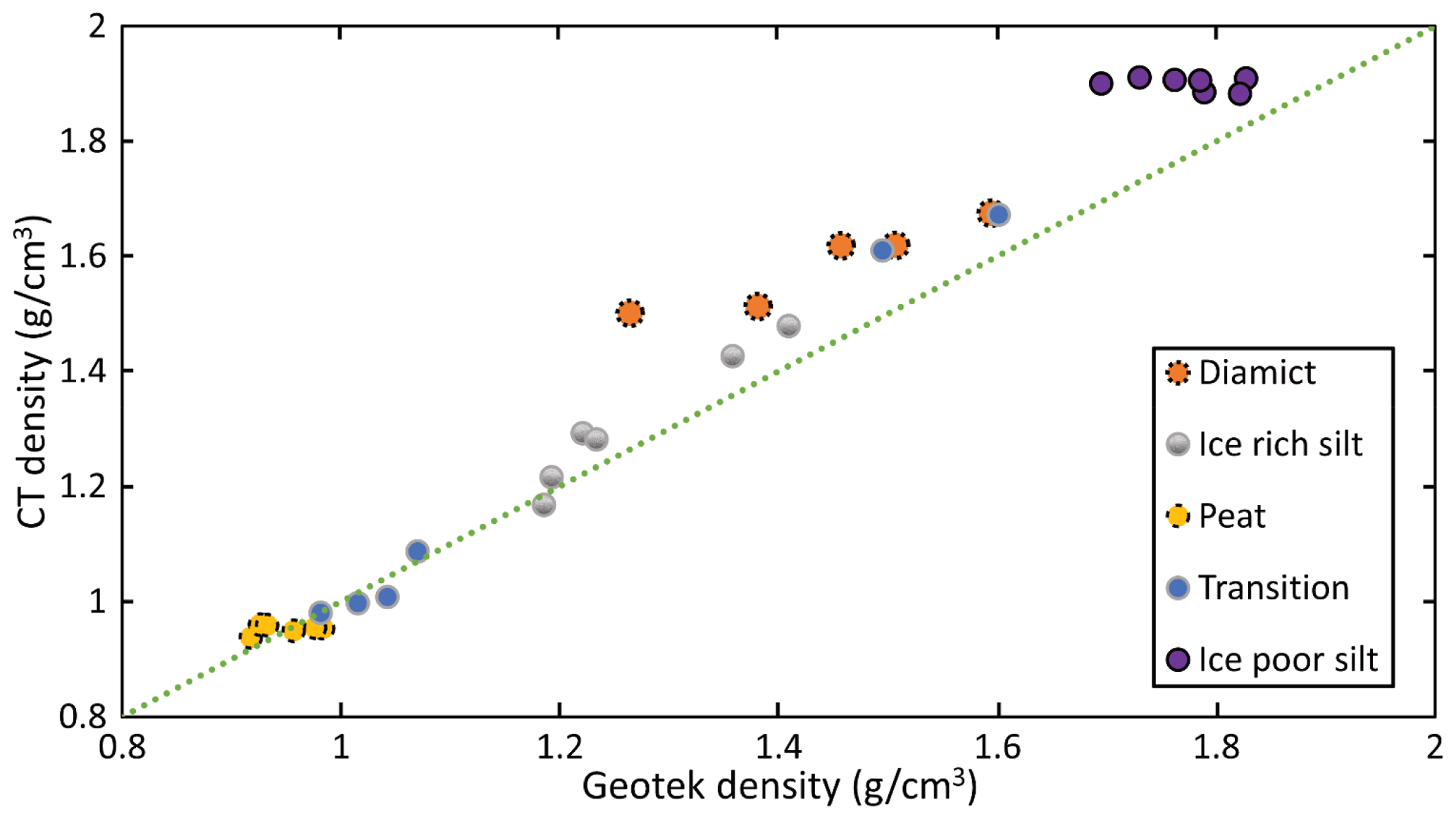
Figure 16 Estimated bulk density from CT image processing vs. calculated values from the MSCL method.

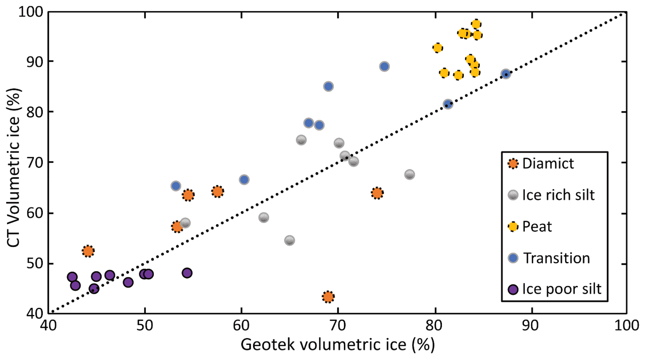
Figure 17 Estimated volumetric ice contents from CT image processing vs. calculated values from the MSCL method.

3.4 Comparison of non-destructive methods

The results of this study show strong agreement between the two non-destructive methods – CT and MSCL – and highlight the importance of the continued development and refinement of non-destructive methods for extracting physical properties from permafrost materials.

The presented CT method allows for whole-core high-resolution (65 µm) 3D imaging of cores, measurement of bulk density, and estimation of excess ice contents at a desired scale. This contrasts with MSCL which is restricted to a fixed data collection transect down the center of the core (∼ 1 cm wide) with a maximum sample resolution of ∼ 0.5 cm and high-resolution (25 µm) 2D half-core images and currently provides only volumetric ice estimates and no direct estimates of excess ice. The CT method is capable of estimating volumetric ice contents but requires cores to be subsampled to a smaller size (2 × 2 × 4 cm cube) to allow for finer-resolution scans (25 µm).

It is worth noting that the MSCL provides a more rapid method for collecting bulk density and volumetric ice content estimations in comparison with the CT method. However, in addition to bulk density and volumetric ice content estimations, the CT method can provide direct estimates of excess ice content. Visible ice can be segmented and isolated from the remaining sediment and pore ice when scanning split cores at 65 µm voxel size, allowing the opportunity to better estimate EIC values compared to MSCL methods. Therefore, in terms of a non-destructive method for identifying and quantifying excess ice within permafrost cores the CT method provides a more robust approach, although the image processing and acquisition costs are significantly greater.

4 Conclusions

This study investigated the application of high-resolution industrial CT scanning as a non-destructive method to tackle the limitations of traditional destructive methods (e.g., visual acuity, poor reproducibility, and low resolution) in permafrost characterization. Investigations were done by systematically logging permafrost cores, visualizing cryostructures, measuring bulk density, and estimating volumetric and excess ice contents independently. Five permafrost cores, representing common materials encountered in permafrost regions, were scanned at voxel sizes of 65 and 25 µm. A new calibration method was used to extract real densities in g cm⁻³ directly from CT images. Image segmentation results using the Otsu automatic image thresholding method illustrated the effectiveness of this method in generating robust segmentation results, while the visual inspection method has its own drawbacks, e.g. inspector's visual acuity and poor reproducibility.

The initial identification of different materials from CT images showed three classes – air (gas), ice, and sediments – while image processing steps of the scans (using the Otsu method) illustrated significant density differences in the ice and sediment classes. Image segmentation results using multiple image processing steps showed visual/excess ice as a lower density relative to the pore ice and delineated two sediment classes based on densities.

Since manual and visual thresholding is subject to operator experience and judgement and also not applicable in images with unimodal histograms related to materials with close densities (organic materials and ice), an automatic thresholding technique was used in this study to generate more consistent results.

A comparison of the image processing results and extracted physical properties of five permafrost cores was validated against a destructive method (cuboid) and MSCL non-destructive method. The results showed strong agreement between these three methods (CT and cuboid) considering their differing resolutions and regions of interest with overall average RMSEs of 3 %, 6 %, and 0.12 g cm⁻³ for VIC, EIC, and density, respectively. This agreement demonstrates the applicability and reliability of non-destructive methods in tracking physical and cryostructural details of permafrost cores and producing replicable, cost-effective measurements. A sensitivity analysis of the impact of differing resolutions on the delineation between ice and sediment showed that higher-resolution scans generate more accurate VICs, while the lower-resolution scans are still sufficient for the estimation of EICs and a rough estimation of VICs.

The proposed approach of this study will help build more robust permafrost datasets and strengthen future permafrost research efforts in mapping permafrost properties and the distribution of excess ice and predicting thaw settlement. It also presents an opportunity to develop methods to extract more information from existing datasets based on an acute understanding of the relations between key physical permafrost properties. The next steps can be followed by improving our understanding and techniques of scanning permafrost as well as using machine-learning-based image segmentation methods to generate datasets and explore the relations between physical permafrost properties.