Retrieval and validation of total seasonal liquid water amounts in the percolation zone of the Greenland ice sheet using L-band radiometry

Quantifying the total liquid water amounts (LWAs) in the Greenland ice sheet (GrIS) is critical for understanding GrIS firn processes, mass balance, and global sea level rise. Although satellite microwave observations are very sensitive to ice sheet melt and thus can provide a way of monitoring the ice sheet melt globally, estimating total LWA, especially the subsurface LWA, remains a challenge. Here, we present a microwave retrieval of LWA over Greenland using enhanced-resolution L-band brightness temperature (T_B) data products from the National Aeronautics and Space Administration (NASA) Soil Moisture Active Passive (SMAP) satellite for the 2015–2023 period. L-band signals receive emission contributions deep in the ice sheet and are sensitive to the liquid water content (LWC) in the firn column. Therefore, they can estimate the surface-to-subsurface LWA, unlike higher-frequency signals (e.g., 18 and 37 GHz bands), which are limited to the top few centimeters of the surface snow during the melt. We used vertically polarized T_B (V-pol T_B) with empirically derived thresholds to detect liquid water and identify distinct ice sheet zones. A forward model based on radiative transfer (RT) in the ice sheet was used to simulate T_B. The simulated T_B was then used in an inversion algorithm to estimate LWA. Finally, the retrievals were compared with the LWA obtained from two sources. The first source was a locally calibrated ice sheet energy and mass balance (EMB) model, and the second source was the Glacier Energy and Mass Balance (GEMB) model within NASA's Ice-sheet and Sea-level System Model (ISSM). Both models were forced by in situ measurements from six automatic weather stations (AWSs) of the Programme for Monitoring of the Greenland Ice Sheet (PROMICE) and the Greenland Climate Network (GC-Net) located in the percolation zone of the GrIS. The retrievals show generally good agreement with both the references, demonstrating the potential for advancing our understanding of ice sheet physical processes to better project Greenland's contribution to the global sea level rise in response to the warming climate.

1 Introduction

Continuous mass loss of the Greenland ice sheet (GrIS) has been a significant concern in the context of climate change and associated sea level rise (Khan et al., 2015; Mouginot et al., 2019; Otosaka et al., 2023; Shepherd et al., 2020). Greenland has lost about 330 billion tonnes of mass, equivalent to around 1 mm global sea level rise, per year on average for the last 2 decades (Greene et al., 2024; Khan et al., 2022). This will likely accelerate in the coming decades, even with the most optimistic warming scenario.

Mass loss occurs through surface melt and the subsequent runoff of meltwater towards the ice sheet margin and solid ice discharge (calving) at marine-terminating outlet glacier termini. While meltwater runoff has been the dominant contributor to mass loss in Greenland, both have increased in the last few decades (van den Broeke et al., 2016; Greene et al., 2024; Mouginot et al., 2019; Vandecrux et al., 2024a). In the ablation area, the winter snowpack is melted out every summer, and the meltwater enters an efficient drainage network of streams and lakes toward the margin (Smith et al., 2017). Higher up on the ice sheet, in the accumulation area, there is less melt, and a porous snow layer accumulated over the years, called firn, leads to the percolation and refreezing of surface melt, buffering additional sea level rise (Harper et al., 2012; Samimi et al., 2020). However, with intense and frequent melt events, thick ice layers, called ice slabs, are formed from meltwater refreezing, impeding vertical percolation of meltwater and promoting horizontal runoff (Culberg et al., 2021; Jullien et al., 2023; MacFerrin et al., 2019; Miller et al., 2022b, 2020b; Tedstone and Machguth, 2022). Increased refreezing resulted in a loss of approximately 5 % of GrIS firn air content (FAC) between 1996 and 2019 (Medley et al., 2022). These effects gradually diminish the ice sheet's inherent capability to retain meltwater and buffer sea level rise (Harper et al., 2012; Mikkelsen et al., 2016; Vandecrux et al., 2019).

Furthermore, increased melting contributes to forming supraglacial, englacial, and subglacial meltwater features (e.g., lakes, rivers, slush, crevasses, moulins, and firn aquifers) that can augment dynamical discharge and calving losses by lubricating the basal sliding surface and accelerating the flow of outlet glaciers (Hoffman et al., 2011; Schoof, 2010; Sundal et al., 2011; Zwally et al., 2002). Therefore, meltwater not only contributes to sea level rising through direct runoff, but it can also alter the physical structure that governs the dynamics and evolution of the ice sheet. Hence, quantification of total surface and subsurface liquid water is essential to understand ice sheet response to climate changes and project sea level rise accurately.

Surface melt and liquid water amount (LWA) can be estimated with various techniques. In situ AWS networks provide meteorological observations (Fausto et al., 2021), which can drive surface energy and mass balance (EMB) models to derive surface melt and LWA. Other in situ measurements, such as upward-looking radar (Heilig et al., 2018) or time domain resistivity probes (Samimi et al., 2021), can also be used to measure LWA at a given site. Due to logistical constraints, these point observations have a limited spatial and temporal coverage.

Regional climate models (RCMs) are primarily used to estimate ice-sheet-wide LWA, surface mass balance (SMB), and their changes (Fettweis et al., 2020). The results of RCMs are difficult to validate on the scale of the ice sheet, given the scarcity of in situ data to constrain and calibrate these models. Moreover, diversity exists in representation of the surface and subsurface firn processes among RCMs, leading to significant uncertainties in LWA estimates and their temporal and spatial variabilities (Fettweis et al., 2020; Thompson-Munson et al., 2023; Vandecrux et al., 2020; Verjans et al., 2019).

Satellite-based observations, especially microwave sensors, are very sensitive to ice sheet melting, manifested by large changes in dielectric constant with liquid water, and can provide global coverage in day–night and all-weather conditions (Abdalati and Steffen, 1997; Mote and Anderson, 1995; Picard et al., 2022; Tedesco, 2007; Tedesco et al., 2007; Zwally and Fiegles, 1994). Accordingly, both active (radars) and passive (radiometers) sensors have been used to monitor surface melting across Greenland and Antarctic ice sheets (Abdalati and Steffen, 1995, 2001; Hall et al., 2009; Mote, 2007; Nghiem et al., 2001; Tedesco, 2007; Wismann, 2000; Zwally and Fiegles, 1994). However, these conventional approaches applying high-frequency bands (i.e., 18 and 36 GHz) from the legacy and operational radiometers (Abdalati and Steffen, 1997; Ashcraft and Long, 2006; Colosio et al., 2021; Fettweis et al., 2007, 2011; Tedesco, 2007, 2009; Tedesco et al., 2007; Zwally and Fiegles, 1994) can only track the surface and near-surface binary melt status, not the meltwater propagation into the deeper layers, because of their limited penetration depth and sensitivity to LWC (Colliander et al., 2022a, b, 2023; Mousavi et al., 2022). The emergence of L-band (1–2 GHz) radiometry, marked by the launch of ESA's Soil Moisture and Ocean Salinity (SMOS) mission (November 2009–present) and the collaborative effort between NASA and Argentina's space agency CONAE in the Aquarius mission (October 2011–June 2015), followed by NASA's Soil Moisture Active Passive (SMAP) mission (March 2015–present), has opened up the possibilities for monitoring ice sheet meltwater at greater depths. L-band signals can penetrate deeper and provide a more accurate estimate of subsurface liquid water (Colliander et al., 2022a; Miller et al., 2020a, 2022a, b; Mousavi et al., 2022). Nevertheless, only a few attempts have been made to quantify the amount of liquid water (Colliander et al., 2022b; Houtz et al., 2019, 2021; Mousavi et al., 2021; Schwank and Naderpour, 2018).

Houtz et al. (2019) used the SMOS multi-angle L-band radiometric observations with a two-layer configuration of the L-band Specific Microwave Emission Model of Layered Snowpacks (LS-MEMLS) (Schwank et al., 2014) in an inversion-based retrieval framework for simultaneous estimation of snow liquid water content and density at the Swiss Camp site located in the ablation zone of the western Greenland ice sheet (GrIS). This initial study evaluated the results with in situ air temperature and another satellite-based empirical melt detection algorithm, called the XPGR (the cross-polarized gradient ratio of 19 and 37 GHz T_B) (Abdalati and Steffen, 1995, 1997); however, it did not include any in situ validation of actual LWA. Naderpour et al. (2021) supported the findings of Houtz et al. (2019) using close-range (CR) single-angle L-band microwave radiometer measurements and the same L-band specific forward model (LS-MEMLS) at the Swiss Camp location. Houtz et al. (2021) extended the Houtz et al. (2019) approach to estimate LWA over the entire GrIS, where they tuned the wet-layer thickness (10–100 cm) to provide variable estimates of LWA. Field observations and modeling results provide evidence of meltwater infiltration for more than 100 cm, especially in the percolation zone of the GrIS (e.g., Samimi et al., 2021; Vandecrux et al., 2020). Mousavi et al. (2021) developed an L-band specific snow/firn radiative transfer (RT) model to derive multidimensional brightness temperature look-up tables (LUTs) for the frozen and melt seasons considering a four-layer ice sheet structure. The algorithm uses frozen-season brightness temperature to determine the baseline emissions (temperature, density, scattering coefficient), which are then used in the melt season to estimate liquid water content and corresponding wet-layer thickness. None of these previous studies presented a validation approach for the LWA against any reliable reference. The primary motivation of this paper is to extend the approach of Mousavi et al. (2021) with improved and updated LUTs and to present a validation attempt for the LWA with two state-of-the-art surface energy balance models forced with in situ observations. We also provide the spatial and temporal variability in seasonal LWA over the percolation zone of the GrIS for 2015–2023.

2 Methods

2.1 SMAP L-band enhanced-resolution brightness temperatures

SMAP was launched on 31 January 2015 and has been operational since 31 March 2015 (Entekhabi et al., 2010). It was placed at a 685 km altitude, 98.1° inclination, sun-synchronous polar orbit with Equator crossings at 06:00 and 18:00 local time. It carries a conically scanning radiometer operating at 1.41 GHz (L-band) with a constant incidence angle of 40° that results in a 1000 km wide swath giving twice-daily coverage of the GrIS. It measures brightness temperature (T_B) in fully polarimetric mode, giving horizontal and vertical polarizations, and the third and fourth Stokes parameters with native 38 km spatial resolution. The radiometric precision of the SMAP radiometer is within 0.5 K (Chaubell et al., 2018, 2020; Piepmeier et al., 2017). For 20 June–23 July 2019 and 6 August–16 October 2022, SMAP does not have results because of an operational outage of the satellite.

Here, we used SMAP L-band enhanced-resolution T_B products generated using the radiometer form of the Scatterometer Image Reconstruction (rSIR) algorithm and projected on the EASE-2 3.125 km grid (Brodzik et al., 2021; Long et al., 2019). The rSIR algorithm leverages the measurement response function (MRF) of each observation and combines the overlapping MRFs to reconstruct enhanced-resolution T_B images. The effective resolution of SMAP enhanced-resolution T_B products posted on a 3.125 km grid is ∼ 30 km compared to the 46 km effective resolution of the SMAP original data products (Long et al., 2023). Therefore, it improves the overall effective resolution of about 30 % compared to coarser grid postings (Long et al., 2023; Zeiger et al., 2024). The data product provides two T_B images daily, in the morning and evening, facilitating the resolution of diurnal variability. The spatial oversampling and resolution enhancement enables an improved characterization of spatial heterogeneity (Long et al., 2023). The land–ocean mask used to locate the ice sheet edge comes from the Programme for Monitoring of the Greenland Ice Sheet (PROMICE) (Citterio and Ahlstrøm, 2013).

2.2 Microwave radiometric response of the GrIS

2.2.1 Theoretical background

Microwave radiometers measure the naturally emitted thermal radiation, called the brightness temperature (T_B), by the firn as observed in the microwave portion of the electromagnetic spectrum. It is related to the emissivity e and the effective physical temperature T_phy of snow/firn/ice media for a given frequency f, polarization p, and incidence angle θ. If firn were vertically homogeneous or isothermal, the T_B could be found according to Rayleigh–Jeans approximation (Ulaby and Long, 2014):

$$\begin{array}{}\text{(1)}& T_{\mathrm{B}}(f,p,\mathit{\theta })=e{T}_{\mathrm{phy}}.\end{array}$$

However, firn is not a vertically homogenous medium. Both the emissivity and temperature vary with depth. As a result, the T_B is given by a depth-integrated product of physical temperature and emissivity, weighted by the emissive, absorptive, and scattering properties of the snow/firn/ice layers (Jay Zwally, 1977), which is strongly dependent on the frequency of observation.

To account for the depth dependencies of snow and ice properties, firn is regarded as a complex multilayer dense medium. For each layer, an effective physical temperature and permittivity are determined from firn absorptive and scattering properties. Then, the microwave emission and its propagation are typically modeled using an equation of radiative transfer (RT). Considering firn to be a stack of N plane-parallel layers consisting of isotropic and homogeneous material in each layer, the RT equation can be given as (Jin, 1994, 1997; Picard et al., 2013; Tsang et al., 2000)

$$\begin{array}{}\text{(2)}& \begin{array}{rl}\cos \mathit{\theta }{\displaystyle \frac{\mathrm{d}}{\mathrm{d}z}}{\mathit{T}}_{\mathrm{B}}\left(z,\mathit{\theta },\mathrm{\varnothing }\right)& ={\mathit{\kappa }}_{\mathrm{a}}{T}_{\text{phy}}\left(z\right)\mathit{I}-{\mathit{\kappa }}_{\mathrm{e}}{\mathit{T}}_{\mathrm{B}}\left(z,\mathit{\theta },\mathrm{\varnothing }\right)\\ & +\underset{\mathrm{0}}{\overset{\frac{\mathit{\pi }}{\mathrm{2}}}{\int }}\underset{\mathrm{0}}{\overset{\mathrm{2}\mathit{\pi }}{\int }}\sin {\mathit{\theta }}^{\prime }\mathrm{d}{\mathit{\theta }}^{\prime }\mathrm{d}{\mathrm{\varnothing }}^{\prime }\mathbf{P}(\mathit{\theta },\mathrm{\varnothing },{\mathit{\theta }}^{\prime },{\mathrm{\varnothing }}^{\prime })\\ & \cdot {\mathit{T}}_{\mathrm{B}}\left(z,{\mathit{\theta }}^{\prime },{\mathrm{\varnothing }}^{\prime }\right).\end{array}\end{array}$$

Here, ${\mathit{T}}_{\mathrm{B}}\left(z,\mathit{\theta },\mathrm{\varnothing }\right)$ denotes the vertically and horizontally polarized brightness temperatures at depth z propagating along a direction characterized by θ (zenith angle) and ϕ (azimuth angle). κ_e, κ_a, and κ_s are the extinction, absorption, and scattering coefficients, respectively, representing medium properties. For an isotropic medium, the extinction coefficient can be described as ${\mathit{\kappa }}_{\mathrm{e}}={\mathit{\kappa }}_{\mathrm{a}}+{\mathit{\kappa }}_{\mathrm{s}}$. θ^′ and ϕ^′ are slant angles, and P is the bistatic scattering phase function. T_phy(z) is the physical temperature of snow at depth z, and I is a unit vector. Thus, the first term on the right-hand side of Eq. (2) represents the microwave emission (T_B) of snow/fir/ice from depth z, and the second term denotes the extinction (attenuation) of the emission due to absorption and scattering. The third term represents the sum of total scattered emission in the direction of the receiver (as specified by θ and ϕ). Equation (2) is solved analytically or numerically subject to boundary conditions at each layer interface and at the top and bottom of the medium.

The extinction coefficient, κ_e, is a function of the effective dielectric constant of the layer and frequency of the observation. Thus, the overall T_B is given by the depth-integrated profiles of the effective physical temperature and dielectric constant of each layer. Therefore, penetration depth plays a key role in determining the variability in T_B, especially in low-frequency bands. For a low-loss medium such as firn, the penetration depth can be approximated as (Elachi and Zyl, 2021)

$$\begin{array}{}\text{(3)}& \mathit{\delta }={\displaystyle \frac{c\sqrt{{\mathit{\epsilon }}^{\prime }}}{\mathrm{2}\mathit{\pi }f{\mathit{\epsilon }}^{\prime \prime }}},\end{array}$$

where c is the speed of light and ε^′ and ε^′′ are the real and imaginary parts of the dielectric constant of the firn. As shown, δ is inversely proportional to both f and ε^′′. The L-band signal thus penetrates a significantly thicker layer than the higher frequency, such as the Ka-band signal. Liquid water markedly increases ε^′′ (compared to $\sqrt{{\mathit{\epsilon }}^{\prime }}$ in proportion), decreasing the penetration depth for any frequency. For a typical snow density (measured for dry snow) in the percolation zone, it can be more than 4 m for an average LWC of less than 1 % with the Ulaby and Long (2014) model's wet snow dielectric constant, decreasing exponentially with the LWC. Thus, for an average LWC of 3 % and higher, it is around 1 m and less. The average LWC in the percolation zone is typically not higher than 4 %, except for extraordinary melt years (such as 2012, not included in the study), and typical infiltration of liquid water is also generally within the upper 4 m (Samimi et al., 2020, 2021).

There are two types of scattering processes in the snow/firn medium affecting the propagation: surface scattering and volume scattering. The relative size of the scatterers compared to the wavelength determines the degree and types of scattering. For high-frequency bands (> 10 GHz), the impact of volume scattering is critical because the fractional volume of scatterers (snow/firn) is significant. This is why the high-frequency signals interact more with fresh snow, grain size, and roughness at the surface. Low-frequency signals (<10 GHz) are relatively insensitive to volume scattering from snow grains because the size of the scatterers is much smaller than the wavelength. Surface scattering occurs due to surface irregularities at the interface between layers of different dielectric constants, affecting all the frequencies when present. Horizontal and vertical ice layers (strata) are formed at various depths in the firn primarily from the refreezing of seasonal snowmelt. Over time, older ice layers move downward due to the snow accumulation, while new ice layers are formed for subsequent melts at the top layers, creating a complex set of stratigraphy and significantly influencing the L-band signals from the deeper layers. Therefore, L-band T_B is determined by the subsurface temperature, stratigraphy, and LWA.

2.2.2 Frozen-season response

L-band T_B exhibits some distinct spatial features over the GrIS during a frozen season. Along a typical west–east transect, T_B is the highest in the ablation zone, then it gradually decreases to its lowest value in the percolation zone, followed by a gradual increase towards a moderate value in the upper accumulation zone. A mirror image is seen on the eastern side of the ice sheet. The spatial features of H-pol T_B are similar to V-pol T_B, but they are more affected by subsurface layering. This is illustrated in Fig. 1 with V- and H-pol mean frozen-season T_B values and their normalized polarization ratio (NPR; defined as NPR = (TBV − TBH) $/$ (TBV + TBH)). The ablation zone is characterized by exposed glacial ice with a higher density and internal temperature than the ice sheet towards Greenland's interior. It is soaked and swept by a large amount of meltwater every year. During the frozen season, the L-band emission has a high effective emissivity, radiating the warmer physical temperature of the deeper layers. In the percolation zone, on the other hand, moderate but varying melt occurs almost each year or every few years and percolates down and refreezes at different depths, forming discrete ice layers and ice pipes and causing substantial scattering of mean T_B (Jezek et al., 2018). High NPR values highlight the area with dense ice layers (strata). The upper accumulation zone experiences light or no melt but accumulates snow, resulting in less density variation compared to the percolation zone. For detecting melt and quantifying LWA, we used vertically polarized T_B (V-pol T_B) considering its lower sensitivity to subsurface stratigraphy.

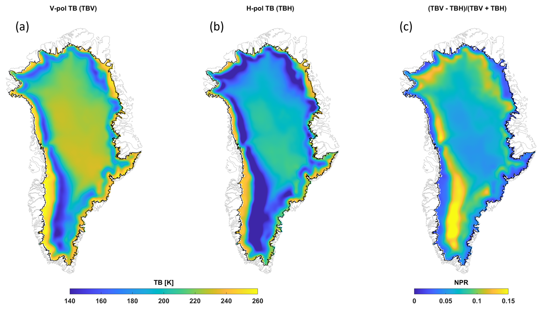
Figure 1 L-band radiometric response of the GrIS during the frozen season. Vertically polarized T_B (a) and horizontally polarized T_B (b) averaged over 1 January–7 April 2015–2023 and their normalized polarization difference (c).

2.2.3 Melt-season response

During the summer season in presence of melt, the L-band T_B generally decreases in the ablation and upper accumulation zones compared to the frozen season, while it increases significantly in the percolation zone. Figure 2 illustrates this for a sample summer day (31 July 2019) when melt was detected across the K transect (∼67° constant latitude; see the red line in Fig. 2a). The melt flags (square symbols over the dashed line) specify the T_B samples for which melt was detected (Sect. 3.2). The presence of LWC in the snow and firn increases the absorption and emission in turn (Mote and Anderson, 1995). However, at the lower elevation around the ablation zone, the T_B decreases from its very high level (∼260 K) as the LWC of the seasonal snow layer increases. This is because, when the LWC in the snow layer exceeds a threshold, snow becomes saturated and creates a reflective boundary at the ice and snow interface, suppressing the emission from the ice layer and resulting in overall lower T_B. This is caused by intense melting common in the ablation zone (Fig. 2b). The percolation zone experiences moderate melt, making the snow and firn highly absorptive during melt season. As a result, the T_B gradually increases from its winter references (Fig. 2b), making the L-band sensitive to the total amounts of melt. In the upper accumulation zone, melt seldom occurs. However when it does occur, it may percolate and refreeze quickly in the colder snow, creating ice layers that cause reflection and reducing L-band T_B signals.

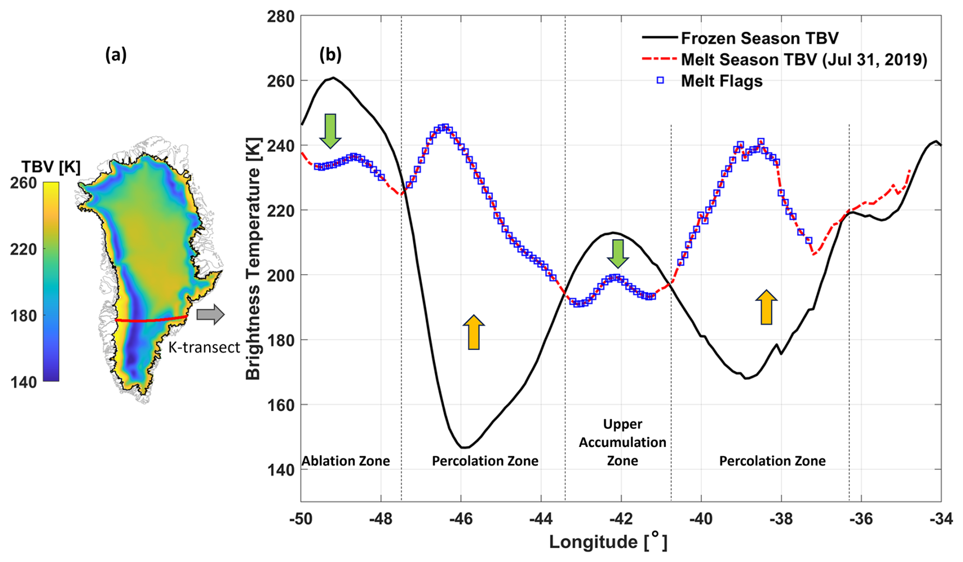
Figure 2 Radiometric response of L-band T_B during the frozen season and melt season. The location of the K transect is highlighted by the red line over the mean frozen-season TBV map (a). Corresponding T_B values across the transect are shown in pane; (b): the black line represents the mean V-pol T_B during the frozen season (1 January–7 April of the same year). The red dash-dotted line indicates T_B responses on a sample melt day (31 July 2019). The blue square symbols on the red dash-dotted line depict melt flags (melt detections). The approximate locations of ablation, percolation, and upper accumulation zones are depicted along the K transect for reference.

Figure 3 shows the L-band V-pol T_B time series during March–October 2016 at the DY2 AWS, a location representative of the percolation zone. During the frozen season, the L-band T_B is relatively lower and stable. During the melt season, it captures the diurnal signals during melting phases (melt generation). However, it diminishes as the melt percolates to deeper layers. From the onset through the end of the melt season, the density and grain size increase in the snow and firn layers due to melt (Vandecrux et al., 2022). Although the L-band T_B is relatively insensitive to the grain growth, the post-melt T_B level may still decrease because of increased reflection from newly formed ice layers. This effect is pervasive, especially across the accumulation zone, justifying a dynamic threshold in threshold-based melt detection algorithms.

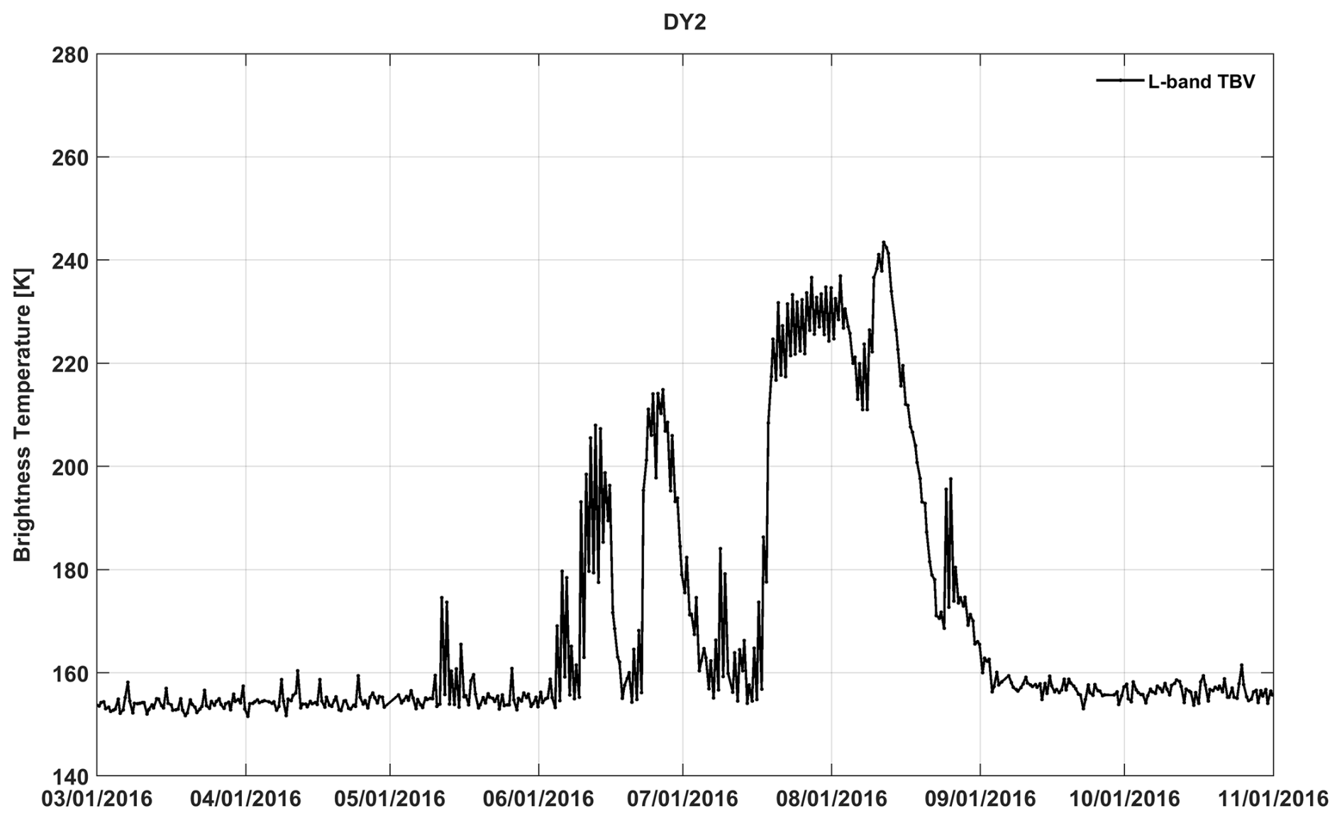
Figure 3 L-band V-pol T_B time series at the DY2 automatic weather station location (66.482453° N, 46.294145° W) during March–October 2016, illustrating the change in T_B level caused by melting, snow accumulation, and other physical processes.

2.3 Melt retrieval algorithm

We used a threshold-based empirical detection algorithm to detect surface and subsurface melt events. The threshold is determined by

$$\begin{array}{}\text{(4)}& T=\mathit{\mu }\pm m\mathit{\sigma },\end{array}$$

where μ is a reference T_B (the mean during the frozen season), σ is the standard deviation of the T_B during the reference period, and m is an empirically derived constant. A constant value of 10 was chosen for m. Firstly, to detect the first and last melt during 1 year for a grid point, the mean T_B values during 1 January–7 April and 24 October–31 December, respectively, were used as the reference values. The period of 1 January–31 March is generally considered to have fully frozen conditions regardless of elevation and latitudes. SMAP does not have data for 1 January–30 March 2015 because the data production started on 31 March 2015; therefore, we extended the reference period to 7 April for all the years to make our data consistent. The period of 24 October–31 December was determined based on visual observations of the time series during 2015–2023. An averaged value of σ_spring and σ_fall is used with a final adjustment of m in such a way that the threshold does not miss the first and last melts. Then, a linearly transitional reference value is used between the first and last melt days to account for the change in T_B for subsequent melt because of refreezing.

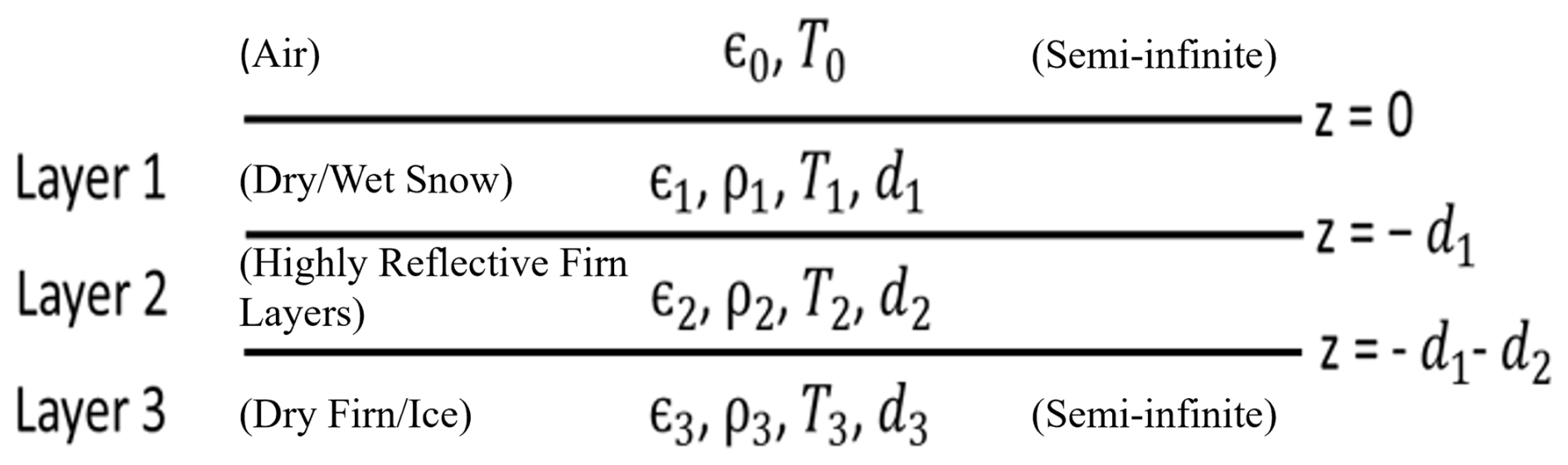
We used an inversion of a simplified ice sheet emission model to estimate the LWA and physical properties of the detected melt events. The retrieval algorithm consists of a forward model (Fig. 4) simulating the L-band T_B (Mousavi et al., 2021) and a cost function minimization between the simulated and observed T_B. The forward model represents the ice sheet as a stack of four vertical layers, where each layer is characterized by its complex dielectric constant (ε), density (ρ), physical temperature (T), and thickness (d). The top layer is air above the snow and is assumed to be semi-infinite (surface to radiometer antenna), and the bottom layer (Layer 3 in Fig. 4) is also assumed semi-infinite, while the intermediate layers are configured with variable thicknesses. The first snow/firn layer (Layer 1 in Fig. 4) holds dry and wet snow/firn during frozen and melt seasons, respectively. To account for the combined reflective effects by the complex stratigraphy due to numerous ice layers common in the percolation zone of the GrIS, along with the effects of multiple scattering in the snow/firn layer, we designate Layer 2 (underneath the dry/wet snow/firn layer) as a highly reflective layer by explicitly specifying its dielectric constant (with a high real part that varies spatially). The T_B is then modeled using the incoherent approach of radiative transfer (RT) theory, without considering the effects of volume scattering analytically (but considering its dielectric effects explicitly). For a specific depth z, the upwelling T_B for a given polarization, p, is given by

$$\begin{array}{}\text{(5)}& \begin{array}{rl}{T}_{\mathrm{B}n\mathrm{p}}^{\mathrm{u}}\left({\mathit{\theta }}_n,z\right)& =\left[{\mathrm{\Gamma }}_{n\mathrm{p}}{T}_{\mathrm{B}n\mathrm{p}}^{\mathrm{d}}\left({\mathit{\theta }}_n,-d_n\right)+\left(\mathrm{1}-{\mathrm{\Gamma }}_{n\mathrm{p}}\right)\right.\\ & \left.\cdot T_{\mathrm{B}\left(n+\mathrm{1}\right)p}^{\mathrm{u}}\left({\mathit{\theta }}_{\left(n+\mathrm{1}\right)},-d_n\right)\right]e^{-k_{\mathrm{a}n}(z+d_n)\text{sec}{\mathit{\theta }}_n}\\ & +(\mathrm{1}-e^{-k_{\mathrm{a}n}(z+d_n)\text{sec}{\mathit{\theta }}_n})T_n,\end{array}\end{array}$$

where $T_{\mathrm{B}n\mathrm{p}}^{\mathrm{u}}$ and $T_{\mathrm{B}n\mathrm{p}}^{\mathrm{d}}$ represent the upwelling and downwelling p-polarized T_B at the interface $z=-d_n$ characterized by reflectivity Γ_np. θ_n is the incidence angle determined from the Snell's law and dielectric constant, and k_an is the power absorption coefficient given by $k_{\mathrm{a}n}=-\mathrm{2}Re\mathit{\left\{}\mathit{\omega }\sqrt{{\mathit{\epsilon }}_n{\mathit{\mu }}_{\mathrm{0}}}\mathit{\right\}}$, where ω is the angular frequency, ε_n is the complex permittivity of the layer, and μ₀ is the magnetic permeability for a nonmagnetic material. T_n is the physical temperature of the layer and assumed to be homogenous within the layer. The downwelling part of the T_B, $T_{\mathrm{B}n\mathrm{p}}^{\mathrm{d}}\left({\mathit{\theta }}_n,-d_n\right)$, is given by

$$\begin{array}{}\text{(6)}& \begin{array}{rl}{T}_{\mathrm{B}n\mathrm{p}}^{\mathrm{d}}\left({\mathit{\theta }}_n,-d_n\right)& ={\mathrm{\Gamma }}_{(n-\mathrm{1})p}{T}_{\mathrm{B}n\mathrm{p}}^{\mathrm{u}}\left({\mathit{\theta }}_n,-d_{n-\mathrm{1}}\right)\\ & +(\mathrm{1}-{\mathrm{\Gamma }}_{(n-\mathrm{1})p})T_{\mathrm{B}(n-\mathrm{1})\mathrm{p}}^{\mathrm{d}}\left({\mathit{\theta }}_{(n-\mathrm{1})},-d_{n-\mathrm{1}}\right).\end{array}\end{array}$$

It is assumed that there are no downward and upward emissions beyond the top and bottom semi-infinite layers, respectively, and that the atmospheric attenuation is also negligible considering L-band frequency. Therefore, the top of the atmosphere T_B is found from Eq. (1),

$$\begin{array}{}\text{(7)}& T_{\mathrm{BP}}\left({\mathit{\theta }}_{\mathrm{0}},H\right)\approx T_{\mathrm{B}\mathrm{0}\mathrm{p}}^{\mathrm{u}}\left({\mathit{\theta }}_{\mathrm{0}},\mathrm{0}\right)=(\mathrm{1}-{\mathrm{\Gamma }}_{\mathrm{0}\mathrm{p}})T_{\mathrm{B}\mathrm{1}\mathrm{p}}^{\mathrm{u}}\left({\mathit{\theta }}_{\mathrm{1}},\mathrm{0}\right).\end{array}$$

Figure 4 L-band multilayer ice sheet forward model.

For faster processing during retrieval, we developed separate look-up tables (LUTs) for dry and melt season, prescribing layer parameters by sweeping over a realistic range of each parameter. The main difference in the LUTs, compared to the LUTs in Mousavi et al. (2021), is in the range of the background temperature. Mousavi et al. (2021) used a lower range for background temperature (110–265 K) for the highly reflective layer (Layer 2 in Fig. 4) and the semi-infinite ice layer (Layer 3 in Fig. 4) in generating the LUTs, originally developed for modeling the Antarctic ice sheet (Mousavi et al., 2022). We constrained it between 200 and 273.15 K, as appropriate for the GrIS. The changes in the range of the other background parameters are minor, except the resolutions. For each layer, dry snow density varied from a fresh snow density of 50 kg m⁻³ to that of solid ice of 917 kg m⁻³. For the melt season, the wet snow layer is inserted with a volume fraction of meltwater, m_v, which is varied from 0 % to 5 % in 40 equally spaced steps, and thickness, d_wet, which is varied from 10 cm to 20 m in 10 cm steps for the top 60 cm, in 20 cm steps for next 1.4 m, in 40 cm steps for next 8 m, and in 1 m steps for the next 10 m. For m_v>0, T_wet must be 0 °C. Colbeck (1974) suggested that, because of capillary retention, the irreducible water saturation of dense snow/firn is about 7 % of its pore volume. Coléou and Lesaffre (1998) showed that the irreducible water content can be up to 6.5 %–8.5 % of the pore volume depending on the density. Based on these studies and considering snow/firn density in the percolation zone, we determined the maximum volume fraction to be 5 %. The dielectric constant of the dry snow was calculated using Mätzler (2006), and that of wet snow was calculated following Ulaby and Long (2014). The Ulaby and Long (2014) model of wet snow dielectric constant is an empirical model, called the “modified Debye-like model”, which is an extension of Hallikainen et al. (1986). Then, the emission model was run for each combination. The model computes the top-of-the-atmosphere L-band T_B at the V- and H-pol assuming a fully transparent atmosphere. With all these constraints, the tuning finally results in two LUTs with six and eight dimensions for the dry and melt seasons, respectively.

The inversion was performed by optimizing a cost function that minimizes the distance between the LUT-modeled T_B and the corresponding SMAP-measured T_B for each 3.125 km grid cell. The optimization was carried out in two steps for each melting grid. Firstly, the frozen-season snow/firn density, physical temperature, and dielectric constant were estimated. Secondly, using that information, the volume fraction of meltwater m_v and corresponding wet-layer thickness d_wet were determined for a time stamp during the melt season. The LWA is thus the product of the two; i.e., LWA=m_vd_wet [m] m.w.e. This represents the instantaneous total LWA present in the SMAP footprint for that time stamp within the SMAP sensing depth, covering the typical infiltration of the meltwater in the percolation zone as per the climatological records (Samimi et al., 2020; Vandecrux et al., 2020). The detection algorithm uses both increasing and decreasing summer T_B values (w.r.t. threshold T from Eq. 4) to generate melt flags; however, the inversion only considered increasing T_B for LWA quantification. We averaged twice-daily LWA outputs to compute daily samples.

2.4 Automatic weather station measurements

Direct measurements of LWA are not available for validation. However, AWS networks, such as the Greenland Climate Network (GC-Net) (Steffen et al., 1996; Steffen and Box, 2001) or the Programme for Monitoring of the Greenland Ice Sheet (PROMICE) (Fausto et al., 2021), provide essential surface parameters that can be used to estimate LWA with an energy balance model. The Geological Survey of Denmark and Greenland (GEUS) now manages these two AWS networks, which cumulate 33 active ice sheet sites in Greenland that provide a suite of measurements, such as incoming/outgoing short and longwave radiation fluxes, snow surface height, air temperature, air pressure, vector winds, and subsurface temperature and density profiles (Fausto et al., 2021).

We used the hourly measurements from six PROMICE and GC-Net AWSs in the percolation zone to force an EMB model that produces a reference LWA, which was then used to validate the LWA retrieved from SMAP observations. The stations were selected considering their locations (see Fig. 5) and melt climatology. The meteorological forcing governs the surface energy budget (SEB) and was used to derive a coupled energy balance and a snow/firn hydrology model (Ebrahimi and Marshall, 2016; Samimi et al., 2021) that provide an estimate of hourly LWC evolution within snow and firn.

2.5 Ice sheet energy balance and hydrology model

The energy balance model (EBM) determines the net energy available for melting by considering the SEB along with modeled surface temperature, thermal emissivity, and albedo. The coupled model also accounts for the hydrological processes like meltwater infiltration, refreezing, and retention within the firn. We used two ice sheet EBMs for comparisons with the SMAP LWA retrievals. A detailed description of these models is beyond the scope of this article, but brief descriptions are given below. Readers are referred to relevant cited articles for further details.

2.5.1 Energy balance and hydrology model

A locally calibrated and validated EBM (Ebrahimi and Marshall, 2016; Samimi et al., 2020, 2021) was used as the primary reference for comparison. The EBM was initialized with ice core density profiles, stratigraphy, and subsurface temperature profiles (Vandecrux et al., 2023) and was forced with the hourly surface forcing from PROMICE and GC-Net AWSs. The model first calculates the net energy balance from the surface forcing by combining the energy fluxes towards the surface layer. Then, it runs a subsurface model to calculate heat conduction and melt rates in the upper 20 m of the snow/firn by resolving the profile into 43 vertical layers, with gradually decreasing thickness near the surface.

When the surface temperature reaches the melting point and the net energy is positive, melting occurs. Conversely, if net energy is negative and the surface layer is at the melting point, any existing liquid water will freeze, releasing latent heat and causing the surface layer to cool until all liquid water is refrozen, depending on the energy balance. When surface layer temperatures are below the melting point, and there is either an excess or deficit of energy leading to warming or cooling, the energy balance within a one-dimensional model of subsurface temperature evolution determines the subsurface temperature and density profiles. The model determines hydraulic conductivity and permeability after Meyer and Hewitt (2017), while thermal conductivity was modeled following Calonne et al. (2019). The profile then governs the availability of local water at any level for the next time stamp. The model relates to a basic approach to how meltwater flux percolates downward using Darcy's law. The local water balance is determined by mass conservation in each subsurface layer. Once a layer becomes temperate, it can retain liquid water within its pore space or allow it to percolate deeper (Coléou and Lesaffre, 1998). The subsurface model is coupled with a hydrology model that redistributes the meltwater; depending on the subsurface temperature profile, the meltwater may refreeze. Due to refreezing, density may increase, and ice layers may form that may reduce or completely block meltwater infiltration. The firn densification was modeled as in Vionnet et al. (2012). We henceforth refer to this model as the EBM for simplicity. To evaluate the LWA retrieval, we calculate the daily average LWA from the hourly EBM output.

2.5.2 Glacier Energy and Mass Balance (GEMB) model

We used output from GEMBv1.0 as a secondary source of comparison. It is a module in the Ice-sheet and Sea-level System Model (ISSM; https://issm.jpl.nasa.gov/, last access: 20 September 2024) that models the ice sheet surface energy and mass exchange and snow/firn state in a one-dimensional column over time (Gardner et al., 2023). It has more than 100 vertical layers with <5 cm thickness in the top layers and employs spatially variable grid size based on the ice sheet dynamics. GEMB formulates irreducible water content according to Colbeck (1973) and uses a bucket scheme (Steger et al., 2017) for liquid water infiltration. Parameterization of firn densification and thermal conductivity follows Herron and Langway (1980) and Sturm et al. (1997), respectively. Readers are referred to Gardner et al. (2023) and references therein for further details. The model was forced with the same hourly surface forcing from PROMICE and GC-Net AWS, but gap filled with ERA5 (Hersbach et al., 2020) atmosphere and radiation conditions, after the methods described by Paolo et al. (2023). The ERA5 surface temperature and downwelling longwave radiation forcing were spatially bias-corrected for each month, such that all values were adjusted by the difference between the RACMO2.3 (Noël et al., 2016) and the ERA5 1980–2015 monthly means. GEMB outputs include temperature, density, and LWC profiles.

2.5.3 Evaluation metrics

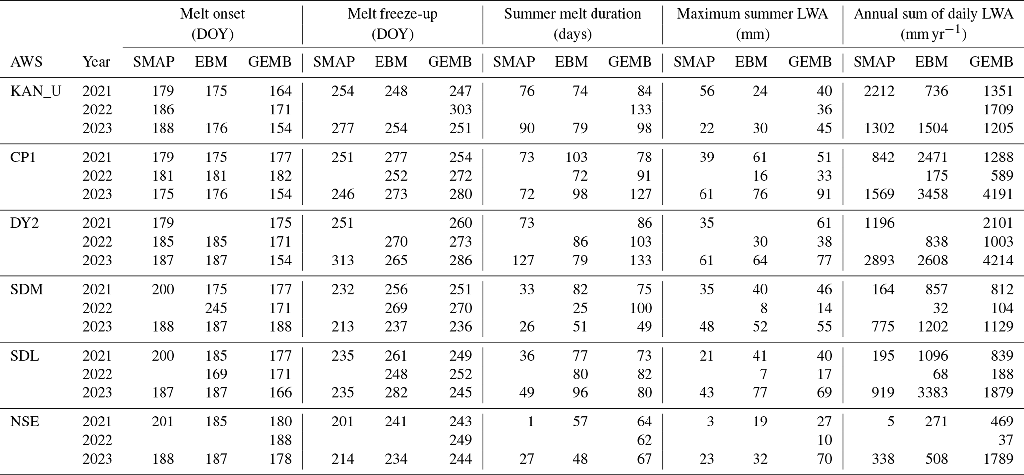
To compare SMAP daily LWA time series with corresponding LWA from the EBM and GEMB models, we considered the standard evaluation metrics, including mean difference, standard deviation (SD), mean absolute difference (MAD), Pearson linear correlation coefficient (r), and root-mean-square error (RMSE), for summer seasons (1 June–31 October 2021–2023). We also compared the day of melt onset (the first day of summer melt) and melt freeze-up (the last day of summer melt), the summer melt duration (difference of melt onset and freeze-up), the maximum summer LWA, and the annual sum of daily LWA (LWA_YS). To determine the day of melt onset and freeze-up, we only considered melt events with LWA >2 mm, to avoid any spurious melts that may result from any instrumental noise or other sources. The LWA_YS is the sum of daily LWA over 1 year. It is a measure of the total seasonal LWA, but it does not represent the total surface melt generated over 1 year. This is because SMAP observes the instantaneous LWA, the net water balance, which is the cumulative sum of surface melt, refreezing, and runoff over SMAP footprint. When the net water balance remains positive overnight, it can be considered multiple times in the total integrated LWA as long as it persists.

3 Results

3.1 Liquid water amount

3.1.1 Comparison to locally calibrated EBM

Figure 5 shows a comparison of the SMAP-retrieved LWA with the LWA derived from the EBM at six different PROMICE and GC-Net AWS sites for the 2023 summer season (1 June–31 October). The melt season at the CP1 site (Fig. 5a) began in the fourth week of June, according to both SMAP and the EBM, and continued through the first week of September according to SMAP, while it extended through the end of September in the model estimate. Shortly after the complete refreezing of the first melt event in late June, SMAP resumed recording LWA in the first week of July. Both SMAP and the EBM closely agree in both phase and magnitude of LWA during first half of July. Afterwards, the EBM reports overall higher LWA for the rest of the season, and it seemed to retain liquid water for an elongated period when SMAP showed a fully refrozen firn. The overall agreement is given by the Pearson linear correlation coefficient (r) of 0.79 and root-mean-square difference (RMSD) of 19 mm. The onset of the melt event at the KAN_U site (Fig. 5b) is concurrent to CP1 in accordance with the EBM. However, SMAP did not record melting at this site until the first week of July. Unlike the CP1 site, SMAP reports persistent LWA through the first week of October, whereas EBM shows complete refreezing by the second week of September. Both SMAP and the EBM captured a smaller LWA at the KAN_U site compared to the CP1 site. This is somewhat counter-intuitive because the KAN_U site is located at a lower elevation than the CP1 site (see the elevation in Fig. 5d). In fact, KAN_U is characterized by having a lower accumulation and higher melt rate every year (MacFerrin et al., 2019; Machguth et al., 2016). However, excessive melt has also created thick ice slabs in this location (MacFerrin et al., 2019; Machguth et al., 2016). As a result, liquid water cannot percolate to the deeper layers and run off horizontally. The model excludes this liquid water in the form of “drainage”, and SMAP only sees the existing meltwater in its field of view. At the DY2 site (Fig. 5c), LWA estimated by SMAP and the EBM are more closely resembled both in phase and magnitude (except the difference in timing of complete freeze-up). This is reflected by a nearly perfect correlation (r=0.98) and a small overall RMSD (4 mm) as shown.

SMAP LWA also closely aligns with the EBM at the NSE site in magnitude and duration of liquid water presence (r=0.98 and RMSD = 3 mm), although SMAP seemed to miss the late August small melt event (Fig. 5e). The agreement, however, exhibits the greatest deficiencies at the SDL site for this melt season (Fig. 5f). Although the timing of the melt onset and late August secondary melt event matches precisely, the EBM reports an overall higher LWA and an extended summer melt duration at this location. This is manifested in the performance metrics shown by a relatively higher RMSD (24 mm) and comparatively lower correlation coefficient (0.77). The performance at the SDM site is generally good (r=0.92 and RMSD = 6 mm), except the EBM demonstrates a delayed refreezing compared to SMAP (Fig. 5g).

It is pertinent to highlight that, while in situ LWAs at all these AWSs were derived from the energy balance model forced by the pointwise measurements at the AWS locations, the SMAP retrievals estimated a spatially averaged LWA corresponding to the ∼30 km effective resolution of the enhanced-resolution T_B. Approximately during the first half of the melt season, the LWA is primarily determined by meltwater generation in response to the net radiation flux at the surface, whereas, roughly during the second half, when the net radiation flux remains negative, refreezing becomes the dominant process. Hence, the model's representation of the surface melt infiltration, heat transfer, and other physical processes plays a significant role, posing additional uncertainties. The AWS measurements used to run the model also add some inherent uncertainties. Therefore, assessing relative accuracy is not straightforward. Nevertheless, the general agreements between the model- and SMAP-retrieved LWA in magnitude and phase at these locations suggest that the spatial heterogeneity of melt processes is not acute in these areas.

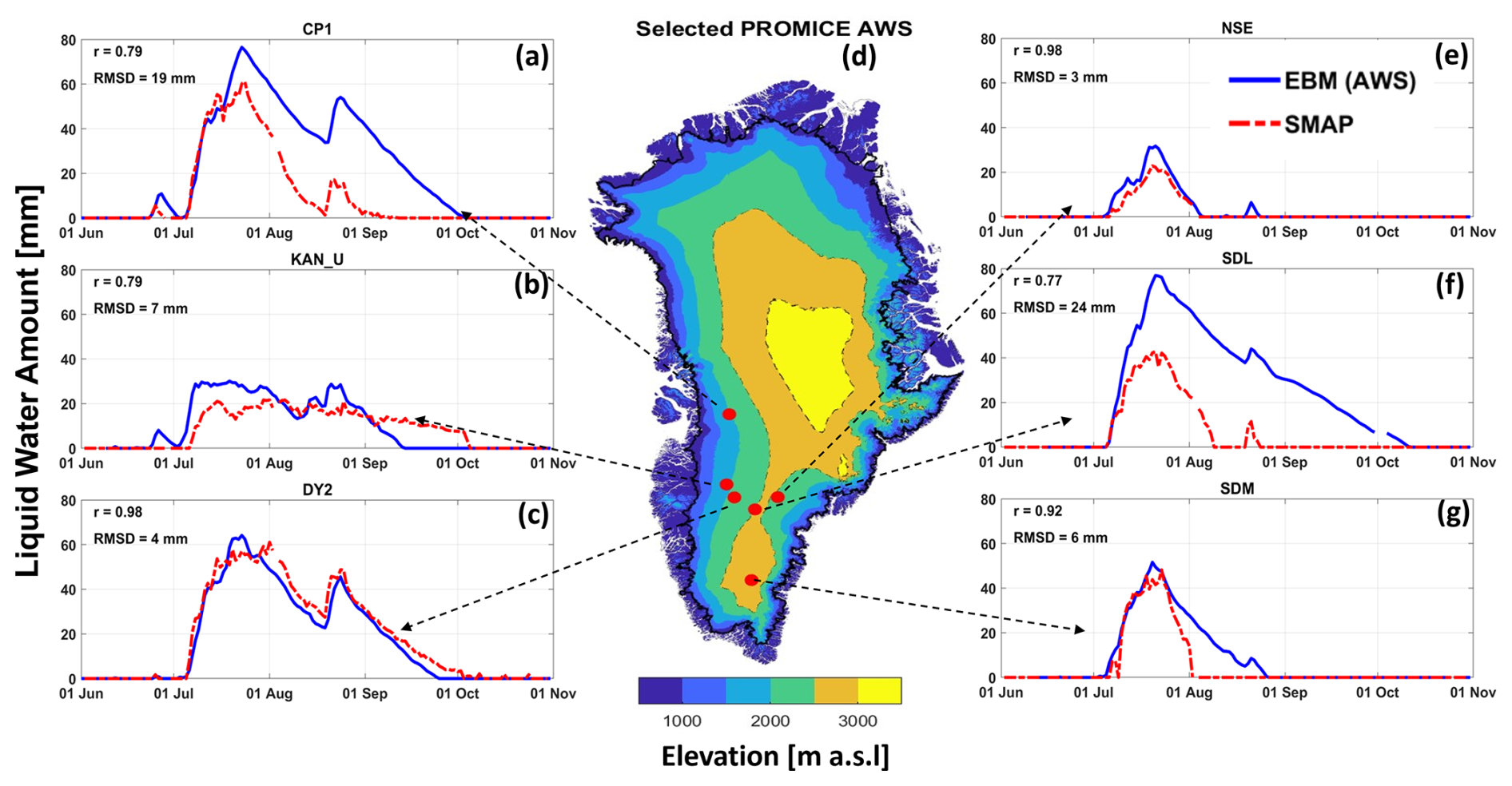
Figure 5 Comparison of the total daily liquid water amount retrieved from SMAP (dashed red lines labeled SMAP) and estimated by the EBM forced with in situ measurements (blue lines labeled EBM) at selected PROMICE and GC-Net AWSs within the GrIS percolation area for 1 June–31 October 2023. The locations of the AWSs are shown in the middle panel along with the ice sheet surface elevation (Howat et al., 2014).

3.1.2 Three-way comparison: SMAP, EBM, and GEMB model

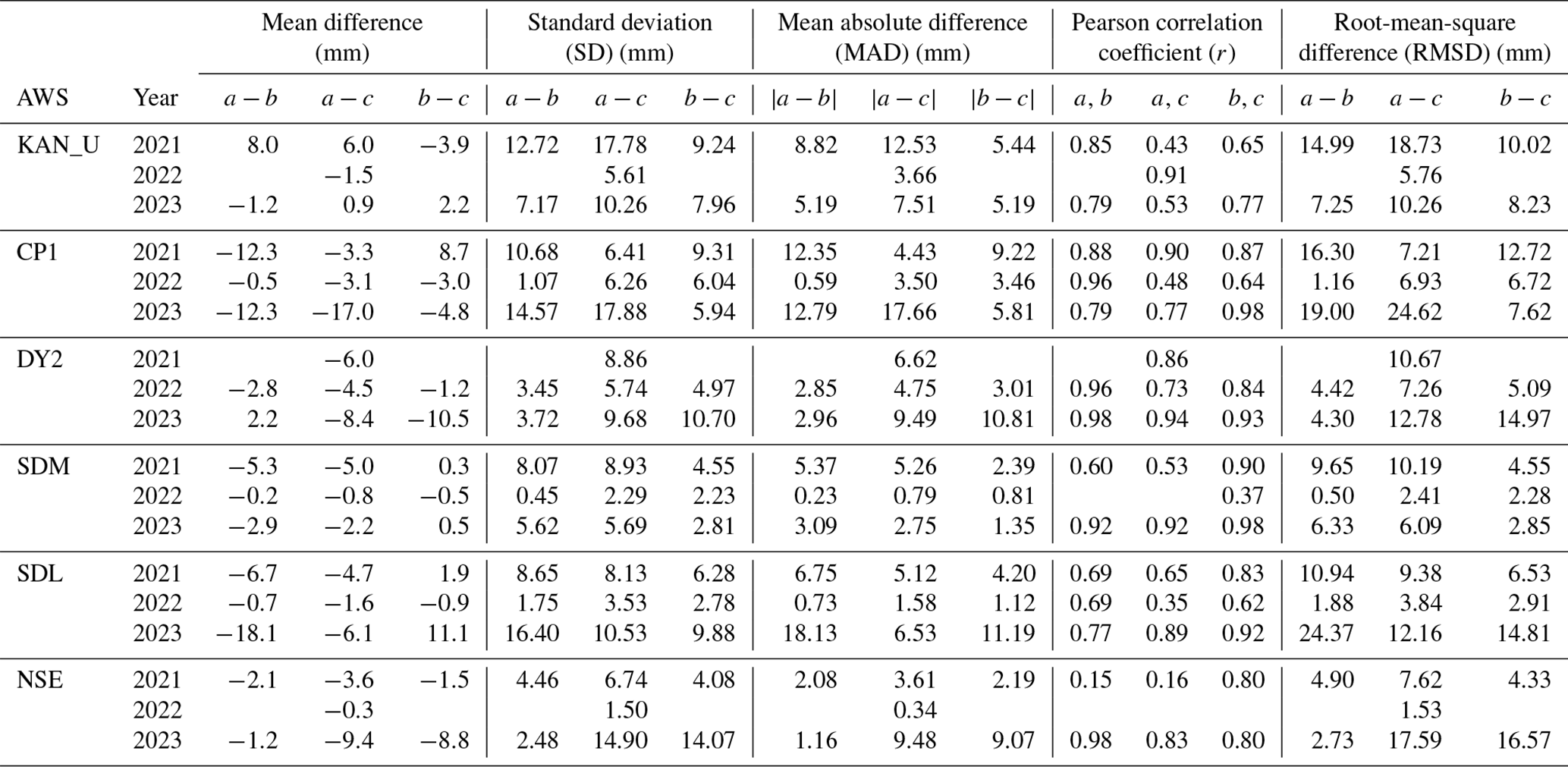
We performed a pairwise comparison among SMAP, EBM, and GEMB models (Fig. 6) for the 2021, 2022, and 2023 melt seasons (based on available meteorological data) at the six AWS locations. Performance metrics are documented in detail in Table 1 (mean difference, SD, mean absolute difference, Pearson linear correlation coefficient, and RMSD) and Table 2 (melt onset, freeze-up, duration of summer melt, maximum summer melt, and annual sum of daily LWA). Because of the SMAP outage for summer 2022, performance metrics in Table 1 only considered the operational part of SMAP. Table 2, however, excludes SMAP for the 2022 melt season except in the melt onset information, as the other metrics were impacted by the outage.

At the KAN_U site, the overall agreement between SMAP and the EBM was determined to be better (r>0.75) than the agreement between SMAP and the GEMB model (r<0.55) for the 2021 and 2023 melt seasons (Fig. 6a–c). All the AWS data required to run the EBM for the 2022 melt season were not available. GEMB used ERA5 data to gap-fill this period, and SMAP LWA closely aligns with GEMB estimates for the first part of the summer season until the outage. However, the GEMB model demonstrates earlier melt onset in the 2021 and 2023 melt seasons compared to both SMAP and the EBM. SMAP estimated a maximum summer melt of 56 mm at this site in the 2021 melt season, while both the EBM and GEMB models recorded a maximum summer melt of 30 and 45 mm, respectively, in the 2023 melt season. No pair shows consistent superiority at the CP1 site (Fig. 6d–f).

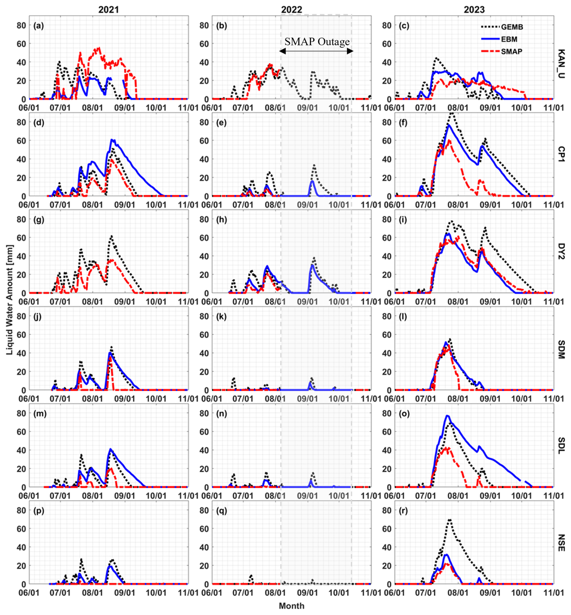
Figure 6 Comparison of the SMAP-retrieved total daily liquid water amount (dashed red lines) with the estimated LWA from the EBM (solid blue lines) and GEMB (dotted black lines) models at selected PROMICE and GC-Net AWSs within the GrIS percolation area. The SMAP data gap is depicted in shade for the 2022 summer season, and EBM results were not included when AWS data were missing where GEMB used ERA5 forcing.

SMAP LWA generally aligns closer with the GEMB model LWA in the 2021 melt season and with the EBM LWA in the 2022 melt season, whereas, in the 2023 melt season, the EBM and GEMB model match closer to each other than to SMAP. DY2 lacks AWS forcing during the 2021 melt season. Therefore, EBM results are missing for this melt season. Between SMAP and the GEMB model, the latter estimates more LWA overall (LWA_YS 1196 vs. 2101 mm), but there is a reasonable alignment between the peaks of the two LWA time series (Fig. 6g). The overall RMSD was found to be 10.67 mm. For the other two melt seasons (Fig. 6h–i), SMAP and the EBM results show superior agreements (r>0.96 and RMSD ∼4 mm). The GEMB model reports slightly higher LWA in 2023, both in magnitude and duration (4214 mm LWA_YS compared to 2893 mm (SMAP) and 2608 mm (EBM)), resulting in a higher overall RMSD (>12 mm) with the other two.

Table 1 Pairwise performance comparison among a (SMAP), b (EBM), and c (GEMB) models for the 2021–2023 summer seasons (1 June–31 October). Cells are left blank for missing SMAP or AWS data.

As per maximum summer melt and LWA_YS, SDL, SDM, and NSE sites experienced the highest LWA in the 2023 melt season compared to the other two melt seasons under consideration (Fig. 6j–r). SMAP did not record any LWA in any of these sites during the 2022 melt season, when the EBM (except NSE where AWS data were not available) and GEMB models also reported the smallest LWA in three melt seasons (Fig. 6k, n, and q). In the 2021 melt season, SMAP estimated an overall lower LWA and shorter summer melt duration than that of the EBM and GEMB models in these sites, but the agreements between EBM and GEMB models are in the same orders (see Tables 1 and 2), with both exhibiting delayed refreezing consistently compared to SMAP.

Table 2 Comparison of individual performances: (a) SMAP, (b) EBM, and (c) GEMB models. A threshold of 2 mm LWA was considered to avoid any spurious melt event. Comparisons were performed based on a daily matchup dataset. Cells are left blank when significant data were missing during summer.

3.1.3 SMAP LWA time series

Figure 7 shows the SMAP-retrieved LWA time series at the abovementioned six AWS locations on the southwestern and southeastern sides of the GrIS percolation zone. The time series does not include results during the 2019 and 2022 outages. As evidenced, the AWS sites in the southwestern sites (Fig. 7a–c) experienced more average LWA and longer summer melt duration than the AWS sites in the southeastern sites (Fig. 7d–f). SDL, SDM, and NSE witnessed an insignificant LWA (<10 mm) during the 2015–2020 melt seasons. However, it was found to be increasing in recent years (Fig. 7d–f). SMAP recorded the highest LWA in the 2023 melt season during 2015–2023 at all the AWS locations, except at KAN_U, where 2021 marked the highest melt season.

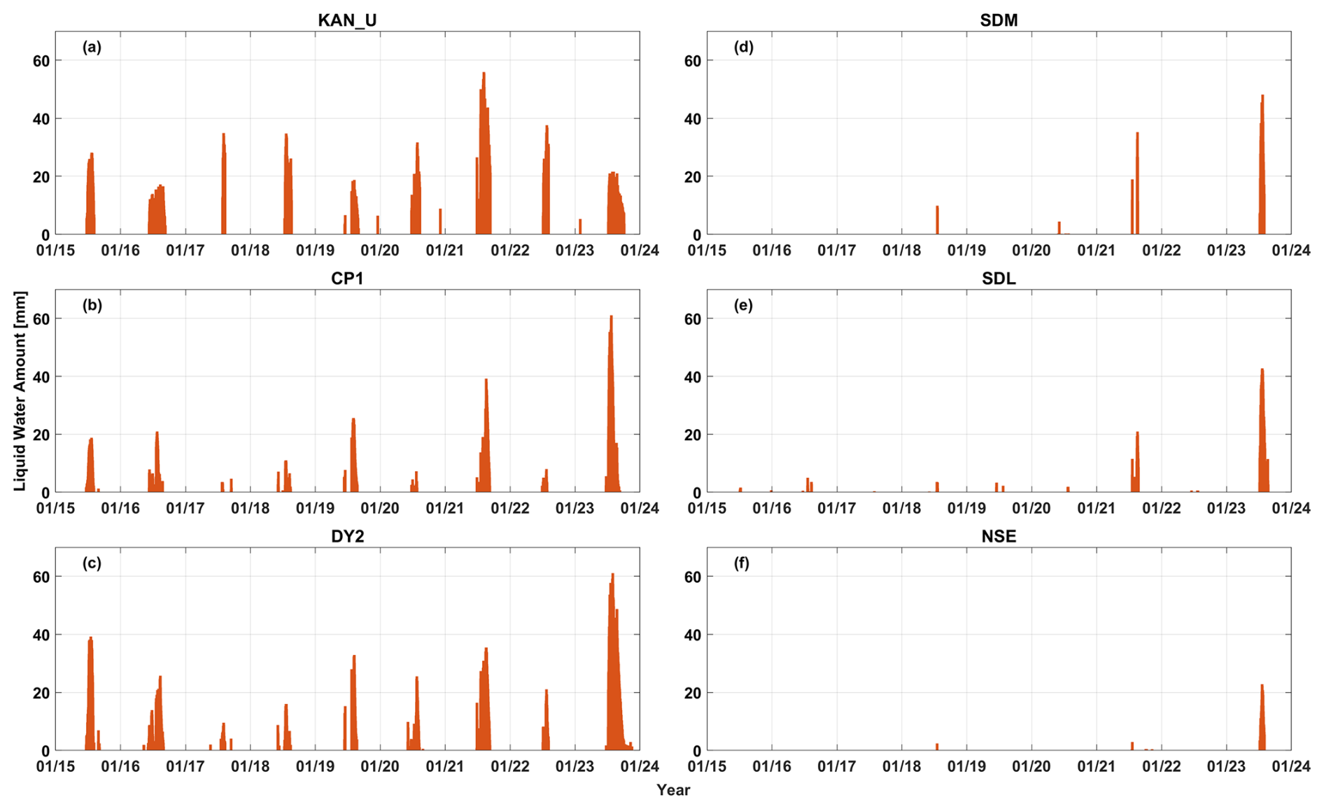
Figure 7 SMAP-retrieved LWA time series for the 2015–2023 period at six selected PROMICE and GC-Net AWSs within the GrIS percolation area.

3.1.4 Spatial variability

Figure 8 illustrates the annual sum of daily LWA (LWA_YS) for 2015–2023. Here, we masked the area where melt is detected by decreasing summer T_B (compared to winter reference). As mentioned in Sect. 2.2.3, the current LWA quantification algorithm applies to increasing T_B only. This excluded the melt flags in the ablation zone and upper accumulation zone, as indicated by gray shades in Fig. 8. There were also some occasions when summer T_B decreased below the winter threshold in the percolation, too. Those anomalies were probably caused by short-lived melt events that refroze between SMAP passes and impacted T_B. These anomalies are also masked and not included in the results. As depicted, SMAP captured the similar spatial trends of LWA distribution across the percolation zone of the GrIS as reported by previous studies (van den Broeke et al., 2016; Houtz et al., 2021). In the time frame under consideration, the 2023 melt season (Fig. 8i) had the highest LWA_YS (2634 mm on average for the percolation area), while 2017 (Fig. 8c) had the lowest value (757 mm on average for the percolation area). In 2015 (Fig. 8a), the northern ice sheet exhibited a relatively high LWA_YS; similar intensity and extent were also recorded for 2023 (Fig. 8i). Notably, the melt extended to upper elevations in the dry snow zone in 2021 and 2023. Unfortunately, SMAP outages in 2019 (Fig. 8e) and 2022 (Fig. 8h), led to incomplete coverage for those years and lower LWA_YS. It is worthwhile to reiterate that the integrated LWA is a measure of the total seasonal LWA in the specified area.

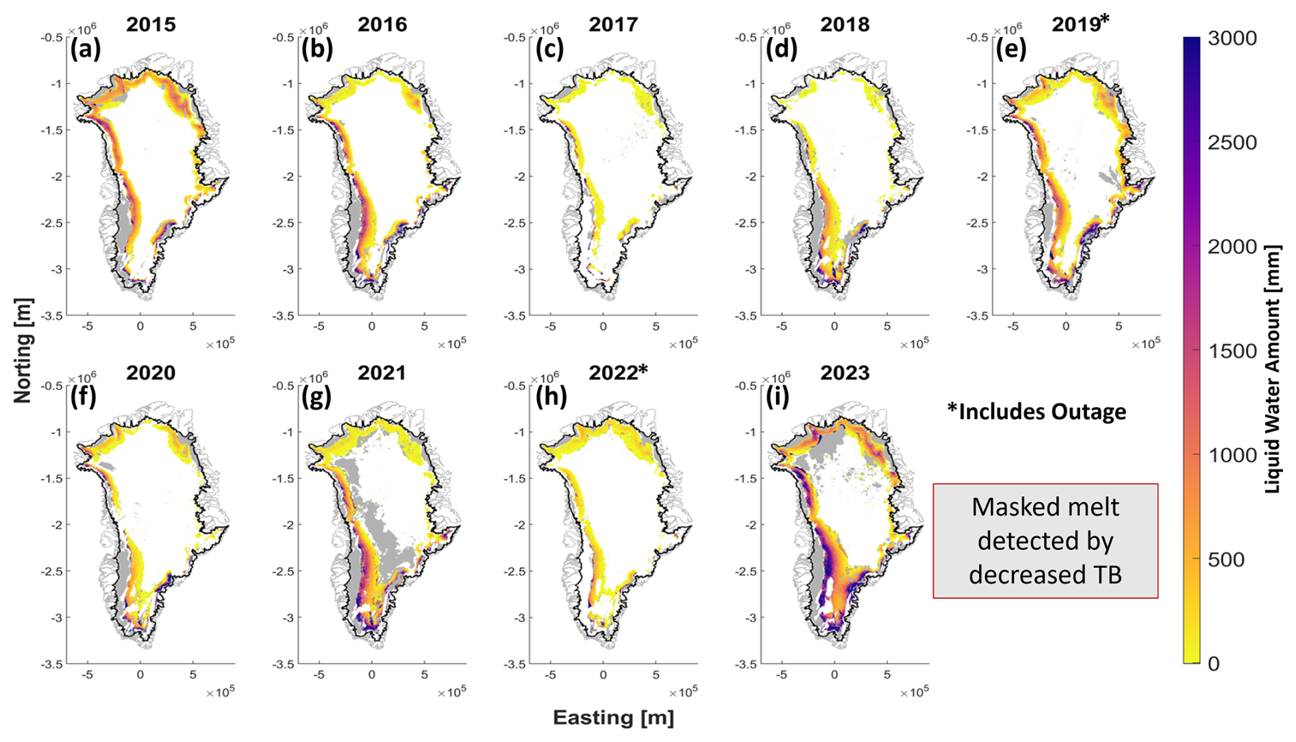
Figure 8 Total annual sum of SMAP daily LWA for 2015–2023. The solid black line represents GrIS edges, and the gray color masks inside the ice sheet indicate melt detections by decreasing T_B, which were not quantified.

4 Discussion

The L-band radiometry has the unique advantage of receiving the emission from the deep layers of ice sheets, offering the opportunity to track meltwater from deeper layers. We have demonstrated its capability to estimate the seasonal LWA that generally agrees with two state-of-the-art ice sheet models, forced with independent in situ AWS measurements. The legitimacy of spatial and temporal variability shown in SMAP retrieval for the percolation area of the GrIS is promising.

There are some disagreements as well, but those do not necessarily indicate a deficiency in the SMAP retrievals, since both the references are models with their own limitations. The differences between model results and SMAP retrievals are not systematic, so they are difficult to explain, but there is no evidence of a consistent bias. Nonetheless, some of the discrepancies between these estimations of LWA stem from the scale at which those datasets operate. The SMAP LWA was estimated from the T_B measurements averaged over a large footprint and a short integration time. Furthermore, rSIR enhanced-resolution data products involve overlapping observations to produce the 3.125 km gridded data but still have an effective spatial resolution of ∼30 km. Thus, they represents near-instantaneous vertically integrated LWA, averaged over the grid point, whereas the AWS data are the hourly average of “point” measurements representative of the 0.1–1 km surrounding the station. The total LWA from AWS-forced data is the hourly averaged, vertically integrated net water balance which is determined as the cumulative sum of hourly surface melt generation, refreezing, and drainage. The surface melt generation is driven by the net surface energy balance (net radiation and turbulent heat fluxes), which involves uncertainties (e.g., the surface albedo and roughness, errors in the meteorological inputs), while how the melt and heat are distributed in subsurface firn involves additional uncertainties, including sensitivity to initial conditions (e.g., the firn temperature and density profile; Samimi et al., 2020). These models transform surface meteorological information into an amount of surface melt relying on loosely constrained parameterizations (Covi et al., 2023). Eventually, the models' formulation for the meltwater infiltration is still poorly constrained (e.g., Vandecrux et al., 2020). Additionally, both the models we used (like other state-of-the-art firn models) are one-dimensional: they only consider vertical movement of water and heat and do not account for horizontal advection. However, firn hydrological processes are complex and heterogeneous, and processes such as ice layer formation are intrinsically three-dimensional. What the models consider to be “drainage” (meltwater that moves out of the system) both vertically and horizontally could still be within the SMAP sensing depth and horizontal footprints. Hence, the comparison should be considered accordingly.

One important disagreement between SMAP and EBM LWA estimation, especially during the refreezing periods, is that EBM retained LWA for an extended period when SMAP showed completely refrozen conditions (Fig. 6). We used SUMup subsurface temperature measurements (Vandecrux et al., 2024a) to verify the cases for which SUMup data are available. One example is shown in Fig. 9. It compares the model-estimated subsurface temperature (Fig. 9a) corresponding to the 2021 LWA at CP1 (Fig. 6d) to the in situ measured subsurface temperature (Fig. 9b). It is evident that, although the penetration depth of the model wetting front closely matches the observation, the measurement demonstrates a higher and faster refreezing compared to the model. The subsurface measurement shows fully refrozen conditions by early September (closely agreeing with what was revealed by SMAP; see Fig. 6d). However, the model seems to retain the subsurface meltwater with a persistent wetting front even past the beginning of October, which seems unlikely. Speculating extra melt production due to possible error in the AWS surface forcing, and other surface processes in the EBM, we examined the modeled subsurface temperature profile by reducing surface melt with different factors (<1). We also performed similar analysis with irreducible water content and thermal conductivity. In either case (not shown), we could not match the subsurface profile with the measured profile within reasonable agreements. This incites questions regarding the model representation of meltwater infiltration, heat transfer, and refreezing.

The models do not include meltwater infiltration by finger flow (piping). Some recent studies have shown that this is an important mechanism for moving liquid water from the surface to deep depths (e.g., Vandecrux et al., 2020). The piping events are short-lived penetration and refreezing events. SMAP will measure the LWC in the piping event, even when it passes the wetting front, unless the water is refrozen before the SMAP measurement (as is the case with all short-lived melt events). The model would calculate a certain amount of meltwater based on the surface energy balance, and it would put all this water into the wetting front layer. However, from the literature and as confirmed by the subsurface temperature measurements (Fig. 9b), some fraction of this water would be partitioned into deep piping. The model only includes top-down migration of a wetting front. This may explain why there are discrepancies between the modeled subsurface temperature profile and the observed subsurface temperature profile in some cases. Indeed, the deep penetration events causing warming spikes beyond the wetting front distort the temperature profiles. Therefore, some differences between SMAP and the EBM and GEMB models could be attributed to this weakness in process representation in the model, but, overall, these problems are multifaceted, and additional work is required to understand the basis for these discrepancies. However, to this day, there is no observational dataset that allows us to evaluate directly the LWA retrieved from satellite observations or calculated by a snow and firn model.

Besides the coarser spatial resolution, the SMAP algorithm has its own shortcomings. The emission model simulated T_B with a simplified view of the stratigraphy which lacks detailed representation of snow and firn microstructures. The model also neglected atmospheric contributions and assumed a homogenous medium and smooth surface within each layer. Although these effects are not significant at the L-band, a detailed characterization was not performed. The detection algorithm follows a threshold-based technique that uses the winter reference of the T_B to detect melt events. As a result, it is capable of quantifying the seasonal LWA only, not the LWA in perennial firn aquifers which store a large quantity of saturated liquid water on the GrIS throughout the year (Montgomery et al., 2017; Miller et al., 2020b, a). Miller et al. (2022a, b) developed an empirical technique to map Greenland's perennial firn aquifers with SMAP L-band brightness temperature; however, without complementary observations of firn aquifers via other means such as radar sounding, while the detection itself is ambiguous, the quantification would be more challenging. The current algorithm also excluded areas where T_B decreases during summer melt. Future work will be continued to overcome some of these limitations and refine the algorithm.

To extend the algorithm for GrIS-wide LWA quantification, the ablation zone presents a major challenge. Although SMAP can detect melt events in the ablation zone, the quantification is difficult for several reasons. The hydrological features of the ablation zone are markedly different from the percolation or upper accumulation zone. There are widespread networks of many supraglacial lakes and rivers, crevasses, and other complex heterogeneous factors, such as surface topography, dust deposition, and slush saturation (Cooper and Smith, 2019; Poinar and Andrews, 2021; Smith et al., 2017). This generates an intricate radiometric response. The average LWA in the ablation zone is also significantly higher limiting the L-band emission in the upper layer only. Houtz et al. (2019) used L-band observations from the SMOS satellite to derive LWA at the Swiss Camp GC-Net AWS located in the ablation zone with a simplistic assumption of fixed (10 cm) wet-layer thickness. More in situ observations are needed to characterize the spatial and temporal variability in LWA in the ablation zone.

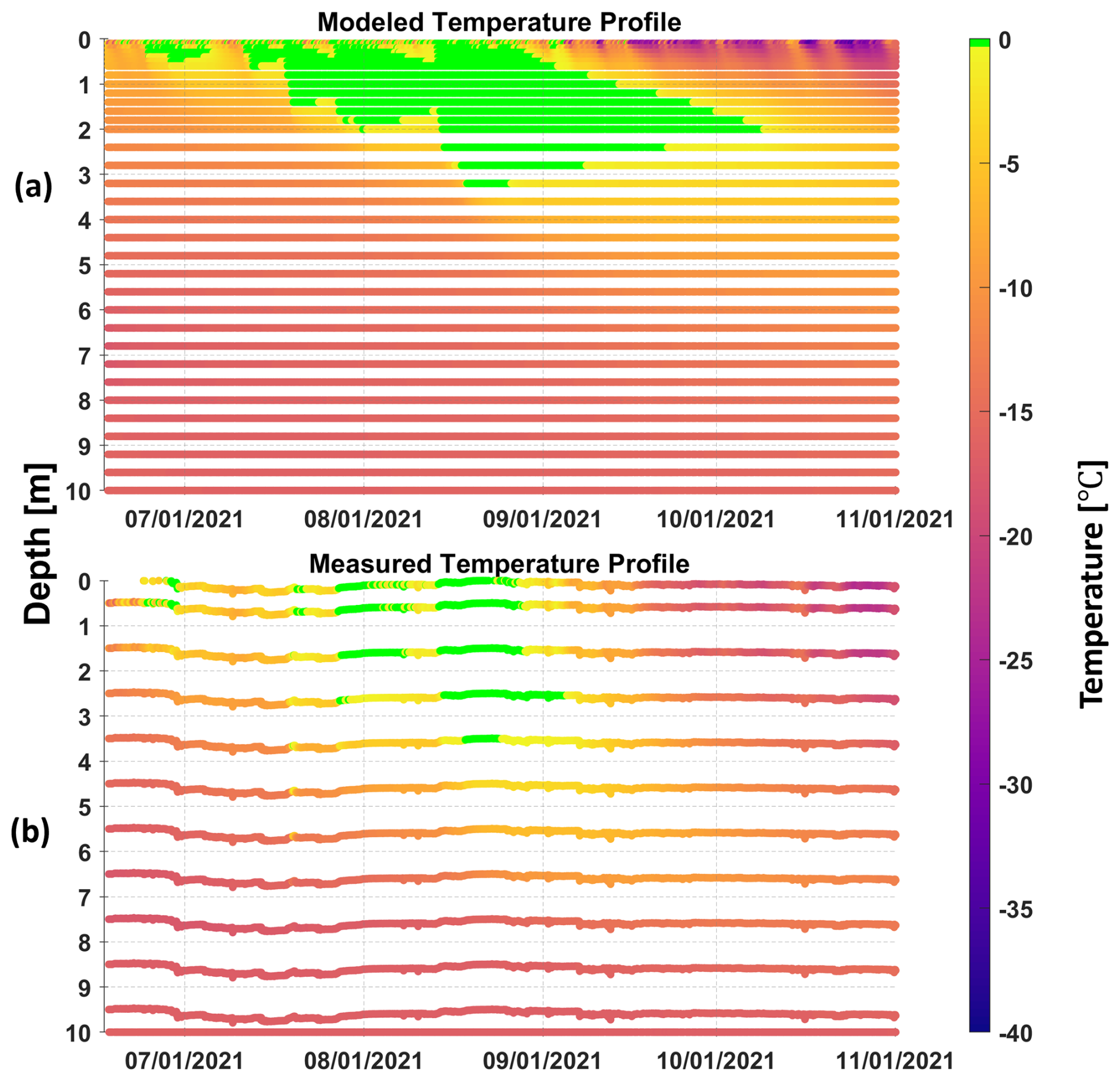
Figure 9 Modeled (a) and measured (b) subsurface temperatures corresponding to total LWA at the CP1 site during the 2021 melt season. The 0°C isotherm is highlighted in green.

5 Conclusion

We have demonstrated quantification of the total surface and subsurface meltwater amount over the Greenland ice sheet using the L-band radiometric observations from the SMAP mission. The retrieval algorithm was described, and the validation results with six in situ weather station measurements and reanalysis data were provided. The comparison results were analyzed, showing that the retrieval generally agrees with the AWS-driven LWA across the percolation zone. The model uncertainties in representing firn hydrological and thermal processes were explored, and the greatest differences involve the timescale for internal refreezing. The model results commonly predict a longer season for liquid water content in the snow and near-surface firn, i.e., delays in refreezing relative to the SMAP data. Limitations of the LWA of SMAP and model estimates, and possible reasons for the discrepancies between them, were discussed. Further work is required to understand the basis for these discrepancies and refine the algorithm. A detailed sensitivity analysis and uncertainty characterization of the LWA retrieval algorithm, including dielectric mixing models, is required. The results demonstrate the potential for providing an observational dataset at timescales and space scales that will advance our understanding of ice sheet physical processes, helping to better project Greenland's contribution to global sea level rise in response to climate change and variability. To create a longer time data product, integrating SMOS observations (2010–present) with SMAP will be beneficial. The algorithm can easily be extended for LWA estimation in the Antarctic ice sheet. ESA's upcoming Copernicus Imaging Microwave Radiometer (CIMR) mission (to be launched in 2029) will include coincident L (1.4 GHz) to Ka (36 GHz) channels for the first time (Colliander et al., 2024; Kilic et al., 2018). Future works should explore the added benefits of other complementary frequencies (6 GHz up to 36 GHz bands) in order to provide a possible depth profile of the LWC.