Developing a deep learning forecasting system for short-term and high-resolution prediction of sea ice concentration

There has been a steady increase in marine activity throughout the Arctic Ocean during the last few decades, and maritime end users are requesting skilful high-resolution sea ice forecasts to ensure operational safety. Different studies have demonstrated the effectiveness of utilizing computationally lightweight deep learning models to predict sea ice properties in the Arctic. In this study, we utilize operational atmospheric forecasts, ice charts, and sea ice concentration passive microwave observations as predictors to train a deep learning model with future ice charts as ground truth. The developed deep learning forecasting system predicts regional ice charts covering parts of the East Greenland and Barents seas at 1 km resolution for 1–3 d lead time. We validate the deep learning system performance by evaluating the position of forecasted sea ice concentration contours at different concentration thresholds. It is shown that the deep learning forecasting system achieves a lower error for several sea ice concentration contours when compared against baseline forecasts (persistence forecasts, sea ice free drift, and a linear trend) and two state-of-the-art dynamical sea ice forecasting systems (neXtSIM and Barents-2.5) for all considered lead times and seasons.

1 Introduction

Arctic sea ice thickness and extent have decreased since the first satellite observations were obtained (Kwok, 2018; Serreze and Meier, 2019) as a response to climate change (Notz and Marotzke, 2012), which is amplified in the Arctic region (Serreze and Barry, 2011). Summer months are experiencing the greatest loss of sea ice extent (Comiso et al., 2017), with models from the Coupled Model Intercomparison Project 6 (CMIP6) projecting the first virtually ice-free ($<\mathrm{1}\times {\mathrm{10}}^{\mathrm{6}}$ km²) Arctic summer before 2050 (Notz and Community, 2020). As a consequence of the sea ice retreat during the summer months, there has been an increase in maritime activity in the Arctic (Eguíluz et al., 2016; Gunnarsson, 2021), resulting in a consistent increase in the number of ships present in the Arctic. The period during which many vessels operate has also extended beyond the summer months, increasing mariners' exposure to hazardous sea ice conditions (Müller et al., 2023). The influx of operators to the Arctic region has increased the demand for accurate short-range sea ice forecasts (Stocker et al., 2020) and for end users' needs to be taken into account during the validation of these forecasts (Melsom et al., 2019; Wagner et al., 2020).

Although dynamical sea ice forecasting systems have been producing operational forecasts at different resolutions and lead times (Sakov et al., 2012; Metzger et al., 2014; Williams et al., 2021; Röhrs et al., 2023), feedback from maritime operators suggests that current sea ice forecasts lack sufficient and relevant verification (Veland et al., 2021). Consequently, maritime operators tend to rather rely on their own experience (Blair et al., 2022), despite the improved situational awareness provided by sea ice forecasts for tactical navigation (Rainville et al., 2020). Moreover, dynamical forecasts are computationally expensive, especially when targeting high spatial resolutions. In recent years, statistical forecasting approaches have emerged where deep neural networks have been trained on past sea ice information and the state of the atmosphere in order to predict the future state of sea ice concentration (SIC) (e.g. Fritzner et al., 2020; Liu et al., 2021b; Andersson et al., 2021; Liu et al., 2021a; Ren et al., 2022; Grigoryev et al., 2022). These machine learning approaches require little memory and computational resources to produce a forecast, once they are trained.

Previous studies (Liu et al., 2021b; Andersson et al., 2021; Liu et al., 2021a; Ren et al., 2022) have trained deep learning models on reanalysis datasets such as ERA5 (0.25° resolution) (Hersbach et al., 2020) or have used SIC derived from coarse-resolution (25 km resolution) satellite climate data records (such as the products from Cavalieri et al., 1996, and Lavergne et al., 2019). Andersson et al. (2021) proposed IceNet, a pan-Arctic U-Net classifying SIC into separate classes defined by sea ice concentration thresholds. Andersson et al. (2021) demonstrated that IceNet consistently improved upon the seasonal numerical forecasting system SEAS5 (Johnson et al., 2019) for lead times of 2 months and longer. Similarly, Liu et al. (2021b) showed that a convolutional long short-term memory network covering the Barents Sea with a 6-week lead time directly predicting SIC was more skilful than persistence for all considered weekly lead times. However, due to the aforementioned models using climatological-scale data as predictors and ground truth, their application to maritime users as short-term operational forecasts is limited (Wagner et al., 2020).

Grigoryev et al. (2022) presented a multi-regional U-Net forecasting system predicting SIC for lead times of up to 10 d, where the real-time availability of SIC satellite retrievals and numerical weather forecasts was considered. The deep learning forecasts of Grigoryev et al. (2022) considerably outperformed persistence and linear trend baseline forecasts in the considered regions of the Barents, Labrador, and Laptev seas. Fritzner et al. (2020) demonstrated the possibility of utilizing a fully convolutional network to forecast ice charts for the region around Svalbard and the Barents Sea; however the forecasts had a coarse spatial resolution due to limited computational resources. High-resolution sea ice forecasts are important for this region as it is the focus of many commercial operators from different maritime sectors, such as shipping, fishing, and tourism (Stocker et al., 2020; Müller et al., 2023).

In this paper we present the development of a regional deep learning forecasting system targeting 1 km spatial resolution and 1–3 d lead time, covering the area around Svalbard and the Barents Sea. The choice of predictors and target data is made with operational concerns, and the quality of the forecasts is assessed against relevant baseline forecasts and dynamical sea ice forecasting systems in a manner relevant for end users (Melsom et al., 2019; Wagner et al., 2020). The impact from the different predictors is also assessed. Section 2 describes the datasets used for this study, followed by Sect. 3, which presents the neural network implementation and verification setup. Section 4 presents the results, with Sect. 5 providing the discussions and conclusions.

2 Data

To develop the deep learning forecasting system, several observation and physical model forecasting system datasets have been chosen as predictors, as targets, and for validation. When selecting appropriate datasets, their spatial resolution and release frequency are considered in order to develop an operational product. Table 1 presents the different products we used and the role they play in our forecasting system, which are further described in the following sections. The region of interest is depicted in Fig. 1 and is constructed as an intersection between the regional domains of the gridded ice chart data produced by the Norwegian Ice Service (https://cryo.met.no/en/latest-ice-charts, last access: 15 September 2023) and the regional numerical weather prediction system AROME Arctic (Müller et al., 2017). The deep learning model has been developed using the U-Net architecture (Ronneberger et al., 2015), which requires the spatial dimensions of the input fields to be repeatedly divisible by a given factor a number of times. For simplicity, the model domain was set to be a 1 km spatial resolution square grid containing 1792×1792 equidistant grid cells, which is divisible by 4 a total of 4 times. This domain was achieved by removing lower latitudes from the original AROME Arctic domain, affecting the southern Norwegian, Barents, and Kara seas.

Table 1 Products used, their application, and their temporal regime. Observational products and physical forecasting models are separated by the descriptive italic text. Time regime refers to the time period that the dataset covers with respect to the initialization date of the deep learning model.

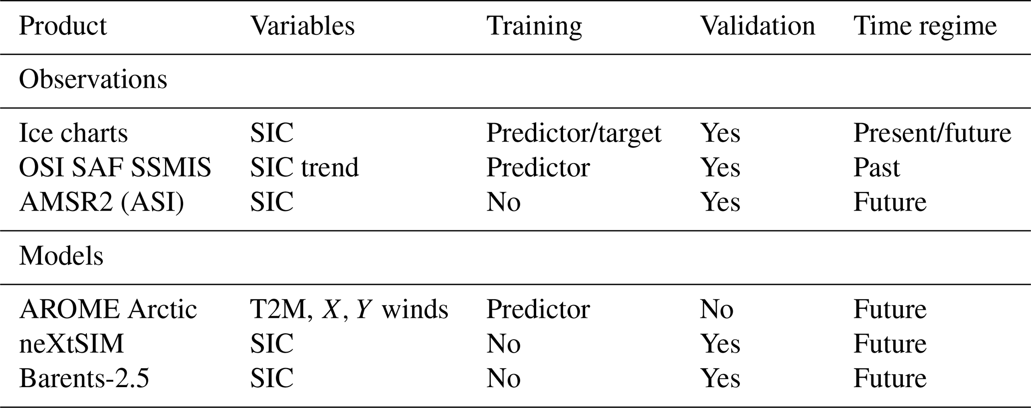
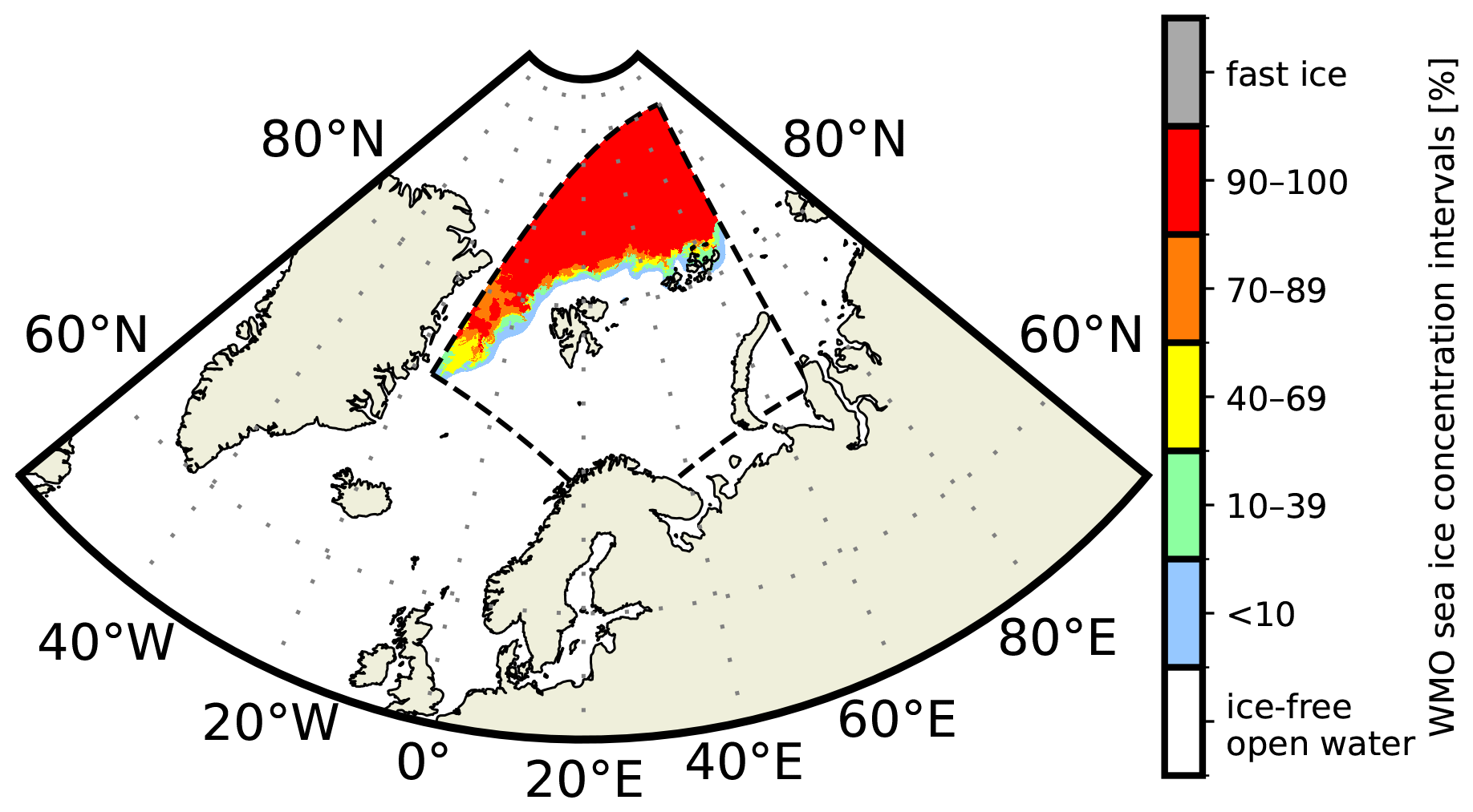
Figure 1 The model domain (dashed contour) together with the SIC retrieved from a ice chart (15 September 2022). The SIC intervals and colour code follow the WMO Ice Chart Colour Standard and Sea Ice Nomenclature.

2.1 Sea ice concentration observations

The ice charts are manually drawn to deliver a SIC product which is distributed every workday at 15:00 UTC by the Ice Service of the Norwegian Meteorological Institute (https://www.cryo.met.no/en/latest-ice-charts, last access: 15 September 2023). The ice analyst who draws the ice chart assesses and merges available synthetic aperture radar (SAR) scenes with visible and infrared imager observations. These data sources are supplemented by coarse-resolution passive microwave observations to achieve a consistent spatial coverage. Incoming observations are interpreted by the ice analyst as they become available. For our model domain (Fig. 1), Sentinel-1 SAR swaths are available between midnight and 08:00 UTC starting from Novaya Zemlya. Following consideration of input data availability and the ice analyst's judgement, we assume the ice charts reflect the sea ice state at 12:00 UTC.

We use gridded SIC from the ice charts as both a predictor representing initial sea ice conditions and a target at 1–3 d lead time since the product captures daily (weekdays from Monday to Friday) observed SIC at a high (<1 km) spatial resolution. The ice charts are a categorical product, with SIC following the World Meteorological Organization (WMO) total concentration intervals (see colour bar of Fig. 1). For this study, the ice charts have been gridded from vector polygons onto the model domain with a 1 km spatial resolution using nearest neighbour interpolation. Moreover, we have filtered out Baltic Sea sea ice, as the task of the deep learning system in this study is to predict sea ice in the Greenland and Barents seas.

In addition to the ice charts, SIC observations from the Ocean and Sea Ice Satellite Application Facility (OSI SAF) special sensor microwave imager/sounder (SSMIS) (OSI-401) and AMSR2 observations processed with the ASI algorithm from the University of Bremen (Spreen et al., 2008) are utilized. OSI SAF SSMIS is supplied on a 10 km spatial resolution and is used to compute a linear sea ice concentration trend, which serves as both a predictor and a baseline forecast for validation. Motivated by the lack of temporal awareness of the U-Net architecture (Ronneberger et al., 2015), computing a linear trend from past sea ice concentration fields will encode multiple previous time steps into a single two-dimensional field. Moreover, computing the linear trend from a product other than the ice charts will supply the model with correlated but not overlapping information. It is also noted that the ice charts are not produced every day; hence it would not be possible to use the product to compute a local trend.

AMSR2 observations are used for validation of the deep learning forecasting system only. The AMSR2 data utilized for this work are the ASI sea ice concentration product from the University of Bremen (Spreen et al., 2008). The dataset is provided on a 6.25 km grid. AMSR2 observations can be considered an independent product from the ice charts, which are primarily derived from SAR observations and are not used to train the deep learning model. Hence, the AMSR2 data are used as an external product for validation of forecast performance, providing an estimation of the deep learning model's ability to provide consistent forecasts beyond using the ice charts as validation.

2.2 Physical forecasting systems

In addition to training the deep learning model on current and previous sea ice concentration data, we also include atmospheric predictors as it has been demonstrated that the inclusion of the present and future state of the atmosphere can improve sea ice predictions from deep learning (Grigoryev et al., 2022; Palerme et al., 2024). For this study, forecasts of 2 m temperature and 10 m wind components, adjusted to align with the x,y dimensions of the model grid (x,y wind), were taken from the AROME Arctic regional numerical weather prediction system developed for operations at the Norwegian Meteorological Institute (Müller et al., 2017). Although it is not a forecast field, the land–sea mask used in AROME Arctic is also extracted as a predictor. We use AROME Arctic forecasts as predictors for this study due to its high spatial resolution and regional coverage of the European Arctic. AROME Arctic runs up to a 66 h lead time, is supplied on a 2.5 km resolution grid with 66 vertical levels, and initiates a new forecast every 6 h. Near-surface winds influence the sea ice drift following a non-linear relationship between wind speed, sea ice drift speed, sea ice concentration, and sea ice thickness (Yu et al., 2020). Moreover, near-surface temperatures affect the sea ice through melting or growth. AROME Arctic has been in operation and continuous development since October 2015, routinely receiving updates, which introduce permanent bias changes for predicted variables. Due to a major change to the representation of snow over sea ice in 2018, a warm bias in near-surface temperatures above sea ice was significantly reduced in the model (Batrak and Müller, 2019). Thus, we start our training dataset in 2019 to avoid supplying our deep learning model with samples containing different temperature biases, especially close to the marginal ice zone (MIZ), where the greatest model response to predictors occurs.

Moreover, two short-range sea ice forecasting systems, neXtSIM-F (Williams et al., 2021) and Barents-2.5 (Röhrs et al., 2023), are used to validate the deep learning forecasts against high-resolution physical forecasting systems. neXtSIM-F is based on the neXtSIM sea ice model, which is a dynamical/thermodynamical sea ice model using a brittle rheology (Rampal et al., 2016). The version of neXtSIM used for this work uses the brittle Bingham–Maxwell rheology (Ólason et al., 2022). neXtSIM receives oceanic forcing from TOPAZ4 (Sakov et al., 2012) and atmospheric forcing from ECMWF IFS (Owens and Hewson, 2018). The forecasts are supplied on a pan-Arctic grid at 3 km resolution. Barents-2.5 is a regional ocean and sea ice ensemble forecasting system developed at the Norwegian Meteorological Institute (Röhrs et al., 2023) and is produced on a 2.5 km spatial resolution and runs up to a 66 h lead time on the same grid as AROME Arctic. The sea ice model used in Barents-2.5 is CICE (Hunke et al., 2015). At prediction time, six members are initiated, with one member receiving atmospheric forcing from AROME Arctic and the rest from atmospheric forecasts from ECMWF; however for this study only the member forced by AROME Arctic has been considered. Finally, due to recent developments of the model, only forecasts starting from June 2022 have been considered from Barents-2.5.

3 Methodology

3.1 Dataset preprocessing and selection

We perform preliminary computations in order to ensure that the data from different sources are on a common grid. The data preprocessing is performed in two stages. Firstly, data not matching the AROME Arctic projection are reprojected. Secondly, for data available at a coarser resolution, nearest neighbour interpolation is performed in order to resample the data onto a 1 km grid. The U-Net architecture requires all predictors to have valid values in all grid cells; however the input, target ice charts, and SIC trend do not consistently represent SIC for land-covered grid cells due to their intended unavailability. In order to avoid sharp gradients between sea-ice-covered seas and land-covered areas in the ice charts and SIC trend, we apply a nearest neighbour interpolation of the local sea ice conditions to fill in the missing sea ice concentration over land grid points following Wang et al. (2017).

Since all the datasets we use for training come from operational products, we have to take production time, publishing time, and forecast length into account when selecting predictors. A graphical summary of the operational schedule for predictor selection is shown in Fig. 2. The ice charts are valid at 12:00 UTC, which is regarded as the initialization time for the deep learning forecasts. The OSI SAF linear trend is computed from the 5 previous days, until the day before deep learning forecast initialization. We want AROME Arctic forecasts to provide the future state of the atmosphere to the deep learning system, which we set to lead times beyond the deep learning initialization time. Hence, it follows that the atmospheric forecast should cover the time between the input and target ice chart valid time.

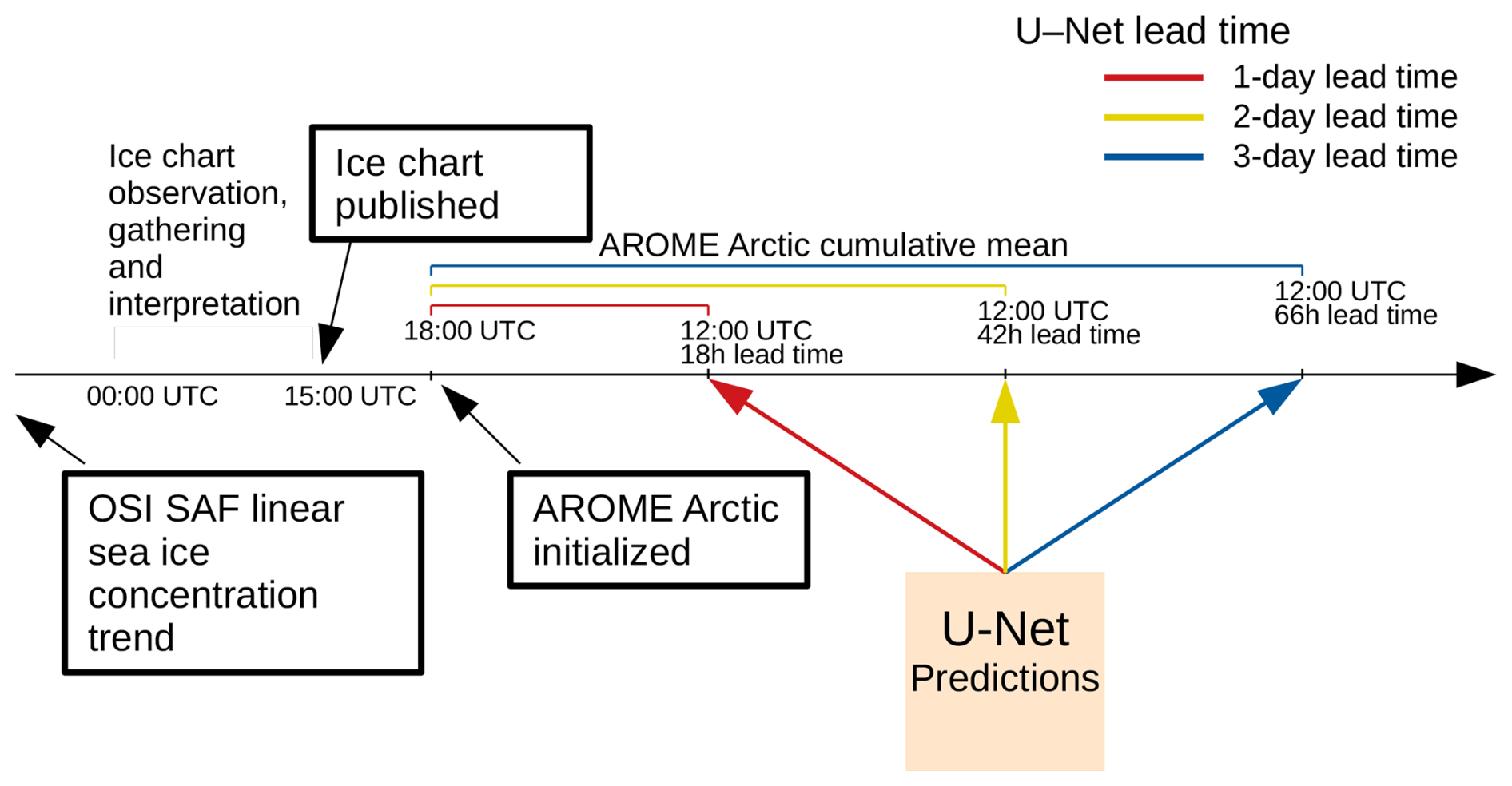
Figure 2 Overview diagram describing predictor publication scheduling, selection, and preprocessing. Description of when the different predictors are published in relation to a published ice chart when constructing a single sample for a given date. The ice charts are published at 15:00 UTC, followed by AROME Arctic initialized at 18:00 UTC (available ∼20:30 UTC). The different colours refer to the deep learning forecast lead time.

We choose to use AROME Arctic forecasts initiated at 18:00 UTC on the same day as ice chart publication. Furthermore, we set the AROME Arctic forecast reference time to be 12:00 UTC on the prediction day, regardless of the model lead time of 1, 2, or 3 d. This way, we ensure that atmospheric forecasts cover the time period in between the ice chart publication and intended target lead time. Moreover, AROME Arctic initiated at 18:00 UTC reaches 12:00 UTC for a 3 d target lead time after 66 h (the longest lead time available from AROME Arctic forecasts), which motivates the choice of having 12:00 UTC as the reference time regardless of the target lead time. In addition, AROME Arctic has a production time of about 2.5 h, which ensures that forecasts initiated at 18:00 UTC are available before midnight, allowing deep learning forecasts to be published on the same day as the input ice chart.

When selecting atmospheric forecasts initiated at 18:00 UTC, 6 h of future atmospheric development occurring after the ice chart valid time (12:00 UTC) is not included in the atmospheric predictors. Although AROME Arctic is also initiated at 12:00 UTC, the forecast initiated at 18:00 UTC is more up to date and, as such, is assumed to be more reliable, especially at longer lead times. Moreover, the impact of appending 6 h of AROME Arctic initialized at 12:00 UTC to the training data has been tested and was shown to have an insignificant impact on model performance (see the Supplement). Finally, the ice charts do not represent the sea ice state at any given lead time; rather, they are a mean representation of previous observations accumulated over time, ending at publication time. Hence, regardless of AROME Arctic initialization time, we assume that there will be some irreducible timing difference between the sea ice state from the ice charts and the initial atmospheric state from AROME Arctic, which also varies spatially.

Instead of loading multiple high-resolution AROME Arctic fields during training, we preprocess atmospheric variables during dataset creation to reduce the amount of memory needed to load predictors during training. We reduce the atmospheric forecast fields between the start date and 12:00 UTC on the target date along the temporal dimension into a mean field. In addition to reducing the memory footprint of each predictor, reducing the time steps into a mean value field also accumulates the temporal changes in each atmospheric variable into a single predictor. Aggregating statistics at an increasing temporal range causes atmospheric predictors to be dependent on target lead time. Hence, deep learning models are trained independently for each target lead time.

The main dataset we use covers the period between 2019–2022. We further split the data such that 2019–2020 is used for training, 2021 is used for validation, and 2022 is the test dataset. Table 2 provides an overview of the number of available samples for each year given each model target lead time. Moreover, the predictors are normalized according to the min–max normalization equation. This normalization scheme ensures that the different predictors are in the same numerical range [0,1] and that predictors can be drawn from non-normal distributions such as the ice charts. Finally, with this scheme we can combine categorical predictors from the ice charts with continuous predictors from AROME Arctic.

Table 2 Subset affiliation and number of samples for each year over the different target lead times.

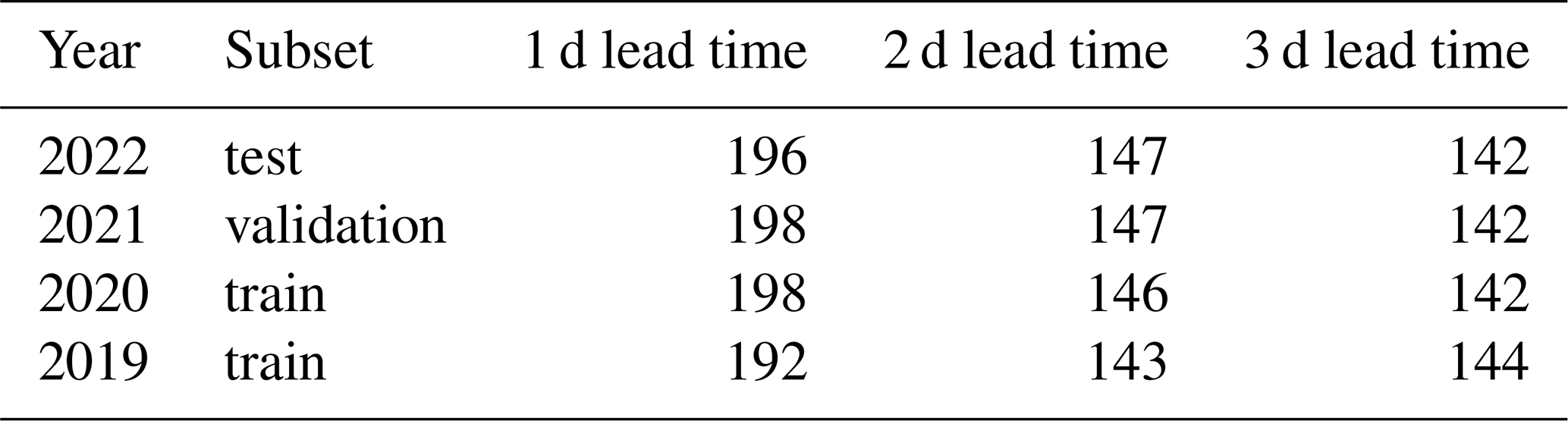
Due to the routine lack of ice charts during weekends, there is a limited number of dates that can be used for training and verification, and the sample size depends on lead time, as shown in Table 2. Comparing the similarly sized 2 and 3 d lead time datasets against the number of samples at 1 d lead time reveals an approximate 25 % reduction in the number of available dates that is consistent for all considered years. This has implications when the ice charts are used to evaluate deep learning forecast performance because verification scores for models targeting different lead times are computed from different sets of dates.

3.2 Cumulative contours

Norwegian ice charts represent SIC in unevenly sized concentration categories; hence we treat the prediction of an ice chart as a classification task. For automated ice charting, Kucik and Stokholm (2023) have reported that the categorical cross-entropy loss function achieves the highest rate of true positive predictions. However, ice charts are heavily imbalanced fields mostly populated with ice-free open water (0 %) and very close drift ice (≥90 %), and neural networks trained with categorical cross-entropy tend to prioritize predicting the most frequently occurring classes, while making fewer true positive predictions for intermediate SIC categories (Kucik and Stokholm, 2023).

Motivated by the skewed SIC distribution between the categories, which constitutes the MIZ, we reformulate the target SIC such that each category is defined cumulatively and predicted independently using the six SIC thresholds, 0 %, 10 %, 40 %, 70 %, 90 %, and fast ice (as shown in Fig. 1). Cumulative contours are a novel reformulation of the SIC prediction task, which aims to preserve the ice chart category distribution. Our proposed target reformulation redefines a categorical ice chart into separate binary fields, each containing SIC equal to or greater than a given SIC threshold. With cumulative contours, we provide our deep learning model with binary targets, which resolve each SIC category with a greater spatial balance than the multi-class ice chart.

The cumulative contours are defined as follows. We define N thresholds $k_n\in \left[\mathrm{0},\mathrm{1}\right]$, which are ordered from the lowest to the highest, with N being the number of contours we want to threshold. Each threshold k_n represents a SIC value and is used to classify an ice chart S into a binary field Cⁿ, which we denote as a cumulative contour. Each element in Cⁿ is defined with the following equation, where i,j denotes spatial indexes:

$$\begin{array}{}\text{(1)}& {\displaystyle }{\displaystyle }{c}_{i,j}^n=\left\{\begin{array}{ll}\mathrm{1}& \text{if }{s}_{i,j}\ge k_n\\ \mathrm{0}& \text{if }{s}_{i,j}<k_n.\end{array}\right.\end{array}$$

The target reformulation into cumulative contours reduces the classification task into multiple independent binary predictions. Each cumulative contour includes SIC above a set threshold, ensuring that categories in the MIZ are not underestimated due to underrepresentation in the target dataset. We assume each cumulative contour to be ordered such that $C^{n+\mathrm{1}}\subset C^n$; however the deep learning model predicts each cumulative contour independently and can deviate from this assumption. We ensure that the predicted cumulative contours at each grid cell achieve the desired ordering by setting all cumulative contours following an unpredicted contour to 0, regardless of the probability assigned by the deep learning model.

Finally, the forecasted SIC field $\widehat{S}$ is defined as the element-wise sum over all remaining predicted cumulative contours:

$$\begin{array}{}\text{(2)}& {\displaystyle }{\displaystyle }{\widehat{S}}_{i,j}=\sum _{\text{for all }n}{\widehat{c}}_{i,j}^n,\end{array}$$

where each element ${\widehat{S}}_{i,j}\in \left[\mathrm{0},\mathrm{\dots },N\right]$ is a categorical representation of ice chart SIC in increasing order. For this work, we have defined six thresholds k following the six WMO ice concentration intervals used in the ice charts. Thus, ${\widehat{S}}_{i,j}=\mathrm{0}$ is ice-free open water, and ${\widehat{S}}_{i,j}=\mathrm{6}$ is fast ice.

3.3 Model implementation

The U-Net architecture was initially developed for computer vision tasks, specifically semantic image segmentation, and expands the fully convolutional architecture introduced in Long et al. (2015) by constructing a symmetric encoder–decoder structure and adding skip connections between the contracting and expansive paths (Ronneberger et al., 2015). Our U-Net implementation follows the original encoder–decoder structure; however the output layer has been modified in order to reflect the reformulated target SIC cumulative contours. The encoder is initiated with 64 feature maps, and at each stage we double the number of feature maps. We established through testing that the model performed optimally with a bottleneck of 256 feature maps, resulting in a three-stage encoder. The spatial resolution is lowered by a factor of 4 at each stage due to average pooling with a 4×4 filter. Note that the average pooling layer used here deviates from the max pooling layer used in the original U-Net architecture, as we found through tests that average pooling tended to increase model performance, similar to the findings from Palerme et al. (2024). We further note that in the original U-Net architecture, the spatial resolution of the feature maps is only lowered by a factor of 2 between each stage; however our implementation reaches the bottleneck resolution faster, which further reduces the size of the models.

As a consequence of reformulating the target variable into six cumulative contours following the ice chart SIC classes, the model contains six output layers, which are all located at the end of the same decoder. Each cumulative contour is predicted independently from a shared signal, and a forecasted ice chart is constructed from Eq. (2). The pixelwise binary cross-entropy loss function is computed individually for all output layer contours, and the resulting loss of the model is the sum over the individually computed losses. We initiate the model weights using HE initialization (He et al., 2015) since the ReLU activation function (Nair and Hinton, 2010) is used for all layers.

All models have been trained on an NVIDIA A100 80 GB GPU using mixed-precision training, which restricted the maximum batch size to four samples to fit in the GPU RAM. Consequently, we replace all batch-normalization layers in the encoder and decoder with group-normalization layers to mitigate the negative effects of using batch normalization with small batch sizes (Wu and He, 2018). During training, we use the ADAM optimizer (Kingma and Ba, 2014) with an initial learning rate of 0.001, which we reduce by a factor of 2 every 10 epochs. After training is completed (25 epochs), the model which achieves the lowest loss on the entire validation set is selected. We chose to train for 25 epochs as the validation loss rarely improved beyond that point. The flow of data in relation to the developed model is summarized in Fig. 3. For further details regarding the implementation, we refer to the GitHub repository (see “Code and data availability” section).

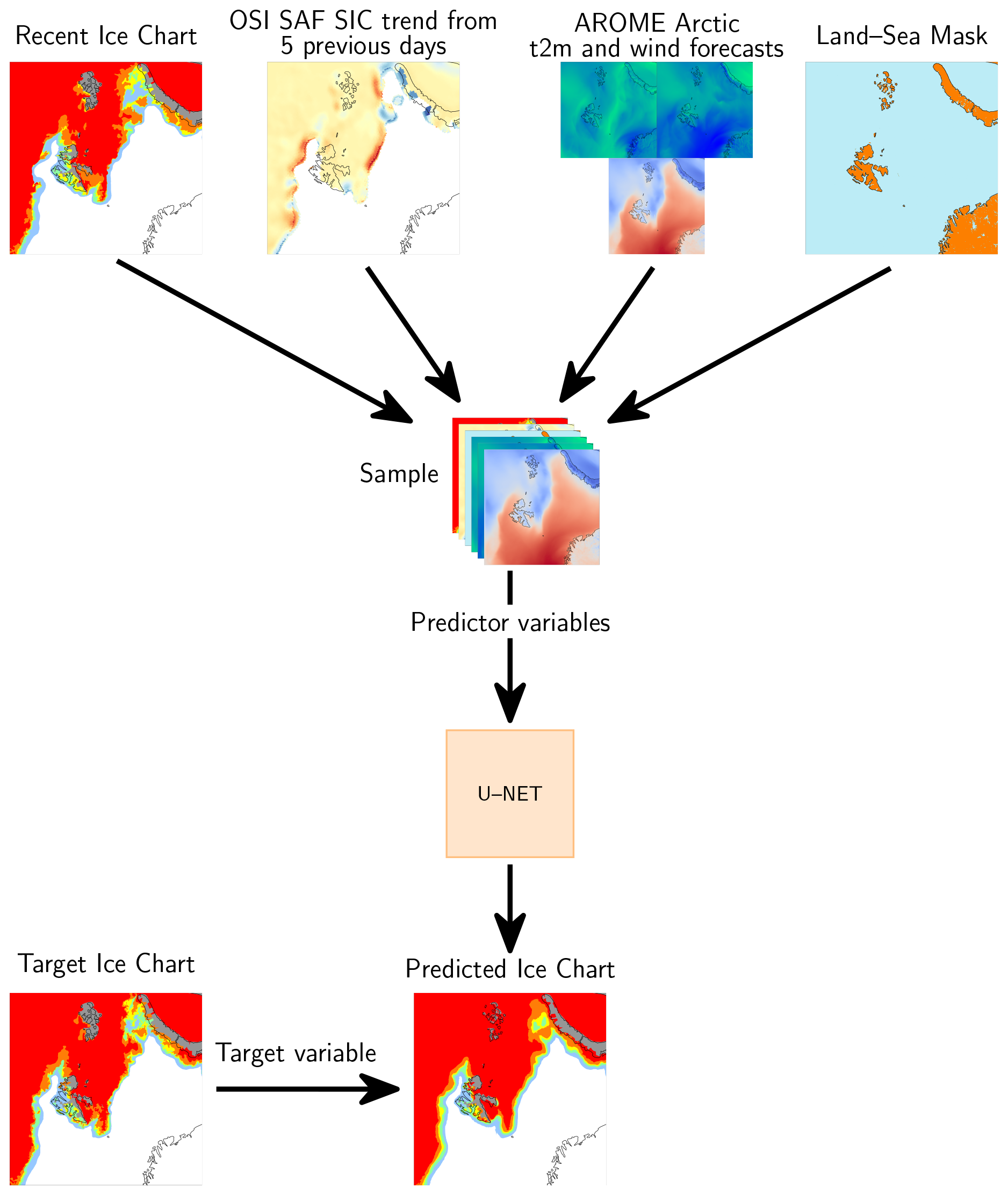
Figure 3 Overview of the input and output to the deep learning forecasting system. The predictors are constructed from individually preprocessed sources and are provided to the network together with an associated target ice chart.

3.4 Verification metrics

We chose to focus on skill metrics based on sea ice edges when validating the performance of the deep learning forecasts as such metrics are appropriate when the SIC is discretized as categorical contours. These metrics are also relevant for end users (Melsom et al., 2019; Fritzner et al., 2020; Wagner et al., 2020). Specifically, we derive the length of the sea ice edge following the method introduced in Melsom et al. (2019) and assess forecast skill using the integrated ice edge error (IIEE) (Goessling et al., 2016) normalized with the ice edge (or threshold SIC contour) length derived from the target SIC field (nIIEE). The nIIEE is chosen since it is not particularly affected by isolated ice patches (Palerme et al., 2019). Moreover, the nIIEE, when normalized according to a SIC contour length, is independent of the sea ice seasonality (Goessling et al., 2016; Palerme et al., 2019; Zampieri et al., 2019), which allows for a comparison of forecast skill across seasons. Finally, the nIIEE can be interpreted as the SIC contour displacement error between two products, which is easy to interpret and relevant to end users (Melsom et al., 2019). To the best of the authors' knowledge, the nIIEE has only been assessed using coarse-resolution sea ice concentration fields. However, we compared the nIIEE computed from ice charts at 1 km spatial resolution and 10 km resolution between 2019–2022 and found the Pearson correlation to be 0.98, which ensures the validity of also applying nIIEE to high-resolution SIC. For further details, see the Appendix.

3.5 Baseline forecasts

We compare the deep learning forecasts against three baseline forecasts: the persistence of the observations, the linear trend in sea ice concentration from OSI SAF SSMIS, and a purely wind-derived sea ice motion estimation based on free drift. The baseline forecasts serve as a lower threshold which the deep learning system must outperform in terms of nIIEE in order to be considered skilful. A persistence forecast involves keeping the initial state of the system constant in time. The baseline forecast based on the linear trend is created by computing a pixelwise linear trend from the previous 5 d, which is used to advance the system forward in time. For clarity, the computed values are bounded to match the valid value range [0,100]. The use of a linear SIC trend as a baseline forecast has previously been assessed in Grigoryev et al. (2022), where the authors reported that the linear trend consistently achieved a higher mean absolute error than persistence.

The wind-driven free-drift baseline forecast is implemented following the description in Zhang et al. (2024). Hence, sea ice motion is estimated to be 2 % of the surface wind speed 20° to the right (clockwise) of the surface wind direction. New positions are calculated by advecting each grid cell with its corresponding wind speed using a first-order forward Euler integration scheme. Since the free-drift forecast advects sea ice parcels individually based on limited-area wind forcing, the free-drift forecast is not guaranteed to be spatially consistent as some grid cells might not be covered by sea ice after advection, while they are clearly in the sea ice pack. Thus, we perform nearest neighbour interpolation after advecting the sea ice to ensure that the free-drift forecasts are spatially consistent. Additionally, it is described in Germann and Isztar (2002) that simple advection schemes tend to introduce numerical diffusion, resulting in a loss of smaller-scale features. Finally, in order to be consistent with the deep learning models, input SIC is advected with the same AROME Arctic mean surface wind fields also supplied as predictors to the deep learning model.

3.6 Model intercomparison setup

The goal of the model intercomparison is to assess the predictive skill of the deep learning forecasts against the described baseline forecasts and physical forecasting system. In order to compare the different sea ice forecasts, all products were projected and interpolated onto the grid of the coarsest-resolution product, which is neXtSIM (3 km) or AMSR2 (6.25 km), depending on which SIC product is used for evaluation. The baseline forecasts have a daily output frequency that is similar to that of the deep learning system; hence the comparison involves identifying the forecast with similar start and target dates. However, both Barents-2.5 and neXtSIM forecasts have an hourly frequency. When comparing the deep learning forecasts against both physical models, we use the physical forecasts initiated at 00:00 UTC the day following deep learning initialization. Furthermore, physical models are averaged between 00:00 and 12:00 UTC on the target date of the deep learning forecast due to the ice chart production process. This setup is assumed to moderate spatial variability induced by the lack of a temporal mean.

4 Results

4.1 Training performance and data considerations

Training the deep learning system for 25 epochs takes approximately 3 h 30 min on the A100 GPU, whereas performing a single prediction takes 6 s on a workstation CPU (AMD EPYC 7282 16 core) and 30 s on a laptop CPU (Intel^® Core™ i7-8565U 8 core). Comparatively, a single member of Barents completes a 24 h forecast in ≈12 min, resulting in a 99 % speed-up when running on comparable hardware. The optimal U-Net width of 256 channels in the bottleneck was determined by performing a grid search on the validation dataset across the learning rate (0.0001–0.01) and U-Net bottleneck width (256–1024) (see Fig. S2 in the Supplement). To achieve consistent architectures between the developed models, we considered only variations in the 2 d target lead time model for the grid search and reused the results for models targeting all lead times. The final model contains 2.4 ×10⁶ trainable parameters, with 1.15 ×10⁶ of these being located in the encoder and 1.25 ×10⁶ in the decoder. We compared model implementations without cumulative contours (single output, multi-class segmentation with categorical cross-entropy loss) against deep learning models reformulated with cumulative contours, and we obtained a better preservation of intermediate contours with the model predicting cumulative contours, especially at longer lead times (see the Supplement). Figure 4 presents a forecast from a deep learning model with cumulative contours targeting 2 d lead time and shows that intermediate SIC categories have been resolved in the forecast. For the example presented in Fig. 4, the deep learning forecast achieved an nIIEE of 7.5 km, while persistence achieved an nIIEE of 13.4 km. We observe in Fig. 4 that the deep learning forecast is able to reproduce the SIC increase in the Barents Sea and the reduction in a polynya area north-east of Svalbard. An apparent difference between the deep learning forecast and the ice charts is that the different contours include less structural details in the deep learning forecasts, which results in a smoother appearance.

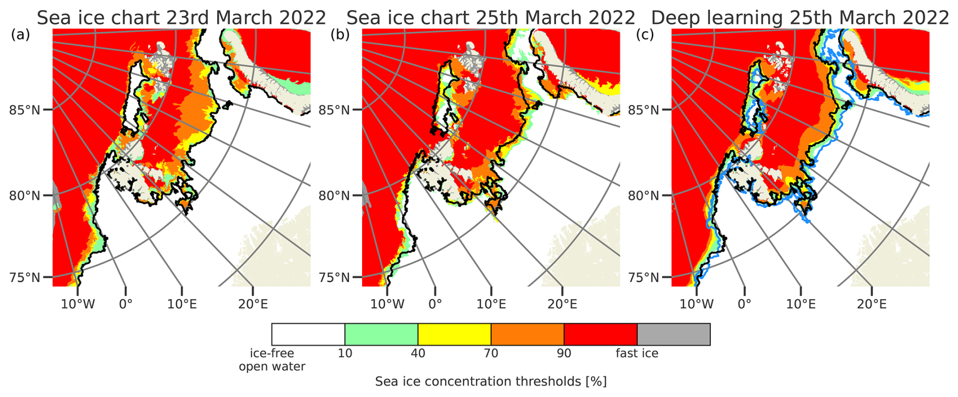
Figure 4 Ice charts for (a) 23 and (b) 25 March 2022, with a deep learning prediction for 25 March 2022 initialized on 23 March 2022 in (c). The black line is the sea ice edge for the ice chart in (a), and the blue line is the sea ice edge for the ice chart in (b), both plotted for a 10 % concentration threshold. The <10 % SIC category is not shown.

Figure 5 compares the ability of the deep learning system to resolve sea ice categories against ice charts and AMSR2 observations. In general, the deep learning system accurately resolves the concentration category distribution in accordance with the ice charts, regardless of lead time, with all categories being less than 1 % different from the ice chart distribution when considering the yearly average. When comparing against the AMSR2 observations, it is important to note the differences in the occurrence frequency of the 100 % SIC category. The ice charts consider fast ice a separate category representing land fast ice, which is a distinction not made by the ASI retrieval algorithm, although, for consistency, 100 % SIC from AMSR2 has been regarded as fast ice for this study. However, the normalized integrated ice edge error only considers the lower boundary of any concentration category, and, as such, this choice does not affect the results from the nIIEE skill score. This choice is reflected in Fig. 5, where the resolved fraction of very close drift ice is 20 % in AMSR2 compared to 31 % in the ice charts. Comparatively, the fraction of resolved fast ice in AMSR2 is 8 %, whereas this category constitutes <1 % of the area for the ice charts.

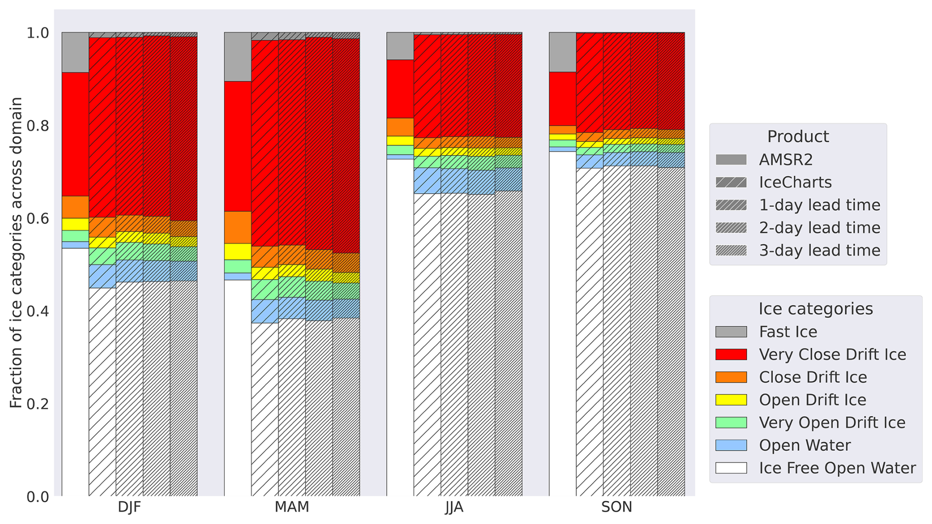
Figure 5 Seasonal distribution of each SIC category for 2022 as the respective fraction of the total mean SIC area for AMSR2, ice charts, and the deep learning system at 1–3 d lead time. The AMSR2 data have been projected onto the deep learning model domain.

Another difference between AMSR2 observations and the ice charts presented in Fig. 5 is how ice-free open water and open water are resolved. On a yearly average, ice-free open water constitutes about 62 % of the AMSR2 pixels and 55 % for the ice charts. Furthermore, open water is represented more in the ice charts, constituting about 5 % of the pixels, while for the AMSR2 observations, this category covers only 1 %. This is because the ice charts consider SAR and optical satellite retrievals with a higher sensitivity to low ice concentrations to resolve open water compared to passive microwave sensors, which have a low sensitivity to SIC below 15 %.

4.2 Forecast performance and model intercomparison

We initially compare the deep learning forecasts against the baseline and dynamical forecasts in 2022 across all target lead times, where we consider the yearly mean of the nIIEE for different sea ice edge contours defined by (10 %, 40 %, 70 %, and 90 %) concentration thresholds in Fig. 6. For all considered lead times and concentration thresholds, the deep learning forecasts achieve the lowest nIIEE. Similar to persistence, nIIEE for the deep learning forecasts increases proportionally with lead time, although at a lower rate. Additionally, the neXtSIM, free-drift, and linear trend forecasts are not able to outperform persistence on average for the 10 % concentration contour, scoring factors of 1.57, 1.12, and 1.34 higher than persistence, respectively. Furthermore, the mean nIIEE between forecasts based on ice charts (deep learning, persistence, and free drift) and neXtSIM and the linear trend, which are forced by a different sea ice concentration source, is notably shifted from the 70 % concentration thresholds and above. However, we also trained deep learning models on input AMSR2 passive microwave observations with ice charts as the target, and the deep learning predictions retained sufficient skill comparable to ice chart persistence while achieving somewhat higher nIIEE than deep learning models trained on input ice charts (see the Supplement).

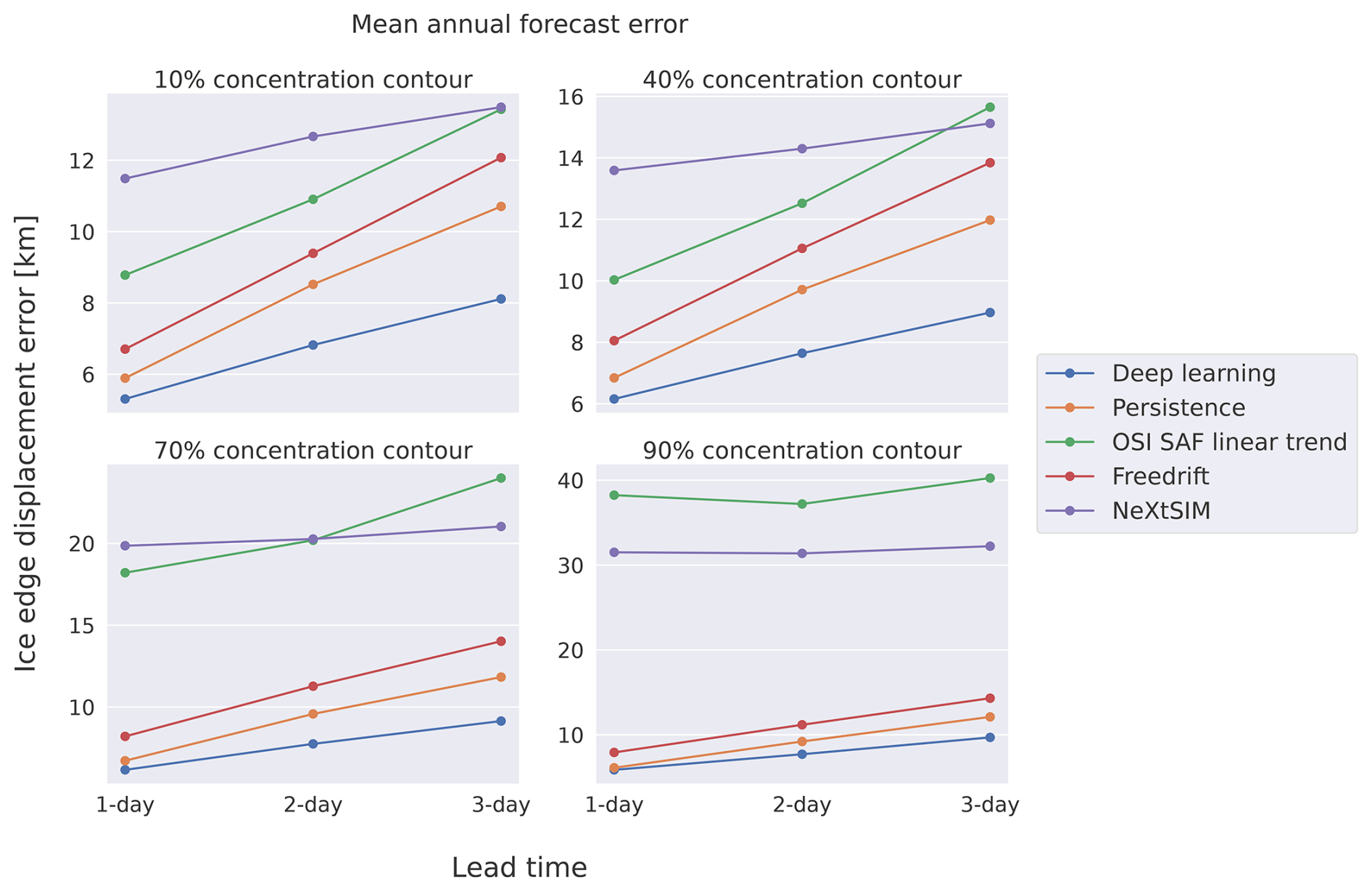
Figure 6 Mean annual ice edge displacement error as a function of lead time for different sea ice concentration contours defined by 10 %, 40 %, 70 %, and 90 % SIC. Only products with complete coverage of 2022 have been considered. Ice charts are used as a reference product.

The deep learning forecasts improve upon persistence by reducing the nIIEE_10 % by a factor of 0.82. In terms of error growth as a function of lead time, the linear trend forecast is the only forecast where the slope of the error increases with increasing lead time, regardless of concentration threshold. This indicates that the linear trend from past OSI SAF SSMIS observations is unable to capture ice chart evolution, especially for longer lead times. Moreover, although neXtSIM forecasts have a comparatively high nIIEE initially, the error growth with lead time is the lowest for all concentrations, indicating that neXtSIM may provide more useful forecasts at longer lead times, especially for lower concentrations.

Figure 7 shows how the deep learning system resolves the seasonal variation in the sea ice edge length for different lead times. The predicted sea ice edge follows a similar seasonal pattern to that of the ice edge length from the target ice charts. Each monthly mean predicted sea ice edge length has a negative bias compared to the ice charts, which increases for longer lead times. Given that the deep learning forecasts resolve the different categories akin to the ice charts, we attribute the apparent negative bias of the length to the lack of details along the forecast contour edges. Hence, the SIC contour smoothness is somewhat proportional to forecast lead time.

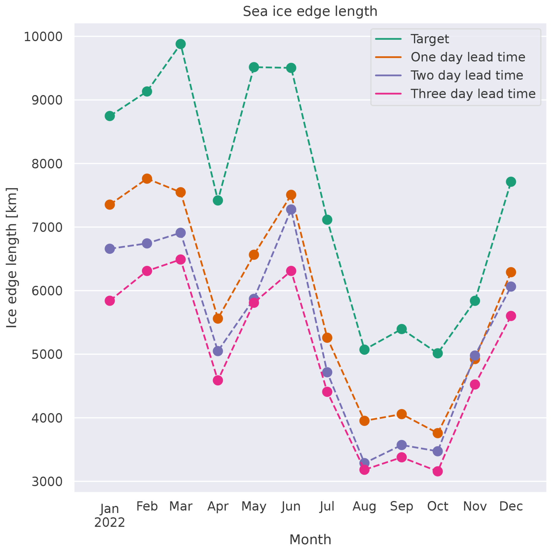
Figure 7 Mean monthly sea ice edge length for 2022, with the sea ice edge defined by a 10 % concentration threshold. The considered products are the ice charts and deep learning system for 1–3 d lead times.

In order to assess the consistency of the deep learning forecasts trained on ice charts, we evaluate the performance by replacing the ice charts with AMSR2 observations as the reference dataset in Fig. 8. When utilizing AMSR2 observations as a reference, the number of samples used to evaluate the forecasts is consistently 247 across all lead times. We see in Fig. 8 that the deep learning forecasts on average achieve the highest nIIEE when considering a 10 % concentration contour, achieving a mean nIIEE_10 % of 16.7 km across the lead times. The displacement is consistent with the inherent nIIEE difference between the AMSR2 observations and the ice charts (Fig. 5), which we found to be 13.3 km for the 10 % concentration contour when compared across the test dataset. Furthermore, AMSR2 persistence forecasts achieve the lowest nIIEE on average for the same contour. When considering SIC contours defined by ≥40 % SIC, the deep learning forecasts perform closer to AMSR2 persistence, although they achieve a slightly higher nIIEE on average. neXtSIM on average outperforms the deep learning forecasts for the 10 % concentration contour; however this is not the case for the 40 %, 70 %, and 90 % concentration contours, where the performance is close to the initial error for all lead times, similar to the behaviour shown in Fig. 6. For the contours higher than 10 % SIC, Fig. 8 shows that the AMSR2 persistence, AMSR2 free-drift, and deep learning forecasts on average gradually improve against both neXtSIM and the linear trend, with the deep learning forecast increasing its improvement against neXtSIM for higher contours. The difference between AMSR2 free drift and AMSR2 persistence can also be seen to decrease for increasing concentration contours, yet AMSR2 free drift achieves a higher nIIEE than the AMSR2 linear trend considering the 10 % and 40 % concentration contours. Overall, AMSR2 persistence mostly achieves the lowest nIIEE, although it is surpassed by the deep learning forecasts when higher concentration contours (≥90 %) and ≥2 d lead time are considered. Moreover, the deep learning forecasts achieve the lowest nIIEE scores when predicting the 40 % concentration contour from the AMSR2 observations, in good agreement with the average nIIEE difference between AMSR2 and the ice charts, which we found to be 9.7 km for the same concentration contour.

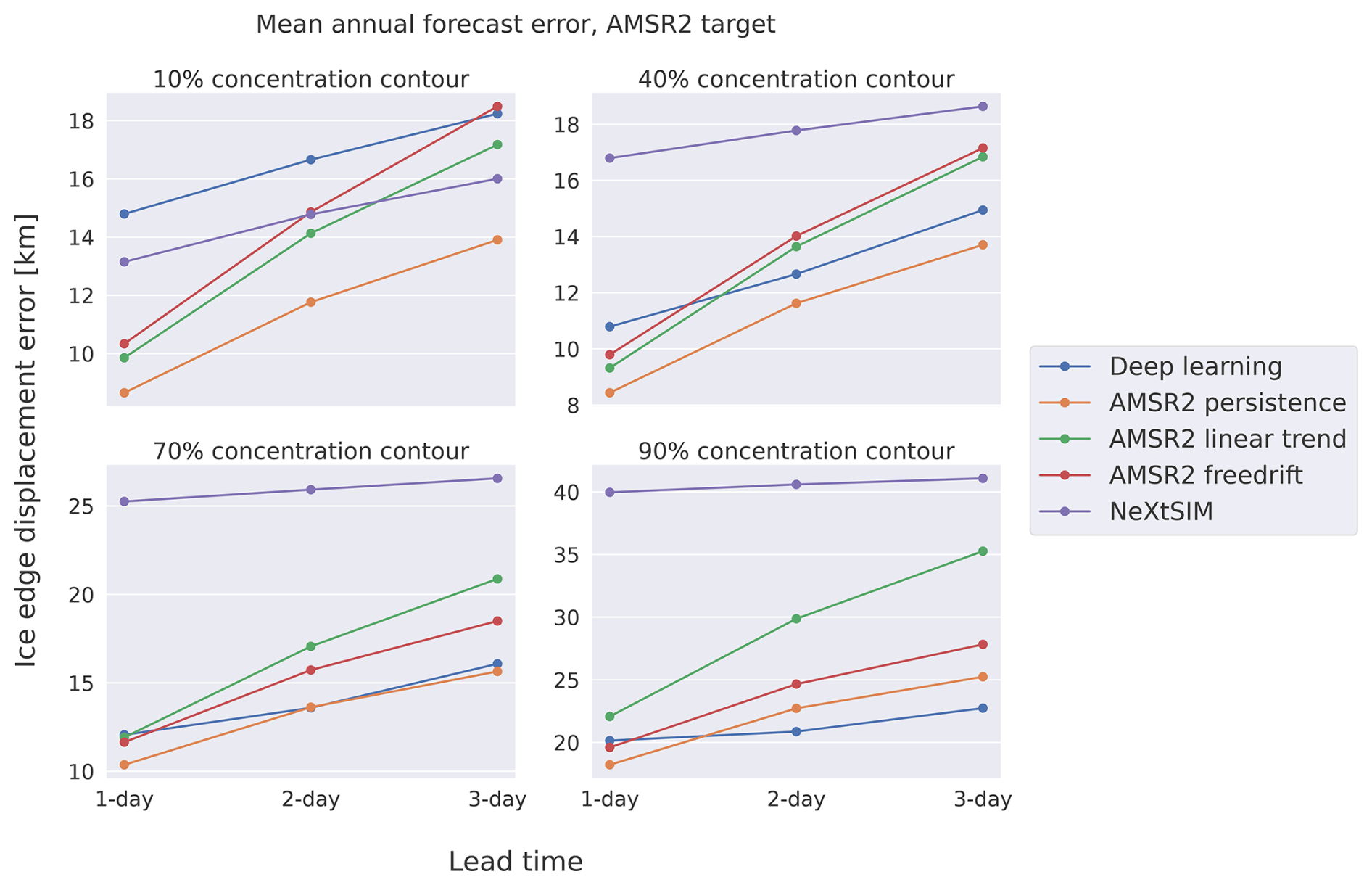
Figure 8 Mean annual ice edge displacement error as a function of lead time. The ice edge displacement error for the different products has been computed considering AMSR2 observations as reference.

The model intercomparison experiment, which compares the deep learning system against baseline and dynamical sea ice forecasts for all seasons, is presented in Fig. 9 using the ice charts as reference. For all considered lead times and target contours, the deep learning forecasts achieve the lowest seasonal mean nIIEE. The seasonal axis of Fig. 9 shows that the ice chart persistence, free-drift, and deep learning forecasts all achieve higher nIIEE values during winter and spring, associating the errors with the periods of freeze-up and sea ice maximum extent. When the nIIEE is computed from the 70 % or 90 % concentration contours, Fig. 9 shows that the forecasts not utilizing ice chart information (i.e. linear trend, neXtSIM, and Barents-2.5) attain considerably higher values, especially during summer. This pattern might indicate a discrepancy between the ice charts, the dynamical forecasts, and the linear trend with regard to how higher SIC is resolved, further influenced by seasonal conditions.

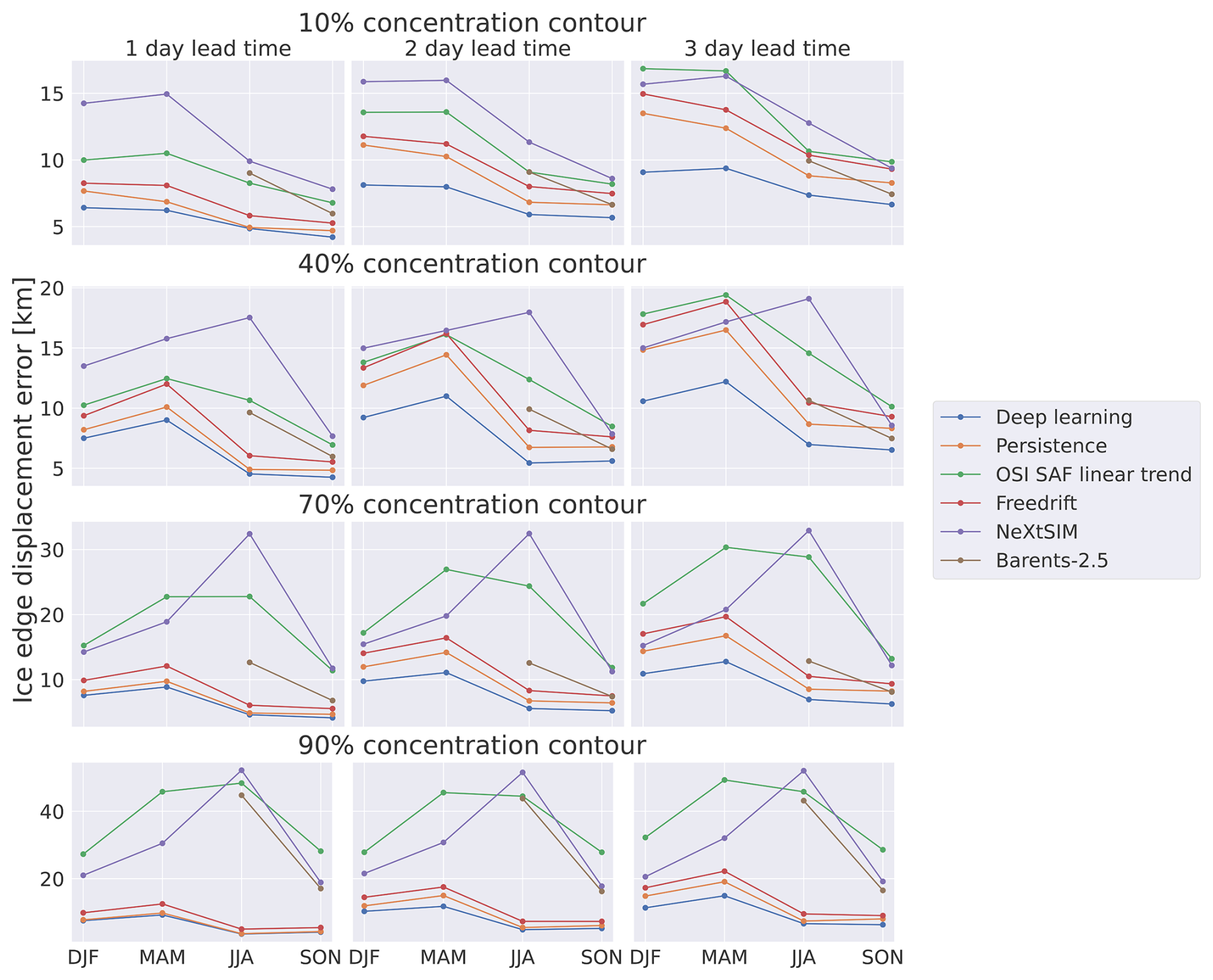
Figure 9 Model intercomparison for varying seasons, lead times, and concentration contours. The ice charts are regarded as the reference. The values reported represent the integrated ice edge error normalized according to the length of the current SIC contour from the reference ice chart in kilometres. The OSI SAF linear trend is computed from the past 5 d. Barents-2.5 results are only shown for summer and autumn.

4.3 Feature importance

To better understand the importance of the different predictors used, as well as the sensitivity of the deep learning system to the predictors, we measured how the model responds to modified predictors. In order to measure the impact of each predictor, we first conducted an experiment where the nIIEE was computed from deep learning models fitted to different predictor subsets. The effect of including different predictors on deep learning forecast performance is shown in Fig. 10. In general, removing predictors tends to decrease the predictive skill of the deep learning system, except for 2 m temperature for 2 d lead time and the past trend for 3 d lead time. Removing the current ice chart has the highest impact on performance (mean +7.14 km on average for all lead times), reducing the skill of the model below that of persistence. However, the impact of removing ice charts is reduced for increasing lead times. Contrarily, the loss of skill associated with removing all AROME Arctic predictors increases with lead time. Although no other combination of withheld predictors decreases the skill of the deep learning forecasts below persistence, removing all atmospheric forecasts has a consistent negative impact on forecast skill (+1.31 km on average) – more than any other removed set – except SIC from ice charts. Comparing the impact of the different predictors originating from AROME Arctic shows that removing both wind components simultaneously has a greater effect on forecast skill (+0.86 km) on average than removing 2 m temperature (+0.08 km). Models trained without the past sea ice trend perform comparably to default deep learning models (+0.06 km).

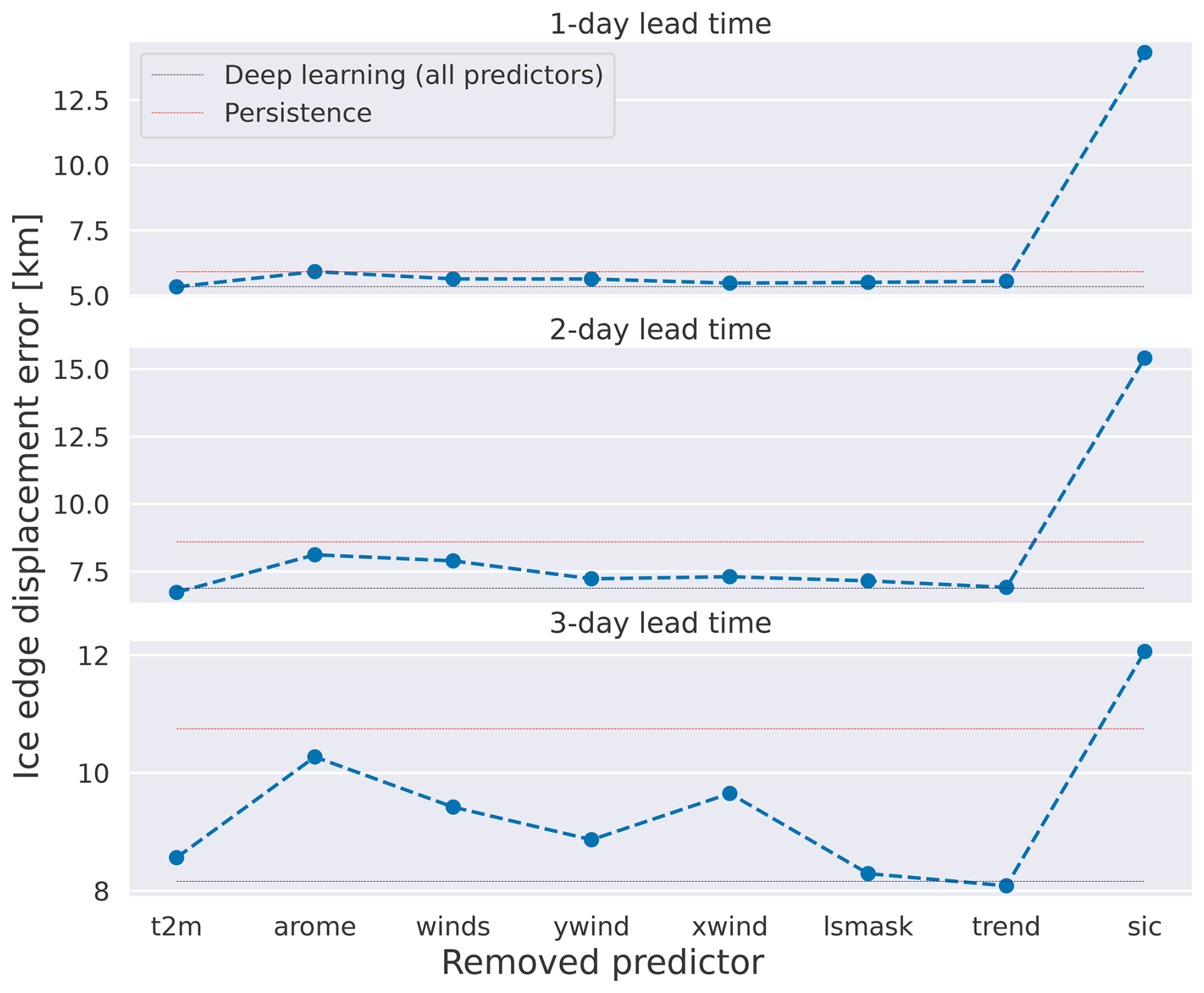
Figure 10 Yearly mean nIIEE when a subset of the predictors is withheld during training. The dashed black line denotes yearly mean nIIEE for deep learning forecasts from a model with all predictors, and the dashed red line denotes the skill of persistence. AROME refers to the removal of all atmospheric predictors during training. Winds are similar except for the two wind components.

We also conducted a permutation feature importance analysis to quantify the importance of each predictor for a deep learning model trained on all predictors. Permutation feature importance involves randomly shuffling the input sequence of a single predictor and analysing how much this alters the predictive skill of the model. To minimize the potential impact of a seasonal cycle appearing in the reordered predictors, the experiment was run 10 times for each predictor. Permutation feature importance is model-specific and does not provide insight into the predictive capabilities of the analysed predictors. Figure 11 shows the predictor importance evolution over increasing lead times as the difference in the ice edge displacement error from the reference deep learning forecasts. Although the importance of each predictor varies with lead time, the order of importance is consistent between all lead times, with the recent ice chart being the most important predictor, near-surface temperature ranking second, and – finally – the two wind components ranking approximately equal as the third-most important predictors. Only permuted ice charts and near-surface temperature significantly decrease the deep learning forecast score below the benchmark skill of persistence. Only ice charts and 2 m temperature at 3 d lead time attained a noticeable standard deviation (≥0.1 km) from inputting predictors from different dates. There is an inversely proportional relationship between the importance of the recent ice chart (decreasing) and the importance of the atmospheric forecasts (increasing) when targeting longer lead times, indicating that the model is more reliant on the future state of the predicted system (atmospheric forecasts) rather than the initial state (recent ice chart) for longer lead times. Hence, Fig. 11 suggests the existence of a limit to the predictive capability gained from providing only current sea ice conditions, similar to how persistence and linear trend forecasts inherently lose skill at longer lead times. The skill difference from past sea ice information encoded in the OSI SAF linear trend is indistinguishable (+0.01 km) from the performance of non-permuted deep learning forecasts; hence the deep learning forecasts are not dependent on the past state of sea ice, regardless of target lead time.

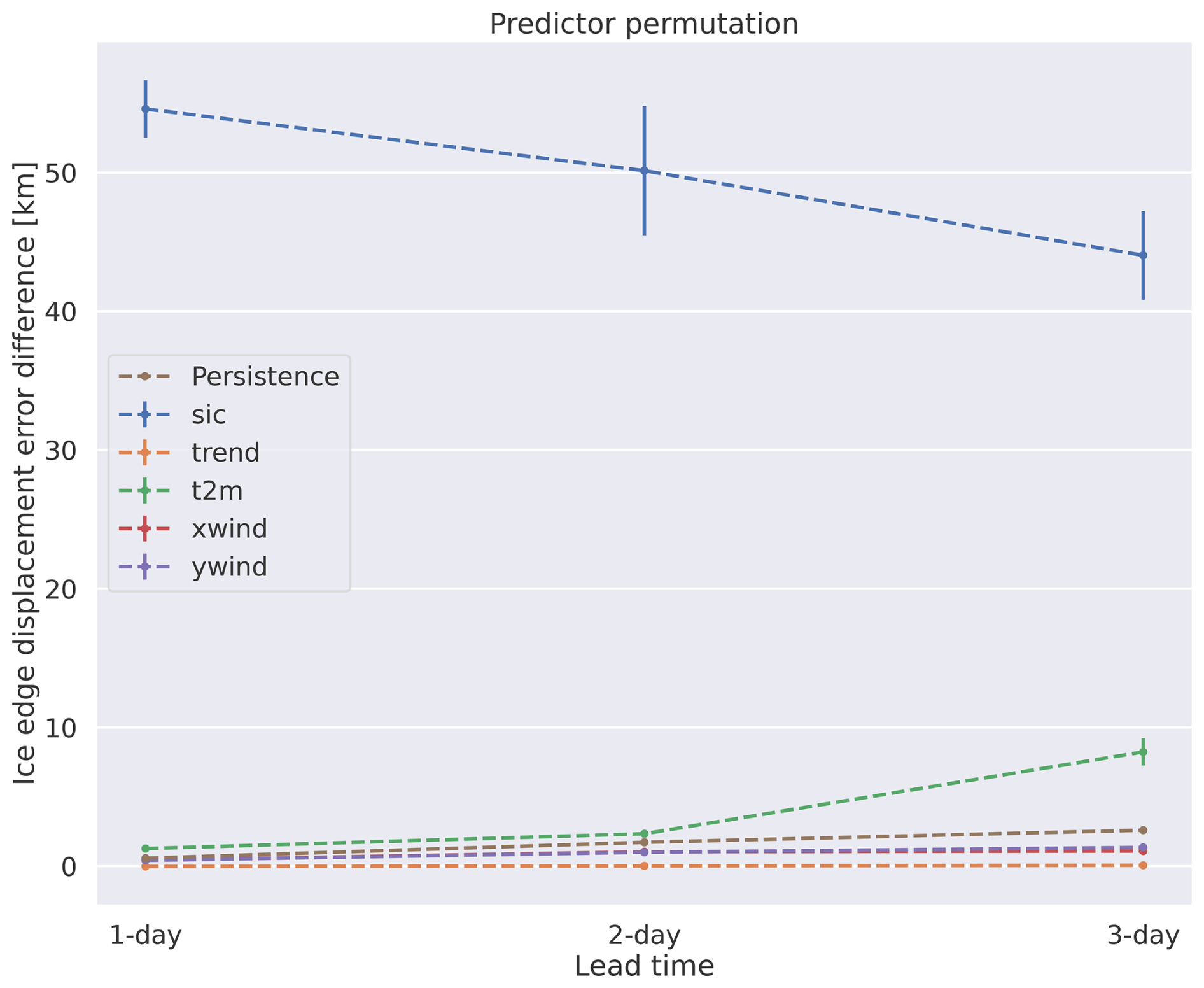
Figure 11 Yearly mean nIIEE where the sequence of a predictor in the test dataset has been shuffled, repeated 10 times for all predictors. Each line represents a permuted predictor sequence. Unaltered persistence forecasts are included as benchmark references. The land–sea mask predictor was excluded from the analysis as it is static regardless of the forecast start date.

5 Discussion and conclusions

This study presents the development of a deep learning forecasting system targeting high resolution (1 km) and short lead times (1–3 d), taking into account operational constraints related to the real-time availability of data. In order to adequately resolve the skewed distribution of SIC classes in the ice charts (especially in the MIZ, which is crucial for skilful forecasts, ensuring maritime safety; Wagner et al., 2020), we present a novel reformulation of the target data and decoder from the original U-Net architecture of Ronneberger et al. (2015), which we refer to as cumulative contours (Eq. 1). The cumulative contours demonstrate how combining architectural design from multi-task learning (Zhang et al., 2014) with task-specific additive properties of SIC intervals positively benefits deep learning forecasting skill, especially with respect to resolving the intermediate SIC intervals constituting the MIZ. With this reformulation of U-Net, the deep learning forecasts are able to consistently outperform the baseline forecasts and operational short-range dynamical sea ice forecasting systems (neXtSIM-F and Barents-2.5) in terms of achieving the lowest ice edge displacement error when considering the ice charts as reference.

Despite training deep learning models to predict SIC conditions from the ice charts only, the deep learning forecasts behave similarly to baseline forecasts when validated against independent AMSR2 SIC observations (Spreen et al., 2008) for concentration contours of ≥40 %. The increase in deep learning performance seen between the 10 % and 40 % concentration contours may be indicative of a shift in SIC distribution for lower concentration values between the two products, as further indicated by the increased similarity in occurrence frequency between AMSR2 and the ice charts when considering open and closed drift ice reported in Fig. 5. It is noted that the ASI sea ice retrieval algorithm exerts larger uncertainties for lower concentrations (Spreen et al., 2008), whereas SIC<10 % is visible in SAR and optical satellite images used by ice analysts drawing ice charts. However, ice charts are influenced by human decision-making, especially in the medium concentrations (40 %–70 %) of the MIZ (Dinessen et al., 2020), which may be a source of ice edge location discrepancy between the two products. The overall performance – regardless of reference product – suggests a degree of consistency in the developed forecasts between the two reference products. However, the analysis also suggests that inherent differences between sea ice products are reflected by deep learning forecasts, and we can not expect the forecasts to improve beyond that initial difference as the models are trained to only minimize the statistical error of their target sea ice product.

The results from the forecast intercomparison analysis demonstrate that the deep learning forecasts meet the requirements for forecast accuracy while considerably reducing computing time. However, the results from the analysis could be influenced by the uneven sample sizes used for verification at different lead times. Hence, we recommend evaluating the forecasts with longer time series when they become available. With respect to the development of the operational weather prediction system AROME Arctic, a continued forecast evaluation can also facilitate the understanding of model response to continuously updated atmospheric predictors and the potential of fine-tuning deep learning models. With regard to operationalization, the input data supplied to the deep learning forecasting system have been chosen with consideration of publishing time, with a special constraint for AROME Arctic being the 66 h forecast length. The current setup allows 3 d forecasts to be published every weekday and to be sent to maritime operators in advance of their valid date, covering Saturdays and Sundays when Norwegian ice charts are not produced.

The predictor importance analysis suggests that the deep learning models benefit from an increased and diversified dataset by increasing the precision of the predicted sea ice edge by 1.31 km when atmospheric forecasts from AROME Arctic (Müller et al., 2017) are included as predictors. The inclusion of forecast predictors from weather forecasts has previously been shown to increase predictive skill (Grigoryev et al., 2022; Palerme et al., 2024), which further motivates the inclusion of other forecasted physical forcings affecting sea ice as predictors. We recommend further work to investigate currently unexplored metocean forcings, such as ice–wave interactions (Williams et al., 2013), by including fields such as forecasted wave height and wave direction. However, expanding the dataset towards past temporal regimes by including a coarse-resolution linear SIC trend derived from OSI SAF observations was shown to have a marginal effect on the forecast skill, indicating that the deep learning models were unable to infer sea ice growth/decline from past observations (Fig. 11), in line with the results of Palerme et al. (2024).

When all predictors were provided as inputs to the deep learning models, the skill of the forecasts was particularly sensitive to the initialization date of the inputted ice chart (Fig. 11). This suggests that a large part of the inferred physics and seasonality originates from the ice charts, which can also explain why the atmospheric predictors were not essential to outperform persistence. Additionally, the comparison made against free-drift SIC forecasts suggests that the deep learning model has learned a relationship between the input predictors and target ice chart that is beyond a sea ice motion estimation linearly proportional to the near-surface winds. Although it is unknown how the deep learning model responds to individual predictors, the comparison suggests that the model's ability to learn non-linear relationships in the input data helps in predicting SIC. Moreover, the comparison suggests that inferring thermodynamical properties that allow the model to grow and melt sea ice aids in predicting short-term SIC beyond that of advection.

When considering the initialization time of the AROME Arctic predictors, the lessened impact of the atmospheric predictors could also be associated with AROME Arctic not covering the beginning of the forecast period, especially for shorter lead times. Nevertheless, as the model's sensitivity to the current ice chart tends to decrease for longer lead times, understanding how the model utilizes the increasingly important forecast predictors should be considered, especially when targeting longer lead times. Other works have investigated the use of explainable artificial intelligence methodologies for interpreting climate-science deep neural network models and results (e.g. Toms et al., 2020; Ebert-Uphoff and Hilburn, 2020; Bommer et al., 2023). This should be given more attention as they present an opportunity to develop new tools for diagnosing machine learning sea ice forecasting systems.

Appendix A: Comparing nIIEE for high- and low-resolution sea ice concentration

In order to evaluate 1 km resolution sea ice forecasts using the ice edge displacement error as derived by Melsom et al. (2019), we assess the validity of applying the metric to high-resolution sea ice forecasts by comparing it against a coarse-resolution (10 km) reference case. We compute nIIEE from the ice charts at 2 d lead time persistence, with ice charts at 1 km resolution and downsampled onto a 10 km grid covering the period 2019–2020. Mean monthly nIIEE for both forecasts is shown in Fig. A1. The correlation coefficient between both nIIEE curves in Fig. A1 is 0.98. The strong correlation indicates that the nIIEE is preserved when used in a 1 km resolution environment.

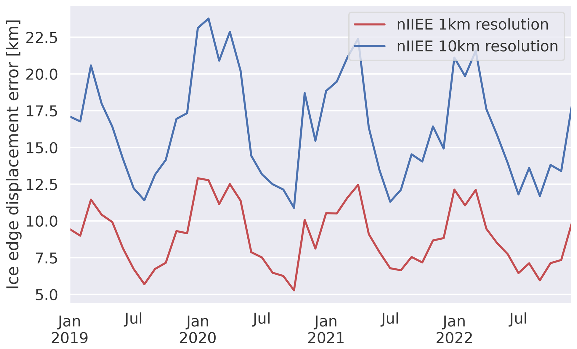
Figure A1 The nIIEE computed across the entirety of the training dataset (2019–2022) for 2 d lead time ice chart persistence with the ice charts as reference. The sea ice edge length used to divide the computed IIEE was derived from the same resolution as the respective forecast.