Comparing high-resolution snow mapping approaches in palsa mires: UAS lidar vs. modelling

Snow cover has an important role in permafrost processes and dynamics, creating cooling and warming systems and impacting the aggradation and degradation of frozen soil. Despite theoretical, experimental and remote-sensing-based research, a comprehensive understanding of small-scale snow distribution at palsas remains limited. In this study, we used unoccupied aerial systems (UASs) equipped with light detection and ranging (lidar) to generate high-resolution digital terrain models (DTMs) and derive spatially continuous snow depth maps over palsa mires in northwestern Finland. For the first time, snow distribution was recorded over a palsa using UAS lidar. The resulting snow depth maps showed sufficient accuracy, with a root-mean-square error (RMSE) of 23.49 cm and an R² value of 0.691 when compared to in situ measured snow depth validation data. To enhance the interpretation of snow distribution patterns, we applied a random forest (RF) machine learning model trained with in situ snow depth measurements and terrain parameters derived from the UAS lidar DTMs. This approach resulted in improved accuracy, with an RMSE of 18.33 cm and an R² value of 0.77. RF performs particularly well when modelling snow distribution over thermokarst and vegetated areas, demonstrating the potential of machine learning to capture small-scale patterns based on field observations. The UAS lidar also enables a very detailed analysis of the interactions between snow and permafrost. Both approaches reveal snow accumulation zones, especially at steep palsa margins and within cracks, where insulation limits frost penetration and contributes to degradation processes such as block erosion. In contrast, a thinner snow depth on exposed palsa surfaces allows deeper frost penetration, which initially stabilizes the ice core but then leads to the formation of steep edges and further degradation.

1 Introduction

Snow cover plays an important role in permafrost processes and dynamics. Its physical characteristics impact the aggradation and degradation of frozen soil (Barry, 2002). In March 2023, around 39.26×10⁶ km² of the Northern Hemisphere was permanently or partly covered with snow (NOAA, 2023), affecting around 14.77×10⁶ km² of permafrost area (Ran et al., 2022). This includes the discontinuous permafrost areas in the northern parts of Sweden, Norway and Finland, known as Fennoscandia. Due to changes in climate, a reduction in snow cover duration is expected (Quante et al., 2021), leading to changes in air and soil temperature interactions and resulting in negative impacts on permafrost soils (Chen et al., 2021). This has a direct impact on ecological processes, such as the reduced albedo in winter that leads to higher energy uptake by soils (Thackeray and Fletcher, 2016) and longer growing seasons (Madani et al., 2023). In addition, Wang et al. (2024) showed that snow cover – in combination with landscape heterogeneity – plays an important role in controlling soil temperatures throughout the year. The Intergovernmental Panel on Climate Change (IPCC) already highlighted in their latest report that the loss of permafrost within this century is expected in these regions (IPCC, 2023). In northern Fennoscandia, particularly in northern Finnish Lapland – the main focus of this study – specific periglacial permafrost landforms known as palsas are at risk of disappearing within this century (Leppiniemi et al., 2023).

The occurrence of palsas, small mounds up to 4–7 m in height with a frozen core, is bound mainly to the presence of peatlands and is driven by climatic parameters (Meier, 2015; Seppälä, 2011). Palsas serve as indicators of climate warming, as their degradation and disappearance reflect rising temperatures (Leppiniemi et al., 2023). Additionally, they provide important habitats for various animal species (Luoto et al., 2004) and hold significant cultural and societal value for indigenous and local communities, particularly in the context of traditional reindeer herding (Markkula et al., 2019). Given their ecological and cultural importance, monitoring their changes is essential. Palsas are highly sensitive to temperature insulation shifts induced by snow during winter. Their development is directly influenced by variations in snow depth, which regulate thermal insulation in winter and protect against warm air and sunlight in spring, ultimately affecting active layer thickness (ALT) and soil warming (Park et al., 2015; Verdonen et al., 2023, 2024). In winter, deep snow cover insulates the ground, reducing the penetration of cold temperatures and keeping the underlying soil comparatively warmer. In summer, this accumulated snow delays ground warming and slows permafrost thawing, resulting in a shallower ALT. These areas are defined as warming areas throughout this article. They are typically found in depressions, concave terrain or wind-sheltered locations where snowdrifts accumulate. Conversely, thin snow cover allows for more intensive winter cooling due to reduced insulation, leading to greater heat loss from the ground. In summer, these areas warm up earlier, causing a deeper ALT. Such locations are defined as cooling areas. They are commonly found in elevated or wind-exposed areas of the palsa, where snow accumulation is naturally limited (Seppälä, 1982; Olvmo et al., 2020). This influence on palsas was empirically demonstrated by Seppälä (2011), who described the impact of variable snow cover on palsa thermal dynamics during subsequent thawing periods. Moreover, experiments show that the depth of snow cover mainly influences the development of palsas (Seppälä, 1982). Deviations from the usual thickness of snow cover, whether thinner or thicker, induce varying changes in palsa dynamics. For example, at the steep edges of palsas, the accumulation of snow can pose a risk, destabilizing the frozen core due to increased thermal insulation at these specific areas and leading to a higher risk of block erosion (Olvmo et al., 2020; Seppälä, 1994). Despite theoretical, experimental and remote-sensing-based research, a comprehensive understanding of actual snow distribution conditions within and around palsas remains limited (Seppälä, 2011; Verdonen et al., 2023). Although they have high potential for accurate mapping, unoccupied aerial systems (UASs) have not yet been used to measure snow depth in palsa mires.

Consequently, detailed data on snow distribution in palsa mires are not available. Even if sufficient climate data are made available through official weather stations, the microclimate inside these mires impacts the snow distribution in various ways, especially as relates to snow drifts due to strong winds, as monitored by Zuidhoff (2002). Since palsa mires occur mostly in remote areas, simple interpolation of climatic observations from weather stations within the same region does not provide data on the actual state within these mire complexes, which does not allow for monitoring the exact snow distribution (Verdonen et al., 2023). Only in situ measured snow depth data can provide clear insights into these conditions. However, to date and to our knowledge, no small-scale mapping of snow depth in palsa mires has been carried out yet.

Measuring snow depth manually demands a relatively high workload in terms of time and effort under mostly harsh climatic conditions. Thus, measurements of snow depth over a long time span without technical help have been undertaken in Finnish Lapland by only a few researchers, e.g. by Leppänen et al. (2016), who describe the snow survey programme by the Finnish Meteorological Institute (FMI) that was established in 1909 in Sodankylä. Statistical evaluations of data collected at weather stations were published for the entirety of Finnish Lapland (Merkouriadi et al., 2017).

The use of remote sensing data and methods to monitor snow depth has become increasingly important in snow research. Optical and radar satellite data have been widely utilized to map snow distributions (Marti et al., 2016; Hu et al., 2023), but their coarse resolution limits their effectiveness, particularly in capturing small-scale variations in ground surface conditions. Small-scale structures, such as palsas, exhibit substantial snow depth heterogeneity, making satellite-derived datasets unsuitable for analysing these localized processes. To improve spatial resolution, UAS-RGB-derived photogrammetry has been increasingly used for high-resolution snow depth mapping. With small grid sizes (10 cm×10 cm or 5 cm×5 cm), these methods provide detailed snow depth estimates. Bühler et al. (2016) and De Michele et al. (2016) successfully applied this approach to directly map snow depth in alpine terrain, while Rauhala et al. (2023) and Meriö et al. (2023) evaluated the accuracy of UAS RGB surveys in Finnish Lapland, showing that they can produce spatially representative snow depth estimates. However, RGB-derived approaches face challenges in capturing the ground surface, particularly in environments with dense vegetation, as suggested by Walker et al. (2021), who explored the accuracy of UAS-RGB-derived snow depth mapping and suggested that an approach that better filters out vegetation could improve the mapping results. Recently, UASs equipped with light detection and ranging (lidar) sensors have been introduced as an alternative for snow depth monitoring. Unlike RGB sensors, which passively capture optical images, lidar actively emits laser pulses and measures their return time to generate high-resolution three-dimensional surface models. Harder et al. (2020) demonstrated that lidar can accurately capture vegetation, allowing for its removal from ground surface data, which significantly improves snow depth estimation. Similarly, Jacobs et al. (2021) showed that lidar-derived vegetation filtering enhances snow cover mapping in forested and open areas. Given the limitations of satellite data in resolving small-scale snow depth variations and the challenges of RGB-based photogrammetry in vegetated terrain, we employ UAS lidar to generate high-resolution snow depth models. Its ability to capture vegetation and provide precise elevation data makes it particularly suitable for monitoring snow depth in subarctic permafrost landscapes.

Another method to estimate snow distribution is the application of statistical machine learning models such as the random forest (RF) algorithm (Breiman, 2001). RF is a widely used method of ensemble learning that is characterized by complex nonlinear relationships between predictor variables and is therefore suitable for environmental modelling. In snow research, RF has been used primarily for large-scale mapping of snow distribution in mountainous regions (Meloche et al., 2022; Revuelto et al., 2020; Richiardi et al., 2023), where it has demonstrated good predictive abilities through the integration of remote sensing, topographic and meteorological data. However, these studies mainly focused on coarser spatial scales with resolutions of more than 1 m×1 m, which has limited transferability to the analysis of small-scale snow distribution patterns. To our knowledge, RF has not yet been systematically applied to high-resolution snow depth modelling in subarctic and permafrost environments such as Finnish Lapland. As small-scale variations in snow depth play a crucial role in permafrost dynamics, investigating the feasibility of RF for such detailed applications could provide valuable insights for future research and monitoring needs.

In this study, we compare and evaluate two methods for generating high-resolution snow distribution maps at three example palsa sites in northernmost Finland: (i) snow depth derived from UAS lidar data and (ii) snow depth simulated using an RF modelling approach. In situ measured snow depth data are used to train the RF model as well as to validate the results obtained with both methods. The primary objective of this study is to assess the accuracy and suitability of these methods for small-scale snow distribution mapping. Specifically, we investigate whether RF can effectively model small-scale snow depth patterns, providing a cost-effective alternative to UAS lidar methods. In addition, we investigate the spatial distribution of snow depth at palsas and their surroundings based on the results of the methods to identify characteristic small-scale variation patterns. The results provide a basis for discussing the relationships between snow distribution and palsa dynamics. To address these objectives, we focus on the following research questions. (1) How accurately can UAS lidar and RF modelling estimate snow depth, and which approach provides the most reliable results; (2) how do the snow depth patterns derived from UAS lidar and RF modelling compare, and what does this reveal about small-scale snow distribution?

2 Study sites

The palsa sites under investigation – Puolikkoniva, Pousu and Peera – are located ca. 30 km south of the closest Finnish Meteorological Institute (FMI) weather station in Kilpisjärvi, Finland (Fig. 1). These sites are located along the Könkämäeno River, a significant terrain depression with numerous palsas, and are adjacent to the region's primary main road (European Route E8) in the northwestern part of Finnish Lapland (Fig. 1a and b). While Peera has been previously described by Verdonen et al. (2023), Pousu and Puolikkoniva had not been previously investigated.

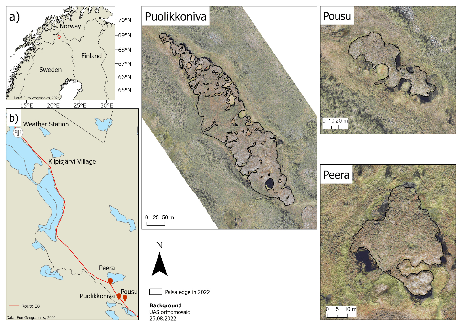
Figure 1 Location of the study sites Puolikkoniva, Pousu and Peera in northwestern Finland (a). Climate data used in this study are from the Kilpisjärvi weather station, from which the distance to the palsa sites is around 20 km (b). Base maps were obtained from EuroGeographics (2024).

2.1 Palsa mire sites

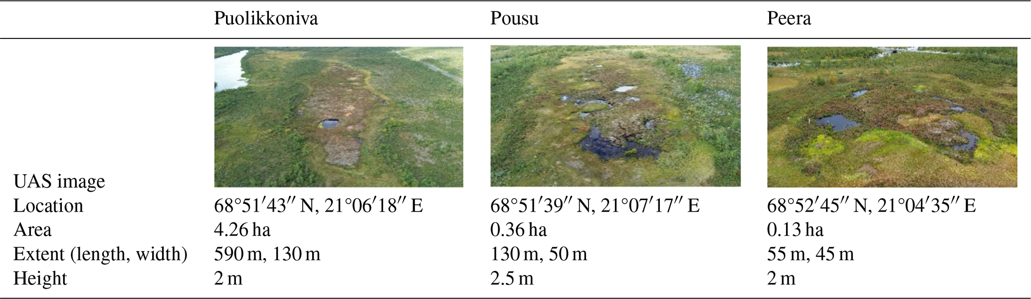
Puolikkoniva is located ca. 2.3 km south of Lake Peerajärvi at $\mathrm{68}\mathit{°}{\mathrm{51}}^{\prime }{\mathrm{43}}^{\prime \prime }$ N, $\mathrm{21}\mathit{°}{\mathrm{06}}^{\prime }{\mathrm{18}}^{\prime \prime }$ E and at around 455 m a.s.l. (metres above sea level), surrounded on the eastern side by the Könkämäeno River and extending to the west near the main road. The study site has an area of roughly 4.26 ha, with a maximum height difference relative to the surrounding peatland of ca. 2 m. This palsa is about 590 m in length and 130 m in width. Puolikkoniva is a prototypical longitudinal plateau palsa, consisting of several single shapes and some complex shapes. According to the definition from Seppälä (2006) and Meier (2015), the palsas contain a perennially frozen core of peat with segregated ice. Numerous cracks traverse the palsa site, with dwarf shrubs (5–20 cm high, e.g. Rubus chamaemorus, Empetrum hermaphroditum) and dwarf birches (5–60 cm high, Betula nana) at the edges, while atop and around the palsas, typical vegetation such as lichens (up to 3 cm high, e.g. Cetraria spp., Cladonia spp.) and sphagnum mosses (under 3 cm high, e.g. Sphagnum lindbergii) dominates. The absence of distinct dome-shaped structures and the presence of thermokarst ponds within the palsa structure indicate the degradation of the palsa (Seppälä, 2011), with pronounced block erosion at the steep edges (Table 1).

Pousu is located ca. 600 m east of the Puolikkoniva palsa at $\mathrm{68}\mathit{°}{\mathrm{51}}^{\prime }{\mathrm{39}}^{\prime \prime }$ N, $\mathrm{21}\mathit{°}{\mathrm{07}}^{\prime }{\mathrm{17}}^{\prime \prime }$ E and at around 470 m a.s.l., 150 m east of the main road. This study site covers an area of about 0.36 ha and has a maximum height difference relative to the surrounding peatland of ca. 2.5 m. This site, measuring 130 m in length and 50 m in width, is a classic example of a degrading dome-shaped palsa, as shown by collapsed parts, block erosion at its steep edges and thermokarst ponds within the former palsa structure. Similar to Puolikkoniva, typical palsa mire vegetation grows around and on it (Table 1).

Peera is located at $\mathrm{68}\mathit{°}{\mathrm{52}}^{\prime }{\mathrm{45}}^{\prime \prime }$ N, $\mathrm{21}\mathit{°}{\mathrm{04}}^{\prime }{\mathrm{35}}^{\prime \prime }$ E and at around 460 m a.s.l., ca. 400 m south of Lake Peerajärvi and 100 m west of the main road. This study site encompasses an area of about 0.13 ha and has a maximum height difference relative to the surrounding peatland of ca. 2 m. This palsa is about 55 m in length and 45 m in width. The palsa structure is surrounded by typical peatland vegetation such as sphagnum mosses and sedges. Water bodies, peat and bare-rock structures can be found at the edges of the palsa. Mainly lichens and dwarf shrubs grow on top of the palsa. Similar to Pousu, this palsa is also dome-shaped and in a degrading phase. Verdonen et al. (2023) point out a significant decrease in the surface area of the palsa during the past 15 to 60 years (Table 1).

Table 1 Main characteristics of each palsa site. Images were recorded with a DJI mini 3 Pro UAS on 30 August 2023.

2.2 Climate

The investigation areas are located in the pre-alpine belt of the Scandes. For the time period of 1991–2020, the annual mean temperature is −1.30 °C, the annual mean precipitation amount is about 515 mm and the dominant wind direction is south-southeast from November to April (FMI, 2022). Higher mountains influence local weather conditions; e.g. clouds are held up in front of mountains, or wind directions are influenced (Autio and Heikkinen, 2002). This may lead to different precipitation amounts or different wind directions and speeds than those measured at the Kilpisjärvi weather station (Verdonen et al., 2023). Also, high wind speeds during winter can lead to more intensive snow drift, influencing the snow distribution inside the mire sites (DeWalle and Rango, 2008).

The palsa mire sites are affected by cold winters and moderately warm summers (Fig. 2). Winter is the longest season, lasting about 200 d including the polar night, with around 50 d without sunlight. During winter, the temperature can drop close to −50 °C and can increase above 0 °C (FMI, 2024). In Kilpisjärvi, the duration of permanent snow cover lasts about 217 d yr⁻¹ (Lépy and Pasanen, 2017). During spring, the snow cover melts away, and the growing season starts in late May. In late August, the growing season ends with the beginning of autumn, which lasts around 102 d (Kauhanen, 2013).

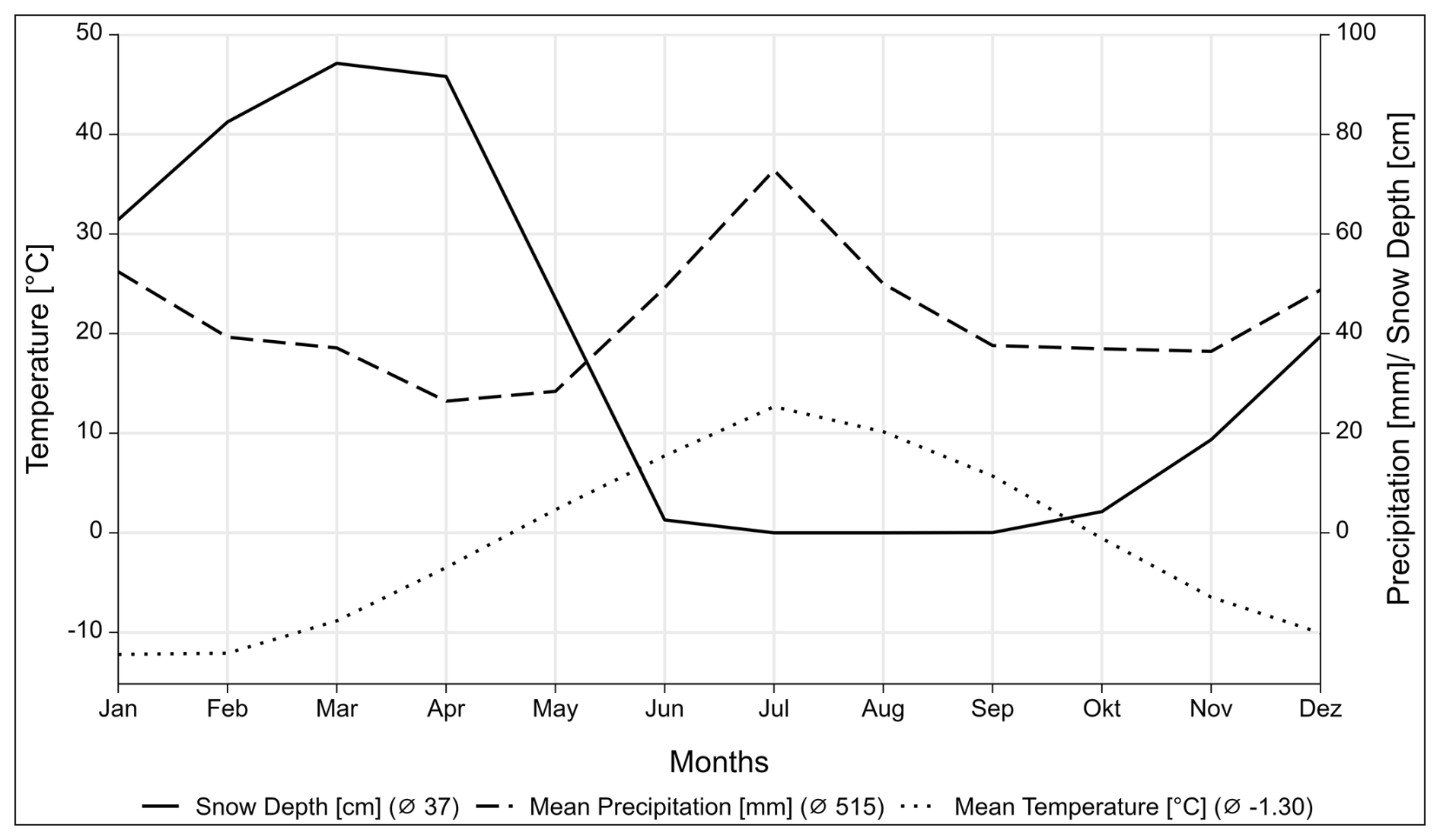
Figure 2 Climate chart of Kilpisjärvi (FMI, 2022). Climate data were measured at 69.03905 N, 20.81379 E and 474 m a.s.l. (metres above sea level) during the period of 1991–2020. The dotted line shows the temperature 2 m above ground in °C, the dashed line shows precipitation in mm and the solid line shows snow depth in centimetres. The Köppen–Geiger climate classification is Dfc.

3 Data and methods

In late August 2022 and late March 2023, field expeditions to the palsa mire sites were conducted to collect a comprehensive dataset consisting of UAS lidar data and in situ snow depth measurements for modelling purposes. Late August was chosen specifically for the collection of summer data, as it corresponds with the peak of the growing season and the maximum ALT, which typically occurs in this region by the end of August and mid-September, depending on the annual weather patterns and the onset of frost (Verdonen et al., 2023). This timing ensures the capture of the landscape's conditions in various states before the start of winter, providing the basis for extracting relevant input parameters for our approach. The input parameters are spatial datasets calculated on the basis of elevation data derived from UAS lidar.

On the contrary, late March was chosen for the winter dataset based on historical climatological patterns in the Kilpisjärvi region, which typically have maximum snow depths at this time (FMI, 2024). This period allowed for the collection of data under conditions that reflect winter extremes, which serves as both validation and training data for the RF modelling. Figure 3 shows an overview of the different steps carried out for this work.

Figure 3 General overview of the data collection and analysis.

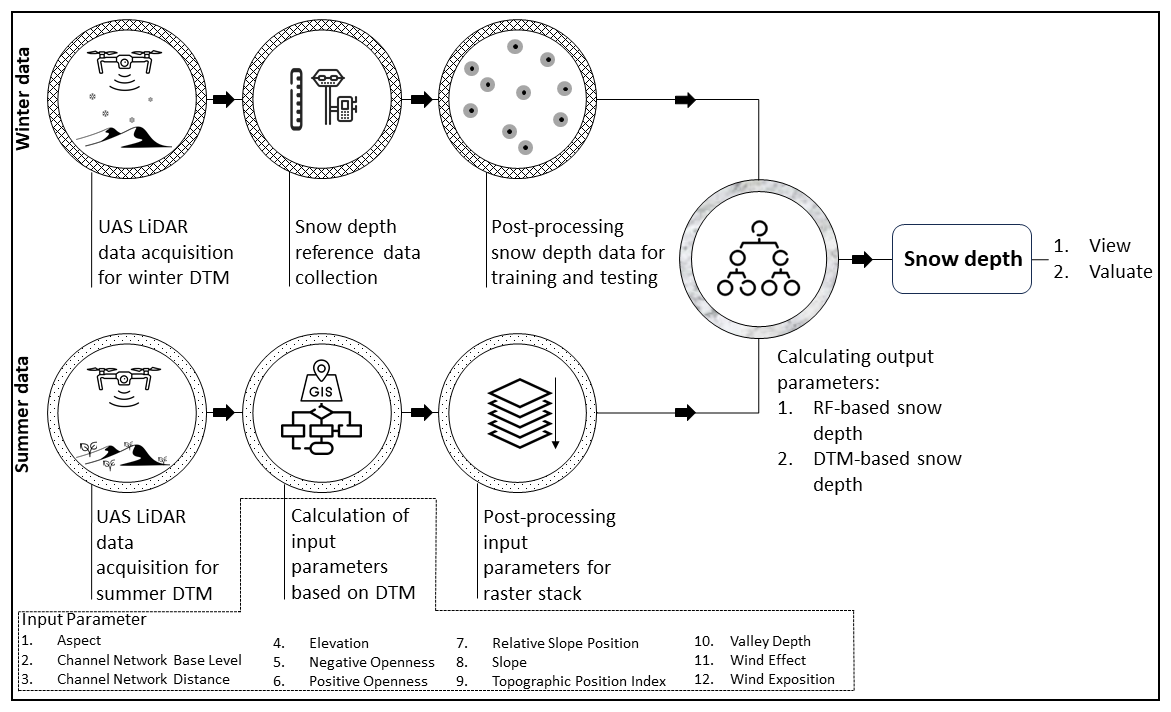
3.1 UAS data

3.1.1 UAS data collection

For the initial collection of UAS lidar data to generate the input parameters, aerial surveys were conducted at all three study sites on 27 August 2022 using a DJI Matrice 300 RTK equipped with a YellowScan Mapper+ lidar system that scanned at a wavelength of 905 nm. The flight altitude was 30 m for each palsa, with a 50 % side overlap. The flight direction was along the longitudinal axis of the palsas, except for Peera palsa, which followed an east–west orientation. The flight trajectories are pictured in Fig. 4. To improve the accuracy of the data collected, we used ground control points (GCPs) measured with a Trimble R12i real-time kinematic (RTK) global navigation satellite system (GNSS). We have established several permanent GCPs located on known points of large stones at the study sites. Permanent GCPs have been established because we are monitoring changes in the palsas by collecting drone data annually over the past 8 years. The accuracy of these RTK-GPS-measured GCPs is between 1 and 2 cm. For all UAS lidar summer flights, we utilized the following GCPs: 3 for Peera, 20 for Pousu and 30 for Puolikkoniva.

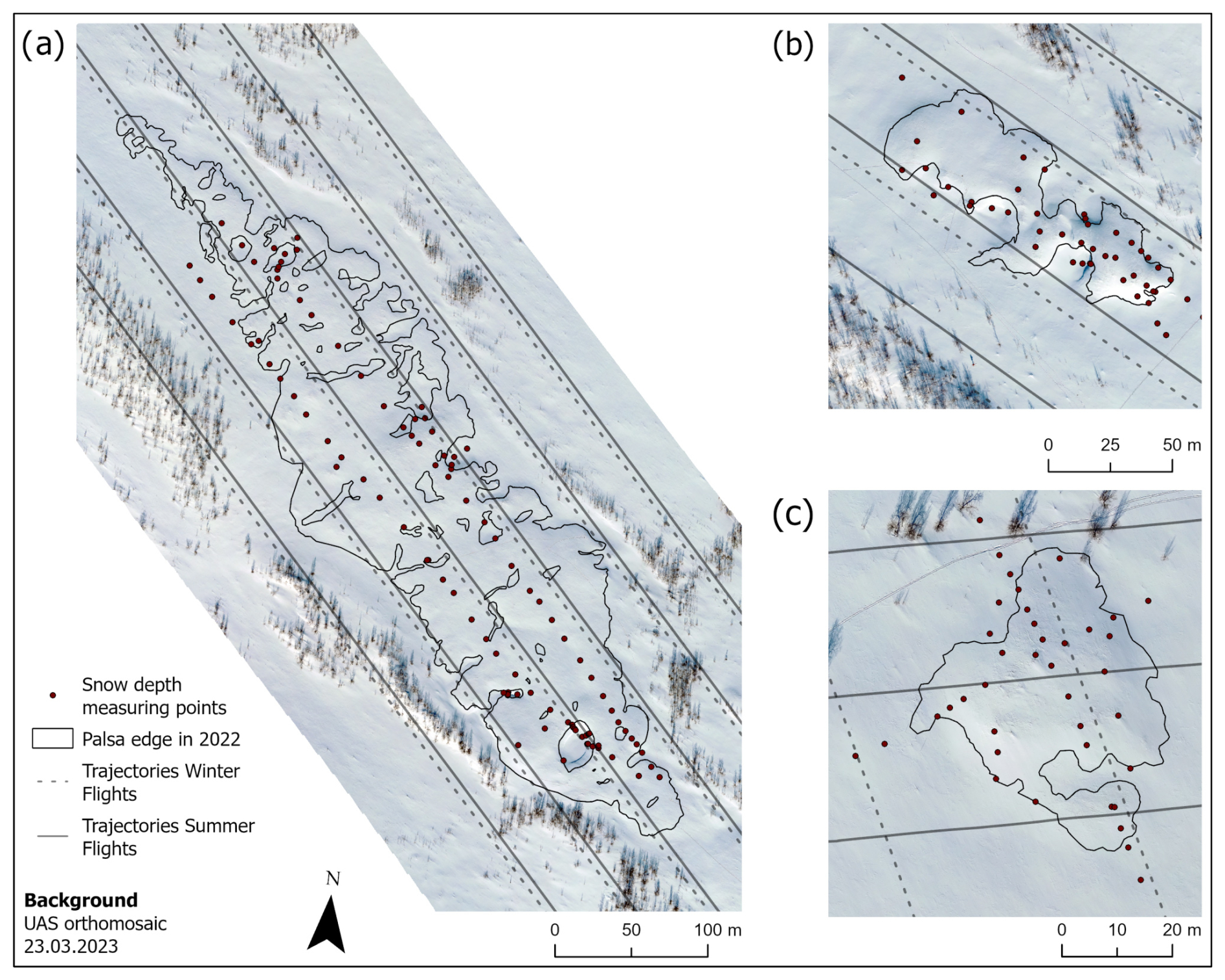
Figure 4 Snow depth measuring points within the investigation sites at Puolikkoniva (a), Pousu (b) and Peera (c) palsa, illustrating different methods for recording snow depth (transects, randomized and crossed).

The winter survey replicated the methodological framework of the summer survey using the same drone and sensor. The flights for all three study sites were carried out on 23 (Puolikkoniva and Pousu) and 24 March (Peera) 2023. The flight altitude was 60 m, with a 50 % side overlap. The flight direction was along the longitudinal axis of each palsa (see Fig. 4). For each site we used four GCPs, positioned around the palsa. The accuracy for each GCP is between 1 and 2 cm.

In addition, high-resolution RGB images were captured with an Autel EVO II Pro V2 to create an orthopicture of each palsa site during both surveys in Agisoft Metashape Professional software, enabling a comprehensive analysis of the site's conditions. The flight altitude was 80 m, with a 75 % side overlap for each flight. The RGB flights were conducted using the drone's internal RTK system.

3.1.2 UAS data post-processing

The lidar data acquired were post-processed using YellowScan CloudStation, resulting in point clouds for each flight. Mean point densities per square metre vary from 1064 (summer) to 831 (winter) for the Peera site, 308 to 338 for the Pousu site and 260 to 313 for the Puolikkoniva site. To refine the flight trajectories, we used receiver independent exchange format (RINEX) data in the position and orientation system post-processing software (POSPac). For each dataset, we obtained RINEX data from the continuously operating reference station (CORS) of the National Land Survey of Finland (NLS) in Kilpisjärvi (KILP, 2147250.4266, 820562.0462, 5930136.8831).

For noise and vegetation removal in the dataset, we used the progressive morphological filter (PMF) described by Zhang et al. (2003) and Jacobs et al. (2021) in order to create digital terrain models (DTMs). We applied filtering using window sizes of 0.5, 1, 2 and 3 and thresholds of 0.05, 0.1, 0.3 and 0.5. The ground points extracted were saved in point cloud format. Using the software CloudCompare, we generated a DTM for each flight mission in a 0.1 m×0.1 m resolution with the rasterize function. Empty cells within the point clouds were interpolated with a triangle max edge length value of 5.0.

Based on the summer and winter DTMs of the palsa sites, snow distribution datasets were calculated by subtracting the winter DTM from the summer DTM in the geographic information system (GIS) using ArcGIS Pro by Esri, allowing the comparison of UAS-lidar-measured (SD_lidar) and RF-modelled (SD_RF) snow depth.

3.2 Reference data collection

Additional datasets that are essential for modelling and validation were collected after the respective flights. Snow depth measurements (SD_{in situ}) were carried out manually using a wooden yardstick across all sites, where each point was measured at the snow cover surface by RTK GPS to find the exact location. On 23 March 2023, SD_{in situ} was measured at Puolikkoniva and Pousu and on 24 March 2023 at Peera. A total of 185 validation points were recorded, divided across the sites as follows: 100 in Puolikkoniva, 46 in Pousu and 39 in Peera (Fig. 4).

To ensure the derivation of a diverse SD_{in situ} training dataset, different measurement network designs were attempted at each site, customized to the unique geomorphological features of the palsa mires, making sure to catch points on top of the palsa, at the edges and at the steep slopes, on the thermokarst ponds, and in the surrounding field, as at those parts, differences in snow depth can be expected. At Pousu, a randomized sampling strategy was applied with a focus on the palsa edges and summits (Fig. 4b). At Puolikkoniva, there were two parallel transects measured following its longitude shape and complemented by randomized points at the edge, at the thermokarst and in the surrounding field (Fig. 4a). The Peera approach consisted of two intersecting transects, augmented by a set of randomly chosen points along the edge (Fig. 4c). This training dataset captures the variability in snow cover within palsa mires, ranging from snow-free palsa summits to deeply covered palsa edges, allowing the distribution of all SD_{in situ} into the point classes of edge, on top, open area and thermokarst. A histogram of SD_{in situ} data can be viewed in Appendix A1 and the distribution into the respective classes in Appendix A2.

3.3 Modelling data preparation

The lidar data collected from the summer flight missions were used to create the input parameters for the RF modelling in SAGA GIS by SourceForge. For that, we used the DTMs as input for the creation of all parameters and afterwards resampled these rasters to the same extent and resolution in ArcGIS Pro, making them suitable for analysis with the RF algorithm.

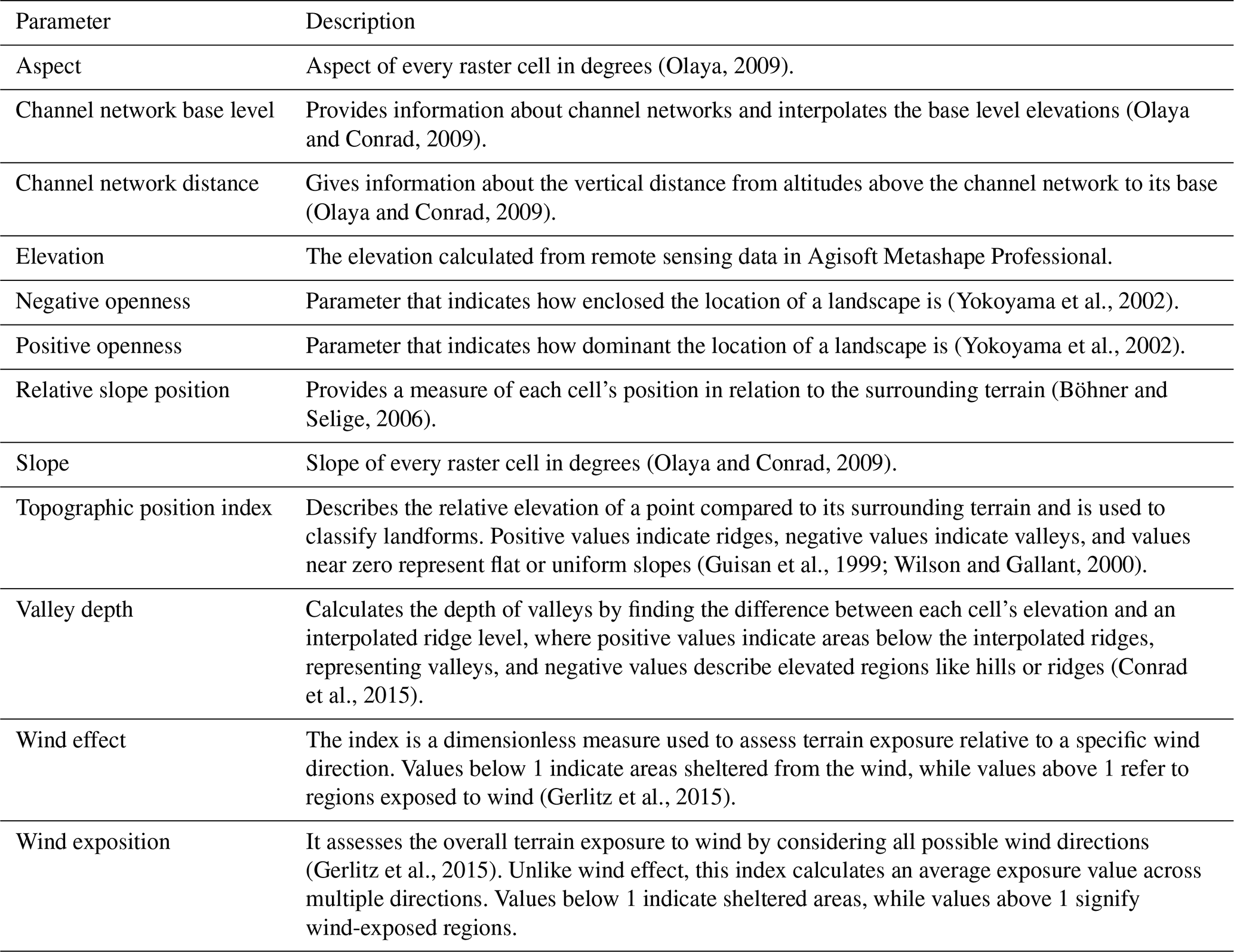
Subsequently, SAGA GIS was used for the computation of various geomorphological parameters to enhance the training dataset with a diverse range of topographical and environmental predictors. These predictors included elevation, aspect, slope, and a range of indices comprising hydrological and morphological landscape features (Table 2). According to Meloche et al. (2022) and Revuelto et al. (2020), the topographic position index (TPI) is of great relevance when modelling snow distributions due to its proven importance in representing dependencies between topography and snow depth.

(Olaya, 2009)(Olaya and Conrad, 2009)(Olaya and Conrad, 2009)(Yokoyama et al., 2002)(Yokoyama et al., 2002)(Böhner and Selige, 2006)(Olaya and Conrad, 2009)(Guisan et al., 1999; Wilson and Gallant, 2000)(Conrad et al., 2015)(Gerlitz et al., 2015)(Gerlitz et al., 2015)

Table 2 Overview of all input parameters used in the RF modelling.

3.4 Random forest algorithm

For the modelling process, we used the ranger package (Wright and Zigler, 2017) within the R programming environment, which is known for its ability to efficiently process large datasets and which accounts for complicated predictor interactions. The preparatory steps included aggregating the various input parameters into a uniform raster stack, conducted by the stack function from the raster package (Hijmans et al., 2023), ensuring spatial alignment across all layers.

The dependent variable for our model was the previous described SD_{in situ}. These measurements, together with the stacked input parameters (Table 2) as independent variables, formed the basis of our RF model. The SD_{in situ} locations, serving as the training dataset, were buffered by 0.3 m, with each buffered point assigned to the corresponding snow depth value. The process of extracting input parameter values from the stacked raster set was performed by randomly separating 70 % of the point features from each SD_{in situ} dataset for training and 30 % for testing. After this separation, we extracted the input parameter values for the training dataset, ensuring a clear distinction between training and testing data. The input parameters were not averaged within the buffer areas; instead, each parameter value was directly linked to the respective SD_{in situ} measurement. Consequently, each snow depth value is associated with an average of 28 input parameter values, leading to a dataset consisting of 3645 training values (Puolikkoniva = 1983, Pousu = 905 and Peera = 757) and 1577 test values (836, 401 and 340). The buffering strategy aimed to moderate model variability, reduce noise, minimize the influence of geolocation and sampling errors, and enhance the robustness of the model by increasing the number of training points. By incorporating groupings of nearby points rather than relying on single-point measurements, this approach helps improve the model's stability and realism, as demonstrated in Bergamo et al. (2023). To prevent errors and miscalculations, all no-data values were removed from the datasets, resulting in a final training dataset of 3504 points and a final test dataset of 1548 points for further modelling and validation.

To determine the optimal values for mtry, min.node.size and sample fraction, we performed hyperparameter tuning using the mlr package in R (Bischl et al., 2016). To prevent overfitting, we restricted the search range for min.node.size to 10–15 and for the sample fraction to 0.7–0.85, following the recommendations of Probst et al. (2019) and Breiman (2001). Allowing an unlimited search range initially resulted in better model performance but at the cost of reduced generalization, indicating signs of overfitting. We selected the final search range based on multiple test runs with different settings. For cross-validation, we tested different fold sizes to identify the most effective configuration. The best results were achieved using a four-fold cross-validation. The final tuned hyperparameters values were as follows: mtry = 9, min.node.size = 10 and sample fraction = 0.79.

Permutation mode was chosen for variable importance assessment, and a specific seed value was implemented to ensure the reproducibility of the results. For more robustness, we repeated the calculation 100 times to obtain a mean permutation importance (PI) value for each input parameter, ensuring reliable rankings. The resulting PI values for each input parameter were normalized for better comparison by setting the most important parameter to 1. Subsequently, the trained RF model was employed to calculate SD_RF predictions across each palsa site using the predict function.

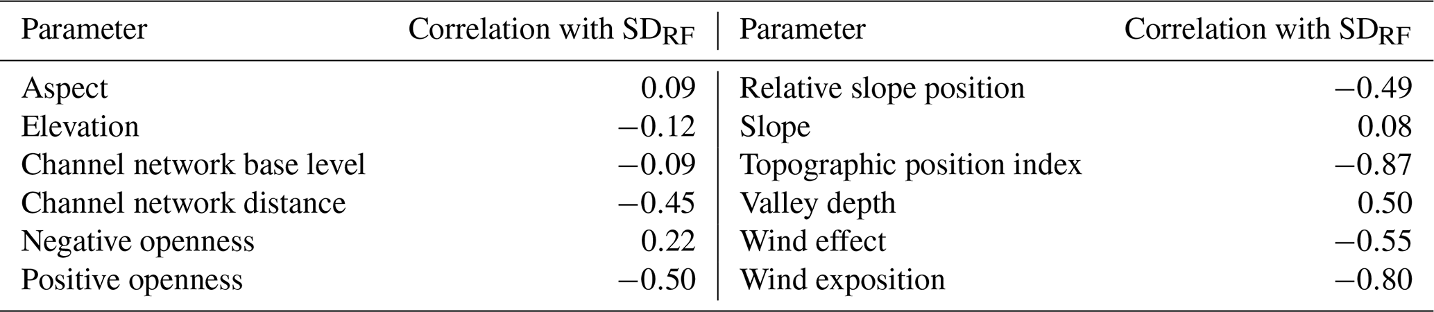
Additionally, a correlation analysis between the input parameters and predicted SD_RF was performed to identify any correlating predictors and assess the strength of the relationships between them and the prediction. Correlation values for all input parameters are listed in Appendix A3. Furthermore, the RF model was run three additional times to ensure a fully external validation. In each run, one palsa site was excluded from the training data, allowing its measured SD_{in situ} values to be used exclusively for validation.

3.5 Statistical analysis

The statistical analysis focused on evaluating the predictive accuracy of the model. The following metrics were summarized for all palsa sites and calculated in the R environment.

1. Coefficient of determination (R²). Calculated to quantify the proportion of variance in the dependent variable that is predictable from the independent variables in the model (Nagelkerke, 1991), it gives clarity about the overall effectiveness of the model, defined as

   $$\begin{array}{}\text{(1)}& R^{\mathrm{2}}=\mathrm{1}-{\displaystyle \frac{\sum (y_i-{\widehat{y}}_i{)}^{\mathrm{2}}}{\sum (y_i-\stackrel{\mathrm{‾}}{y}{)}^{\mathrm{2}}}}.\end{array}$$

2. Root-mean-square error (RMSE). Employed to quantify the average magnitude of the error in the predictions (Chai and Draxler, 2014), it highlights the ability of the model to predict snow depth accurately, defined as

   $$\begin{array}{}\text{(2)}& \text{RMSE}=\sqrt{{\displaystyle \frac{\mathrm{1}}{n}}\sum (y_i-{\widehat{y}}_i{)}^{\mathrm{2}}}.\end{array}$$

3. Mean absolute error (MAE). This measures the average magnitude of the absolute errors between predicted and observed values without considering their direction (Chai and Draxler, 2014; Willmott and Matsuura, 2005), defined as

   $$\begin{array}{}\text{(3)}& \text{MAE}={\displaystyle \frac{\mathrm{1}}{n}}\sum _{i=\mathrm{1}}^n|y_i-{\widehat{y}}_i|.\end{array}$$

4. Standard deviation (SD). This provides a measure of the dispersion of prediction errors around their mean (Walser, 2011), revealing the precision and consistency of the predictions, defined as

   $$\begin{array}{}\text{(4)}& \text{SD}=\sqrt{{\displaystyle \frac{\mathrm{1}}{n-\mathrm{1}}}\sum _{i=\mathrm{1}}^n(y_i-{\widehat{y}}_i{)}^{\mathrm{2}}},\end{array}$$

where y_i is the observed value, ${\widehat{y}}_i$ is the predicted value from the model and $\stackrel{\mathrm{‾}}{y}$ is the mean of the observed values.

To visualize the statistical analysis results, scatter plots were created to compare RF- and UAS-lidar-derived snow depths with the test dataset values.

4 Results

4.1 Snow depth predictions

In general, the predicted SD_RF presents good visual alignment with the calculated SD_lidar (Fig. 5).

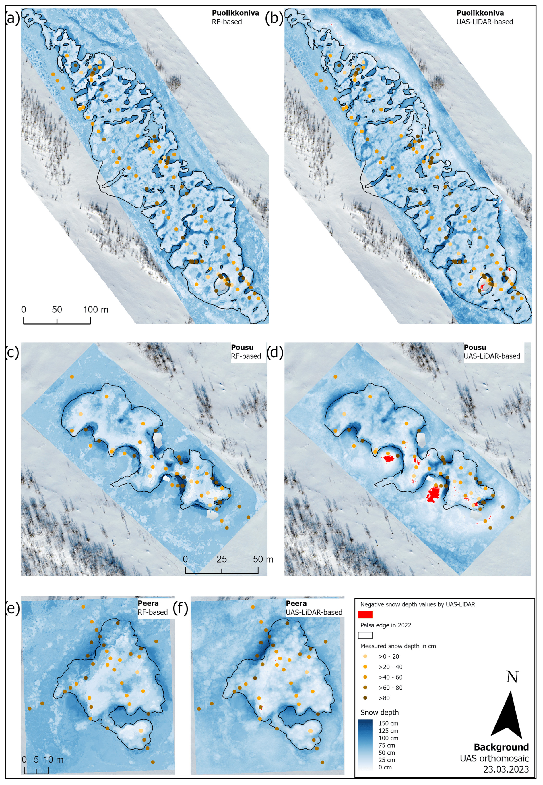
Figure 5 Snow depth predictions based on the RF model (a, c, e) and the UAS lidar (b, d, f) at the Puolikkoniva (a, b), Pousu (c, d) and Peera (e, f) palsa sites. Yellow/brown points indicate SD_{in situ} locations and represent measured snow depth. In the lidar results, red-coloured areas correspond to negative snow depth values, which result from elevation mismatches between the summer and winter DTMs.

The Puolikkoniva palsa site is affected by several collapsed areas in which snow accumulates heavily. This can be seen in the SD_RF (Fig. 5a) as well as in the SD_lidar (Fig. 5b) results. On the eastern side of the palsa, RF models the snow depth inside these collapsed holes and cracks higher than the UAS lidar detected it. Directly at the steep edges of the palsa in particular, the depth values increase up to 20–40 cm and in places up to 60 cm. On the western side of the palsa, SD_lidar is higher, with values increasing up to 20–40 cm compared to SD_RF. However, the transition of the snow depths corresponds to changes at slopes in the UAS lidar results better, as the RF model reveals obvious patterns. The most obvious differences occur in areas beneath the palsa itself, for example the entirety of the northeastern and eastern parts that are directly at the edge of the palsa, which have higher snow depths (up to 60 cm) predicted by RF than were detected based on the UAS lidar data. Within the open area beneath the palsa, SD_lidar is higher (up to 50 cm), following areas with higher vegetation. The most similar parts are the areas on top of the palsa, with differences between both datasets under 15 cm and in places 20 cm. The UAS lidar dataset includes negative snow depth values, which result from elevation mismatches between the summer and winter DTMs. These are visualized in red to distinguish them clearly in Fig. 5.

The Pousu palsa site shows a similar pattern to the Puolikkoniva palsa site, with cracks filled by snow and collapsed parts with steep slopes where snow has accumulated heavily (Fig. 5c and d). Again, the transition of the snow depth at those areas is more natural in the SD_lidar data since the SD_RF data show sharp steps. Also, mire areas next to the palsa were observed by UAS lidar to have lower snow depth than those modelled with RF. This is especially visible in the southwestern and southern parts of the area, where snow depth was modelled between 40 and 50 cm, and the UAS lidar detected values between 10 and 20 cm. However, similarities are visible on top of the palsa, where snow depths were modelled and observed in a range between 10 and 30 cm each.

The Peera palsa site shows the highest consistency between SD_RF and SD_lidar. However, similarly to the other two sites, the highest snow depth accumulated in cracks and at the steep edges of the palsa (Fig. 5e and f). Unlike at the other locations, there are no sharp steps at the parts mentioned here, as both approaches model smooth transitions. Similar structures are also visible on top of the palsa, with snow depths around 20 cm in each approach. However, differences similar to those at the two other palsa sites are visible in the area surrounding the palsa, where the RF calculated the snow depth higher than the UAS lidar detected it. Higher snow depths were also calculated by RF on the northwestern edge of the palsa than were measured with lidar (up to 30–50 cm).

Viewing the deviations in snow depth between the two approaches, it is evident that the top parts of the palsa sites themselves show very small differences (Fig. 6a–c). However, deviations occurred at the edges, inside of cracks, at the highest parts of the palsa and in the surrounding areas. Within cracks on top of the palsa sites, in general, the UAS lidar detected higher snow depth than the RF modelled, except for the eastern side of Puolikkoniva palsa, where it is the other way around. Differences of around 20 cm are shown but with peaks up to 60 cm. Also, the highest-elevation structures of the palsa sites directly at the edges show deviations of about 15–40 cm higher snow depth calculated by the UAS lidar, except for at Peera palsa. In contrast, the collapsed parts with accumulated snow are consistently modelled with higher values, exceeding a deviation of 45 cm compared to the UAS-lidar-derived values. Notably, deviations in the areas surrounding the palsas are primarily characterized by the higher snow depths predicted by the RF model, with the exception of areas with higher vegetation at the Puolikkoniva palsa site.

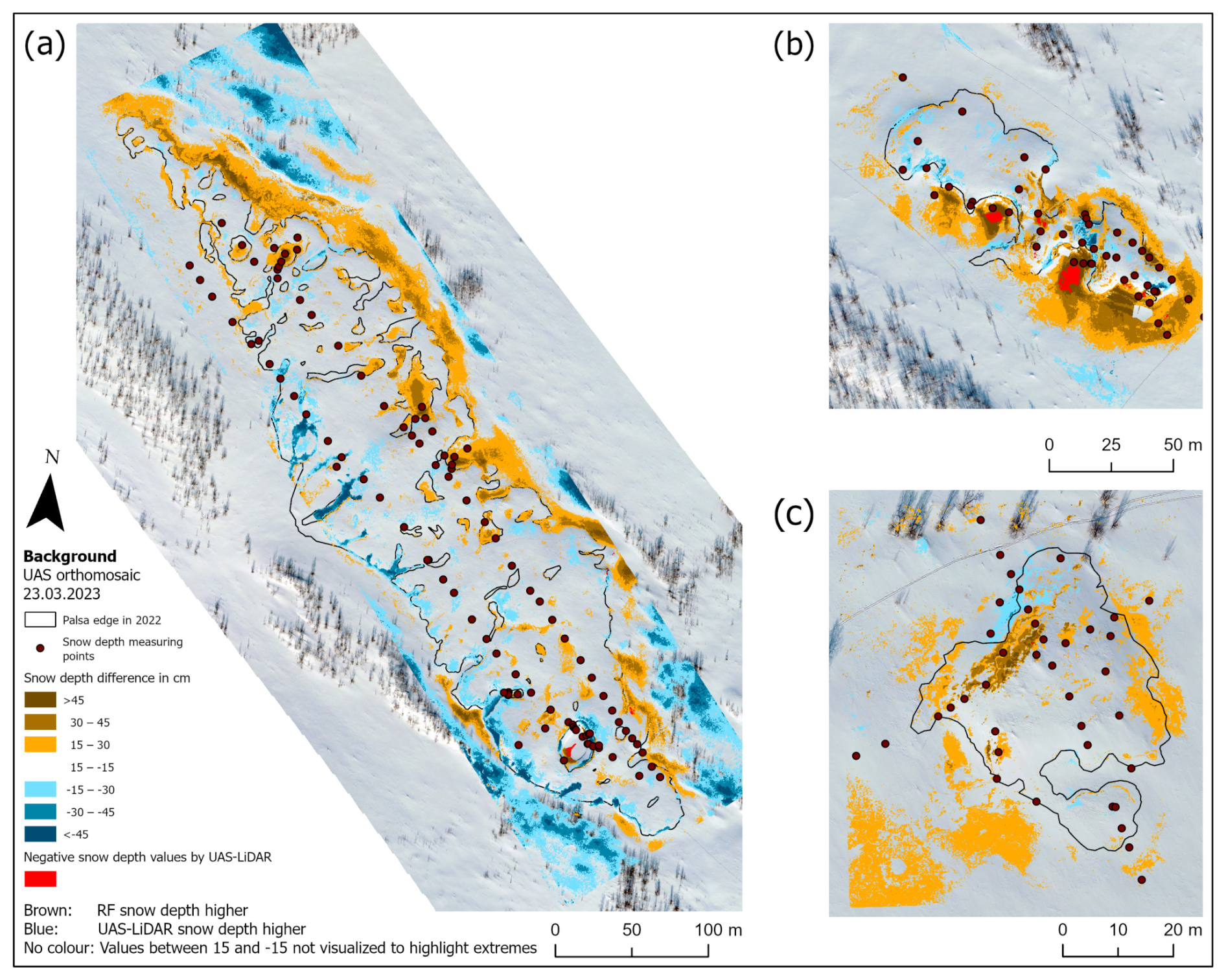
Figure 6 Snow depth differences between modelled and UAS lidar results at the (a) Puolikkoniva, (b) Pousu and (c) Peera palsas.

4.2 Variable importance

The calculated PI values of all parameters are pictured in Fig. 7. The four most important parameters are TPI, wind exposition, elevation and channel network base level; TPI is the most important parameter and is set to 1. It is more than four times more significant than the next two parameters, wind exposition (around 0.14) and elevation (0.13). In addition, channel network base level (0.12), wind effect (0.08) and valley depth (0.07) are also of substantial importance. The remaining input parameters, positive openness, channel network distance, relative slope position, negative openness, slope and aspect, possess importance lower than 0.04.

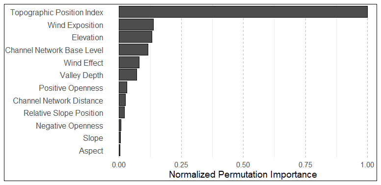
Figure 7 Overview of the normalized mean permutation importance values from RF modelling over 100 iterations.

4.3 Statistical evaluation results

The statistical analysis of the general accuracy (Table 3) and validation point location accuracy (Table 4) reveals comparable high accuracy of SD_RF and SD_lidar. The RF modelling dataset has slightly better statistical validation metrics than the SD_lidar dataset, with a RMSE of 18.33 cm compared to 23.49 cm. Furthermore, R², MAE and SD are better in the RF modelling, with values of 0.770, 13.26 and 18.11 cm compared to 0.691, 17.49 and 20.84 cm. The external validation results of the RF modelling dataset for each palsa (Table 3) indicate the best performance at the Peera site, with an RMSE of 16.67 cm and an R² of 0.628. At the Pousu site, the RMSE is higher (21.31 cm), but the R² improves to 0.767. The Puolikkoniva site shows the weakest performance, with both metrics being the lowest: an RMSE of 27.13 cm and an R² of 0.578.

Table 3 Overview of the calculated root-mean-square error (RMSE) in centimetres, the coefficient of determination (R²), mean absolute error (MAE) in centimetres and standard deviation (SD) in centimetres for RF- and UAS-lidar-derived snow depth estimations. Additionally, external validation results for RF-modelled snow depth at each palsa site (Peera RF, Pousu RF and Puolikkoniva RF) are provided.

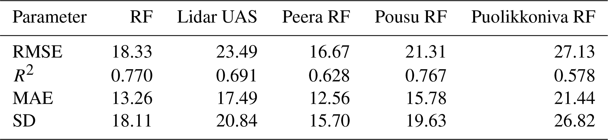
Table 4 Overview of RMSE (cm), R², MAE (cm) and SD (cm) divided into the validation point locations within the investigation areas.

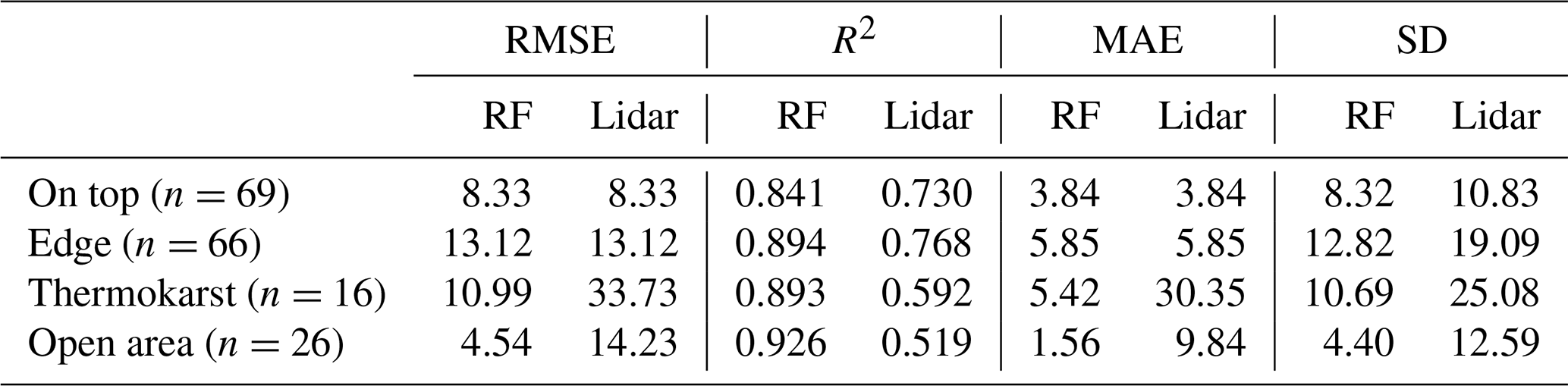
When analysed by point groups, the SD_RF and SD_lidar results show strong similarities for the on-top and edge classes, while the thermokarst and open-area classes exhibit better metrics in the SD_RF dataset. RMSE and MAE values are identical for both datasets in the on-top (8.33 cm, 3.84 cm) and edge (13.12 cm, 5.85 cm) groups, but R² is higher for SD_RF (on top = 0.841, edge = 0.894) compared to SD_lidar (0.730, 0.768). A similar trend is observed for the standard deviation, with values of 8.32 cm vs. 10.83 cm in the on-top class and 12.82 cm vs. 19.09 cm in the edge class. The thermokarst class consistently shows better metrics in SD_RF compared to in SD_lidar, with RMSE of 10.99 cm compared to 33.73 cm, R² of 0.893 to 0.592, MAE of 5.42 to 30.35 cm and SD of 10.69 to 25.08 cm. A similar pattern is observed for the open-area class, where RMSE improves from 14.23 cm (SD_lidar) to 4.45 cm (SD_RF), R² from 0.519 to 0.926, MAE from 9.84 to 1.56 cm and SD from 12.59 to 4.40 cm.

The scatter plots of both approaches (Fig. 8) reveal further insights into the accuracy of the results. Both SD_lidar (left plot) and SD_RF (right plot) show a positive correlation with SD_{in situ}. The regression line in both plots closely follows the expected trend, showing that both methods capture snow depth patterns well. The SD_RF results exhibit a tighter spread around the regression line, indicating lower variance compared to SD_lidar. This is consistent with the standard deviation values reported in Table 4, where SD_RF shows a 13 %–65 % lower spread across validation point groups. The spread of residuals (black dots deviating from the regression line) increases with snow depth in both cases, indicating larger uncertainty for deeper snow, while the confidence intervals remain narrow at lower snow depths. A single negative outlier is present for SD_lidar.

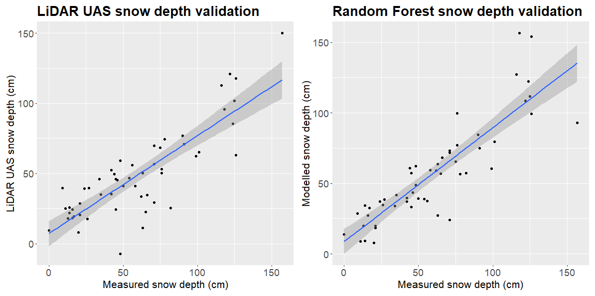
Figure 8 Scatter plots with regression lines for UAS-lidar-derived and RF-modelled snow depths based on the external test dataset.

In addition, the correlation analysis between the input parameters and SD_RF reveals a strong negative correlation with TPI (−0.87) and wind exposition (−0.80). Moderately high negative correlations are observed for wind effect (−0.50), positive openness (−0.50), relative slope position (−0.49) and channel network distance (−0.45). The only moderately high positive correlation is given for valley depth, 0.50. All other parameters show low correlations, with values close to zero.

5 Discussion

5.1 Analysis of RF and lidar snow mapping

The statistical analysis of SD_RF and SD_lidar demonstrates statistically significant and reliable results for both approaches. The overall metrics of RMSE and R² for RF and lidar indicate slightly better performance of the RF model in mapping snow distribution (Table 3). This trend is also evident in the visual comparison, although a more detailed examination reveals important differences between the two methods. The external validation across all palsa sites confirms the sufficient accuracy of the RF model (Table 3), while the scatter plots (Fig. 8) show strong consistency between the two approaches.

In both approaches, the upper parts of the palsa, which are relatively flat and covered with low vegetation, have similar snow depth values. This is also confirmed by the identical RMSEs for the point group on top (Table 4). Since these areas are well represented in the training dataset for the RF approach, and the surface captured by UAS lidar changes only slightly between summer and winter in the stable area of the palsa, both methods estimate snow depth well. The accuracy of the RF models depends to a large extent on the quality of the training data, which is the reason a well-distributed dataset is essential. However, as the surface variations on the top of the palsas are minimal, the acquisition of representative training data is relatively easy, which explains the high accuracy of the model in these areas. The same considerations apply to the UAS lidar data. Due to the low vegetation cover, only minimal vegetation removal was required during post-processing, reducing potential sources of error in these areas. However, the seasonal changes in ground level in palsa mires must also be taken into account. Frost heave and subsidence cause natural height variations of several centimetres between summer and winter, as recently described by Renette et al. (2024). If the UAS lidar dataset is acquired in spring immediately after snowmelt, when the ALT has reached its minimum thawing depth, such effects could be minimized. In addition, RTK GPS point data from field measurements in winter and summer could help to correct elevation differences by calculating mean elevation shifts. However, this method has its own challenges, as measuring ground level in winter is difficult due to the overlying snow cover. These seasonal variations in elevation should be carefully considered when deriving snow distribution from multi-season DTMs. In contrast, RF is expected to be less affected by this problem, as the modelled snow depth values are derived from training data and are not directly based on the absolute elevation differences between summer and winter datasets.

Similar patterns are observed for the steep edges of the palsa. While the RF model performs lowest for the edge point class within its own results, the lidar approach achieves its second-best performance in this category. Despite these internal differences, both methods produce identical RMSE values of 13.12 cm (Table 4). However, when interpreting lidar data, there are additional challenges at the palsa edges due to continuous degradation processes that lead to differences between the summer and winter DTMs. During summer data collection, the palsa edges are recorded before block erosion occurs, meaning that loose soil remains intact. By winter, block erosion and soil displacement may alter the terrain, leading to higher deviations between the DTMs. As a result, the SD_lidar values are artificially increased even though the actual snow depth is lower. A similar problem arises if cracks form after data collection in summer, which accumulate snow in winter and further increase the calculated snow depths. At the same time, these degradation processes are also not considered in the RF approach, as the summer dataset was used to derive all input parameters. This explains why RF struggles the most at the edges. In addition, the redistribution and accumulation of snow on steep slopes is a highly dynamic and chaotic process that is difficult to capture with high precision.

In contrast to other areas of the palsa, the RF and UAS lidar approaches show the lowest agreement over thermokarst pond areas, which is reflected in the statistical metrics for the thermokarst point class. Although these areas are covered in snow during winter lidar acquisition, they are characterized by open water surfaces in the summer dataset used to derive snow depth by DTM subtraction. This leads to an underestimation of terrain height in the summer DTM due to the low reflectivity and absorption of the lidar signal over water surfaces (Mandlburger and Jutzi, 2019), resulting in an overestimation of snow depth. In contrast, RF modelling benefits from the contextual relationships between the terrain parameters and the observed snow depth over thermokarst ponds and can partially compensate for such systematic errors, maintaining higher accuracy. Even though volumetric scattering in snow can affect lidar results, the associated error at the wavelengths commonly used for snow depth measurements, such as the 905 nm wavelength applied in this study, is typically in the low centimetre range (Deems et al., 2013) and thus does not account for the larger discrepancies observed in this study.

In addition, in mire areas surrounding the palsa, such as the statistics for the open-area point class, the RF model performs with the highest accuracy within its own results, while UAS lidar ranks second lowest. However, for UAS lidar, the deviation from the two best-performing groups, on top and edge, remains relatively small, indicating a consistent performance across the dataset. A significant challenge in these areas is the seasonal vegetation dynamics. In summer, the vegetation in palsa mires grows taller and denser, while in winter the grasses and sedges are compressed under the weight of the snow. The lidar sensor records all surface elements, i.e. the vegetation in summer and the snow-covered areas in winter. Despite the removal of vegetation in post-processing, a residual bias remains due to the dense vegetation, which cannot be completely filtered out from the ground, leading to a systematic underestimation of snow depth in areas with height-changing vegetation. Similar problems with lidar-derived snow depth mapping were reported by Broxton et al. (2019). Tall shrubs such as Betula nana, which form thickets at palsa edges, can further complicate the detailed capture of the palsa surface. In contrast, the RF model inherently accounts for vegetation, as it uses UAS lidar summer data as the basis for calculating input parameters. By integrating SD_{in situ} measurements from winter, RF can establish relationships between vegetation and snow accumulation, which reduces bias and improves snow depth estimation. Methods to further improve lidar-derived snow depth mapping, such as correcting estimates based on vegetation type, density and height, could help to mitigate these limitations.

These results confirm that snow distribution can be accurately modelled at the small scale using low-cost equipment, such as a yardstick, in combination with moderate computational resources. However, we acknowledge that an expensive lidar sensor was used in this study to derive the input parameters for the RF model. Therefore, further research should investigate whether low-cost UAS RGB data can provide equally high-quality input parameters or whether lidar is still essential for accurate modelling. Recent studies by Harder et al. (2020) and Cho et al. (2024) have shown that snow depths derived from UAS lidar data provide a more accurate representation of snow distribution than snow depth products derived from UAS RGB data, which raises the question of whether the use of RGB-derived input parameters is feasible for modelling purposes. However, for large-scale spatial snow distribution overviews or in cases where high-resolution snow depth mapping is not required, UAS lidar or RGB data might be preferable, as manual snow depth measurements are connected with a high workload and considerable time investment. Furthermore, the potential of UAS imagery for snow depth estimation has been investigated in several recent studies (Marti et al., 2016; Rauhala et al., 2023; Revuelto et al., 2021; Walker et al., 2021), emphasizing its growing importance for snow distribution monitoring.

5.2 Snow distribution mapping in palsa mires and its impacts

The high-resolution snow depth maps produced in this study provide a detailed spatial representation of snow distribution patterns in palsa mires and highlight pronounced warming and cooling areas. Both the lidar and RF datasets show similar small-scale variations that are closely linked to topographic features. These findings suggest that the observed snow distribution patterns accurately reflect the actual conditions in the palsa landscapes studied, making them valuable for assessing the potential interactions between snow accumulation and palsa thermal dynamics.

Warming areas in the palsas were identified at the edges of the palsa and in cracks where snow accumulates due to wind transport and gravitational sliding. This effect is consistent with the findings of Peng et al. (2024), who showed that snow accumulation insulates the ground and reduces the penetration of cold air. An example of this effect can be seen at Pousu palsa (Fig. 9d and e), where the dominant south and southwest winds (FMI data for the last 20 years from the Kilpisjärvi weather station) contribute to the highest snow accumulation at the southwestern and northeastern edges. Snow accumulation in these areas extends snowmelt into late spring and summer and increases soil moisture, which can increase heat transfer to the soil. While extended snow cover reduces direct solar radiation, it also prevents deep freezing in winter, which can destabilize ice core edges. This also leads to a thinner ALT at the edges, as the solar radiation remains limited due to the longer-lasting snow cover. These observations are consistent with the results of Verdonen et al. (2023) and Seppälä (2011). Such processes can contribute to block erosion and expose the frozen core to further thawing. The formation of cracks in the upper edge zones could also increase this effect, as they fill with snow in winter, delaying freezing and possibly further accelerating the instability of the palsa. These results are consistent with those of Martin et al. (2021), who showed that palsas undergo structural adjustments at constant snow depths of 20–30 cm. However, our results indicate that in the Kilpisjärvi region, even greater snow depths occur at the palsa edges, suggesting that the increasing snow accumulation may be linked to the continuing degradation of the palsas. This cycle continues until the palsa slopes flatten, reducing snow accumulation, which eventually leads to the degradation of the upper plateau. Long-term ALT and permafrost temperature measurements at these sites are needed to confirm this hypothesis. As proposed by Seppälä (2011), snow conditions may play a more important role in the development of palsas than previously thought. Continued monitoring and integration of these findings into permafrost models will be essential for a better understanding of future palsa development.

Figure 9 Demonstration of differences between UAS-lidar-derived and RF-modelled snow depths.

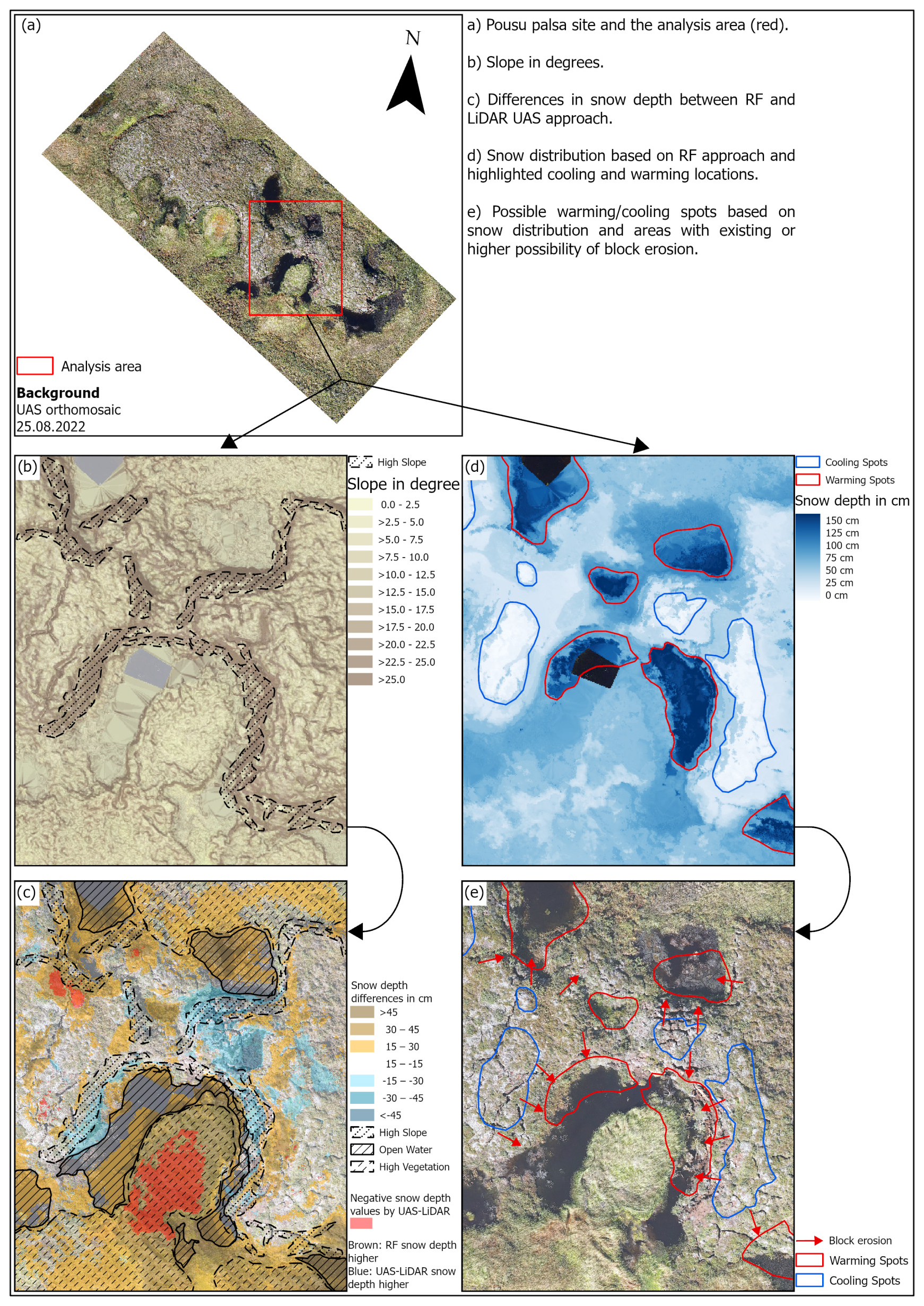
The uppermost parts of the palsa summits are cooling areas, where thin layers of snow allow cold air to penetrate deeper, which promotes ice core stability in winter. Seppälä (2003) proved that thicker snow cover on the palsas delays the melting of the ice core due to its prolonged presence. Conversely, this means that cooling areas have deeper ALTs in summer than warming areas do. As observed at Pousu palsa (Fig. 9b and c), the cooling areas are concentrated at the uppermost parts of the steep edges, where the surface is highly exposed to the wind. Further investigation is needed to determine whether this, combined with destabilization and edge collapse, contributes to the formation of steep or even vertical slopes. If this process continues, cracks may eventually form, causing block erosion and degradation of the palsa edge.

The findings of this study suggest that snow depth variability plays a crucial role in the stability of the palsa, with small-scale redistribution patterns influencing local permafrost dynamics. However, as this analysis is only based on snow depth data, further research combining continuous monitoring of snow depth with thermal observations of permafrost is needed to confirm these interactions. Establishing a direct link between snow accumulation patterns and thermal processes in the subsurface would provide valuable insights into the long-term evolution of palsa mires under changing climatic conditions. Furthermore, our study indicates that there is a clear need for more detailed research on the interaction between tall shrubs, snow depth and permafrost.

5.3 Uncertainties and limitations

Snow distribution is highly variable, especially because of wind drifts and topography, which must be considered when applying these methods. Additionally, machine learning models rely on unique observations in time. Changing weather conditions could result in a completely different snow distribution on another day, which could affect model performance.

Several sources of error can affect lidar-derived snow depth measurements during both summer and winter data acquisition. Reflective or complex surfaces, such as water or vegetation, may scatter or block the laser signal, introducing measurement biases and limiting surface detectability (Deems et al., 2013; Gould et al., 2013). These distortions impact the entire modelling approach, as they influence the calculation of the input parameters. Another source of uncertainty is the choice of lidar wavelength. The 905 nm wavelength used in this study is typical of many airborne systems and generally produces only minor depth errors in snow due to limited penetration, with most of the signal returned from the upper centimetres of the snowpack (Deems et al., 2013). In comparison, shortwave infrared wavelengths such as 1550 nm are more strongly absorbed by ice, resulting in a return signal that is more confined to the snow surface. This characteristic can help reduce uncertainty, particularly in areas with complex surface conditions or low reflectivity. While the wavelength-related interaction with the snow surface is a key factor, detailed information on snow conditions, such as grain size, snow age or impurity content, was not collected during the field campaign. Such data could, however, help to better assess potential sources of uncertainty in the lidar-derived snow depth, particularly those related to scattering and absorption effects. Errors can also occur when collecting training data, albeit to a less significant extent. Measuring with a yardstick is a reliable method of measuring snow depth, but dense layers of ice or vegetation close to the ground, such as roots, can change the recorded values by a few centimetres, as the ground surface would be incorrectly assumed. In areas with denser vegetation, the probe may not always reach the exact ground surface, resulting in a slight underestimation of the snow depth. This could affect both the training and validation of the RF model and the accuracy of the lidar-derived snow distributions, thus affecting the statistical performance of the results. Devices that have been developed only for taking snow depth values, such as the GPS Magnaprobe used in a study by Walker et al. (2021), could minimize the possibility of such errors.

The selection of input parameters is another aspect that requires critical evaluation. The TPI plays a central role in the model, as it combines several topographic features into a single parameter. As snow tends to accumulate at the edges and drift down the slopes, its movement from one grid cell to the next is effectively captured by the TPI, making it a crucial variable for the model. This finding is in line with studies by Revuelto et al. (2020) and Meloche et al. (2022), which highlight the importance of TPI for modelling snow distribution. Other important parameters are related to wind properties and basic surface structures, which emphasizes the importance of wind drift and steep edges in snow distribution formation. However, it should be noted that the parameters selected represent only a fraction of the potential variables that influence snow distribution. The RF model is theoretically capable of incorporating a larger set of parameters and still identifying the most significant ones. For example, detailed vegetation classifications – including specific vegetation types or density indices – could further improve snow depth modelling. In addition, there are influencing factors that, while not directly related to snow depth, can still have an impact on snow distribution patterns. The identification of such variables would require a specific study aimed at evaluating and selecting the most important parameters for snow depth modelling.

6 Conclusions

We present an analysis of snow distribution in palsa mires using a combination of in situ measurements, UAS lidar data and RF modelling. This study provides valuable insights into small-scale snow distribution, revealing distinct accumulation patterns at palsa edges and cracks driven by wind effects and gravitational sliding. The increased snow depth in these areas prolongs snowmelt, which could influence thermal insulation and ALT dynamics of permafrost. In contrast, the exposed palsa areas exhibit thinner snow cover, promoting deeper frost penetration in winter but also greater exposure to solar radiation in summer. Statistically, both RF modelling and UAS lidar provided reliable results for mapping snow distribution, with an RMSE of 18.33 cm (RF) and 23.49 cm (lidar) and corresponding R² values of 0.77 and 0.691. While the RF model showed slightly better prediction performance, the differences between the two approaches remained moderate. This indicates that RF modelling is a promising approach for snow depth estimation, especially when appropriate input parameters such as TPI and wind-related parameters are included. At the same time, UAS lidar provides a direct, high-resolution snow depth dataset and is therefore a valuable tool for spatial snow mapping.

Our results highlight the vulnerability of palsas to changes in snow depth patterns due to climate warming. A change in snow depth and altered wind dynamics could further accelerate the degradation of palsas and lead to a progressive loss of permafrost soils in northern Finnish Lapland. Future studies should focus on integrating long-term permafrost monitoring with these snow distribution models to better understand the interactions between snow cover, permafrost thaw and climate change. The methodology presented here provides a foundation for further modelling approaches that integrate snow distribution dynamics with permafrost development. While tested for palsa environments, the approach can also be applied to other pan-Arctic palsa areas and continuous permafrost regions and can even be adapted for small-scale avalanche forecasting or surface process studies, such as soil erosion or landform changes. In conclusion, this study demonstrates the feasibility of using both RF modelling and UAS lidar for high-resolution snow depth mapping in palsa mires.

Appendix A

Figure A1 Histogram of SD_{in situ} points and the respective statistics per palsa site.

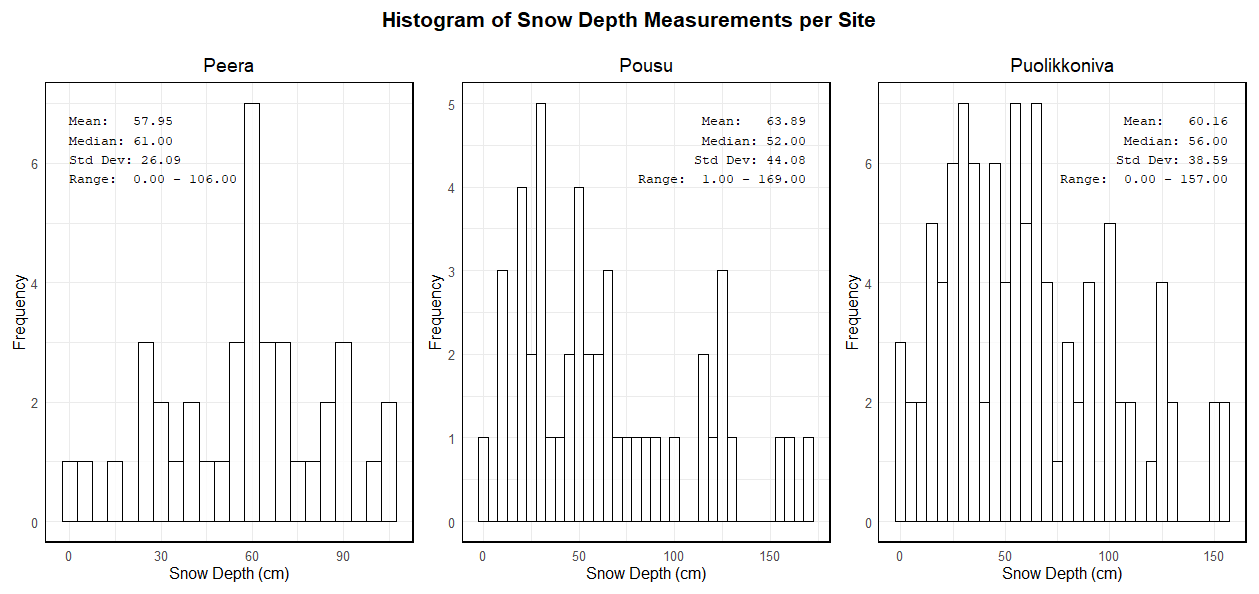
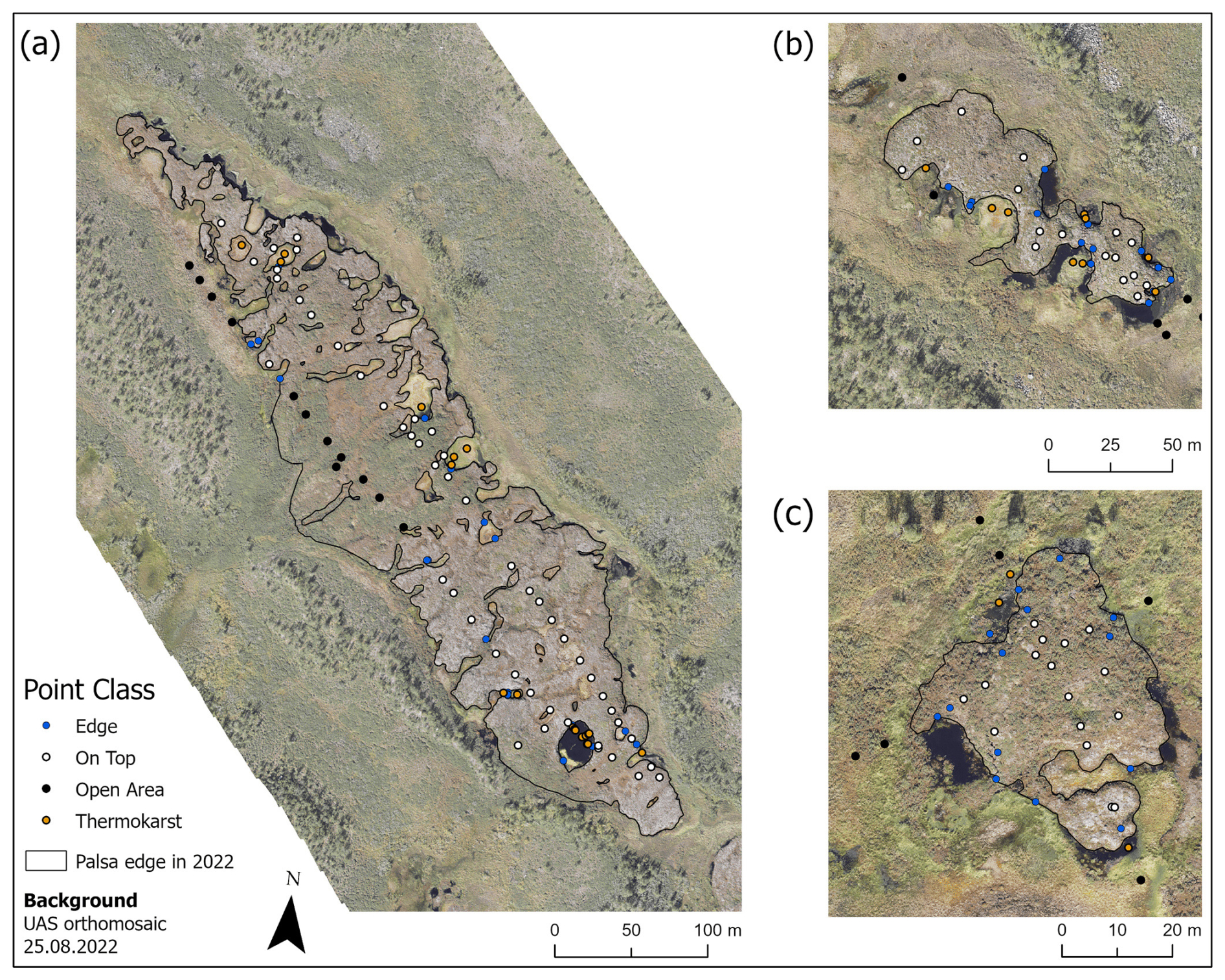
Figure A2 Overview of the classification of all SD_{in situ} points into the edge, on-top, open-area and thermokarst classes.

Table A1 Correlation between each input parameter and RF-modelled snow depth.