Drift-aware sea ice thickness maps from satellite remote sensing

The standard approach to deriving gridded sea ice thickness (SIT) from satellite altimeters is to aggregate the original along-track SIT estimates over a 1-month period to achieve sufficient coverage across the Arctic. However, this approach neglects processes like sea ice advection, deformation, and thermodynamic growth that occur within the aggregation period. To address these limitations, we propose a drift-aware method that accounts for sea ice motion and SIT changes due to dynamics and thermodynamics in monthly SIT products. We present a method to derive daily drift-aware sea ice thickness (DA-SIT) maps for the Arctic based on Envisat and CryoSat-2 along-track data. The approach is validated against buoys, airborne SIT surveys, and moored upward-looking sonar (ULS) measurements. DA-SIT demonstrates the ability to register sea ice thickness anomalies, which are also observed by daily ULS SIT averages but are overlooked by the conventional gridded SIT data. Comparative analysis reveals that drift awareness reduces orbit track patterns in the gridded SIT and improves consistency in regions with significant ice drift, such as the transpolar drift. The drift awareness facilitates detailed studies of regional sea ice dynamics and fluxes, while improving co-registration of multi-mission satellite data. However, when considering pan-Arctic estimates of ice volume, we do not expect significant changes in time series and trends compared to in existing studies.

1 Introduction

The polar regions are a hot spot of climate change, associated with rising air temperatures (Landrum and Holland, 2020) and the transition of the Arctic Ocean to a state similar to Atlantic waters, a process known as Atlantification (Polyakov et al., 2017). As a consequence, Arctic sea ice has significantly declined during the last decades, in both summer extent and year-round thickness (Comiso et al., 2008; Lindsay and Schweiger, 2015; Ricker et al., 2021). To monitor sea ice decline on a large scale, satellite observations are crucial. Observing sea ice thickness (SIT) is important as its magnitude regulates the heat exchange between ocean and atmosphere. In fact, SIT is an essential climate variable (ECV) quantity (Lavergne et al., 2022) and is critical for the calculation of sea ice volume and mass balance (Bocquet et al., 2024; Heorton et al., 2025), as well as freshwater fluxes (Ricker et al., 2018; Selyuzhenok et al., 2020).

Satellite altimetry has become the major tool for estimating SIT (Laxon et al., 2013; Ricker et al., 2014; Tilling et al., 2018; Petty et al., 2020). Within the European Space Agency (ESA) Climate Change Initiative (CCI), consistent SIT time series are developed across multiple satellite radar altimetry missions (ERS, Envisat, CryoSat-2, and Sentinel-3) to observe long-term trends (Paul et al., 2018). However, existing methods for producing monthly SIT maps are hindered by the fact that the sea ice is constantly in motion (Spreen et al., 2011), primarily driven by winds and, to a lesser extent, ocean currents. With the standard approach, along-track SIT estimates derived from satellite altimetry measurements are typically collected over 1 month, allowing for equal-orbit coverage of the polar regions (Sallila et al., 2019). SIT is then averaged onto a fixed grid, where each input SIT estimate is geolocated at the time of the original measurement. Other methods use more advanced interpolation techniques, such as optimal interpolation or Bayesian approaches (Ricker et al., 2017; Gregory et al., 2021). All these approaches neglect sea ice drift occurring within the data collection period and, therefore, introduces uncertainties into the final SIT maps. This is also important in the context of increasing sea ice drift speed over the last decades, and studies suggest that sea ice mobility will further increase in the future (Kwok et al., 2013; Zhang et al., 2022). Within the transpolar drift or Fram Strait, the geodesic displacement of sea ice can reach several hundred kilometers within a month (Kwok et al., 2004; Lavergne and Down, 2023). In addition to the advection of sea ice, deformation and thermodynamic ice growth occur within the data collection period of 1 month, meaning that SIT of a certain parcel derived at the beginning of a month will be altered by the end of the collection period. Moreover, because the temporal distribution of satellite orbits is uneven across regions throughout the month, the uncertainty associated with SIT changes will vary spatially.

As sea ice drift increases, advances in satellite altimetry, such as the laser altimeter on the NASA Ice, Cloud, and land Elevation Satellite 2 (ICESat-2), enable the detection of fine-scale features like individual sea ice pressure ridges (Farrell et al., 2020; Ricker et al., 2023). However, without accounting for sea ice motion, much of this detail can be lost when applying standard gridding techniques to generate SIT maps.

When retrieving geophysical information from multi-platform datasets, such as ice thickness from CryoSat-2 and the Soil Moisture and Ocean Salinity satellite (SMOS) (Ricker et al., 2017), correcting for ice motion prior to data merging is a step toward improving accuracy. Another example is the CRYO2ICE campaign (Fredensborg Hansen et al., 2024) to observe snow depth on sea ice by combining CryoSat-2 radar and ICESat-2 laser altimeter measurements, which currently relies on single-synchronized orbits due to sea ice drift.

To reduce uncertainties in SIT maps due to sea ice drift, we propose a novel approach that incorporates sea ice drift estimates from passive microwave satellite radiometers and combines them with satellite altimetry data to derive drift-aware sea ice thickness maps. This method allows individual parcels of satellite altimeter measurements to be advected over time, correcting for motion while also capturing sea ice thickness change as a consequence of thermodynamic growth and deformation effects between satellite overpasses.

Therefore our objective is to describe the drift-aware sea ice thickness (DA-SIT) algorithm based on data from Envisat (2002–2012) and CryoSat-2 (2010–2020). In addition, our goal is to validate and benchmark DA-SIT using drifting buoys, airborne sea ice thickness surveys, and moored upward-looking sonars (ULSs) while assessing the impact of the drift-awareness algorithm by a comparison with conventionally gridded sea ice thickness products. In particular, we will show that neglecting sea ice drift causes significant spatial blurring and nonuniform temporal coverage in general, compromising the accuracy of regional thickness distributions.

This paper is outlined as follows: in the first part in Sect. 2, we describe the individual input datasets, while in the second part, we describe the drift-aware processing algorithm, including the estimation of associated uncertainty. In Sect. 3, we present the results from the DA-SIT evaluation against independent validation datasets. In Sect. 4, we explore the impact of DA-SIT. Finally, conclusions are drawn in Sect. 5.

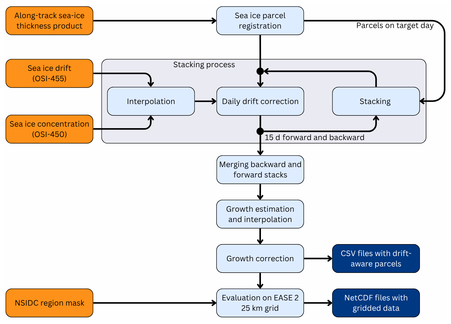
Figure 1 Drift-aware sea ice thickness processing flow chart. Orange boxes indicate input data, light-blue boxes indicate processes, and dark-blue boxes indicate output data products.

2 Data and methods

2.1 Input data

2.1.1 Altimeter datasets

We have chosen to demonstrate the drift-awareness algorithm on SIT retrievals, as they are most relevant for further scientific studies, but it is equally relevant for freeboard and other geophysical information obtained from altimetry.

As this study is related to the ESA CCI project, we use the latest CCI climate data record version 3.0 of SIT for the Northern Hemisphere polar region. The drift-awareness input altimetry dataset contains the along-track geophysical variables, including SIT and the corresponding point-wise geolocation information (longitude, latitude), which is typically classified as a level-2 dataset. Additional variables such as snow depth and freeboard are tracked along with the SIT data. The dataset includes two satellite missions. From October 2002 to March 2012, we use daily along-track SIT data from the Radar Altimeter-2 (RA-2) instrument on the Envisat satellite. From November 2010 to April 2020, we use daily SIT data from the satellite radar altimetry (SAR) Interferometer Radar Altimeter (SIRAL) instrument aboard CryoSat-2. Both datasets cover the winter months (October to April) and are provided at a full sensor resolution (Hendricks et al., 2024a, b). For a detailed description of the CCI along-track SIT retrieval processing, see Paul et al. (2024). This study is a proof of concept for single-altimeter data and is in principle applicable to other platforms, such as ERS-2, Sentinel-3, and ICESat-2.

2.1.2 Sea ice concentration

For sea ice concentration, we use the Ocean and Sea Ice Satellite Application Facility (OSI SAF) Global Sea Ice Concentration Climate Data Product (CDR) version 3 (OSI-450-a, 2022), which covers the period of 1978–2020 and is routinely extended by the Interim CDR OSI-430-a. OSI-450-a is a full reprocessing of sea ice concentration, using improved algorithms and an upgraded processing chain (Lavergne et al., 2023, 2019). Sea ice concentration is obtained from passive microwave radiometer data, including the scanning multi-channel microwave radiometer (SMMR), the special sensor microwave/imager (SSM/I), and the special sensor microwave imager/sounder (SSMIS), as well as ERA5 reanalysis data. Ice concentration is provided on daily EASE2 grids with a spatial resolution of 25 km.

2.1.3 Sea ice drift

For sea ice drift, we use the OSI SAF low-resolution Global Sea Ice Drift CDR version 1 (OSI-455, 2022), which covers the period of 1991–2020. OSI-455 provides displacements over a time span of 24 h on a 75 km grid and is based on passive microwave radiometer data, including the satellite sensors SSM/I and SSMIS, the advanced microwave scanning radiometer for Earth Observing System (AMSR-E), and the advanced microwave scanning radiometer 2 (AMSR2). Displacements are estimated using a cross-correlation method on pairs of satellite images. OSI-455 builds on the methodologies of the near-real-time sea ice drift product OSI-405 (OSI-405, 2007). More details about the algorithm used can be found in Lavergne and Down (2023). If data on individual days are missing, the data product of the closest day available is used. OSI-455 also provides uncertainty estimates (1 standard deviation) for the dX and dY components of the drift vector, which are used for the DA-SIT uncertainty estimation.

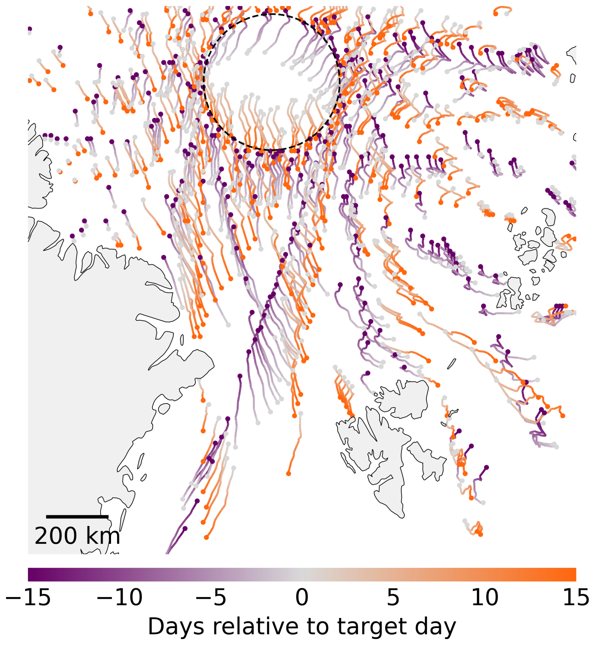
Figure 2 Every 10th sea ice parcel trajectory with origins at the beginning or end of March 2020 and the target day on the 15th of March. The dashed black circle at 88° N marks the CryoSat-2 pole hole.

Figure 3 Processing scheme to produce the DA-SIT product. Each cell represents sea ice observations from 1 d. The color map and vertical axis represent the delay regarding the time of data acquisition. The horizontal axis represents the ordinary timeline in days; e.g., day 0 may represent 1 October, and day N refers to 30 April. Diagonally aligned boxes (lower left to upper right for forward projection) represent daily trajectories, which are drift corrected daily, containing the same SIT data from the day of acquisition.

2.2 Drift-aware sea ice thickness trajectories

Figure 1 shows the processing scheme for the drift-aware sea ice thickness (DA-SIT) product. The processing is divided into several steps, which are executed sequentially for each winter season. In the following, we describe the individual steps required to compute DA-SIT, corresponding to Fig. 1.

2.2.1 Sea ice parcel registration

In the first step, the along-track SIT data products (Envisat, CryoSat-2) are collected on a daily basis. For the sea ice parcel registration, these individual data points are aggregated within circular parcels with a radius of $R=\sqrt{\mathrm{2}}\cdot \mathrm{10}$ km. This registration in parcels is done to reduce the computational costs of the drift correction step. The parcel-wise tracking is also justified, considering the coarse spatial resolution of the drift product (see Sect. 2.1.3).

The location of parcel centers is selected using the National Snow and Ice Data Center (NSIDC) EASE-Grid 2.0 (Brodzik et al., 2012) with a spacing of 10 km in both the x and y directions. The chosen radius ensures partial overlap between parcels, improving the robustness of SIT distribution representation and mitigating geolocation errors.

Parcels are initially registered using the centroid of each grid cell, corresponding to the central position of each circular polygon. The mean SIT is calculated for each parcel. To ensure the presence of sea ice, the OSI-450-a sea ice concentration product is interpolated onto the initial parcel positions. Parcels with a sea ice concentrations below 15 % are excluded from the following processing steps.

2.2.2 Drift correction

The drift correction is applied to parcels both forward and backward in time on a daily basis. The day onto which parcels are projected by applying the drift correction is called the target day. The OSI-455 displacements are first resampled onto the sea ice concentration grid and then interpolated onto parcel positions with a minimum sea ice concentration of 15 % using a bi-linear interpolation scheme.

The time bounds of the OSI-455 drift product span 12:00 UTC on the previous day to 12:00 UTC on the day corresponding to the dataset registration time. The latter (12:00 UTC of the registration day) also serves as the reference time for the daily DA-SIT. Consequently, to correct drift on a given day, we use the drift product associated with a reference time set 1 d in advance.

For the initial drift correction of parcels, we first calculate the time difference between the registration time of the sea ice parcel on the target day and the reference time of the drift product (12:00 UTC 1 d ahead). This difference is typically close to 24 h. Using this time difference, we adjust the position of the sea ice parcel accordingly. Following this correction, the reference time for all parcels is standardized to 12:00 UTC of the respective day. Subsequent drift corrections involve a consistent 24 h displacement. We use a first-order Runge–Kutta integration scheme, equivalent to Euler's method. While a fourth-order scheme generally offers higher accuracy, it comes with significantly greater computational cost. Given that the drift vectors are defined on a 75 km grid and daily displacements are significantly smaller than this resolution, a higher-order scheme was not implemented.

Next, we use the OSI-450-a ice concentration corresponding to the day when the parcel reaches its updated position. Ice concentration is interpolated onto these updated positions, and any parcels located in areas with ice concentration below a threshold of 15 % are removed, as we assume that ice drifting into the open ocean will melt even during polar winter. Therefore, these parcels are removed from the dataset. We also ensure that parcels do not unintentionally drift onto land grid cells, which can occasionally occur due to the low resolution of the drift product and related uncertainties.

As a result of the systematic drift correction, the original along-track SIT pattern disperses, transforming into a point cloud where each point represents a circular parcel. This process is repeated daily, progressively updating the positions of the parcels over time. This dispersion is illustrated in Fig. 2. The map shows a selection of parcel trajectories with a length of 15 d. The parcels originate either 15 d prior to or 15 d after the target day. While the parcels initially align with the satellite’s track pattern, after 15 d they can drift by over 200 km in some cases.

2.2.3 Stacking process

The stacking scheme is illustrated in Fig. 3. Processing typically begins on 1 October (day 0), the first day after the summer pause when altimetry processing resumes. On this day, sea ice parcels are initially registered following the procedure described in Sect. 2.2.1. The drift correction, as outlined in Sect. 2.2.2, is then applied to these parcels. Each elapsing day, newly registered parcels or parcels already corrected for drift on the previous days are advected. For each parcel, a maximum of 15 daily drift corrections is allowed. Parcels are removed from the stack after the 15th correction.

This procedure is performed in both forward and backward time directions. Each day, drift-corrected parcels are stacked onto the drift-corrected parcels from 1 d prior or 1 d ahead, depending on the direction. A set of parcels is organized in a data frame structure, which contains the parcel geometries and their trajectories from the initial registration until the end of the drift (nominally 15 d).

The trajectory of each parcel is represented as a list of points, beginning with its initial registration position and ending at its final drift-corrected destination. Forward-projected parcels have trajectories progressing forward in time, while backward-projected parcels have trajectories moving backward in time.

As shown in Fig. 3, starting with a set of parcels on day 0, the process produces a stack of 31 parcel sets by day 15. This includes 15 sets from forward projections, 15 from backward projections, and the initial parcel set derived from the along-track SIT product on the target day. The diagonals in Fig. 3 represent the same parcels (and therefore the same SIT data) but at varying positions within the space–time domain due to daily forward or backward drift corrections. Ultimately, the vertically stacked parcel sets, spanning both past and future days, represent the predicted parcel positions on the target day.

After completing the forward and backward stacking, the parcel sets within a single stack are merged to create the drift-corrected dataset for a given target day (Fig. 3). Specifically, the parcel sets are combined into a unified data frame. Since both the forward and backward stacks include the parcel set corresponding to the target day, one of these is removed to prevent duplication.

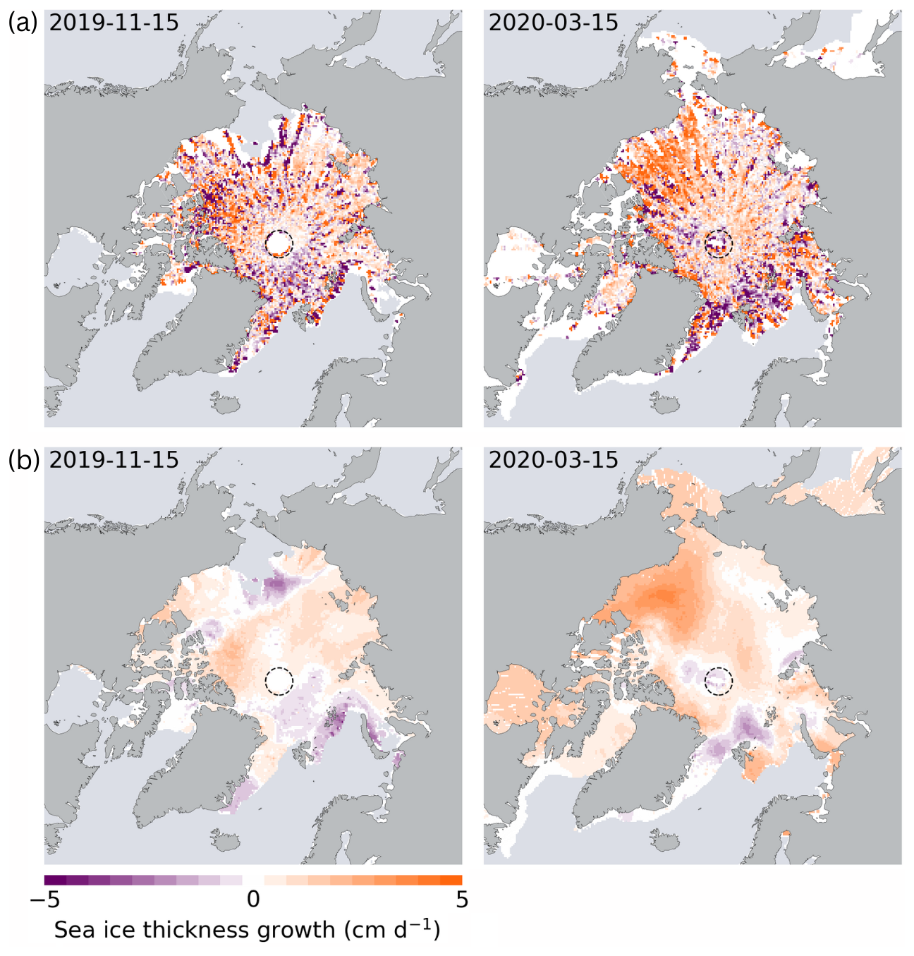
Figure 4 (a) Sea ice growth estimates from CryoSat-2 across the Arctic for November 2019 and March 2020 within a full stack of parcel sets covering 1 month. (b) Spatially interpolated sea ice growth based on the growth estimates shown in (a). The white area in the background indicates data gaps with respect to the actual ice extent. The dashed circle represents the pole hole of the CryoSat-2 orbit coverage.

2.2.4 Growth estimation and correction

Growth estimation aims to correct the SIT of parcels for processes that alter the thickness along their space–time trajectory. While parcels are drift-corrected, their SIT remains fixed at the state of initial registration. However, dynamic and thermodynamic processes alter the thickness between the registration time and the target day, which is typically up to 15 d. To account for these changes, we make use of the drift-corrected ice parcels. The drift correction ensures that parcels, which are collocated in space but with different registration times, represent a snapshot of the same ice regime, observed at different times. This allows us to apply a linear-growth model.

In the initial step of the growth correction process, we create a 25×25 km EASE2 grid. Next, we assign all parcels from the full stack to their corresponding grid cells. When a grid cell contains at least three parcels with SIT estimates from different points in time, we apply a least-squares linear fit:

$$\begin{array}{}\text{(1)}& f_H\left(n\right)=p_{\mathrm{1}}n+p_{\mathrm{0}},\end{array}$$

where f_H is the fitted sea ice thickness, and n represents the number of days between the day of measurements and the target day. p₀ is the projected SIT on the target day. The coefficient p₁ represents the SIT growth, which can be positive or negative. It is important to note that, at this stage, we do not differentiate between thermodynamic and dynamic growth processes. Additionally, we acknowledge that due to uncertainties in the drift product and nonuniform altimeter measurement coverage within parcels, exact spatial collocations are unlikely. Nonetheless, we assume that SIT values are representative within a given area, chosen here to be 25×25 km, which is smaller than the typical SIT correlation lengths in the Arctic (Ricker et al., 2017). Therefore, this method is representative of average ice thickness at grid resolution scale, neglecting thickness variations between individual sea ice floes. The linear fitting generates a covariance matrix, which quantifies the uncertainty in p₁. This uncertainty is later used for the overall uncertainty estimation. Figure 4a illustrates an example of gridded growth estimates derived from a stack of trajectories centered on 15 November 2019 and 15 March 2020. These estimates represent ice growth over 1-month periods. The density of growth estimates across the Arctic decreases with latitude as the orbit density decreases. Therefore, uncertainties in these estimates increase with distance from the pole. In some regions, very high and very low growth rates appear side by side, and overall, the gridded growth estimates exhibit considerable noise. This is partly because the linear fit is highly sensitive to abrupt changes in SIT, which may occur naturally or result from measurement uncertainties. Such variability can introduce significant noise or bias into the estimated growth rates. Additionally, the SIT estimates used for the fit are obtained over differing time intervals, leading to inconsistencies in temporal resolution. These inconsistencies can degrade the stability of the fitted growth estimates.

To achieve a consistent growth correction, we fill the gaps that are left when not enough collocated parcels from different times could be identified. Here we use a radial basis function (RBF) interpolation in two dimensions with a Gaussian kernel based on the scipy.interpolate.RBFInterpolator function (Virtanen et al., 2020). An RBF interpolant based on data values d at locations y is a linear combination of RBFs centered on y and a polynomial P(x) of a specific degree, evaluated at position x (Virtanen et al., 2020):

$$\begin{array}{}\text{(2)}& f\left(x\right)=K(x,y)a+P\left(x\right)b,\end{array}$$

where K(x,y) is an array of RBFs centered on y and evaluated at x. The coefficients a and b solve the following linear equations:

$$\begin{array}{}\text{(3)}& {\displaystyle }\left(K(y,y)+\mathit{\lambda }\left(\mathrm{\Phi }\right)I\right)a+P\left(y\right)b=d\text{(4)}& {\displaystyle }P(y{)}^{T}a=\mathrm{0}.\end{array}$$

Here, λ(Φ) is a smoothing-scale parameter chosen to be latitude-dependent to account for the varying density of measurement points caused by the satellite's orbital geometry. The smoothing-scale parameter decreases linearly from 80 at Φ=40° N to 10 at Φ=90° N. For further details on the RBF interpolation method, we refer to Virtanen et al. (2020).

To minimize computation time, we limit the number of nearest data points used for each interpolation to a maximum of 260. Figure 4b illustrates an example of spatially interpolated sea ice growth for 15 November 2019 and 15 March 2020. The interpolated ice growth values are then applied to adjust the SIT estimates of the parcels, considering the number of days between the actual measurement date and the target day. Finally, parcel trajectories aggregated over 1 month are exported in daily comma-separated value (csv) files (Fig. 3).

2.2.5 Computing performance

The computing efficiency of the stacking process benefits from parallel processing, which is implemented in the DriftAware-SIAlt Python software. On a high-performance computing cluster (HPC) using 16 CPU cores and 8 GB memory per CPU, the processing of csv files with DA trajectories for an entire winter season (October–April) takes approximately 4 h. A set of daily csv files containing the DA trajectories for one winter season requires approximately 30 GB, with individual file sizes between 40 and 170 MB.

Figure 5 Drift-aware sea ice thickness from Envisat (2002/2003) and CryoSat-2 (2019/2020) for November and March with applied sea ice growth correction. The white area in the background indicates data gaps with respect to the actual ice extent. The dashed circle represents the pole hole of the Envisat/CryoSat-2 orbit coverage.

2.3 Evaluation on the EASE2 grid

We evaluate the stacked, SIT-growth-corrected parcel sets on a 25 km EASE2 grid, in line with other existing SIT products (e.g., Ricker et al., 2017) and with the SIC climate data record. We average the SIT of the parcel sets at their positions on the respective target days within 25 km grid cells. This means we will retrieve daily DA-SIT grids, each containing data from a monthly window (15 d in both directions). Therefore, to provide gridded products that contain entirely independent data, we must consider the daily stacks with a 1-month difference in reference time. To align with the conventional monthly gridded products, we select the mid-month stacks to compute the respective DA-SIT grids, i.e., on the 15th of each month. During the ramping phase in the beginning and end of the processing period, stacks are not full and, therefore, gridded maps will be incomplete within the first and last 15 d of the processing period (Fig. 3).

The average SIT (H_L3) for one grid cell is computed as an arithmetic mean, ignoring non-numeric values:

$$\begin{array}{}\text{(5)}& H_{L\mathrm{3}}={\displaystyle \frac{\mathrm{1}}{n_{L\mathrm{2}}}}\cdot \sum _{i=\mathrm{0}}^{n_{L\mathrm{2}}}{H}_{i,L\mathrm{2}}\text{ if }{H}_{i,L\mathrm{2}}\ne \text{NaN},\end{array}$$

where n_L2 is the number of parcels inside the corresponding grid cell.

Figure 5 shows the final gridded DA-SIT for Envisat (November 2002 and March 2003) and CryoSat-2 (November 2019 and March 2020) after SIT growth correction. The drift correction can cause parcels to slide into the pole hole, reducing its size. But the drift awareness can also result in data gaps like in the Chukchi Sea in November 2002. Those gaps arise when the satellite's orbital drift aligns in both direction and magnitude with the drift of the sea ice. In fact, this means that DA-SIT also reveals sea ice areas that have never been surveyed by the satellite within the 1-month observation period.

Figure 6 (a) Uncertainty components of the Envisat DA-SIT product for 15 March 2003. (b) Uncertainty components of the CryoSat-2 DA-SIT product for 15 March 2020. The white area in the background indicates data gaps with respect to the actual ice extent. The dashed circle represents the actual pole hole of the Envisat/CryoSat-2 orbit coverage.

2.4 Uncertainties

We distinguish between three major contributors to uncertainties in the gridded DA-SIT.

1. The uncertainty associated with the along-track SIT retrieval, used as input for drift-aware processing, is derived from the level-2 along-track SIT of the CCI climate data record version 3.0.

   The uncertainty in the mean SIT (${\mathit{\sigma }}_{H_{\mathrm{parcel}}}$) for each parcel is computed by considering the individual uncertainties in measurements associated with the parcel:

   $$\begin{array}{}\text{(6)}& {\mathit{\sigma }}_{H_{\mathrm{parcel}}}={\displaystyle \frac{\sqrt{{\sum }_{i=\mathrm{1}}^n{\mathit{\sigma }}_i^{\mathrm{2}}}}{n}},\end{array}$$

   where σ_i represents the uncertainty associated with the ith measurement, and n is the total number of measurements. This calculation assumes that the uncertainties are uncorrelated.

2. The uncertainty in SIT as a consequence of the drift uncertainty depends on two factors: first, the uncertainty in the ice drift product and, second, the spatial variability in SIT in the area that the parcel might have drifted into, considering the drift uncertainty. We start with aggregating the drift uncertainty along the parcel trajectory. In OSI-455, the daily drift uncertainty estimates, σ_D, are identical in both the x and y directions. For each step of drift correction, the squares of the drift uncertainties are aggregated. After the final drift correction, the drift uncertainty, ${\mathit{\sigma }}_{{\text{D}}_{x,y}}\left(t_j\right)$, of a parcel at the target day t_j is computed as follows:

   $$\begin{array}{}\text{(7)}& {\mathit{\sigma }}_{{\text{D}}_{x,y}}\left(t_j\right)=\sqrt{\sum _{i=j-N}^j{\left({\mathit{\sigma }}_{{\text{D}}_{x,y}}\left(t_i\right)\right)}^{\mathrm{2}}},\end{array}$$

   where N is the number of days over which drift correction is performed (up to 15 d), t_j represents the time of the target day assigned the index j, and i represents the day of data acquisition (the starting point of the drift). In the second step, we analyze the impact of the spatial SIT variability. After the merging of forward and backward stacks, including growth correction (Sect. 2.2.3 and 2.2.4), all neighboring ice parcels within the area defined by the drift uncertainty are aggregated at each parcel's final position. The aggregation uses a radius defined as $\sqrt{\mathrm{2}}{\mathit{\sigma }}_{{\text{D}}_{x,y}}\left(t_j\right)$, where ${\mathit{\sigma }}_{{\text{D}}_{x,y}}\left(t_j\right)$ represents the estimated uncertainty in the x and y directions.

   This results in a SIT distribution over the area where the ice parcel may have drifted, accounting for the drift uncertainty. If the thickness in this area is highly homogeneous, significant uncertainties in SIT are not expected, as the varying position of the ice parcel will not alter the SIT distribution within the area. Conversely, if the SIT in this area is highly heterogeneous, with substantial gradients, a different position of the ice parcel could result in changes to the SIT at its location. To estimate the potential uncertainty in SIT within the drift uncertainty radius, we calculate the interquartile range of the SIT distribution in that area, defined as the difference between the 75th and 25th percentiles. However, if the drift uncertainty radius does not exceed the radius of the parcel area, the resulting SIT uncertainty is set to 0. This is the case for fastened sea ice in particular.

3. The uncertainty due to SIT growth and its correction is estimated from the covariance matrix obtained through linear fitting, which is used to estimate SIT growth (Sect. 3.6). For each parcel's growth estimate, the growth uncertainty, ${\mathit{\sigma }}_{H_{\text{G}}}$, is computed as follows:

   $$\begin{array}{}\text{(8)}& {\mathit{\sigma }}_{H_{\text{G}}}\left(\mathrm{\Delta }t\right)=\sqrt{{\mathit{\sigma }}_{p_{\mathrm{1}}}^{\mathrm{2}}}\mathrm{\Delta }t,\end{array}$$

   where ${\mathit{\sigma }}_{p_{\mathrm{1}}}^{\mathrm{2}}$ is the variance term of the growth coefficient p₁, derived from the diagonal elements of the covariance matrix. p₁ is multiplied by the time difference Δt, measured in days, between the target day and the day of data acquisition to calculate the SIT uncertainty due to ice growth for a given ice parcel.

The total uncertainty is calculated by the square root of the sum of the squares of the three individual components. Figure 6 shows the three uncertainty components as well as the total uncertainty in DA-SIT for Envisat (15 March 2003) and CryoSat-2 (15 March 2020). The along-track SIT uncertainty is relatively uniform across the central Arctic but larger along the coastlines and over thinner ice (Ricker et al., 2017). Moreover, the pulse-limited RA-2/Envisat radar measurements generally cause higher along-track sea ice thickness (SIT) uncertainty compared to that in CryoSat-2. The SIT uncertainty caused by ice drift is significantly smaller in the pack ice but becomes more pronounced in the marginal ice zone and especially along coastlines. This is primarily due to the greater uncertainty in drift products near coastlines, whereas the relatively low drift uncertainties in the pack ice zone often result in accumulated displacement uncertainties that remain smaller than the radius of the sea ice parcel cell. It is also worth noting that examples from recent years benefit from the AMSR2 mission, which started in 2012. Earlier years, dominated by the SSM/I missions, may exhibit larger drift-related uncertainties. More information on the ice drift uncertainties is provided in Lavergne and Down (2023) and Sumata et al. (2014). The SIT uncertainty due to ice growth shows a distinct orbital pattern, a result of the growth uncertainty being a function of the time elapsed between the data acquisition and target day. The total uncertainty pattern is, therefore, a superposition of the patterns of the individual components.

Figure 7 (a) Validation of DA trajectories with buoys, including example trajectories (T1-4). Green-filled circles represent the DA uncertainty in the drift correction after ±15 d. (b) Distance between DA-SIT and the buoy trajectory after 3, 8, and 15 d as a function of DA path length. (c) Yearly mean distance between DA and the buoy trajectory after 3, 8, and 15 d in both directions.

3 Validation of the drift-aware sea ice thickness

3.1 Validation of DA-SIT trajectories using buoys

We use trajectories from autonomous buoys to validate the DA-SIT trajectories. We use buoy data provided by the International Arctic Buoy Program (IABP). The IABP includes different types of buoys that measure snow and ice parameters such as ice temperature, snow depth, and SIT. However, for this study, we only use the buoy positions. Although IABP also includes ice mass balance buoys to measure sea ice thickness, we do not use them for the SIT evaluation, as their measurements only represent the sea ice at their immediate position, and they are therefore not suited for comparing with satellite observations, which require the integration of SIT measurements over at least several hundred meters. In total we use 1029 buoys. The original sampling frequency of the buoy data was 3-hourly until 2016 and hourly thereafter. We resample the IABP buoy data to daily positions at 12:00 UTC to align with the reference time of the DA-SIT trajectories. The daily buoy positions are then divided into 31 d periods, centered on a target day with a ±15 d window to align with the DA-SIT trajectories. For the starting dates of the 15 d buoy trajectories, we identify the spatially closest initial DA-SIT ice parcels from all available trajectories. This includes trajectories in both the forward and backward directions. We set a maximum distance threshold of 25 km between the buoy and the initial DA-SIT ice parcel position. This threshold is well below the spatial resolution of the drift product, minimizing any significant impact of positional offsets between the initial positions of the parcel and the buoys.

Figure 7a shows a map of distances between the end points of individual DA-SIT trajectories and the corresponding buoy trajectories. We consider only the distances after 15 d of drift, either backward or forward in time. The pattern indicates higher uncertainties in the DA-SIT trajectories in the Fram Strait and East Greenland Sea as well as in the marginal ice zones and in peripheral locations. Here, the discrepancy after 15 d of drift correction can reach more than 50 km. In contrast, the central Arctic shows distances of typically less than 10 km, which is below the grid-cell size.

Figure 7b shows the linkage between the uncertainty in the DA-SIT trajectory and the path length. The path length is the distance covered along the trajectory. It begins on the day of the measurements and ends on the target day and generally increases with time. With increasing time lag and path length, the distance between buoy location and DA ice parcel location is also increasing. After 3 d, we observe a median distance of 2.77 km, considering all co-registered trajectories, but it increases to 6.57 km after 15 d. Therefore, we conclude that with increasing DA time lag, the uncertainty in the respective ice parcel location increases. This uncertainty is described in Sect. 2.4 and displayed in the four trajectory examples in Fig. 7a. Figure 7c shows the yearly mean distance between the DA-SIT parcel and buoy location for all co-registered trajectories across the Arctic after 3, 8, and 15 d. There is no significant trend in the distances between the buoy and DA ice parcel within the 2002–2020 period. We also do not observe a significant difference in the distances between backward- and forward-projected trajectories. However, as discussed before (Fig. 7b), we observe a dependency of the distance on the time lag. The longer the time lag between the target day and the day of measurements, the higher the discrepancy between the buoy and DA-SIT parcel locations.

Figure 8 (a) Overview of DA-SIT validation data across the Arctic. Airborne electromagnetic thickness sounding (AEM) surveys are sorted by year. The black stars indicate the locations of the ULS (Beaufort Gyre Exploration Project – BGEP – moorings). (b) Box-and-whisker plots of total DA-SIT and conventionally gridded SIT (separated between the Envisat and CryoSat-2 eras) plotted against binned AEM total sea ice thickness. Gray dots in the background represent the actual distribution. The scaled circles below the box-and-whisker plots indicate the number of points in each bin. The bin width is 0.5 m.

3.2 Validation with airborne EM

Airborne electromagnetic induction thickness sounding (AEM) is a method to measure total sea ice thickness directly. The EM-Bird is an AEM sensor that is towed over sea ice by a helicopter or fixed-wing aircraft (Pfaffling et al., 2007; Haas et al., 2009). The distance to the sea ice–seawater interface is calculated from the EM response. The sea ice–snow–air interface is obtained from a laser altimeter. The difference between the two interfaces corresponds to the sea ice and snow thickness. The point spacing of the measurements is approximately 5 m.

We use AEM data from helicopter and fixed-wing aircraft campaigns during the period of 2007–2019 (Table A1). AEM data are projected and averaged on a 25 km EASE2 grid in line with the gridded DA-SIT. Since the AEM data represent total thickness, which combines SIT and snow depth, we need to convert the DA-SIT estimates accordingly. In the drift-aware processing, the snow depth from the along-track data is assigned to parcels in the same way as SIT and is therefore also drift-corrected. Consequently, we add the gridded snow depth to the DA-SIT retrieval in order to obtain the DA total thickness. Daily grids of AEM data are then compared with the matching DA-SIT grids. The validation of the gridded DA-SIT product against total ice thickness is carried out for both the Envisat and the CryoSat-2 eras and allows us to evaluate the spatial distribution of SIT at a given time. Due to the larger Envisat pole hole (>81.4° N), suitable AEM surveys are primarily limited to the Beaufort and Chukchi Sea (Fig. 8a). Therefore, the surveyed ice does not contain ice as thick and deformed as in the Lincoln Sea, for example. The CryoSat-2 orbit domain extends up to 88° N and thus also includes AEM surveys over thick, deformed multi-year sea ice. Figure 8b shows validation results for each satellite era. The bias is −0.61 m for Envisat and −0.13 m for CryoSat-2. The root-mean-square deviation (RMSD) is comparable between the two sensors, measuring 0.89 m for Envisat and 0.98 m for CryoSat-2. The Pearson correlation differs significantly, with a value of r=0.68 for CryoSat-2 and only r=0.13 for Envisat. The weak correlation and slight underestimation of thickness observed in the Envisat data can be attributed to the limitations of its pulse-limited altimeter type, which lacks the ability to adequately capture deformed sea ice (Paul et al., 2018). For reference, Fig. 8b also shows the total sea ice thickness derived from conventional gridding (C-SIT), which does not include drift awareness but uses the same gridding scheme (Sect. 2.3). For C-SIT, parcel positions are taken at the time of the satellite overflight and are gridded by aggregating data within a daily shifting 1-month time window. The comparison between DA-SIT and C-SIT with regard to the validation with AEM reveals only minor differences. This suggests that the effect of drift awareness is mostly overruled by other sources of uncertainty such as the limitations due to the satellite footprint in contrast to the high-resolution airborne measurements. The direct comparison between DA-SIT and C-SIT is discussed in Sect. 4 in more detail.

Figure 9 (a) Box-and-whisker plots of daily DA draft and conventionally gridded ice draft (Envisat 2002–2012, CryoSat-2 2010–2020) plotted against binned daily averaged ULS draft. Gray dots in the background represent the actual distribution. The scaled circles below the box-and-whisker plots indicate the number of points in each bin. The bin width is 0.25 m. (b) Daily sea ice draft from ULS and the co-registered DA draft as well as ice draft from conventionally gridded SIT over the winter seasons 2008/2009 (CryoSat-2) and 2018/2019 (CryoSat-2).

3.3 Validation with ULS

Upward-looking sonars (ULSs) are mounted on oceanographic moorings (Hansen et al., 2013; Krishfield et al., 2014) and provide information on long-term ice thickness variability and seasonal changes. ULSs are used to derive ice draft by measuring the travel time of a sonar pulse transmitted by the ULS and reflected back from the ice bottom. The ice draft can then be converted into ice thickness, assuming snow load and densities of snow and ice. In contrast to AEM, ULSs are valuable to evaluate the temporal change in sea ice draft in the vicinity of the ULS location. We use ULS ice draft data from moorings that have been deployed at four different sites in the Beaufort Sea within the Beaufort Gyre Exploration Project (BGEP, Krishfield et al. (2014)). Figure 8a shows the position of the moorings in the Beaufort Sea. Their draft time series cover the Envisat (A, B, C, D) and the CryoSat-2 eras (A, B, D). Exact locations and data record periods for the ULS A–D are provided in Table A2.

The original data are sampled at 2 s intervals. We first remove open-water sections. Afterwards, the filtered data were averaged over 24 h to obtain daily mean effective ice thickness for each ULS. Then, for each day and each ULS position, we co-register the nearest three grid cells in the DA-SIT grids. The thicknesses and uncertainties in the three grid cells are averaged. As the ULSs provide draft estimates, we convert the co-registered DA-SIT into ice draft using climatological densities for ice (900 kg m⁻³), snow (300 kg m⁻³), and water (1025 kg m⁻³). The snow depth is obtained from the DA-SIT product, which contains snow depth inherited from the L2P along-track data.

Figure 9 shows results from the comparison between the ULS and sea ice draft derived from DA-SIT (DA-draft). As for the comparison with AEM, the figure also includes the ice draft derived from C-SIT as a reference. Figure 9a shows the comparison between all BGEP ULSs and DA-draft for the Envisat (2002–2012) and CryoSat-2 (2010–2020) eras. Combining all ULSs, we find a bias of −0.4 (−0.05) m and an RMSD of 0.61 (0.37) m for the comparison with Envisat (CryoSat-2) DA-draft. Considering Envisat DA-draft, results suggest that SIT is generally underestimated, agreeing with the results from the AEM comparison. Again, this is also in agreement with the findings of the validation of the CCI SIT CDR. Khvorostovsky et al. (2020) provide a detailed comparison between BGEP ULS data and the CCI SIT CDR. They conclude that the sea ice draft growth underestimation observed for the most of winter seasons depends on the surface properties preconditioned by the melt intensity during the preceding summer. In our study, this is particularly true for Envisat, while CryoSat-2 DA-draft shows better agreement with regard to the RMSD and bias. This is expected because of the smaller footprint of CryoSat-2 and, therefore, the higher sensitivity to deformed, thick ice. The discrepancy for draft classes >2 m for CryoSat-2 DA-draft may be due to the small sample size (<15) per ULS draft bin. Unlike the AEM comparison, the Pearson correlation between DA-draft and ULS draft is similar for CryoSat-2 (r=0.71) and Envisat (r=0.69). This is partly because the ULS locations remain largely consistent across both satellite periods, sampling similar ice types. The evaluation of sea ice draft derived from C-SIT yields very similar results, consistent with the findings from the AEM comparison.

While the box-and-whisker plots for all ULSs in Fig. 9a provide a general assessment, they do not capture the actual co-variability between datasets. To address this, we also evaluate the seasonal evolution of co-variability between the daily ice draft measured by the ULS and the co-registered DA-derived draft. Figure 9b shows two winter seasons: 2008/2009 with ULS B ice draft compared to Envisat DA-draft and 2018/2019 with ULS D ice draft compared to CryoSat-2 DA-draft.

The DA-draft captures the overall thermodynamic growth signal throughout the winter. In contrast, the short-term variability observed in the ULS data arises from changes in the ice draft as ice floes of different types and thickness drift through the sonar beam. This variability is driven by sea ice dynamics, where thicker, deformed ice and ridges formed during convergence coexist with thinner, newly formed ice resulting from divergence. The drift-awareness algorithm provides colocation on a spatial scale of a few kilometers, as discussed in Sect. 3.1. Moreover, the DA-draft is affected by uncertainties originating from the processing of the altimetry raw data (Ricker et al., 2014). Consequently, the ice draft measured by the ULSs and the co-registered DA-draft often does not align precisely. As a result, we assume that the variability in DA and ULS draft is frequently out of phase.

However, some periods show good agreement between the two datasets. For instance, in autumn 2008, we observe two distinct anomalies in the ULS B draft that can be also observed in the DA-draft (Envisat), although more weakly. Similar, at the beginning of December 2018, both ULS D and DA-draft (CryoSat-2) reveal a sharp increase in ice draft, likely caused by a cluster of very thick ice drifting over the ULS. We believe that due to the limited resolution of the drift product and the differences in the illuminated areas between satellites and ULS, even after applying the DA algorithm, daily SIT averages of ULS and parcel thickness will be out of phase. But Fig. 9b indicates that, in some cases, the DA algorithm captures SIT anomalies observed by the ULS, unlike the flat-draft profile derived from C-SIT.

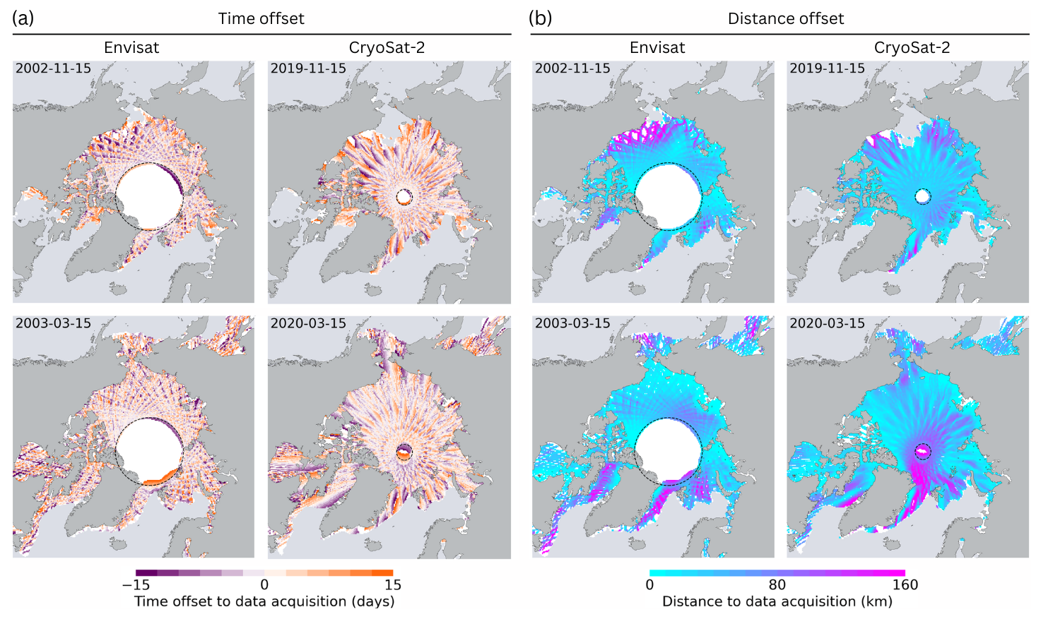
Figure 10 (a) Gridded time difference between the target day and the data acquisition time for Envisat (2002/2003) and CryoSat-2 (2019/2020) for 15 November and 15 March. (b) Same as (a) but for the geodesic distance between the parcel position on the target day and at the time of data acquisition. The white area in the background indicates data gaps with respect to the actual ice extent. The dashed circle represents the pole hole of the Envisat/CryoSat-2 orbit coverage.

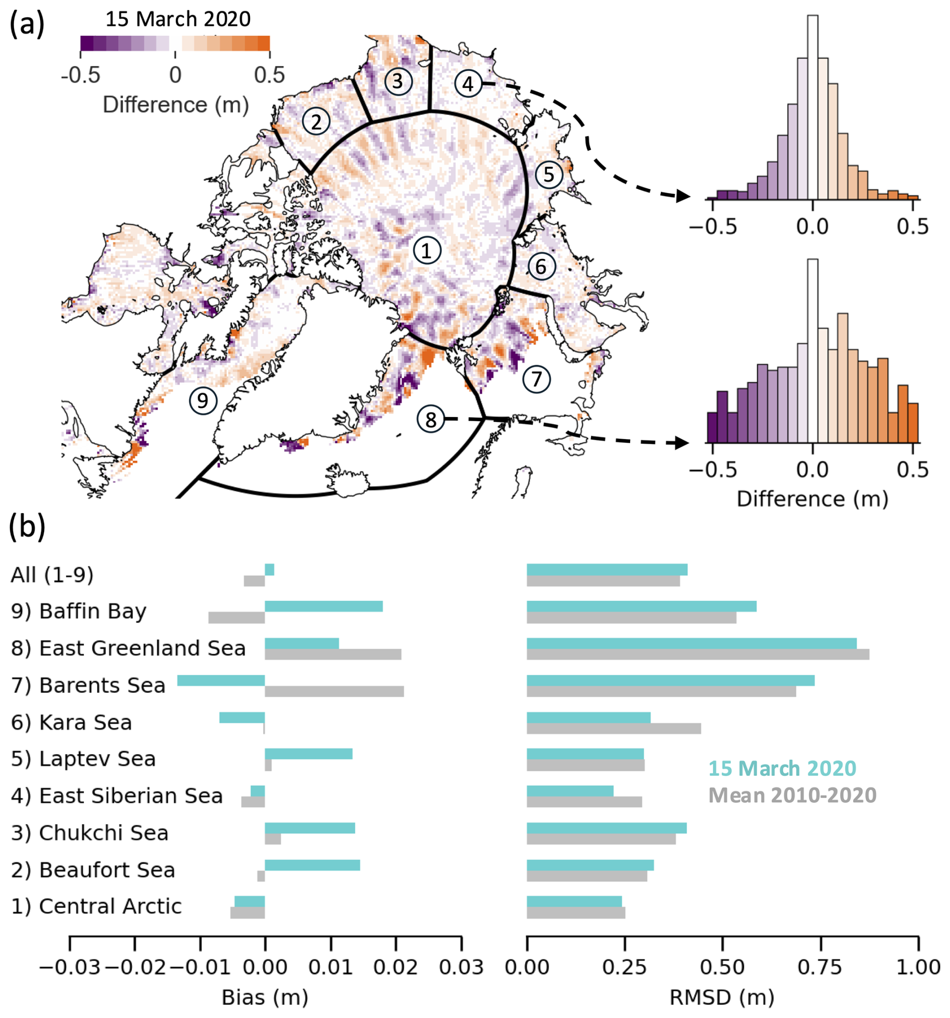
Figure 11 Intercomparison of DA-SIT and conventionally gridded SIT (C-SIT). (a) Difference map for 15 March 2020, including histograms of differences for the East Siberian Sea and East Greenland Sea. (b) Bias and root-mean-square deviation (RMSD) for marine regions on 15 March 2020, as well as the mean values over the 2010–2020 period.

4 Impact analysis

4.1 Time and distance offset to data acquisition

For each parcel, we track the time offset between the start and end of each parcel trajectory. The maximum offset is given by the time widow that defines over how many days along-track data are drift-corrected and stacked. In this study, we use ±15 d to be in line with the satellite subcycle. Figure 10a shows the gridded time offsets for the Envisat and CryoSat-2 DA-SIT parcels, considering the beginning (November) and end (April) of the winter season. Due to the drifting satellite orbit, we observe a track pattern with alternating time offsets in the meridional direction. The thickness change along the parcel trajectory correlates with the time offset because of thermodynamic ice growth, as well as the accumulation of deformation. As a consequence, when neglecting ice drift and ice growth corrections, the time offset pattern will cause track patterns in the monthly SIT maps.

Similarly, we calculate the geodesic distance between the final parcel position after drift correction and the position at the time of the measurements. Figure 10b shows the gridded geodesic distance for the same sensors and months as in Fig. 10a. The distance depends mainly on three factors. First, the travel distance scales with the temporal offset (Fig. 10a) for a given sea ice motion vector. Second, the magnitude of the sea ice drift and, third, its heading affect how far the parcel has traveled from the location of the satellite overflight. For example, high, south-moving ice drift in the Fram Strait leads to large distances to the location of data acquisition, scaled by the time offset. Those patterns are highly variable, as they directly depend on the sea ice drift. In the Fram Strait in March 2020, we find distances of up to 200 km, which is equal to the width of eight grid cells. This means that neglecting the ice drift correction in regions of high drift rates will cause the incorrect localization of thickness anomalies in heterogeneous sea ice regimes.

4.2 Comparison with conventional sea ice thickness grids

The key difference between the DA-SIT product and the baseline CCI SIT is the drift awareness, as DA-SIT is based on the same along-track retrievals. Therefore, we compare DA-SIT with the conventionally gridded C-SIT (Sect. 3.2). Here we only present the results from the CryoSat-2 era, as we find very similar results for the Envisat era. Figure 11a shows the difference map between DA-SIT and C-SIT for 15 March 2020. We divide the Arctic into the maritime regions introduced by Meier and Stewart (2023). For these regions, we calculate the bias and RMSD between DA-SIT and C-SIT, shown in Fig. 11b. The example from 15 March 2020 highlights regional differences in the magnitude of the impact of drift awareness. In the East Greenland Sea, including Fram Strait, we generally find the highest RMSD, while the lowest RMSD for March 2020 is found in the East Siberian Sea. Considering the entire CryoSat-2 era (2010–2020), the Arctic Ocean exhibits the lowest RMSD. As displayed by the histograms of differences in Fig. 11a, the distributions can be close to Gaussian or Laplacian in shape (e.g., East Siberian Sea) but can also be slightly skewed (e.g., East Greenland Sea). Typically, the smaller the area considered, the larger the differences. The pattern of differences in Fig. 11a reveals that the strongest impact of drift awareness is found in regions with strong sea ice drift, e.g., Fram Strait, Beaufort Gyre, and Barents Sea. In the Beaufort Sea region and north of it, we observe an alternating pattern of positive and negative differences in meridional direction. This originates from the fact that the C-SIT does not take into account the drifting along-track measurements, which contributes to the typical orbit track pattern (known as trackiness), which sometimes can be observed in the conventional SIT maps (Ricker et al., 2014). As expected, the DA-SIT product reduces this effect. The overall bias between DA-SIT and C-SIT is −0.33 cm for the period of 2010–2020 across all regions considered, which means that the impact on the mean Arctic SIT and volume time series is negligible.

5 Conclusions

We have presented a method to ensure drift awareness (DA) for sea ice thickness (SIT) maps derived from satellite altimetry and demonstrated its application on Envisat and CryoSat-2 data within the framework of the ESA Climate Change Initiative. The study included method descriptions, validation, and impact analysis. By applying DA, SIT retrievals from 1 month of altimetry measurements are projected onto 1 d, allowing us to produce daily maps of pan-Arctic SIT. This approach facilitates comparisons with SIT derived from passive microwave radiometer measurements (Tian-Kunze et al., 2014) or from in situ observations. From our findings in this study, we draw the following conclusions.

1. Validation with observational data. The DA-SIT method can capture anomalies observed in daily upward-looking sonar (ULS) averages, depending on the spatial extent of the anomalies and accurate colocation of measurements. This highlights the method’s capacity for improved regional analyses, although uncertainties in drift corrections must be considered.

2. Improvement in spatial representation. Drift awareness improves the spatial representation of sea ice thickness in gridded products by reducing regional biases (10–20 cm) and minimizing the displacement errors (up to 200 km) caused by neglecting sea ice drift. This improvement is particularly important in regions with strong drift, such as the Beaufort Sea and East Greenland Sea.

3. Regional vs. pan-Arctic effects. While regional-scale biases can be significant, the pan-Arctic mean differences between drift-aware SIT (DA-SIT) and conventional SIT maps are negligible (0.29 cm across all regions from 2010 to 2020; Fig. 11). This is because regional biases balance out on a longer scale, as ice is redistributed rather than lost.

4. Applications across missions. The DA algorithm is applicable to other satellite altimeters such as ERS-1/2, Sentinel-3A/B, and ICESat-2. Drift awareness should be integrated into future SIT mapping efforts to reduce uncertainties, especially when merging data from different missions, for example, radar (e.g., CryoSat-2) and laser altimeters (e.g., ICESat-2) to derive snow depth.

5. Future satellite missions. Drift awareness will be particularly important for new advanced altimeters, such as the Copernicus Polar Ice and Snow Topography Altimeter (CRISTAL) (Kern et al., 2020). To fully leverage the high-resolution measurements these systems provide, DA should be combined with higher-resolution drift products, e.g., derived from synthetic aperture radar (SAR) data (Howell et al., 2022) or future radiometer observations like the Copernicus Imaging Microwave Radiometer (CIMR) (Lavergne et al., 2021).

Overall, incorporating drift awareness into sea ice thickness mapping enhances the accuracy of gridded products, supports climate monitoring, and improves the understanding of sea ice dynamics. In the future, we plan to apply the drift awareness to altimetry retrievals in the Southern Ocean. Moreover, implementation of a column model that estimates dynamic and thermodynamic SIT growth along the DA trajectories could provide complementary information, which help to interpret the satellite-derived SIT estimates. Moreover, implementing near-real-time (NRT) processing using the most recent 15 d of altimetry data combined with NRT sea ice drift, has the potential to improve NRT SIT distributions.

Appendix A: Validation dataset overview

A1 AEM datasets

Table A1 lists the AEM data records for the period of 2007–2019, which are used for validation in this study, as well as the regions surveyed and the platform used.

Table A1 AEM data record overview used in this study. Data are only considered if they match the respective satellite product coverage.

A2 ULS datasets

Table A2 provides the position of the moorings in the Beaufort Sea and information about the ULS data record periods. They cover the Envisat (A, B, C, D) and the CryoSat-2 eras (A, B, D).

Table A2 Mooring sites with the ULS measurement periods used in this study.