Simulating the Holocene evolution of Ryder Glacier, North Greenland

The Greenland Ice Sheet's negative mass balance is driven by a sensitivity to a warming atmosphere and ocean. The fidelity of ice-sheet models in accounting for ice–ocean interaction is inherently uncertain and often constrained against recent fluctuations in the ice-sheet margin from the previous decades. The geological record can be used to contextualise ice-sheet mass loss and understand the drivers of changes at the marine margin across climatic shifts and previous extended warm periods, aiding our understanding of future ice-sheet behaviour. Here, we use the Ice-sheet and Sea-level System Model (ISSM) to explore the Holocene evolution of Ryder Glacier draining into Sherard Osborn Fjord, North Greenland. Our modelling results are constrained with terrestrial reconstructions of the paleo-ice-sheet margin and an extensive marine sediment record from Sherard Osborn Fjord that details ice dynamics over the past 12.5 ka years. By employing a consistent mesh resolution of <1 km at the ice–ocean boundary, we assess the importance of atmospheric and oceanic changes to Ryder Glacier's Holocene behaviour. Our simulations show that the initial retreat of the ice margin after the Younger Dryas cold period was driven by a warming climate and the resulting fluctuations in surface mass balance. Changing atmospheric conditions remain the first-order control in the timing of ice retreat during the Holocene. We find ice–ocean interactions become increasingly fundamental to Ryder's retreat in the mid-Holocene, with higher-than-contemporary melt rates required to force grounding line retreat and capture the collapse of the ice tongue during the Holocene Thermal Maximum. Regrowth of the tongue during the neoglacial cooling of the late Holocene is necessary to advance the terrestrial and marine margins of the glacier. Our results stress the importance of accurately resolving the ice–ocean interface in modelling efforts over centennial and millennial timescales, in particular the role of floating ice tongues and submarine melt, and provide vital analogies for the future evolution of Ryder in a warming climate.

1 Introduction

The rate of mass loss from the Greenland Ice Sheet (GrIS) has increased 5-fold between 1992 and 2020, culminating in a contribution to global mean sea level rise of 13.59±1.27 mm, roughly double that of the Antarctic Ice Sheet over the same period (Otosaka et al., 2023). Mass loss from Greenland can be partitioned between changes in the ice sheet's surface mass balance (SMB) (Box, 2013; Fettweis et al., 2020) and fluctuations at the marine interface of tidewater glaciers that drain the ice sheet's interior, known as discharge (Enderlin et al., 2014; Mouginot et al., 2019). Rising atmospheric temperatures have been the key driver of increased ablation and runoff from the ice sheet (Box et al., 2022), while the present influence of warm Atlantic Waters (AW) has been another major driver in the retreat and acceleration of Greenland's marine outlet glaciers (Slater and Straneo, 2022). However, there is a large spatial and temporal heterogeneity in the amplitude at which both processes affect mass loss across the ice sheet (Mouginot et al., 2019). As a consequence, projections of future sea level rise contribution from Greenland vary by an order of magnitude for high-emission scenarios (Goelzer et al., 2020). The largest uncertainties in such predictions stem from the limited ability of ice-sheet models to accurately resolve fluctuations in ice discharge from tidewater glaciers, where calving processes dominate mass loss and are estimated to account for up to 70 % of the ice sheet's sea level contribution by the end of the century (Goelzer et al., 2020; Choi et al., 2021). The fidelity of ice-sheet models in capturing such ice–ocean processes is often tested, and refined, against the satellite observation record. This implies that tidewater glacier behaviour can only be constrained across the most recent decades, when climatic conditions were distinctly cooler than what we expect in the future. Moreover, the ocean exhibits considerable natural variability on yearly to multi-decadal timescales. This complicates and potentially skews our interpretation of how oceanic changes affect the ice sheet (Khazendar et al., 2019). The geological record, however, can extend this history over centennial and millennial timescales to time periods similar to that of future projections. This provides valuable context for the observed ice-sheet behaviour over recent decades and important natural baselines and constraints for models of current and future ice-sheet change.

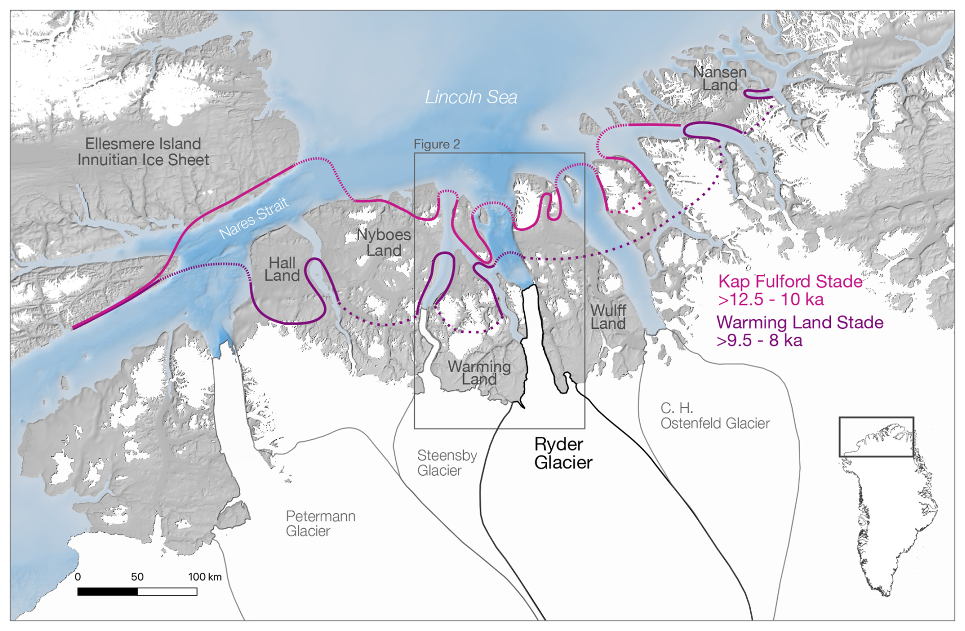
Figure 1 A map of northern Greenland highlighting the contemporary drainage basins of Petermann, Steensby, Ryder and Ostenfeld glaciers (Mouginot and Rignot, 2019). Paleo-ice-sheet margins of the Kap Fulford (>12.5–10 ka BP, pink) and Kap Warming Stade (>9.5–8 ka BP, purple) are shown as described in the terrestrial study by Kelly and Bennike (1992). Small dashed lines indicate hypothesised marine margins of GrIS, while large dashes are used to join data gaps.

The Holocene interglacial period presents the opportunity to study Greenlandic glacier behaviour across three distinct phases: first, the recession of the GrIS during the deglaciation following the Last Glacial Maximum (LGM) in response to rapidly warming temperatures (11.7–8.2 ka BP); second, the response of the ice sheet to the Holocene Thermal Maximum (HTM, 8.2–4.2 ka BP), a protracted period when Arctic temperatures were 3±1 °C above pre-industrial averages (Briner et al., 2016; Kaufman and Broadman, 2023); and third, the neoglacial cooling that began as early as 6.5–6.3 ka BP (Davis et al., 2009) and led into the Little Ice Age (LIA), where margins of the GrIS readvanced from a Holocene minimum towards a pre-industrial state (Kjær et al., 2022). Terrestrial studies have presented a detailed geological record of the GrIS margin evolution across different regions (e.g. Kelly and Bennike, 1992; England, 1999; Funder et al., 2011; Larsen et al., 2019; Young et al., 2021), culminating in a Greenland-wide reconstruction of ice-margin retreat during the early Holocene by Leger et al. (2024) (PaleoGrIS). Furthermore, marine geophysical mapping and marine sediment cores have provided additional knowledge of the timing of outlet glacier retreat and changing ice dynamics throughout the Holocene (Wangner et al., 2018; Reilly et al., 2019; Jakobsson et al., 2018; O'Regan et al., 2021). This is especially timely as paleo-ice-sheet modelling efforts are using increasingly fine resolution (<3 km) in regional studies in order to accurately resolve fjord-scale glacier dynamics and to assess the influence of ice–ocean interactions on the GrIS throughout the Holocene (Briner et al., 2020; Kajanto et al., 2020; Cuzzone et al., 2022).

Recognising the patterns and drivers of retreat during the Holocene, the current interglacial period, is especially pertinent to the northern sector of the GrIS. At the LGM, the ice sheet coalesced with the Innuitian Ice Sheet (England et al., 2006) and likely extended out into the Lincoln Sea where ice streams emanating from the Nares Strait and the northern fjords likely formed ice shelf conditions (Dawes, 1986; England, 1999; Larsen et al., 2010). During the Holocene, this marine-based ice system collapsed, as the GrIS decoupled from the Innuitian Ice Sheet and the northern outlet glaciers retreated back into their modern-day fjords. Owing to the remote nature of the region and harsh sea ice conditions, field surveys have been sparse and sporadic (Koch, 1928; Dawes, 1977; Weidick, 1978). Based on available data in the early 1990s, North Greenland's Holocene history was summarised into a series of Stades (Danish for stages) by Kelly and Bennike (1992) (Fig. 1). The Kap Fulford Stade relates to the most recent ice-sheet maximum, the Late Weichselian Glaciation, when the northern glaciers extended to the outer fjords and the GrIS and Innuitian ice sheets remained coalesced in Nares Strait. The retreat from this last maximum ice-sheet extent is proposed to have occurred >10.5 cal ka BP by O'Regan et al. (2021), after combining new marine radiocarbon dates and existing terrestrial dates (Kelly and Bennike, 1992). The Warming Land Stade follows between >9.5 and 8 cal ka BP, corresponding to a well-developed moraine sequence that represents a standstill of glacial retreat 20–60 km inland of the Kap Fulford Stade. Finally, the Steensby Stade characterises the neoglacial readvance of the GrIS from its Holocene minimum towards its most recent maximum in the LIA. While the onset of this readvance is poorly dated, it may have occurred prior to the late Holocene, perhaps as early as around 5.8 ka BP (O'Regan et al., 2021).

At present, northern Greenland contains enough ice to raise global mean sea levels by ∼93 cm (Mouginot et al., 2019). However, mass loss had been relatively subdued from the region until the 2000s, likely due to the buttressing of inland ice provided by floating ice tongues limiting ice discharge (Hill et al., 2017; Millan et al., 2018, 2023). Since 1978, the region's ice tongues have lost ∼25 % of their volume, with the notable collapse of Ostenfeld Glacier's ice tongue in 2003. Petermann, Steensby and Ryder glaciers remain buttressed by their floating ice tongues, yet they have all seen grounding line retreat and an acceleration of ice discharge explicitly linked to increasing basal melt rates beneath the floating ice (Hill et al., 2018a; Millan et al., 2023). During the Holocene, the ice tongues of Petermann and Ryder Glacier are believed to have disintegrated and retreated inland of the current grounding line positions (Jakobsson et al., 2018; Reilly et al., 2019; O'Regan et al., 2021). Such behaviour could serve as a potential analogy for the future evolution of the contemporary outlet glaciers, where the collapse of their floating ice tongues may accelerate ice discharge and the region's contribution to global sea level rise (Hill et al., 2018b; Humbert et al., 2023).

Here we use the Ice-sheet and Sea-level System Model (ISSM; Larour et al., 2012) to explore the dynamics of Ryder Glacier during the Holocene, constrained by unique marine sediment archives, mapped submarine glacier landforms and terrestrial evidence. Focusing on a single outlet glacier allows us to employ a model that resolves ice–ocean and grounding line dynamics in high resolution (<1 km). This puts more confidence in our simulations and gives us the opportunity to provide a new, more detailed understanding of how Ryder Glacier and its ice tongue responded to a warming atmosphere and ocean.

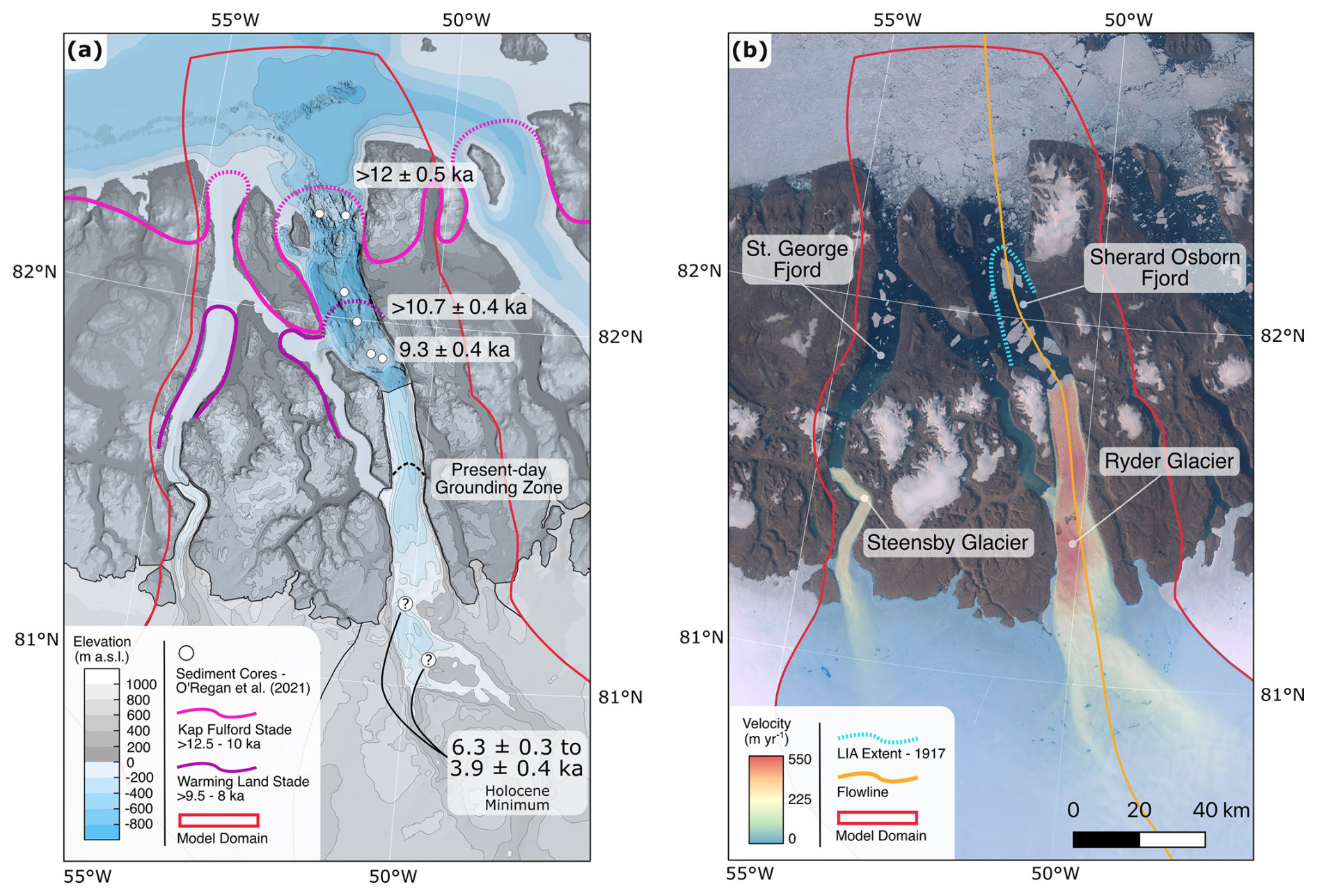
Figure 2 (a) A topographic map of Ryder and Steensby Glacier. Both the bathymetry and topography are taken from BedMachine v5 (Morlighem et al., 2022). Paleo-ice-sheet margins of the Kap Fulford Stade (>12.5–10 ka BP, pink) and Warming Stade (>9.5–8 ka BP, purple) are redrawn from Kelly and Bennike (1992). Sediment cores taken during the Ryder expedition on icebreaker Oden are shown by white circles and are accompanied by minimum ages (O'Regan et al., 2021). (b) A satellite image of Ryder and Steensby glacier draining into Sherard Osborn and Saint George Fjord from summer 2019 (MacGregor et al., 2020). Ice velocities are taken from MEaSUREs (Joughin et al., 2016, 2018). A centre flowline for Ryder Glacier is shown in orange, the Little Ice Age extent of the glacier is highlighted in dashed blue (Koch, 1928) and the model domain used in the study is shown in red.

2 Ryder Glacier

Ryder Glacier currently drains the GrIS into Sherard Osborn Fjord (Fig. 2), where a floating tongue extends ∼25–30 km from the grounding line and velocities peak at 500 m yr⁻¹ (Wilson et al., 2017; Hill et al., 2017). Sherard Osborn Fjord continues ∼70 km from the present-day grounding line toward the Lincoln Sea, reaching a maximum depth of 890 m and containing two shallow bathymetric sills, an outer (375–475 m below sea level) and inner sill (193–390 m below sea level), with the latter thought to play a key role in shielding the glacier from sub-surface warm Atlantic Waters (AW) (Jakobsson et al., 2020; Nilsson et al., 2023). The floating terminus has remained relatively stable since the 1990s, undergoing a cyclic pattern of slow advance followed by retreat, potentially controlled by fjord geometry (Holmes et al., 2021). This stability has persisted despite a retreat of the grounding line by ∼8 km since 1992 (Millan et al., 2023).

During the Ryder 2019 expedition with the Swedish icebreaker Oden, numerous sediment cores were taken in Sherard Osborn and have been used to describe the Holocene behaviour of Ryder Glacier by O'Regan et al. (2021) (Fig. 2a). Radiocarbon dating and analysis of six lithologic units (LU) detail an evolution of the glacier that generally aligns with the terrestrial record of retreat described in Kelly and Bennike (1992). The first two lithologic units (LU6 and LU5) comprise a transition from glaciomarine diamicton to a laminated meltwater-dominated facies as the grounding line of Ryder Glacier began to retreat from the fjords' outer sill. Ages of 12 ± 0.5 ka BP (LU6) on the outer sill and 10.7±0.4 ka BP (LU5) in the mid-fjord region align with the Kap Fulford Stade, while the beginning of sedimentation on the inner sill at 9.3±0.4 ka BP (LU5) corresponds to the Warming Land Stade. A further laminated sub-ice-shelf facies follows (LU4: 7.6±0.4 to 6.3±0.3 ka BP) before a second diamict facies spanning 6.3±0.3 to 3.9±0.4 ka BP (LU3) occurs and hints at the collapse of the ice tongue during the HTM. The low sedimentation rates during this period are suggested to mark the retreat of Ryder Glacier into a small isolated embayment, ∼40 km upstream of the present-day grounding line (Fig. 2a). Such retreat would have reduced the delivery of fine-grained meltwater-entrained sediments but still allowed for icebergs to deposit ice-rafted debris (IRD) in the fjord. The following lithologic facies after 3.9±0.4 ka BP (LU2 and LU1), in line with the Steensby Stade described by Kelly and Bennike (1992), show a transition from open-water bioturbated sediments to laminated facies that indicate the regrowth and advance of Ryder's ice tongue towards the outer sill. Lauge Koch mapped Ryder's LIA extent in 1917 during the Second Thule Expedition, showing the ice tongue had extended toward the mouth of Sherard Osborn Fjord and the outer sill (Fig. 2b).

3 Methods

The finite-element thermomechanical ice-sheet model ISSM is employed to simulate the Holocene history of Ryder Glacier (Larour et al., 2012) together with a higher-order (HO) approximation (Blatter, 1995; Pattyn, 2003) of the full Stokes (FS) equations. We use the HO approximation as it balances computational efficiency with thermomechanical 3D ice dynamics, including higher-order stresses and temperature-dependent viscosity, which are critical when simulating ice evolution over paleo-timescales. Although we recognise that FS offers greater accuracy in regions such as the grounding line, where the inclusion of bridging stresses, neglected in the HO approximation, are important, it remains computationally infeasible to use over extended timescales such as the Holocene. To better capture grounding migration, we run our HO model at resolutions of <1 km, following a model set-up that is similar to Briner et al. (2020) and Cuzzone et al. (2022) that performed well when simulating terrestrial and marine regions of the GrIS over the Holocene.

3.1 Model domain and set-up

Our model domain is based on the present-day drainage catchment of Ryder Glacier, defined from velocity and slope angles of the ice surface (Mouginot and Rignot, 2019). The domain is then extended northward to include Sherard Osborn Fjord and ∼30 km north into the Lincoln Sea to capture the LGM extent of Ryder Glacier (Fig. 2b). On the eastern side of the domain we follow the topographic divide in Wulff Land, while also extending the domain westward to include the neighbouring Steensby Glacier and Saint George Fjord. We do this in order to capture any effects arising from the two glaciers merging towards the Lincoln Sea owing to the connected fjord systems. We define the base of our domain using bedrock topography from BedMachine v5 (Morlighem et al., 2022), which contains the high-resolution bathymetric data of Sherard Osborn Fjord surveyed by the Swedish icebreaker Oden in 2019 (Fig. 2a; Jakobsson et al., 2020). The initial ice surface for our model is also taken from BedMachine v5, before it evolves in our Younger Dryas spin-up (Sect. 3.5).

A non-uniform mesh of the domain is produced from modern ice velocities and bedrock topography (Joughin et al., 2016; Morlighem et al., 2022). Elements range from 10 km in size for the slow-moving ice in the upper regions of the domain, decreasing to 750 m where velocities exceed 400 m yr⁻¹ as well as in contemporary ice-free fjord areas. This ensures that grounding line migration is simulated at resolutions of <1 km for the entirety of our simulations – a resolution necessary for capturing such dynamics (Seroussi and Morlighem, 2018). The domain is then extruded vertically to contain five layers, and following Cuzzone et al. (2018) we use cubic finite elements along the z axis (prisms P1 × P3) for vertical interpolation to capture sharp thermal gradients near the base of the ice sheet without additional, computationally expensive, layers.

We use an enthalpy formulation from Aschwanden et al. (2012) to simulate ice temperature throughout our simulations, applying a constant geothermal heat flux at the base (Shapiro and Ritzwoller, 2004) and transient air temperatures at the surface (Sect. 3.4). The ice rheology parameter B is initialised by solving for a present-day thermal state and allowed to vary transiently following the rate factors in Cuffey and Paterson (2010).

Basal friction is modelled through the linear viscous Budd law (Budd et al., 1979), defining basal drag (τ_b) as

$$\begin{array}{}\text{(1)}& {\mathit{\tau }}_{\mathrm{b}}=-k^{\mathrm{2}}N{v}_{\mathrm{b}},\end{array}$$

where k is a friction coefficient, N is effective pressure and v_b is the basal velocity. The friction coefficient, k, for present-day ice areas is inverted for using an adjoint method (Morlighem et al., 2010, 2013) that fits with modern velocities (Joughin et al., 2016, 2018). For contemporary non-ice areas we define a friction coefficient as a function of elevation similar to Åkesson et al. (2018a):

$$\begin{array}{}\text{(2)}& k=\mathrm{100}\times {\displaystyle \frac{\text{min}\left(\text{max}(\mathrm{0},z_{\mathrm{b}}+|\text{min}\left(z_{\mathrm{b}}\right)|,\text{max}(z_{\mathrm{b}})\right)}{\text{max}\left(z_{\mathrm{b}}\right)}}\end{array}$$

where z_b is the bedrock elevation relative to sea level (Morlighem et al., 2022). This produces a low friction coefficient in the deep fjords, where we would expect fast-flowing ice, and larger values across topographic highs, where ice is expected to flow slower. This spatial distribution of friction coefficients is kept fixed over time. Meanwhile, we follow Cuzzone et al. (2019) to allow the friction field to be scaled transiently based on changes in the simulated evolution of basal temperatures relative to basal temperatures from a present-day thermal steady state of the glacier. This implementation produces an increase in friction for colder temperatures during the YD, while also rendering more slippery conditions during warmer periods such as the HTM.

We apply Dirichlet boundary conditions of ice thickness, velocity and temperature on the eastern and western boundaries of our domain. These boundary conditions are taken from a continental-scale model of GrIS simulated across the same timescales with a similar model set-up, albeit at a coarser resolution (Briner et al., 2020). We use different boundary conditions for each of our SMB scenarios (Sect. 3.4), aligning with the experiments found in Briner et al. (2020). We justify the use of these boundary conditions as running a continental-scale simulation at an equivalent resolution would be computationally infeasible. Furthermore, by using consistent boundary conditions across our model runs, we isolate the effects of our applied climate forcings on glacier behaviour. Finally, ice is allowed to freely leave the domain at the northern boundary.

All model simulations are run for 12 550 years from 12 500 BP, where P is defined as 1950 CE to 2000 CE, using an adaptive time step that varies between 0.02 and 0.3 years while satisfying the Courant–Friedrichs–Lewy criterion (Courant et al., 1928).

3.2 Calving parameterisation and ice-front migration

Ice-front migration is handled within ISSM using the level-set method (Bondzio et al., 2016). The ice-front boundary moves at velocity

$$\begin{array}{}\text{(3)}& {\mathit{v}}_f=\mathit{v}-(c+M)\mathit{n},\end{array}$$

where v is the velocity vector at the ice front, c and M are the calving and melting rate, respectively, and n is the normal vector pointing outward, orthogonal to the level set defined as a signed-distance field. During our simulations we assume that horizontal melt at the front of an ice tongue is negligible compared to calving and ocean-induced melt from below. Thus, we focus on applying melt rates to beneath ice that has reached flotation (Sect. 3.3).

A von Mises law is used to parameterise calving (Morlighem et al., 2016), where the calving rate, c, depends on the von Mises tensile stress, $\stackrel{\sim }{\mathit{\sigma }}$, and a predefined maximum stress threshold value, σ_max (Table 1):

$$\begin{array}{}\text{(4)}& c=\left|\mathit{v}\right|{\displaystyle \frac{\stackrel{\sim }{\mathit{\sigma }}}{\mathit{\sigma }{}_{\text{max}}}}.\end{array}$$

As such, calving can only occur when $\stackrel{\sim }{\mathit{\sigma }}>\mathit{\sigma }{}_{\text{max}}$; when $\stackrel{\sim }{\mathit{\sigma }}<\mathit{\sigma }{}_{\text{max}}$ then c=0. This calving parameterisation has been successfully used to simulate the migration of grounded and floating Greenlandic ice fronts in both modern (Morlighem et al., 2016; Choi et al., 2018; Åkesson et al., 2022) and paleo settings (Kajanto et al., 2020; Cuzzone et al., 2022).

3.3 Ocean melt

An ocean melt rate is applied to floating ice as a linear function of depth. Melt rate increases from 0 m yr⁻¹ at depths shallower than 100 m to a predefined deepmelt value at depths below 400 m (Table 1). This implementation matches the distribution of submarine melt found through both observations and ocean modelling of Ryder Glacier (Wilson et al., 2017; Wiskandt et al., 2023), capturing the highest melt rates towards the grounding line, driven by the interplay with subglacial discharges and warmer ocean waters, before decreasing in the cooler polar surface waters found in the upper 100 m of the fjord. Horizontal melt at the front of the ice tongue is assumed negligible, in line with melt at depths shallower than 100 m and under the premise that frontal ablation is dominated by calving processes while submarine melt primarily acts near the grounding line beneath ice tongues (Wilson et al., 2017; Holmes et al., 2021). In the event of an ice tongue collapse, melt is applied uniformly to the submerged grounded glacier front at half the defined deepmelt value in order to account for a decrease in melt towards the water line.

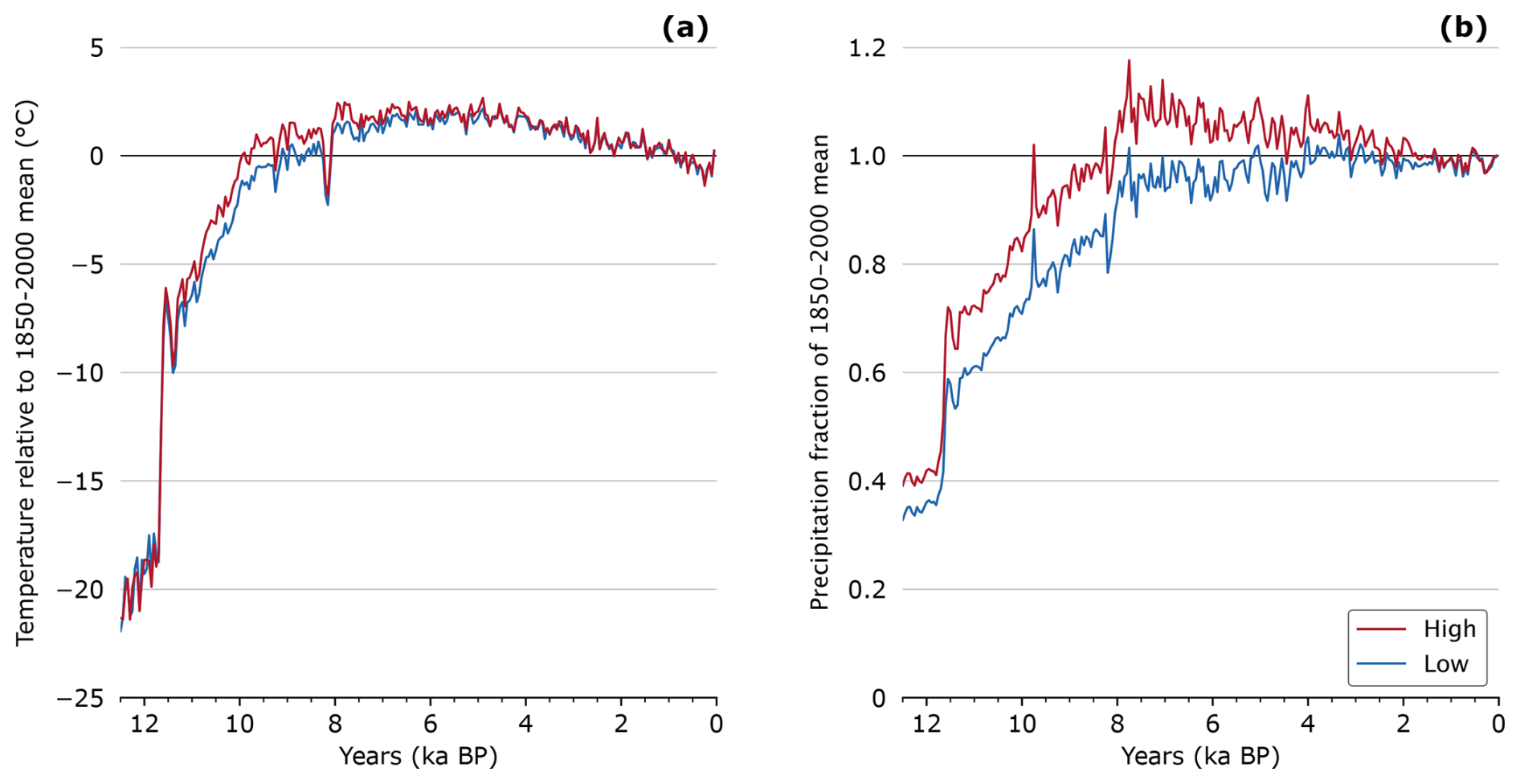
Figure 3 Mean annual climate data during the Holocene averaged over the model domain taken from Badgeley et al. (2020). (a) High (red) and low (blue) Holocene temperature scenarios expressed as anomalies with respect to a 1850 to 2000 mean (Box, 2013). (b) High (red) and low (blue) Holocene precipitation scenarios expressed as fractions of a 1850 to 2000 mean (Box, 2013).

3.4 Holocene climate

Holocene SMB is computed using a positive degree day (PDD) model (Tarasov and Peltier, 1999), forced with paleoclimate reanalysis data from Badgeley et al. (2020). The model assumes that snow melts at 3 mm °C⁻¹ d⁻¹ followed by ice melt at 8 mm °C⁻¹ d⁻¹ for the remaining positive degree days (Braithwaite, 1995; Born and Nisancioglu, 2012; Plach et al., 2018). The formation of superimposed ice is allowed following Janssens and Huybrechts (2000). Finally, a lapse rate of 6 °C km⁻¹ is used to adjust the climate forcings to transient changes in the glacier's elevation.

Temperature and precipitation for the PDD model is taken from a paleoclimate reanalysis dataset produced by Badgeley et al. (2020) through the assimilation of climate model simulations and proxy data. The TraCE21Ka climate model output (Liu et al., 2009; He et al., 2013) is used in conjunction with oxygen-isotope records from eight ice cores and ice layer thicknesses from five ice cores to reconstruct temperature and precipitation, respectively. The resulting dataset contains a number of different temperature and precipitation pathways, varying spatially at a 50-year temporal resolution, covering the Holocene.

We follow Cuzzone et al. (2022) in using four different Holocene SMB forcings produced from combinations of the high and low reconstructions of temperature and precipitation (Fig. 3a and b). These reconstructed variables represent the upper and lower bands of scenarios discussed in Badgeley et al. (2020) and provide a cost-effective way of testing the impact of both climate drivers during the Holocene. We hereby refer to each SMB scenario using the following notation: temperature/precipitation, where, for example, High/Low would describe the SMB scenario produced from the high-temperature and low-precipitation pathways.

The aforementioned paleoclimate variables, temperature and precipitation, are expressed as anomalies from an 1850–2000 mean and a fraction of an 1850–2000 mean, respectively. We therefore use the comparable monthly climate variables from Box (2013) to produce the final temperature and precipitation variables need for the PDD model:

$$\begin{array}{}\text{(5)}& {\displaystyle }{T}_t={\stackrel{\mathrm{‾}}{T}}_{\mathrm{1850}-\mathrm{2000}}+\mathrm{\Delta }{T}_t,\text{(6)}& {\displaystyle }{P}_t={\stackrel{\mathrm{‾}}{P}}_{\mathrm{1850}-\mathrm{2000}}\times \mathrm{\Delta }{P}_t,\end{array}$$

where ${\stackrel{\mathrm{‾}}{T}}_{\mathrm{1850}-\mathrm{2000}}$ and ${\stackrel{\mathrm{‾}}{P}}_{\mathrm{1850}-\mathrm{2000}}$ are the monthly mean temperature and precipitation dates from Box (2013), and ΔT_t and ΔP_t are the corresponding paleo-anomalies from Badgeley et al. (2020). Every model run uses the Holocene climatology from 12 500 BP until 1850 CE, with the final 150 years using the mean modern values from Box (2013).

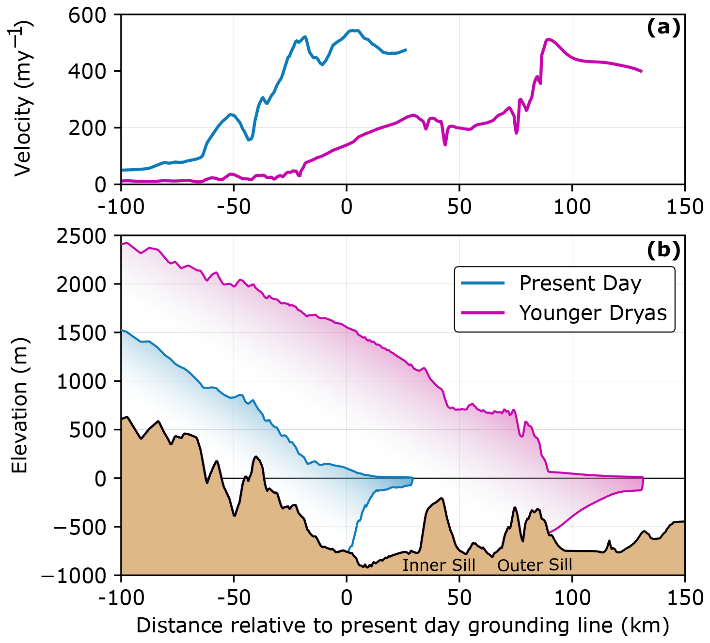
Figure 4 A comparison between the present-day Ryder Glacier (blue) and that of the glacier after running a 20 000 year spin-up forced with a YD climate from SMB scenario Low/High (pink). (a) The velocity profile along the glacier's centre flowline. (b) A 2D cross-section profile along the centre flowline. Bedrock data and the present-day ice surface is from BedMachine v5 (Morlighem et al., 2022). Spin-up geometry from all SMB scenarios can be found in Fig. S2 in the Supplement.

3.5 Younger Dryas spin-up

We perform a Younger Dryas (YD) model spin-up to obtain an initial ice-sheet state that is both geologically consistent and internally coherent. We assume that Ryder Glacier remained stable during the YD, consistent with the earliest recovered sediments from Sherard Osborn Fjord (12±0.5 ka BP), which indicate that the grounding line had not yet begun to retreat and was likely positioned on the outer sill (O'Regan et al., 2021). Although other sectors of the Greenland Ice Sheet (GrIS) began to retreat from their LGM extents prior to the YD, retreat in the northern sector was comparatively limited (Leger et al., 2024). In this region, the grounding lines of the major outlet glaciers remained stable at or near the fjord mouths, typically grounded on bathymetric highs, until the onset of early Holocene warming (Kelly and Bennike, 1992; England, 1999; Jennings et al., 2011; Jakobsson et al., 2018; Jennings et al., 2019; O'Regan et al., 2021).

We begin our spin-up simulations using an initial modern-day ice surface from BedMachine v5 (Morlighem et al., 2022) and force the model with a constant climate from 12 500 BP. We conduct a spin-up for the four different SMB scenarios, maintaining consistent boundary conditions of ice thickness, temperature and velocities from the larger continental-scale model (cf. Sect. 3.1). It takes 20 000 model years until ice volume, temperature and velocities reach an equilibrium. We do not allow calving during the spin-up. Ocean melt is applied after the first 2000 years, in order to allow for grounding line advance, after which the deepmelt rate is set to 10 m yr⁻¹. While an arbitrary choice, we argue that ocean melt at the YD would be substantially lower than contemporary rates at Ryder Glacier (Wilson et al., 2017), due to both colder ocean temperatures and a reduction in subglacial discharge in a climate with little surface melt (Fig. 3a). The combination of ocean melt and atmospheric forcings results in a spun-up Ryder Glacier that aligns with the geological record at the YD, with the grounding line resting atop the outer sill where the oldest sediments recovered from Sherard Osborn Fjord are dated to 12±0.5 ka BP (Fig. 4; O'Regan et al., 2021). Furthermore, the ice shelf emanating from the fjord also matches the hypothesised Lincoln Sea Ice Stream and ice shelf conditions across northern Greenland (Funder and Larsen, 1982; Dawes, 1986; Larsen et al., 2010). The final spun-up state across the four different SMB scenarios is very consistent (Fig. S2), owing to little climatic variation between the SMB scenarios at the YD (Fig. 3). These four YD states provide the initial conditions for our Holocene transient runs.

3.6 Transient experiments

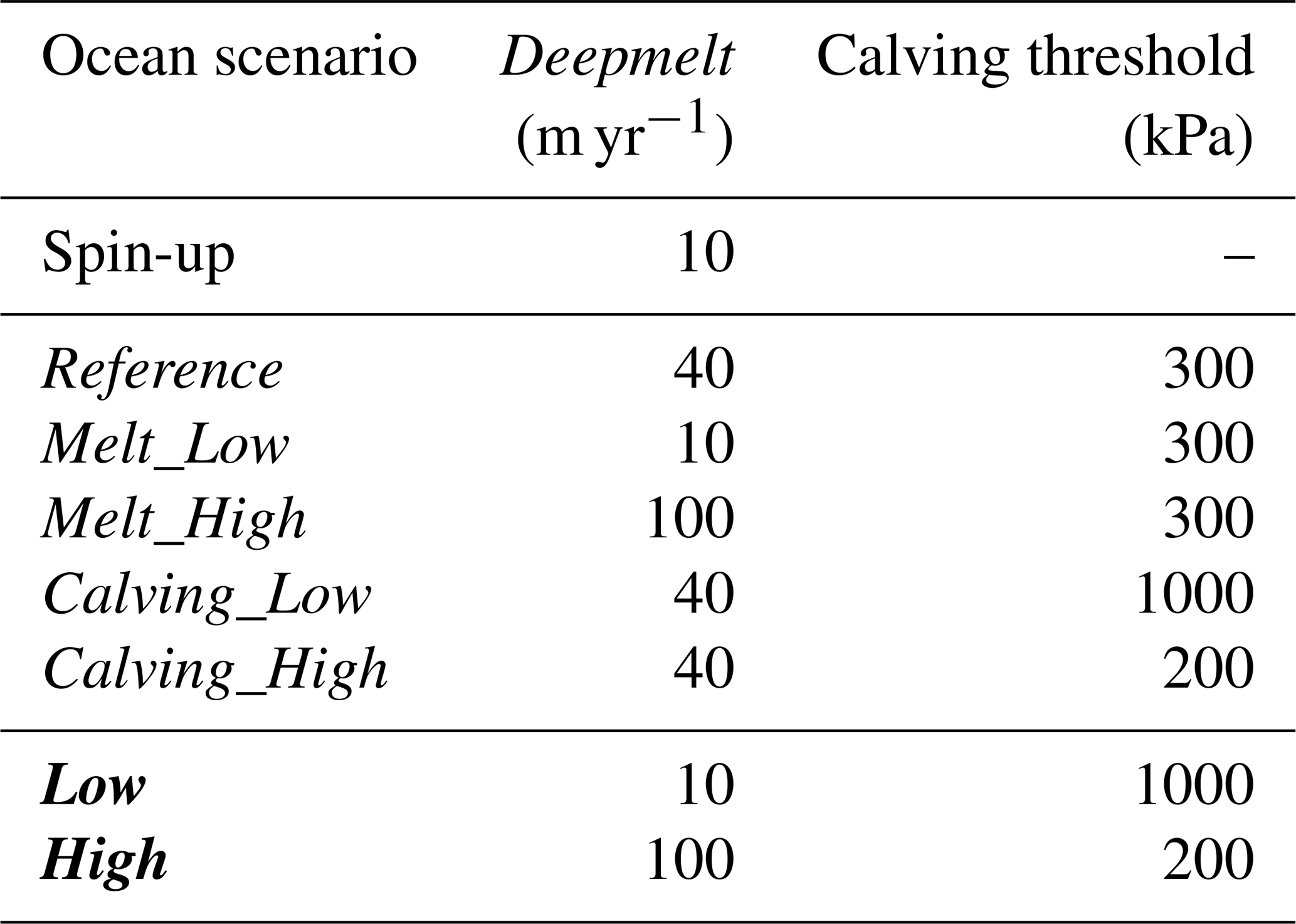
Our transient experiments are designed to assess how atmospheric and ocean–ice interactions influenced the retreat of Ryder Glacier in the Holocene. We begin with five initial oceanic scenarios that vary the calving threshold (Sect. 3.2) and ocean deepmelt rate (Sect. 3.3) from modern Reference values (Table 1). These five sets of ocean forcings are run across the four different Holocene SMB scenarios previously discussed (Sect. 3.4).

Our Reference calving threshold for floating ice is 300 kPa as this value was able to reproduce the recent evolution of Ryder Glacier's floating tongue (Fig. S1) and aligns with the threshold used in a study of the neighbouring Petermann glacier by Åkesson et al. (2022). Because calving laws are often calibrated for glaciers in specific states, influenced by factors such as fjord geometry, bedrock topography and ice rheology (Amaral et al., 2020; Wilner et al., 2023), we acknowledge that our chosen Reference calving threshold is unlikely to remain valid throughout the entire Holocene. To evaluate the influence of the calving threshold on ice dynamics, we conduct transient simulations with varied threshold values. For our High_Calving scenario, we lower the threshold to be 200 kPa to implicitly account for an extended calving period during the HTM when sea ice conditions were more seasonal (Detlef et al., 2023). Conversely, we set a threshold of 1000 kPa for our Low_Calving scenario, the same value as our grounded ice calving threshold, with the idea of preserving Ryder Glacier's floating tongue throughout the Holocene. At the beginning of all transient runs the floating calving threshold is set to 1000 kPa before linearly transitioning to the defined value in the ocean scenario between 11 500 and 10 000 ka BP as temperatures rise from the YD into the Holocene.

For melt under the floating tongue, we set our Reference value for deepmelt to be 40 m yr⁻¹. This aligns with oceanic modelling studies of Ryder Glacier, as well as satellite observations of Ryder and other northern Greenlandic glaciers (Wilson et al., 2017; Millan et al., 2023; Wiskandt et al., 2023). For a High_Melt scenario we set the deepmelt rate as 100 m yr⁻¹, similar to modelled peak melt rates under Ryder Glacier's ice shelf with a warming of AW temperatures by 2 °C (Wiskandt et al., 2023). For a Low_Melt scenario we take a deepmelt rate of 10 m yr⁻¹, the same value used in the YD model spin-up. The transition from a consistent deepmelt rate of 10 m yr⁻¹ during our spin-up simulations to the defined melt rate for the transient simulation occurs linearly between 11 500 and 10 000 BP.

Furthermore, we run two extreme ocean scenarios, here termed High and Low, where we combine the respective deepmelt rates and floating calving thresholds from their individual high and low scenarios together. These two ocean scenarios are only run with the upper and lower limits of our SMB pathways.

Table 1 A summary of different ocean forcings with respective calving thresholds for floating ice and submarine melt values. In bold are the ocean scenarios that are only run with the upper and lower SMB scenarios (Fig. 3): high temperature and low temperature (High/Low) as well as low temperature and high precipitation (Low/High). Note that the spin-up stimulations do not include calving.

4 Results

Here we describe the results of our Holocene transient simulations of Ryder Glacier by first focusing on the marine retreat and ice dynamics of the glacier (Sect. 4.1), followed by the terrestrial evolution of the ice-sheet margin (Sect. 4.2).

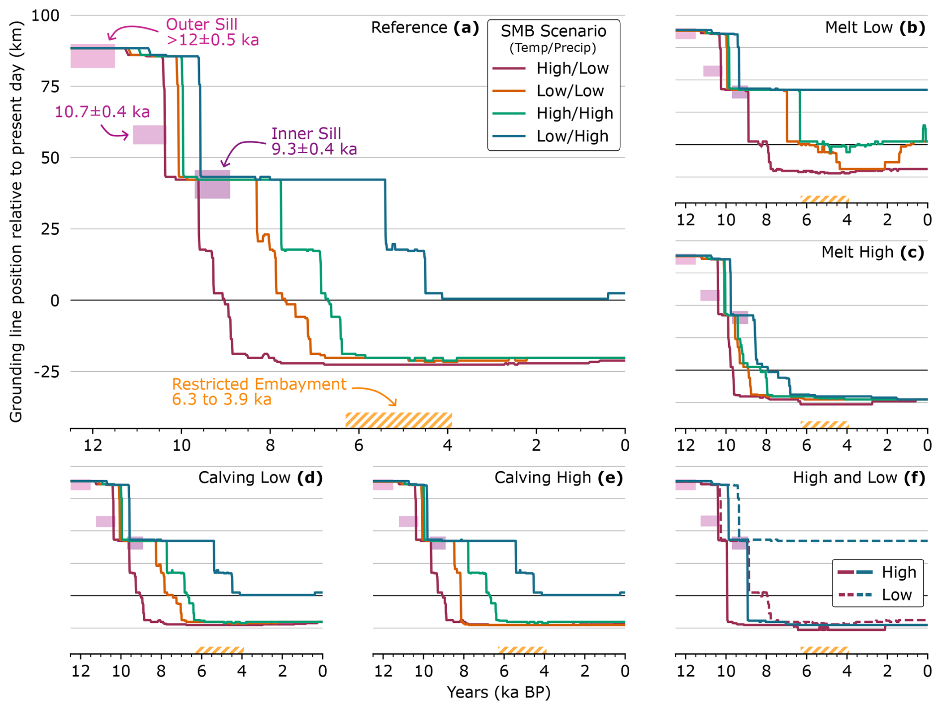
Figure 5 Evolution of the grounding line relative to Ryder's present-day position for all transient runs. Line colour defines the SMB scenario for the transient runs: High/Low (red), Low/Low (Orange), High/High (Green) and Low/High (Blue). Each subplot represents a different ocean scenario: (a) Reference, (b) Melt_Low, (c) Melt_High, (d) Calving_Low, (e) Calving_High, and (f) both the extreme High and Low ocean forcings. Shaded boxes highlight the position of sediment cores and their minimum ages, alongside possible timing of retreat into the restricted embayment upstream of the present-day grounding line. All dates are sourced from O'Regan et al. (2021).

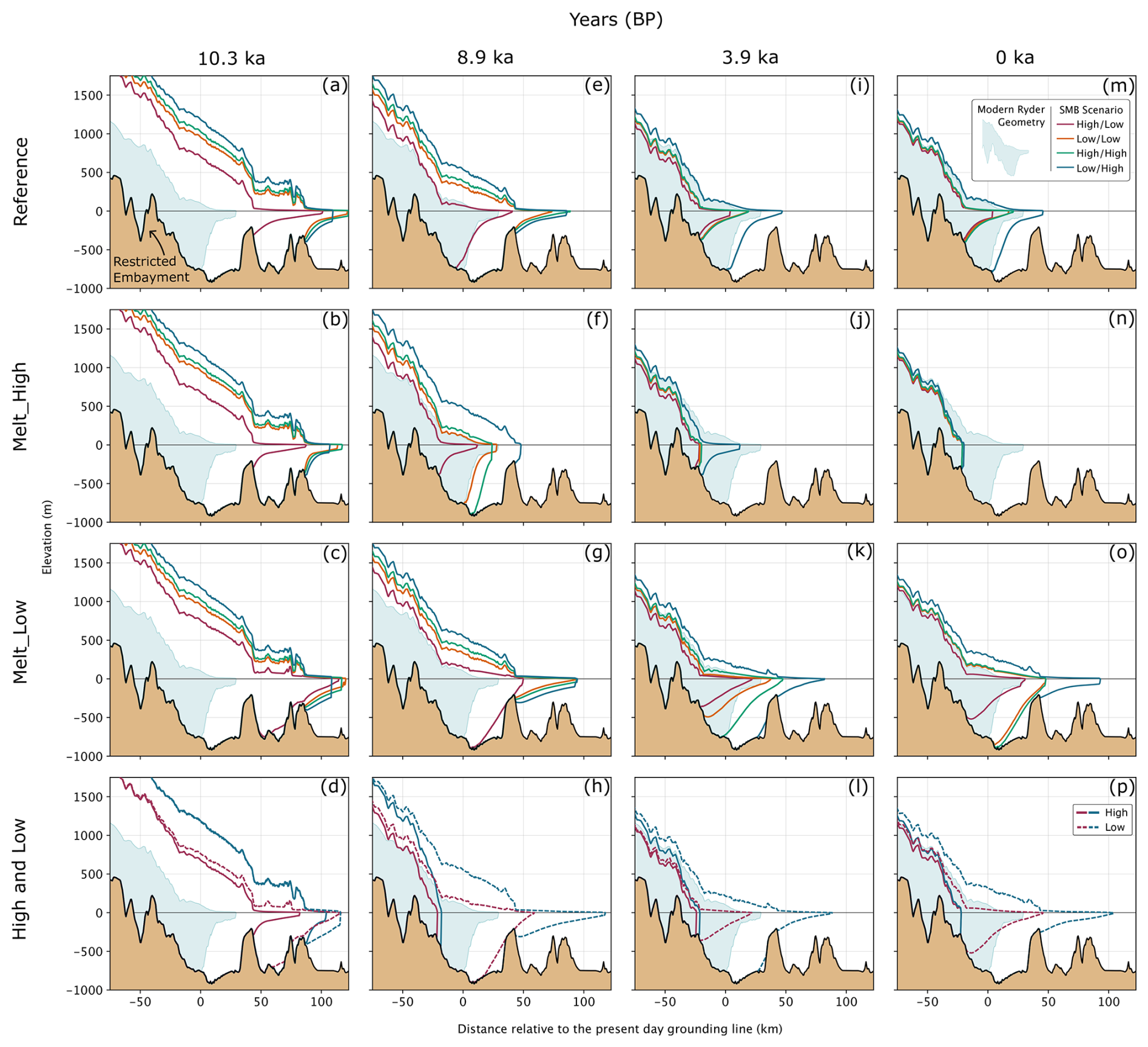
Figure 6 Evolution of Ryder Glacier in 2D cross-section views along the centre flowline during the Holocene at specific time stamps. Dates of 10.3 ka (a–d), 8.9 ka (e–h), 3.9 ka (i–l) and 0 ka (m–p), represent specific landmarks in the evolution of Ryder as discussed in O'Regan et al. (2021). Each row represents a different ocean forcing used in the transient simulation (Table 1), from top down this includes Reference, Melt_High, Melt_Low, and both extreme High and Low scenarios. Ocean scenarios Calving_High and Calving_Low are found in the Supplement as their behaviour does not differ considerably from the Reference scenario (Fig. S3). Each plot contains the four different SMB scenarios: High/Low (red), Low/Low (Orange), High/High (Green) and Low/High (Blue).

4.1 Marine Holocene evolution

The evolution of Ryder Glacier in our simulations is described in the context of the lithologic units (LU) taken from sediment cores taken in Sherard Osborn Fjord that can be used for an idealised comparison of the glacier's behaviour (O'Regan et al., 2021).

4.1.1 Early Holocene retreat

Ryder Glacier retreats from the outer sill between 10.4 and 9.4 ka BP in all of our Holocene simulations (Fig. 5). This is ∼2000 years later than indicated by the age of the oldest sediments recovered from the outer sill in Sherard Osborn Fjord, which are dated to 12±0.5 ka BP (LU6). The simulated retreat dates instead align well with the basal age of the next lithologic boundary, LU5, dated to 10.7±0.4 ka BP, found between both sills in Sherard Osborn Fjord, which marks the beginning of sedimentation in the mid-fjord region (Fig. 2a).

There is minimal variation in the timing of retreat from the outer sill across the different ocean scenarios (Fig. 5), with the glacier's geometry very consistent at 10.3 ka (the minimum age of LU5; Fig. 6a–d). Instead, retreat varies with the choice of SMB pathways, that is, for high or low scenarios of temperature and precipitation. Simulations using the High/Low (temperature/precipitation) scenario retreat first (10.4 to 10.2 ka BP), followed by Low/Low (10.2 to 9.9 ka BP) and High/High (10 to 9.8 ka BP) and finally Low/High (9.8 to 9.4 ka BP). We consistently observe that this sequence of SMB scenarios dictates the timing of retreat within each ocean forcing throughout the Holocene (Fig. 5).

While the timing of retreat from the outer sill differs between SMB scenarios, the pattern and pace of retreat does not. In all runs, once Ryder begins to detach from the outer sill the grounding line quickly retreats ∼40 km in less than 50 years (Fig. 5), implying a mean retreat rate >800 m yr⁻¹. Notably, there is no grounding line standstill in the deeper mid-fjord, and continuous retreat is observed, irrespective of the choice of atmospheric and oceanic forcing, until the grounding line reaches the inner sill. Here, the grounding line remains stable in all runs for at least 500 years. It is noted here that simulations Low/High (Melt_Low) and Low/High (Low) do not retreat further than the inner sill (Fig. 5b and f).

Our simulations show a wide range of dates for retreat from the inner bathymetric high: 9.7 to 5.4 ka BP (Fig. 5). For runs forced with ocean scenarios – Reference, Calving_Low and Calving_High – retreat ages are consistently between 9.6 and 5.4 ka BP (Fig. 5a, d and e). The timing of retreat for simulations using the Melt_Low ocean forcing is later, between 8.9 and 6.4 ka BP, albeit with Low/High (Melt_Low) remaining on the inner sill for the remainder of the Holocene simulation (Fig. 5b). Dates of retreat from the inner sill are earlier and much more concentrated for runs forced with Melt_High and High ocean scenarios, at 9.9 to 8.7 ka BP and 10 to 9 ka BP, respectively (Fig. 5c and f).

It is only in simulations using an elevated ocean melt in Melt_High and High ocean forcing, as well as all runs forced with the most extreme SMB of high temperature and low precipitation (High/Low), that we see both grounding line retreat and the floating tongue detached from the inner sill that matches the onset of continuous sedimentation at this location: 9.3±0.4 ka BP (LU5; Fig. 6e–h). All remaining simulations remain grounded on the inner sill until at least ∼8.3 ka BP (Fig. 5).

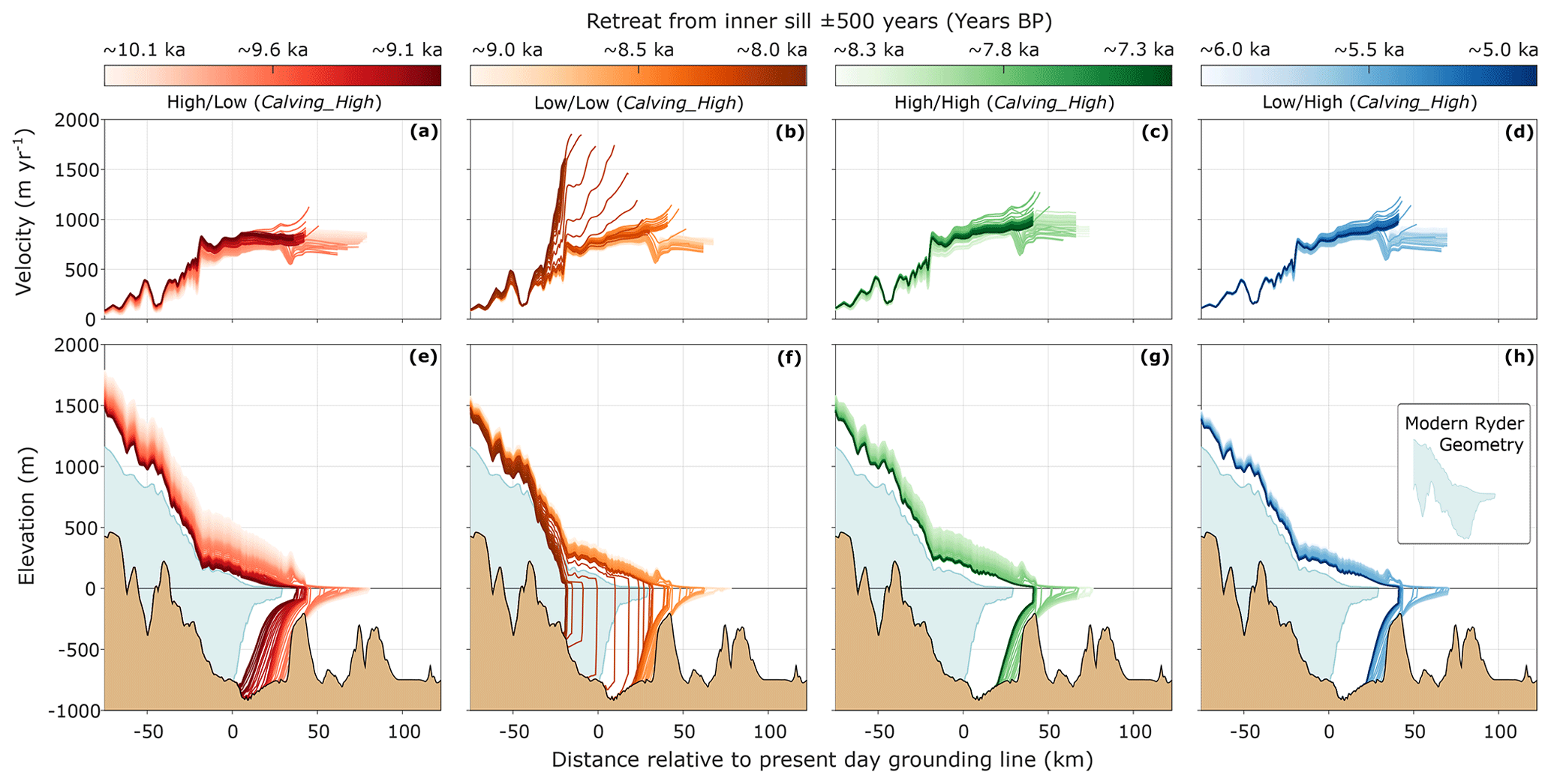
Figure 7 Ice dynamics of Ryder Glacier in the 500 years prior to and after retreat from the inner sill in Sherard Osborn Fjord for all transient runs forced with the Calving_High ocean scenario. (a–d) Changes in velocity along the centre flowline. (e–h) Changes in the geometry of Ryder Glacier using 2D cross sections from the centre flowline.

4.1.2 Holocene minimum and ice tongue collapse

Ryder Glacier's Holocene minimum extent is captured by the sediment unit LU3 found throughout sediment cores taken in Sherard Osborn Fjord and spanning 6.3±0.3 to 3.9±0.4 ka BP. This unit marks a period of low sedimentation and the presence of IRD, interpreted by O'Regan et al. (2021) as the collapse of the ice tongue and the retreat of the glacier into the restricted embayment ∼40 km upstream of the contemporary grounding line position (Fig. 2a).

None of our transient Holocene simulations match, in detail, this hypothesised retreat to the restricted embayment (Fig. 6). We simulate a maximum retreat of Ryder Glacier to just in front of the restricted embayment, ∼25 km behind the present-day grounding line position (Fig. 5). A retreat to this position occurs in all simulations using the Reference ocean forcing with the exception of the run using the mildest SMB scenario Low/High (Fig. 5a). Timing of retreat again follows the same pattern of SMB, with a Holocene minimum occurring at 7.9 ka BP for SMB High/Low, 7.1 ka BP for Low/Low, 6.4 ka BP for High/High ka BP and 4.5 ka BP for Low/High.

The same timing and extent of retreat are also found in the Calving_High and Calving_Low scenarios, with the exception of run Low/Low (Calving_High) that retreats ∼900 years earlier (8 ka BP) than its Reference run due to the collapse of the floating tongue (Fig. 7). For Melt_Low simulations, a similar Holocene minimum position of ∼25 km behind the present-day grounding line is reached with High/Low and Low/Low SMB scenarios, albeit later than their Reference ocean simulations, while High/High (Melt_Low) does not retreat past the present-day grounding line (Fig. 5a and b). All runs using the Melt_High ocean forcing retreat to this common Holocene minimum position, but again retreat is found to be both faster and more concentrated, with a minimum extent of Ryder reached between 9.5 and 6.5 ka BP.

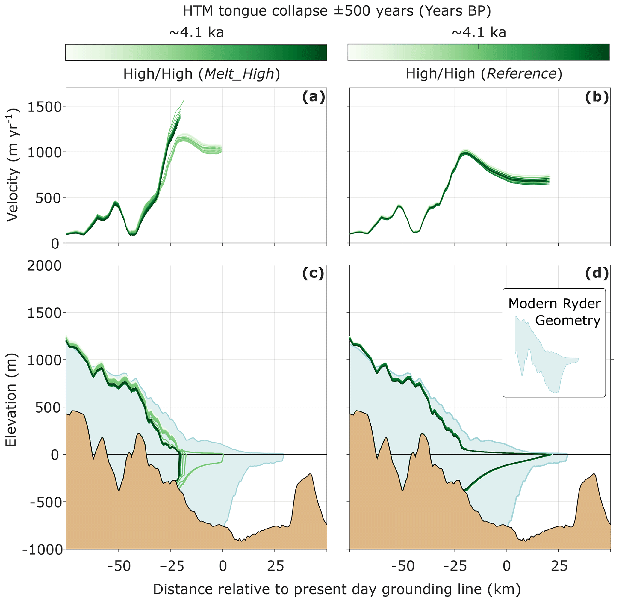
Figure 8 Ice dynamics in the 500 years prior to and after the loss of the floating tongue during the transient run High/High (Melt_High) and ice dynamics of the High/High (Reference) during the same period. (a–b) Change in velocity along the centre flowline. (c–d) Change in the geometry of Ryder Glacier using a 2D cross section from the centre flowline.

We find Ryder's floating tongue collapses during our Holocene simulations in two distinct manners. The first occurs when Ryder retreats from the inner sill (ca. at km 40 in Fig. 7). This happens in both runs using the High ocean forcing as well as Low/Low (Calving_High). Figure 7 compares the retreat of all four Calving_High simulations for the 500 years before and after the grounding line detaches from the inner sill. Runs forced with SMB scenarios High/Low, High/High and Low/High follow the same pattern of behaviour, albeit the timing of retreat differs. Therein, Ryder's retreat from the inner sill is followed by a steady grounding line retreat of between 20 and 30 km in the following 500 years (Fig. 7e, g and h). Terminus velocities prior to the retreat from the sill are ∼750 m yr⁻¹, increasing to >1000 m yr⁻¹ as the grounding line retreats from the bathymetric high, before gradually subsiding below 1000 m yr⁻¹. Run Low/Low (Calving_High) initially follows the same behaviour; however, large calving rates which remove the majority of the floating tongue coincide with an acceleration of terminus velocities to ∼1900 m yr⁻¹ and the glacier retreats as a sheer cliff face 35 km in ∼40 years (Fig. 7b and f). The glacier then rests at its Holocene minimum as a grounded tidewater glacier, with terminus velocities of ∼1600 m yr⁻¹.

The second mechanism for tongue collapse occurs in all runs forced with the Melt_High ocean scenario. This behaviour is exemplified in Fig. 8 by run High/High (Melt_High) where the glacier, with the grounding line already at its Holocene minimum, sees its 25 km tongue disintegrate and terminus velocities accelerate from ∼1000 to ∼1500 m yr⁻¹. No further grounding line retreat is observed, as the glacier remains in shallow waters in front of the restricted embayment. The timing of collapse varies depending on SMB scenarios: High/Low at 7.5 ka BP, Low/Low at 6.2 ka BP, High/High at 4.1 ka BP and finally Low/High at 2.1 ka BP. The collapse behaviour is contrasted by the use of the Reference ocean forcing in High/High (Reference) (Fig. 8b and d), where a floating tongue of almost 50 km in length is sustained throughout the Holocene and velocities at the terminus remain consistently between 600 and 700 m yr⁻¹.

4.1.3 Neoglacial regrowth

The final lithologic units found in Sherard Osborn Fjord, beginning at 3.9±0.4 ka BP, are characterised by increased sedimentation rates and the deposition of laminated sediments, marking the advance of the grounding line and the eventual regrowth of Ryder's ice tongue towards its LIA maximum (Fig. 2b).

In our transient simulations, we only find a late Holocene readvance of the grounding line using the Melt_Low or extreme Low ocean forcing (Fig. 5b and f). Therein, the most pronounced readvance occurs in the Low/Low (Melt_Low) run where the grounding line migrates ∼25 km. The readvance is more subtle in runs High/Low (Melt_Low) and High/High (Melt_Low) at ∼10 km, although substantial thickening upstream of the grounding is observed (Fig. 6k and o). This same pattern of thickening is observed in runs Low/High (Melt_Low) and Low/High (Low), although the grounding line, which has not retreated from the inner sill during the HTM, does not show any advance. In all aforementioned runs, the floating tongue advances into Sherard Osborn Fjord at a similar rate to grounding line migration. In runs where the grounding line does not readvance, such as those using the Reference ocean scenario (Fig. 6i and m), there is no increase in length of the floating tongue towards the LIA maximum. Furthermore, there is no regrowth of the floating tongue in runs where a collapse occurs in the mid-Holocene (Fig. 6j and n).

4.2 Terrestrial Holocene evolution

Here we explore the evolution of the terrestrial ice-sheet margin during our simulations in the context of reconstructed ice-sheet isochrones found in the PaleoGrIS database (Leger et al., 2024). Firstly, we assess the simulated retreat of the ice-sheet margin during the early Holocene from 10 ka to 8 ka BP (Sect. 4.2.1), over which time our model domain transitions from nearly entirely ice covered to roughly the same ice coverage as found at present-day (Fig. S4). 8 ka BP also marks a pause in ice retreat found across all our simulations, likely relating to the Warming Land Stade inferred by Kelly and Bennike (1992) (Fig. S4). Furthermore, we describe the neoglacial advance of the ice-sheet margin by comparing a minimum ice extent, taken at 6 ka BP for all runs except those forced with SMB scenario Low/High when the minimum occurs later at 4 ka BP (Fig. S4), with the final state of our simulation representing the present day (Sect. 4.2.2).

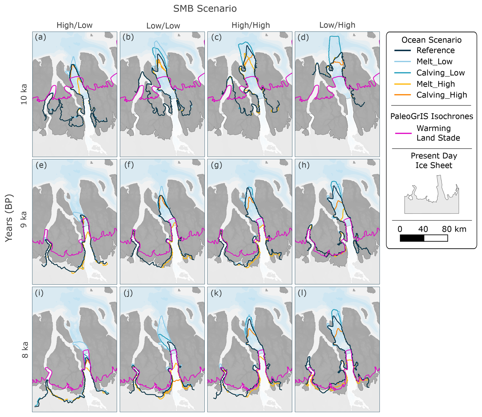
Figure 9 Evolution of the ice-sheet margin in the model domain at 10 (a–d), 9 (e–h) and 8 ka BP (i–l). The various SMB scenarios are grouped into columns, while coloured ice-sheet margins depict the ocean scenario used in each simulation: Reference, navy; Melt_Low, light blue; Calving_Low, blue; Melt_High, light orange; and Calving_High, dark orange. Purple lines represent the reconstructed ice-sheet margins from the PaleoGrIS database (Leger et al., 2024).

4.2.1 Warming Stade retreat

Retreat rates of the terrestrial ice margin vary considerably with the choice of SMB scenario (Fig. 9). The most negative SMB scenario, comprised of high temperature and low precipitation (High/Low), produces an ice margin that is consistently 30–40 km behind the reconstructed margin from the geological archive (Fig. 9a, e and i). The ice margins from simulations using the Low/Low (Fig. 9b, f and j) and High/High (Fig. 9c, g and k) SMB scenarios follow a similar retreat rate during the early Holocene yet still exceed the rate of retreat from reconstructed isochrones across Warming Land despite more closely matching the retreat around Steensby Glacier and Saint George Fjord. Finally, simulations using the least negative SMB scenario, containing low temperature and high precipitation (Low/High), produce a retreat that tracks the reconstructed isochrone especially well at 9 and 8 ka BP, despite producing a slightly slower retreat at 10 ka BP (Fig. 9d, h and l).

While the reconstructed ice margins from the PaleoGrIS database provide valuable insights into the Holocene extent of GrIS, we note that the isochrones across northern Greenland are rated with low confidence, the third lowest of four confidence levels discussed in Leger et al. (2024). This is due to the sparse number of radiocarbon ages and the almost complete lack of exposure event ages across the region. Nevertheless, the series of moraines that have been dated in northern Greenland show a standstill in Holocene retreat between 9 and 8 ka BP and indicate that the ice sheet had not yet retreated behind its modern-day extent (Fig. 1; Kelly and Bennike, 1992). This underscores that the retreat of the ice margin in the most negative SMB scenario High/Low is too pronounced, with the simulated ice margin already behind the present-day ice sheet by 9 ka BP.

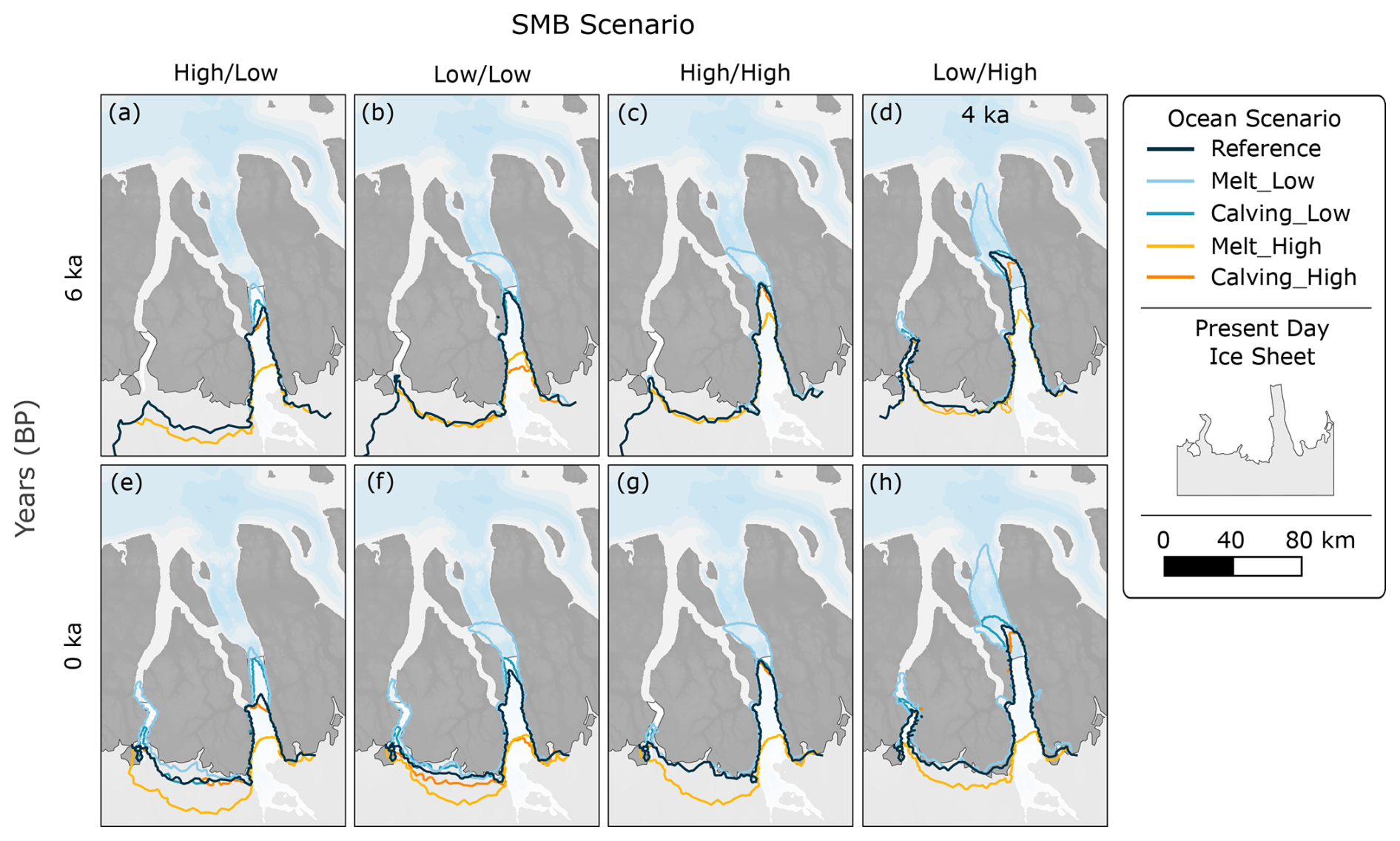
Figure 10 Comparison of the ice-sheet margin at the Holocene minimum (a-d) and the end of our simulations representing the present day (e–h). The various SMB scenarios are grouped into columns, while coloured ice-sheet margins depict the ocean scenario used in each simulation: Reference, navy; Melt_Low, light blue; Calving_Low, blue; Melt_High, light orange; and Calving_High, dark orange.

4.2.2 Holocene minimum and regrowth

The minimum glaciated extent of the model domain during the transient Holocene runs is shown in Fig. 10a–d. The terrestrial margin, on both Warming Land and Wulff Land, has retreated behind that of the present-day ice sheet in all simulations. There is little variation in the ice margin across the different ocean scenarios used for runs forced with Low/Low, High/High and Low/High SMB scenarios, with the simulated ice-sheet minimum sitting between 10 and 20 km behind the contemporary ice margin on Warming Land. For simulations using the High/Low SMB, modelled retreat is greater, with the margin retreated at least 30 km behind the present-day ice sheet and Steensby Glacier withdrawing from Saint George Fjord. Furthermore, simulation High/Low (Melt_High) produces a retreat that is 10 km further in land than all other ocean forcings.

Regrowth of the terrestrial margin towards its present-day location occurs in all our simulations with the exception of those using the Melt_High ocean scenario (Fig. 10e–h). For such simulations, the ice-sheet margin remains almost unchanged from its Holocene minimum position, 20–40 km behind the present ice sheet depending on the chosen SMB scenario. All remaining runs using the High/High and Low/High SMB scenarios, both containing the high-precipitation pathway, end with an ice-sheet margin that is very consistent with the present-day ice sheet across both Warming Land and Wulff Land. For SMB scenarios High/Low and Low/Low there are variations in the final position of the ice front depending on the chosen ocean forcing; however, all simulations produced a final ice margin that is within 10 km of the contemporary ice sheet.

5 Discussion

We have simulated the Holocene evolution of Ryder Glacier across different plausible atmospheric- and oceanic-forcing scenarios with the glacier's terminus position and ice dynamics constrained by marine and terrestrial proxy records. In summary, we find that variations in SMB have a distinct impact on timings of retreat for terrestrial and marine ice-sheet margins. The climate pathway built from low temperature and high precipitation (Low/High) matches the early Holocene terrestrial retreat across our domain best, in contrast to the most extreme scenario of high temperature and low precipitation (High/Low), which produces retreat that far exceeds the rate found in the terrestrial record (Fig. 9). For the marine margin of Ryder, enhanced ocean melt plays a key role in driving grounding line retreat to match the sediment archive in all but the most extreme SMB scenario (Fig. 5). Moreover, ocean melt is crucial to initiate the collapse of Ryder's ice tongue in the HTM (Fig. 8), while the readvance of the grounding line towards its modern-day position only occurs with subdued ocean melt forcing (Fig. 5b). Furthermore, the variations in the calving threshold have a minimal impact during the early Holocene retreat, likely due to the continued presence of the floating tongue, with its stability aided by the narrowing of Sherard Osborn Fjord. The major components influencing Ryder Glacier's behaviour in our simulations will be discussed in more detail below.

5.1 Holocene warming and the importance of precipitation

Atmospheric changes, associated with the pronounced shifts in surface temperatures and precipitation from the YD into the Holocene, exerted a first-order control on the behaviour of Ryder Glacier in our simulations. This is clear from the initial homogeneous retreat, >10 ka BP, found across all simulations in response to an abrupt rise in temperature and independent of the choice of ocean forcing. Subsequent variations in temperature and precipitation led to heterogenous retreat rates during the Holocene, yet the choice of SMB scenario provides a consistent pattern of retreat across all ocean forcings, ranging from the most extreme SMB scenario of high temperature and low precipitation to the mildest scenario of low temperature and high precipitation. We find that this mildest SMB scenario produces a terrestrial ice margin that fits best with reconstructed ice-sheet positions in the geologic records (Fig. 9). Furthermore, precipitation exerts substantial control in modulating mass loss during the early Holocene in our simulations, so much so that SMB scenarios using the low-precipitation pathways produce the fastest retreat rates of both the grounding line and terrestrial ice margins (Figs. 5 and 9). This suggests that when the catchment of Ryder Glacier was deprived of snowfall, the grounding line retreated. These results contrast Holocene modelling studies of southwestern Greenland, where variations in temperature played a greater role in determining retreat rates (Briner et al., 2020; Cuzzone et al., 2022).

We attribute the strong impact of precipitation during the Holocene to the environmental characteristics of northern Greenland. The region, in its contemporary setting, experiences some of the lowest precipitation rates found on the ice sheet (Box, 2013; McIlhattan et al., 2020), owing both to its distance from major open-water bodies, as the nearby Arctic Ocean is sea ice covered, and to cooler temperatures at extreme latitudes. Consequently, northern Greenland is especially vulnerable to rapid atmospheric warming (Noël et al., 2019). Reconstructed early Holocene precipitation suggests lower-than-modern rates of accumulation (Fig. 3b), hinting that North Greenland was highly sensitive to early Holocene warming. Biomarker analysis of sediment cores in the Lincoln Sea suggests that the period between about 11.3 and 9.7 ka BP may have experienced seasonal sea ice, implying nearby open-water conditions during summers (Detlef et al., 2023). However, it is not known whether such conditions in the Lincoln Sea directly affected precipitation over the North Greenland Ice Sheet. The sediment core study further suggests a maintained perennial sea ice cover in the southern Lincoln Sea throughout the reminder of the Holocene. In contrast, towards the mid-Holocene, reduced sea ice extent in Baffin Bay and the Labrador Sea, together with warmer temperatures, are thought to have brought greater-than-modern-day levels of accumulation to northern Greenland (Thomas et al., 2016). Such reasoning has been invoked to explain the readvance of valley glaciers and the sustained presence of local ice caps across northern and northeastern Greenland during the HTM (Möller et al., 2010; Larsen et al., 2016, 2019), while simulations of Hans Tausen Iskapp showed that precipitation rates higher than modern-day values were crucial in buffering higher temperatures during the HTM and ensuring the survival of the ice cap (Zekollari et al., 2017). Greater-than-modern-day precipitation rates are only found in our high-precipitation scenario (Fig. 3b), which coupled with a low-temperature pathway produced the most accurate retreat of terrestrial margin during the early Holocene (Fig. 9).

5.2 Submarine melt drives inner fjord retreat

Whilst a negative trend in SMB is the overall dominant driver of Ryder Glacier's Holocene retreat, our results indicate that ice–ocean interactions played an increasingly important role as the interglacial progressed. The ocean melt rate is particularly important for the grounding line's retreat from the inner sill in Sherard Osborn Fjord, where our simulations produce a wide range of retreat dates spanning from 9.4 to 5.4 ka BP (Fig. 5). The study of O'Regan et al. (2021) shows that sedimentation on the inner sill, and thus the beginning of grounding line retreat, began at 9.3±0.4 ka BP. We find that using a modern Reference ocean melt rate our simulations are only able to match this timing of retreat when using the most negative SMB scenario (High/Low (Reference); Figs. 5a and 6e). Such an extreme SMB scenario leads to a terrestrial retreat that is significantly faster than that found in reconstructed isochrones (Fig. 9). Other, more moderate, SMB scenarios result in grounding line evolutions lagging behind the sediment record when using Reference ocean melt forcings, with retreat from the inner sill not beginning until 8.3 ka BP (Figs. 5a and 6e). It is only when using a High_Melt ocean parameterisation that all SMB scenarios yield grounding line retreats that are in line with the marine record (Figs. 5c and 6f).

The inner sill has a ∼6.2 km wide central zone with a modern depth of ∼300 m (Jakobsson et al., 2020). Ocean melt rates at the grounding line atop the inner sill in our melt parameterisation would peak at 26.6 m yr⁻¹ for the Reference ocean scenario and 66.6 m yr⁻¹ for the High_Melt simulations, with the latter exceeding the modern melt rates seen under contemporary Greenlandic floating tongues with their grounding lines in much deeper waters (Wilson et al., 2017; Millan et al., 2023). Although the depth of the modern inner sill impedes the flow of warm AW (Jakobsson et al., 2020), relative sea level (RSL) estimates from ∼8 ka BP indicate the sill to be between 40 and 80 m deeper than present (Lecavalier et al., 2014; Glueder et al., 2022), likely allowing AW to reach the paleo grounding line of Ryder Glacier, and drive higher melt rates that otherwise would not be possible in shallower, cooler waters. Cronin et al. (2022) discuss the evidence for the existence of such warm waters in the Lincoln Sea at the mouth of Sherard Osborn Fjord throughout the entire Holocene from a benthic ostracod and foraminifera assemblage. In particular, they point to a pronounced AW signal between 8.5 and 6 ka, which is close in time to the beginning of sedimentation on the inner sill. This stresses that the presence of warm AW in the fjord may have been crucial for the retreat of the grounding line from the sill. The presence of such warm waters around Greenland during the Holocene is well documented (Jennings et al., 2006; Pados-Dibattista et al., 2022) and has been indirectly linked to the collapse of the neighbouring Petermann Glacier ice tongue during the HTM (Reilly et al., 2019). Furthermore, similar Holocene modelling studies at Jakobshavn Isbræ (Kajanto et al., 2020) and the Northeast Greenland Ice Stream (Tabone et al., 2024) also show that pronounced increases in ocean temperatures were required to force grounding line retreat from stable bathymetric highs in order to align with geological records.

Ocean melt rates were crucial to the stability of Ryder's floating tongue during the HTM. Our simulations produce a complete break-up of the ice tongue in two distinct manners: first during the early Holocene as the glacier retreats from the inner sill into deeper waters (Fig. 7) and second during the mid-Holocene once the grounding line has already retreated into the shallower waters upstream of the present grounding line (Fig. 8). The sediment facies that depict the collapse of Ryder's floating tongue, LU3 (6.3±0.3 to 3.9±0.4 ka BP), are dated ∼3 ka years after Ryder's retreat from the inner sill, LU5 (9.3±0.4 to 7.6±0.40 ka BP). The presence of LU4 (7.6±0.40 to 6.3±0.3 ka BP), a faintly laminated facies that lacks evidence of bioturbation, suggests that Ryder maintained its floating tongue for a substantial period of time as the grounding line retreated away from the inner sill (O'Regan et al., 2021). We therefore argue that the collapse of Ryder's tongue is best captured in runs using the High_Melt scenario, wherein Ryder retreats steadily through the overdeepened part of the fjord behind the inner sill, while continuing to be buttressed by a floating tongue, towards its Holocene minimum position. In this scenario, elevated melt rates result in a shortened floating tongue that weakens the glacier's ability to buttress interior ice, thus driving an increase in ice velocities and calving until its eventual collapse (Fig. 8).

5.3 Ryder's floating tongue was pivotal in its Holocene evolution

Mass loss through calving has played a key role in the recent evolution of the GrIS and is projected to play a vital role in the coming century (Goelzer et al., 2020; Choi et al., 2021). Yet, such processes are often not explicitly included in paleo-modelling efforts owing to the computational costs associated with high-resolution grids needed to accurately simulate fast-flowing ice streams and their associated calving dynamics. Here, we build on the findings of Cuzzone et al. (2022), who included a similar calving set-up when simulating the Holocene retreat of Kangiata Nunaata Sermia, southwestern Greenland. Cuzzone et al. (2022) note how the inclusion of calving allowed the marine margins to persist longer in the fjords, relative to adjacent terrestrial ice, due to a greater transport of mass from the interior, which in turn led to thinning in the upper regions of the domain. We find such consistencies across our simulations during the early Holocene, where, despite rapid retreat of the terrestrial ice, Ryder Glacier maintains an extended position in the fjord (Fig. 9).

In our simulations, variations to the calving threshold have minimal influence on the grounding line evolution and inland thinning of Ryder Glacier (Figs. 5a, d, and e and S3). We attribute this to the sustained presence of an ice tongue during the Holocene retreat, suppressing calving and discharge. When we simulate a collapse of the ice tongue, either during retreat from the inner sill (Fig. 7) or at Ryder's Holocene minimum (Fig. 8), the loss of buttressing and transition to calving from an unconstrained grounded front leads to an increase in ice discharge and inland thinning. Our results indicate that Ryder's floating tongue was present during the entire >4000-year retreat from the outer sill, stabilising the glacier and modulating ice discharge until its collapse at the glacier's Holocene minimum position. This long-term stability was likely supported by the geometry of Sherard Osborn Fjord, which continually narrows from the outer sill towards a 10 km wide bottleneck that extends 40 km south from the inner sill (Fig. 2). This region has been linked to the stability of the contemporary ice tongue and calving front (Holmes et al., 2021), where narrowing fjord walls increase lateral drag, modulating grounding line retreat and, crucially, floating tongue stability (Åkesson et al., 2018b; Frank et al., 2022). The bottleneck likely allowed Ryder's ice tongue to outlast the floating extension at the neighbouring Petermann Glacier, which collapsed at 6.9 ka BP only ∼600 years into the glacier's retreat from the outer sill in Petermann Fjord, after which the fjord's geometry begins to deepen and, crucially, widen (Reilly et al., 2019). With the collapse of Nioghalvfjerdsbræ (79N) occurring even earlier, by 8.5 ka BP (Smith et al., 2023), it is very likely that Sherard Osborn Fjord contained the last major floating extension from the Greenland Ice Sheet during the deglaciation from the LGM.

The heightened discharge from a collapse of the floating ice tongue at Ryder restricts any readvance of the terrestrial and marine margins during the late Holocene (Figs. 6n and 10). This implies that a shift in calving dynamics, driven by the regrowth of the ice tongue and increased buttressing, was crucial to the readvance of Ryder glacier during the late Holocene. Although our experimental set-up does not account for transiently evolving ocean forcings, the lack of ice tongue regrowth across all SMB scenarios indicates that cooling atmospheric temperatures alone are not sufficient for the regrowth of the floating terminus and that a reduction in ocean melt rate and/or a reduction in calving owing to the formation of a rigid ice mélange was required. This aligns with the results of Åkesson et al. (2022), who found that a decrease in both ocean melt and calving was required to regrow Petermann Glacier's ice tongue in the event of any collapse as well as work by Kajanto et al. (2024), where a decrease in calving rate was required to re-form the ice tongue of Jakobshavn Isbræ and readvance the grounding line to the glacier's LIA position.

Our findings emphasise the role of floating tongues in controlling ice discharge over centennial and millennial timescales and stress the importance of including both floating ice and calving dynamics when undertaking paleo-modelling studies of the GrIS. This is especially pertinent to northern Greenland, where ice streams at the LGM were thought to have coalesced and formed ice shelf conditions into the Lincoln Sea (Dawes, 1986; Larsen et al., 2010) before collapsing during the HTM and then regrowing in the late Holocene to exert an important buttressing force on ice flow from the GrIS interior. Continental-scale model reconstructions of the GrIS during the Holocene which omit the inclusion of floating ice and calving, or do not have the required model resolution to capture grounding line dynamics in narrow Greenlandic fjords, may lack the required fidelity to accurately simulate the ice-sheet's evolution (Simpson et al., 2009; Lecavalier et al., 2014).

While we have discussed the importance of fjord geometry and bathymetry to the evolution of Ryder Glacier, we acknowledge that one of the limitations of our experimental set-up is the lack of transient RSL changes during the Holocene. Despite this, we tentatively assume that including such dynamics would not have a significant impact on our model results, taking note from a similar Holocene study of Jakobshavn Isbræ by Kajanto et al. (2020), which found RSL changes had minimal impact on the in-fjord retreat as such variations are small compared to fjord depth. Although the coalescing of the Greenland and Innuitian ice sheets brought RSL ∼80 m higher at the beginning of the Holocene (Lecavalier et al., 2014; Glueder et al., 2022), the pronounced depths of Sherard Osborn Fjord mean it is likely that any influence would have been restricted to the shallow inner sill as discussed in Sect. 5.2. Future work, which will aim to simulate the Holocene deglaciation of the entire northern sector of the GrIS, will include RSL variations through new solid earth feedbacks currently being implemented in ISSM or through prescribed forcings of sea level changes from prior research (e.g. Caron et al., 2018).

5.4 Ryder Glacier in the future

The retreat of Ryder to its HTM minimum provides a crucial analogue to understand how the glacier will evolve when confronted with sustained temperatures above pre-industrial levels. Our simulations indicate that both atmosphere–ice and ocean–ice interactions will dictate Ryder's future behaviour. At present, Ryder's floating tongue and grounding line sit within the bottleneck of Sherard Osborn Fjord, providing significant buttressing and stability. The calving front has remained unmoved for half a century, owing to fjord geometry (Holmes et al., 2021). If the ice tongue at Ryder persists, the grounding line will undergo a steady retreat along the prograde topography inland of its current position, with the speed of retreat a function of both SMB and submarine melt, with the latter able to weaken the floating tongue's ability to buttress, leading to enhanced discharge (Fig. 8). Despite being shielded from warm AW by the shallower inner sill (Jakobsson et al., 2020), melt rates at the grounding line of Ryder have increased in recent decades while the floating tongue has thinned (Millan et al., 2023). Submarine melt is not just a product of ocean heat, but also turbulent processes at the ice–ocean interface that are linked to the upwelling of buoyant plumes fed by the discharge of fresh water at the grounding line (Slater and Straneo, 2022). At Nioghalvfjerdsbræ (79N), Greenland's largest floating terminus that is also shielded from warm AW by a bathymetric high (Hill et al., 2017; An et al., 2021), extreme melt rates of 100 m yr⁻¹ have been linked to increased subglacial discharge from enhanced surface melt (Zeising et al., 2024). Rising melt rates at Ryder have coincided with a substantial increase in supraglacial lakes on the glacier (Otto et al., 2022), the build-up and drainage of which are likely to deliver an increased flux of fresh water to the grounding line that will lead to a greater transfer of heat from the ocean to the glacier. Therefore, despite the protection offered by the inner sill in Sherard Osborn Fjord, ocean melt is set to play a crucial role in both the grounding line retreat and tongue stability of Ryder Glacier into the future.

During the HTM, Ryder retreated inland of its present position. The most common Holocene minimum position achieved in our simulations is ∼25 km behind the modern-day grounding line, in relatively shallow waters (∼300 m deep) and in front of the restricted embayment (Figs. 6 and 8). The ever-decreasing marine ice thickness heightens the role of atmosphere–ice interaction and indicates that further retreat would require a greater negative trend in SMB. This is best exemplified in both runs using the extreme High ocean forcings which retreat to their Holocene marine minimum by 9 ka BP (Fig. 6h), only to remain unmoved during the HTM. While we are unable to match the grounding line retreat into the restricted embayment hypothesised by O'Regan et al. (2021), the inherent uncertainties in SMB reconstructions over the Holocene mean that further retreat from our simulated position cannot be ruled out in a HTM-like climate. However, owing to the substantial thickness of simulated inland ice, we believe that it is unlikely that Ryder retreated significantly further and became entirely terrestrial during the Holocene. Instead, it appears that Ryder remained a marine-terminating glacier during the HTM, with the grounding line in shallow waters in front of or in the restricted embayment. This implies that under a future climate that resembles the HTM, Ryder will retain its connection to the ocean and will continue to contribute to global sea level rise through both runoff and discharge.

6 Conclusions

Geological evidence from terrestrial and marine settings can provide valuable insights into the evolution of ice sheets across glacial–interglacial cycles at snapshots in time. Coupling such knowledge with ice-sheet models allows for continuous insight into the long-term evolution of ice sheets. Here, we employed a high-resolution 3D thermomechanical ice-sheet model to explore the evolution of Ryder Glacier throughout the Holocene. By focusing on a single outlet glacier from the GrIS, we were able to run our model at mesh resolutions <1 km to both accurately simulate grounding line dynamics and disentangle the influence of ice–ocean and ice–atmosphere interactions. We find the following:

• Rapid retreat of the ice margin in the early Holocene was driven by substantial climatic warming. The retreat of the terrestrial and marine ice margins is independent of the prescribed ocean forcing during the transition out of the YD until ∼10 ka BP.

• Precipitation rates played a key role in modulating both the pace and magnitude of retreat, likely reflecting the arid nature of northern Greenland. We find that the climate scenario where mid-Holocene precipitation rates exceed that of contemporary levels produces terrestrial ice retreat that best matches the geologic record.

• After ∼10 ka BP, submarine melt begins to influence the retreat of the marine margin of Ryder Glacier in all but the most negative SMB scenario. Heightened submarine melt rates were crucial in retreating Ryder from a stable position on the inner sill as well as inducing the collapse of the ice tongue during the HTM.

• Before its collapse, the paleo-ice tongue at Ryder Glacier was crucial in modulating ice loss during the early Holocene, particularly during Ryder's retreat from the inner sill into a large overdeepening in Sherard Osborn Fjord. We link the ice tongue's stability and influence to the 10 km wide bottleneck in Sherard Osborn, where the contemporary ice tongue and grounding line currently lie.

• Regrowth of the ice tongue was crucial to the readvance of the terrestrial and marine ice margins during the late Holocene cooling. Changes in SMB alone cannot explain the re-formation of the tongue, indicating that cooling ocean temperatures and reduced calving rates were required.

Although changes in SMB may dictate large-scale ebbs and flows in ice-sheet margins, ice–ocean interactions can play a significant role in the evolution of marine outlet glaciers, and thus discharge from ice sheets, across extended timescales of centuries and millennia. By running Holocene simulations of Ryder Glacier we provide vital analogues for the future evolution of the glacier in a warming climate, stressing both the continued importance of the ice tongue in buttressing ice flow and the role of submarine melt in weakening the ice tongue and driving grounding line retreat.