Wind and topography underlie correlation between seasonal snowpack, mountain glaciers, and late-summer streamflow

In a warming climate, net mass loss from perennial snow and ice (PSI) contributes a temporary source of unsustainable streamflow. However, the role of topography and wind in mediating the streamflow patterns of deglaciating watersheds is unknown. We compare lidar surveys of seasonal snow and PSI elevation change for five adjacent watersheds in the Wind River Range, Wyoming (WRR). Between 2019 and 2023, net mass loss from PSI is equivalent to ∼ 10 %–36 % of August–September streamflow. Across 338 manually classified PSI features >0.01 km², glaciers contribute 68 % of the total mass loss, perennial snowfields contribute 8 %, rock glaciers contribute 1 %, buried ice contributes 6 %, and the remaining 17 % derives from semi-annual snowfields and small snow patches. Surprisingly, watersheds with more area-normalized seasonal snow produce less late-summer streamflow ($r=-\mathrm{0.60}$), but this correlation is positive (r=0.88) considering only deep snow storage (SWE > 2 m). Most deep snow (87 %) is associated with topography that is conducive to wind drift formation. Deep seasonal snow limits the mass loss contribution of PSI features in topographic refugia. We show that watersheds with favorable topography exhibit deeper seasonal snow, more abundant PSI features (and hence greater mass loss in a warming climate), and elevated late-summer streamflow. As a result of deep seasonal snow, watersheds with the most abundant PSI would still produce 45 %–78 % more late-summer streamflow than nearby watersheds in a counterfactual scenario with zero net mass loss. Similar interrelationships may be applicable to mountain environments globally.

1 Introduction

Climate warming reduces snow and ice storage in mountain environments, disrupting historical water supply timing and affecting downstream ecosystems (Milner et al., 2017; Drenkhan et al., 2023). Seasonal snow storage (i.e., snow that accumulates and melts each year) provides a seasonal buffer between the timing of precipitation and runoff (Barnett et al., 2005; Stewart et al., 2005; Li et al., 2017; Gordon et al., 2022). Perennial snow and ice (PSI) features, including glaciers, perennial snowfields, rock glaciers, and buried ice, collectively provide a decadal- to century-scale buffer that reduces interannual streamflow variability between wet and dry years (Meier, 1969; Fountain and Tangborn, 1985; Moore, 1992; Pohl et al., 2017; van Tiel et al., 2020). However, climate warming is causing earlier seasonal snowmelt and driving glacier recession globally, which reduces the warm-season streamflow volume and increases the temporal variability of downstream water supplies (Oerlemans, 1986; Zemp et al., 2009; Huss, 2012; Zemp et al., 2015; Brun et al., 2017; Huss et al., 2017; Shean et al., 2020; Hugonnet et al., 2021). Earlier snowmelt and glacier recession both contribute to the snow–albedo feedback by reducing landscape albedo, which increases the energy available for melt and further accelerates the reduction of snow and glacier storage (Johnson and Rupper, 2020; Di Mauro and Fugazza, 2022; Davies et al., 2024). This feedback process is a driver of elevation-dependent warming (McGuire et al., 2012; Rangwala and Miller, 2012; Pepin et al., 2015; Palazzi et al., 2019). Glacier recession poses challenges for socio-hydrologic adaptation in downstream communities (Kaser et al., 2010; Carey et al., 2017; Drenkhan et al., 2023). With reduced seasonal snow and fewer PSI features to buffer precipitation variability, mountain watersheds are increasingly vulnerable to hydrological extremes, including snow drought (Harpold et al., 2017; Dierauer et al., 2019; Huning and AghaKouchak, 2020).

Rough mountain topography can sustain PSI features at or below the regional equilibrium line altitude (ELA, where mean annual snow accumulation equals ablation) due to wind drifting, avalanches, and topographic shading, making it difficult to generalize mass balance patterns across a mountain landscape (Kuhn, 1995; Allen, 1998; Hoffman et al., 2007; Hughes, 2010; Florentine et al., 2018, 2020). Estimates of mountain PSI mass loss at the landscape scale are generally based on remote sensing (e.g., Bamber and Rivera, 2007) or extrapolation (e.g., Huss, 2012). Optical remote sensing is useful for mapping spatial patterns of seasonal snow persistence and PSI extent (Meier, 1980; Selkowitz and Forster, 2016; Hammond et al., 2018), but imagery-based techniques do not provide a direct estimate of mass or volume changes. Repeat surveys using lidar (light detection and ranging) can quantify elevation changes caused by snow accumulation and PSI ablation, constraining the spatial variability and timing of PSI mass loss (Sold et al., 2013; Helfricht et al., 2014).

Net mass loss from PSI features can contribute a considerable fraction of streamflow in alpine regions (Schaner et al., 2012; Bliss et al., 2014; Huss and Hock, 2018), and reducing uncertainty in the PSI mass loss contribution to streamflow is important to constrain the climate vulnerability of the mountain water supply. PSI mass loss temporarily increases mountain streamflow by providing an additional source of late-summer meltwater (Lambrecht and Mayer, 2009; Huss and Hock, 2018). However, this increased streamflow is unsustainable because PSI features are finite, ultimately leading to streamflow reductions (Stahl and Moore, 2006; Nolin et al., 2010; Moore et al., 2020; Rets et al., 2020). The fractional mass loss contribution to annual streamflow depends on the relative volume of meltwater contributed by net mass loss versus annual precipitation (O'Neel et al., 2014).

The impact of deglaciation on mountain streamflow patterns is confounded by spatial patterns of seasonal snow persistence. Seasonal snow persistence is a primary driver of hydrograph shape and streamflow volume in snowy alpine watersheds (Hall et al., 2012; Richer et al., 2013; Barnhart et al., 2016; Hammond et al., 2018). The hydrograph shape represents the timing of water availability, which is of paramount importance in regions with limited artificial storage capacity (McNeeley et al., 2018; Siirila-Woodburn et al., 2021; Gordon et al., 2024). The presence of PSI results from historic snow accumulation exceeding melt, so PSI features necessarily coincide with the most persistent areas of the seasonal snowpack. PSI features also mediate snowmelt runoff timing (Fountain and Tangborn, 1985; Fountain, 1996; Fleming and Clarke, 2005), so it can be challenging to attribute seasonal hydrograph shape and inter-watershed variability exclusively to differences in seasonal snowmelt or PSI mass loss (Frenierre and Mark, 2014; Brahney et al., 2017). Paired watershed studies with variable PSI abundance can provide compelling evidence for the role of PSI features in shaping the downstream hydrograph (Hood and Berner, 2009; Bell et al., 2012; Kneib et al., 2020; Zhou et al., 2021). However, the causal relationship between snow persistence and PSI abundance complicates the interpretation of space-for-time studies of deglaciation, where nearby watersheds with fewer glaciers are used as a proxy for the future of deglaciating watersheds (Bell et al., 2012). The persistence of cold-water-stream species after deglaciation supports the role of seasonal snow in sustaining alpine streamflow patterns (Muhlfeld et al., 2020), which suggests that deglaciated watersheds do not necessarily function similarly to nearby previously unglaciated watersheds.

The interaction between wind and mountain topography is a critical control on snow accumulation, which mediates both snowmelt runoff and the PSI surface mass balance (Dadic et al., 2010; Clark et al., 2011; Freudiger et al., 2017). Processes involved in snow–wind interactions include orographic precipitation along downwind storm tracks (e.g., Dettinger et al., 2004), preferential deposition of snowfall in wind-sheltered areas (e.g., Lehning et al., 2008), sublimation of blowing snow (e.g., Strasser et al., 2008; but see also Groot Zwaaftink et al., 2013), and snow drift formation from scour and redistribution (e.g., Elder et al., 1991). Wind-induced snow depth heterogeneity can delay snowmelt runoff (Luce et al., 1998; Hartman et al., 1999; Marsh et al., 2024) because the smaller surface area of deep snow drifts reduces incoming radiation and turbulent heat fluxes compared to an equal amount of snow spread thinly (Schneider et al., 2020). The combination of snow accumulation through drifting and avalanches can create areas of deep snow that can survive multiple summers, sustaining small PSI features in otherwise non-glacial environments (Huss and Fischer, 2016; Mott et al., 2019). Glaciers close to the regional ELA have a tendency to face east of poleward, consistent with snow drift formation related to global wind directions, especially in areas with large, smooth upwind contributing areas (Evans, 1977, 2006).

To explore how wind and topography mediate the interrelationship of snow, PSI mass loss, and streamflow patterns, we leverage repeat airborne lidar surveys across the Wind River Range, Wyoming, (WRR), an alpine mountain range that exhibits a variety of PSI features and topographic refugia. By analyzing spatially extensive snow and geodetic mass balance data across five adjacent watersheds, we address the following research questions: (1) what fraction of late-summer streamflow derives from PSI mass loss in the WRR? (2) How do wind and topography mediate spatial patterns of snow accumulation and PSI mass loss? (3) Are inter-watershed differences in streamflow patterns primarily the result of transient deglaciation or seasonal snowmelt?

2 Regional context

Adjacent watersheds in the Wind River Range, Wyoming, (WRR, Fig. 1) exhibit differing streamflow patterns, variable snow persistence, and variable PSI abundance within a compact geographic area, providing a natural experiment on the interrelationship of these factors (Hall et al., 2012; Bell et al., 2012). The WRR includes the largest glaciers in the US Rocky Mountain region, with a total glacier and perennial snowfield area (surficial features >0.01 km² only) around 26 km² in 2015 (Fountain et al., 2023). Runoff from these glaciers contributes to the headwaters of the Wind River in the Missouri River Basin and the Green River in the Colorado River Basin. WRR streamflow is an important water source for regional communities and ecosystems (Cheesbrough et al., 2009; MacKinnon, 2015). The WRR watershed with the greatest current PSI abundance, Dinwoody Creek, historically provides a reliable source of late-summer water that is more robust to local snow drought compared to nearby watersheds with fewer PSI features (McNeeley et al., 2018).

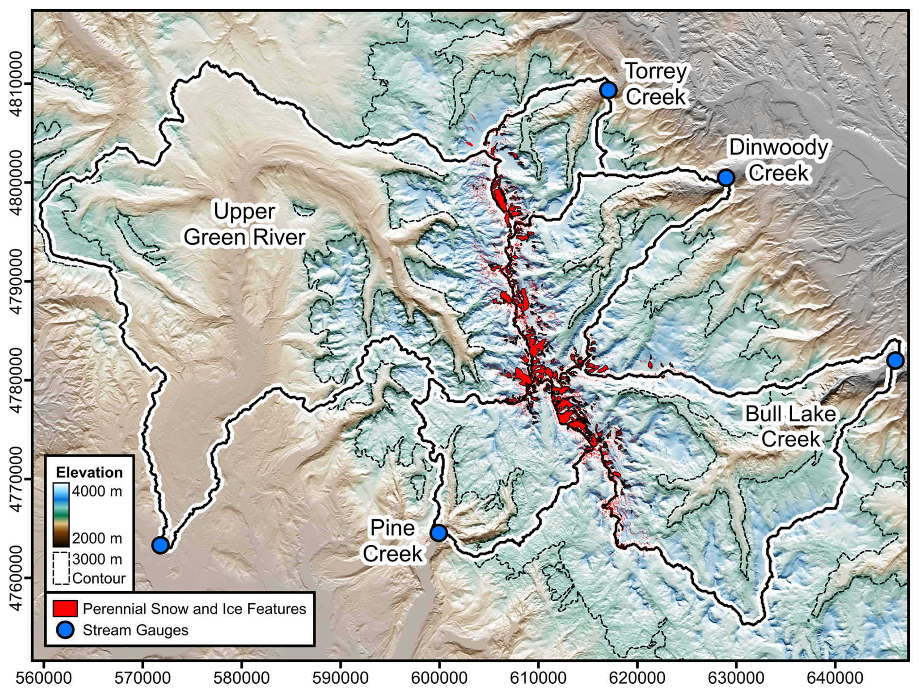
Figure 1 Relief map of the northern Wind River Range showing perennial snow and ice features considered in this study, watershed boundaries, and stream gauge locations.

Glaciological research in the WRR began nearly a century ago (Wentworth and Delo, 1931), with many subsequent studies mapping glacier areas (e.g., Meier, 1951; Thompson et al., 2011; Maloof et al., 2014; DeVisser and Fountain, 2015; Marks et al., 2015) and several studies measuring thinning rates (e.g., Marston et al., 1991; Naftz and Smith, 1993; VanLooy et al., 2013). The WRR glaciers have been generally in retreat since the Little Ice Age maximum around 1900 (Meier, 1951), with about a 44 % reduction in area since that time (DeVisser and Fountain, 2015). Climate warming is contributing to PSI mass loss, with alpine areas of the WRR warming by 3.5 °C between the mid-1960s and early 1990s based on ice core measurements (Naftz et al., 2002). Based on aerial photogrammetry and ice-penetrating radar, Marston et al. (1991) suggested that one of the WRR's largest glaciers (Dinwoody Glacier) could vanish by 2016 if mass loss continued at the 1958–1983 rate. However, the Dinwoody Glacier only decreased in area by 12 % between 1989 and 2009 (DeVisser and Fountain, 2015), highlighting the uncertainty and potential nonstationarity of mountain glacier recession rates. More recent ice-penetrating radar measurements of the Continental Glacier by VanLooy et al. (2014) suggest that at least some of its ice mass will likely persist several hundred years if the 1966–2012 thinning rate remains constant.

PSI mass loss contributes to WRR streamflow, but different approaches to quantifying this contribution on different time periods provide variable results (e.g., Marston et al., 1989; DeVisser and Fountain, 2015). Watersheds with greater PSI abundance exhibit elevated late-summer streamflow, but not all of the difference in streamflow generation among watersheds is a result of net mass loss (Bell et al., 2012). Studies based on area–volume scaling relationships tend to estimate that PSI mass loss contributes roughly 1 %–10 % of the August–September streamflow volume, and no higher than 23 % (Cheesbrough et al., 2009; Thompson et al., 2011; Maloof et al., 2014; DeVisser and Fountain, 2015; Marks et al., 2015). Studies based on stable isotope unmixing tend to provide higher estimates, e.g., 53 %–70 % of August streamflow in the most glaciated watershed and 37 %–83 % of August streamflow for two less glaciated watersheds (Cable et al., 2011; Vandeberg and VanLooy, 2016; VanLooy and Vandeberg, 2019, 2024). Measurements of surface runoff from glaciers indicate a 14 %–33 % contribution to August streamflow in two watersheds (Vandeberg and VanLooy, 2016; VanLooy and Vandeberg, 2019). Moreover, most estimates of PSI mass loss are too small to explain observed differences in late-summer streamflow among WRR watersheds with different PSI area fractions (Bell et al., 2012), provoking the question of what underlying processes might drive inter-watershed differences in both PSI abundance and late-summer streamflow.

Inter-watershed patterns of glaciation in the WRR are consistent with expected patterns of deep snow accumulation inferred from avalanches and wind transport across topographic divides (Baker, 1946). The geomorphology of the WRR is characterized by so-called “biscuit-board” topography (Hobbs, 1912), with cirques incised into high-elevation plateaus (Westgate and Branson, 1913; Blackwelder, 1915; Mears, 1993; Anderson, 2002). On these high-elevation, relatively smooth erosional surfaces, snowfall is transported downwind, accumulating in cirque basins (Graf, 1976) and sustaining PSI features at elevations below the regional ELA, similarly to “drift glaciers” observed in the Colorado Front Range (Outcalt and MacPhail, 1965; Meierding, 1982; Hoffman et al., 2007). Due to topographic shading and shelter from the prevailing wind, north-facing and east-facing aspects support more abundant and larger PSI features (Fig. 7 of DeVisser and Fountain, 2015), contributing to greater PSI abundance in watersheds on the east (downwind) side of the WRR.

3 Methods

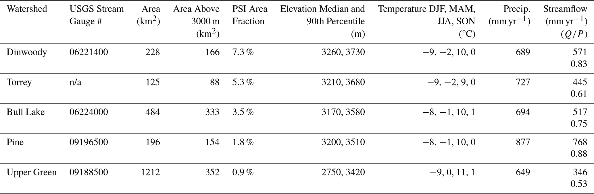
Our study leverages a combination of remote sensing, field measurements, and streamflow time series to investigate controls on the interrelationship between perennial snow and ice (PSI), seasonal snow, and water availability (Fig. 2). We further consider topographic metrics related to wind drifting and the energy balance (elevation/temperature and solar shading) to explore variability among different PSI features and watersheds. We estimate snow and ice mass changes in five adjacent WRR watersheds with repeated airborne lidar surveys. Using the geodetic method (e.g., Fischer, 2011), we map PSI mass changes by comparing lidar elevation models acquired in 2019 and 2023 with density assumptions based on literature and regional field measurements. We also use lidar to map seasonal snow accumulation near the time of peak snow water equivalent (SWE) in 2024 with snow density constrained by a statistical model based on regional field measurements. Streamflow is measured at five gauges (Fig. 1, Table 1). The watershed-average statistics in Table 1 reflect the arbitrary location of each stream gauge relative to its headwaters since gauges that are farther downstream have much larger watershed areas without meaningfully increased streamflow. We control for this effect in subsequent analysis of watershed-scale snow metrics by only considering the area above 3000 m, which approximates the snow line at the time of the 2024 lidar survey.

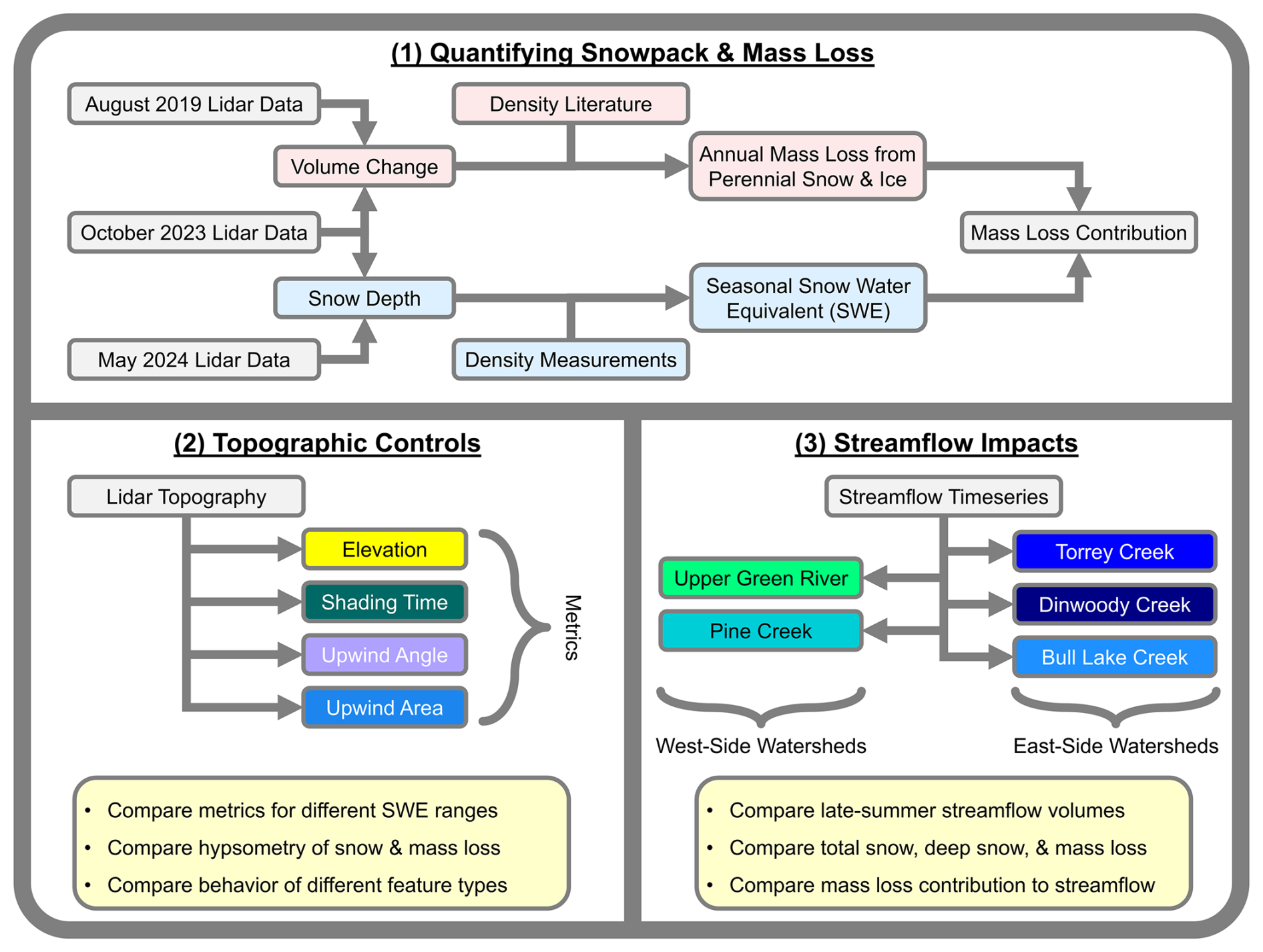
Figure 2 Methodological flowchart for this study. In part 1, we compare elevation differences across three lidar surveys and constrain densities to estimate the mass of the seasonal snowpack and annual net mass loss from perennial snow and ice. In part 2, we compare topographic metrics to evaluate controls on ablation (elevation/temperature and shading) and wind drifted snow accumulation (upwind angle and upwind area). In part 3, we evaluate the relationships between seasonal snow, net mass loss, and streamflow across five watersheds spanning both sides of the Continental Divide.

Table 1 Geographic and climatological metrics for the five gauged study watersheds arranged in order of decreasing perennial snow and ice (PSI) area fraction. DJF: December, January, and February; MAM: March, April, and May, JJA: June, July, and August; SON: September, October, and November; $Q/P$: streamflow$/$precipitation; N$/$A: not applicable. Climate data are the gridMET 1991–2020 mean (Abatzoglou, 2013). Streamflow is the 2005–2024 mean (U.S. Geological Survey, 2024a). Note that n/a stands for not applicable.

3.1 Lidar surveys

We compare digital elevation models derived from airborne lidar surveys near the end of the ablation season to estimate PSI volume changes across multiple years. The US Geological Survey (USGS) 3DEP program acquired lidar data at 1 m grid resolution over the northern Wind River Range PSI study area on 17 and 18 August 2019 (U.S. Geological Survey, 2019). Airborne Snow Observatories (ASO) acquired lidar data at 3 m grid resolution over the same area on 7 October 2023, which also includes color aerial photography at equal resolution (Painter et al., 2016). The difference in snow and ice storage between these two lidar acquisitions defines our measure of PSI net change, and areas with elevation changes between the lidar acquisitions define our concept of the active PSI area throughout this study.

Lidar datasets are reconciled and differenced to estimate elevation changes and aggregated spatially to calculate volume changes. Coregistration is necessary to minimize errors from grid mismatch. We follow the approach of Nuth and Kääb (2011) considering both horizontal shifts and an elevation-dependent bias. Our application takes advantage of parallel computing to simultaneously solve for the horizontal shift and elevation-dependent bias using numerical optimization (optimParallel library, Gerber and Furrer, 2019). We reproject and bilinearly resample the USGS 1 m digital terrain model (DTM) to match the ASO DTM. To define the control areas for coregistration, we delineate 51 landscape areas (10.6 km² total) with minimal snow or vegetation cover based on the ASO aerial photography. The coregistration areas span an elevation range of 2760 to 4120 m (median 3170 m), a slope range of 0 to 81° (median 22°), and all aspects. The numerical optimization reduces the mean absolute vertical error to 14 cm between the two DTMs, with a median elevation difference of 0.0 cm and an interquartile range of −6.3 to +8.9 cm. Steeper slopes tend to have higher errors (Pearson correlation r=0.39 between slope and absolute error), and the mean absolute error increases to 24 cm for slopes >30° (31 % of coregistration area).

We calculate the 2019–2023 DTM difference over the full survey area and then use a multi-step approach to identify changes that are likely associated with snow and ice. The USGS lidar data are classified by the lidar vendor using proprietary software based partially on lidar return intensity (Woolpert, 2020). Using this classification, we include elevation changes within all areas classified as snow-covered in the August 2019 data with the exception of frozen lakes, which are manually excluded. Bare glacier ice, rock glaciers, and buried ice features are not adequately captured by the lidar snow classification, requiring manual delineation of additional areas that exhibit spatially coherent patterns of elevation change, as demonstrated by Robson et al. (2022). We find that a ±25 cm elevation change threshold helps refine the edges of manually delineated polygons to more closely match the boundaries of apparent PSI features. All PSI features identified from elevation changes are compared with aerial imagery from Google Earth and the 2023 ASO acquisition to evaluate the likelihood of PSI occurrence in that location. In particular, we are careful to exclude steep rock features such as cliffs and sharp ridges, which cause spurious elevation differences due to lidar sampling uncertainty and slight grid mismatch.

Airborne lidar is similarly applied to map seasonal snow depths relative to the updated elevation datum from the previous year's ablation season. In this study, we map seasonal snow depth at 3 m resolution using lidar data collected by ASO on 31 May 2024. Snow depth is calculated relative to the updated 7 October 2023 PSI surfaces, and the identification of snow-covered areas is aided by imaging spectroscopy (Painter et al., 2016). Regional field measurements of snow temperature around the time of the lidar survey show a snowpack ripening elevation (0° snow temperature) around 3300 m, below 99 % of the PSI area. The following week, we observed an increase in air temperatures with no additional snow accumulation. Thus, the 2024 snow lidar survey represents approximately peak SWE conditions at PSI elevations.

The repeat lidar surveys largely cover the study watersheds. A few small PSI features (0.01–0.03 km²) representing no more than 0.5 % of the PSI area in any watershed are outside the extent of the 2023 lidar survey. Also, a portion of the Upper Green River watershed extends outside the extent of the 2024 snow lidar survey (Fig. S1 in the Supplement). We impute SWE depths at 3 m resolution for this area with a deep neural network trained on the lidar-based SWE map based on topographic metrics and Landsat fractional snow cover (U.S. Geological Survey, 2024b); details are included in Appendix B. On the test set, the imputation model achieves an R² of 0.68 for 3 m resolution SWE with an approximately unbiased mean (−0.08 cm) and median (+2.5 cm). We only use the imputed SWE values to estimate snow storage metrics in the Upper Green River watershed, thus enabling comparisons with other gauged watersheds. All PSI features considered in this study are within the lidar survey domain, and all supraglacial snow depths are directly measured by lidar.

3.2 Density constraints

Although lidar data provide useful information on spatial variability in the snowpack and PSI elevation change, we must also account for density variations to infer the spatial distribution of water mass. Relative variations in snowpack density are typically an order of magnitude smaller than variations in snow depth, but it is still important to constrain density variations across the landscape (Alford, 1967; Bormann et al., 2013; Wetlaufer et al., 2016). Density variations are especially important for deep drifts, where wind slab formation and metamorphism increase density (Tabler, 1980; Colbeck, 1982; de Leeuw et al., 2023).

We constrain snow density variations with field data from nearby regions of the WRR spanning gradients of elevation, topography, and forest canopy cover. Vertically integrated bulk snow density data are available from 20 snow pit profiles across the 6 d before the lidar survey to 1 d afterward (25 May to 1 June 2024). We also consider eight snow pit profiles from the prior year at the same point in the season (30 and 31 May 2023). Locations with repeat measurements in 2023 and 2024 show consistent densities (0 %–7 % difference) where the snow is isothermal. Thus, we include five of the 2023 measurements in our 2024 density model since those pit locations are below the snowpack ripening elevation in both years. The deepest snow pit (from 2023) extends to 485 cm depth without reaching the ground; the density profile for this pit is approximately uniform with depth (0.57 g cm⁻³ mean), so we extrapolate the mean density to the full depth of ∼ 580 cm indicated by lidar. Of the 25 total snow pits used to constrain density, 14 are above treeline, and the other 11 span a range of forest canopy cover from near 0 % to 99 % (RCMAP data: Rigge et al., 2021). We additionally include 14 snow density measurements from 5 snow telemetry (SNOTEL) sites during the same survey period, excluding days with apparent snow bridging or similar anomalies (Natural Resource Conservation Service and National Water and Climate Center, 2024).

The highest snow densities are measured in deep wind drifts, with relatively lower densities at higher elevations and generally lower (and more variable) densities under forest canopies. We did not detect an aspect dependence for density during our May–June snow surveys. We test a variety of empirical model structures, ultimately finding that a simple parametric equation is best-suited to extrapolate snow density in the study area (Appendix A, Eqs. A1–A4). Machine learning approaches such as random forest or Gaussian process regression introduce unphysical irregularities in the density field as a result of over-fitting our small sample size (N=39). Additionally, a parametric model structure allows us to include process knowledge, such as the snowpack ripening elevation and monotonically increasing bulk density in areas with greater snow depth (when all other variables are equal). Residuals from partial regression plots suggest a linear relationship between snow density and depth, a sigmoid relationship with elevation as a result of the snowpack ripening elevation, and an inverted hyperbolic relationship with forest canopy cover (small changes in canopy cover are the most important close to zero).

We use Bayesian sampling of our empirical model to extrapolate measured snow densities across the landscape (Appendix A, Eq. A5). We sample likely model parameters using the Hamiltonian Monte Carlo algorithm implemented in Stan (Stan Development Team, 2023) with error weights based on an importance score for each density measurement. The importance score is calculated by determining how often each density measurement is the closest match to the normalized predictors (depth, elevation, and canopy cover) of 10⁶ grid cells randomly sampled from the lidar survey domain with a probability equal to the grid cell snow depth. This weighted model fitting strategy has the effect of reducing uncertainty in total SWE by preferentially fitting the model to density measurements that are representative of spatially extensive and/or locally deep areas of the snowpack. Across all 39 snow density measurements, the model achieves a root mean square error (RMSE) of 0.031 g cm⁻³, which is a 7 % error relative to the 0.43 g cm⁻³ mean across measurements (Fig. S3 in the Supplement). Considering that 25 of the 39 measurements are from forested areas with similar bulk densities and a low total sum of squares (low variance), the model R² for all 39 measurements is only 0.58. However, considering just the 14 measurements above treeline or just the 12 measurements with at least 1 m of snow depth, the model R² increases to 0.93 or 0.85, respectively. The fitted model indicates a maximum rate of density change with respect to elevation at 3320 m, consistent with regional observations of the snowpack ripening elevation (∼ 3300 m based on snow temperature). We map snow density using the mean of 100 Bayesian samples for each 3 m grid cell clipped to a range of 0.30–0.60 g cm⁻³ (Fig. S4 in the Supplement).

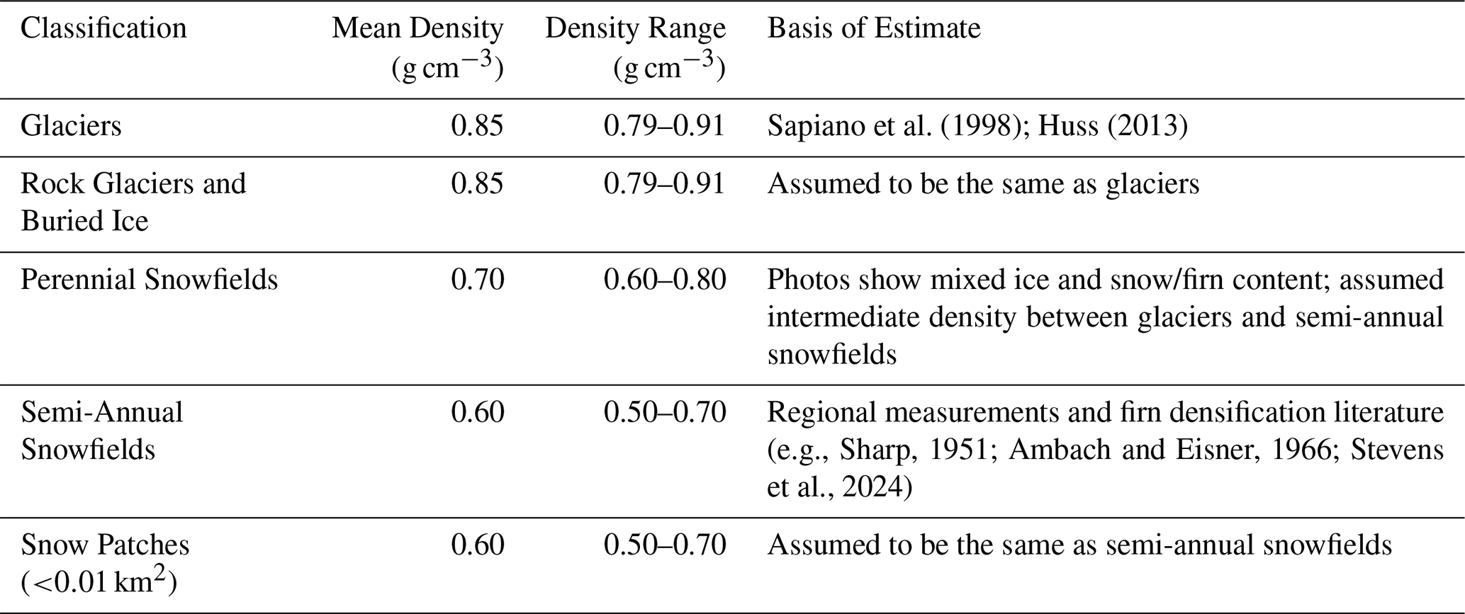
We assume a range of constant densities to convert the lidar-based 2019–2023 PSI volume change into mass (Table 2) based on our classification of PSI features (Sect. 3.3). For glaciers, rock glaciers, and buried ice, we adopt the value of 0.85 g cm⁻³ with an uncertainty range of ±0.06 g cm⁻³ (Sapiano et al., 1998; Huss, 2013). Although the volume of rock glaciers includes ice and rock, the rock volume is conserved, so we assume that elevation changes represent an equivalent depth of ice ablation. We assume that snowfields have a lower density than glaciers. One late-summer snow density measurement from 20 August 2022, indicates a bulk density of 0.58 g cm⁻³ for a semi-annual snowfield at 3480 m elevation. Based on this measurement and the range of literature values for shallow firn (e.g., Sharp, 1951; Ambach and Eisner, 1966; Stevens et al., 2024), we assume a density of 0.60 g cm⁻³ for semi-annual snowfields and 0.70 g cm⁻³ for perennial snowfields, both with an uncertainty of ±0.10 g cm⁻³. The assumption of a uniform density within each glacier or snowfield may impact spatial patterns of mass loss at the 3 m grid scale, but we expect that comparisons among PSI features and watersheds should be more robust to this assumption due to the spatial averaging of accumulation and ablation-zone density variations (Sapiano et al., 1998).

Table 2 Density assumptions for converting geodetic volume measurements into perennial snow and ice mass loss estimates.

3.3 Mass loss and SWE metrics

Returning to the methodological outline of our study (Fig. 2), we use the lidar-derived elevation changes and density constraints outlined previously to compare the seasonal snowpack with the inferred annual net mass loss from various PSI features. We also classify these features according to their morphology and behavior in order to better understand how different types of PSI relate to topography and streamflow.

Net mass loss from PSI is assumed to occur mostly in the late summer in the WRR (e.g., DeVisser and Fountain, 2015). Satellite imagery and field experience both suggest that seasonal snow usually covers most of the PSI area through July. Mean daily air temperatures (Abatzoglou, 2013) at PSI elevations drop below freezing between September (mean 3.8 °C) and October (mean −2.3 °C), which ends the ablation season. Although the 17–18 August 2019 and 7 October 2023 lidar surveys are separated by ∼ 4.1 years, we assume that the difference between these two surveys represents 4.5 years of ablation because the 2019 data are about halfway through the presumed ablation season and the 2023 data represent late-season conditions. Variations in the persistence of the seasonal snowpack and differences in the timing of lidar surveys both contribute uncertainty to our estimates of the PSI mass loss rate, but we constrain this uncertainty based on the 2024 snow data (Sect. 2.4).

To estimate the potential impact of deglaciation on streamflow, we define the “mass loss contribution” as the fraction of total annual meltwater derived from net mass loss. A PSI feature with a zero or positive mass balance would have a mass loss contribution of zero since its meltwater would be entirely derived from seasonal snow and sustainable ice flow. We estimate the mass loss contribution for each PSI feature by dividing its annual mass loss by the sum of mass loss and seasonal snow mass. We emphasize that this metric is primarily intended for inter-feature comparisons of meltwater sustainability and is not a definite measure of the PSI surface mass balance.

We aggregate seasonal snow and annual mass loss statistics within the boundaries of discrete PSI features, with each feature >0.01 km² classified as a glacier (if crevasses are present indicating movement), perennial snowfield, rock glacier, buried ice, or semi-annual snowfield (Fig. 3). Glaciers and rock glaciers flow, while perennial snowfields are static. The buried ice category includes debris-mantled glacier margins and ice-cored moraine remnants (Fig. S6 in the Supplement), some of which show morphological indications of movement though they lack a steep headwall rockfall source and are not rock glaciers. We define a new category of “semi-annual snowfields” that exhibit net mass loss between 2019 and 2023 but which are not identified as PSI >0.01 km² in the 2015 imagery used by Fountain et al. (2023). Some of these semi-annual features are present in both the 2019 and 2023 lidar data, while others appear to have melted completely over that time. The numerous remaining features that are too small for manual classification are grouped together as “small snow patches”, varying in size from the grid scale (9 m²) to roughly 0.01 km².

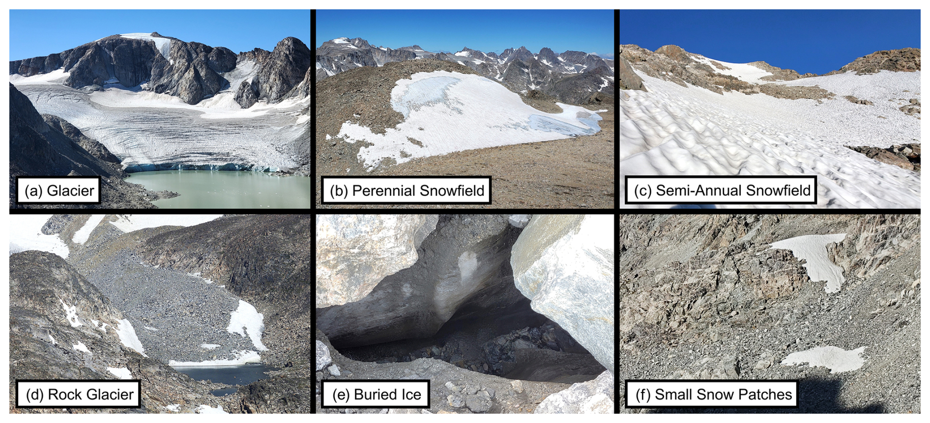
Figure 3 Photos from the WRR study area showing examples of a glacier (a), a perennial snowfield (b), semi-annual snowfield (c), rock glacier (d), buried ice (e), and small snow patches (f).

We identify glacier and perennial snowfield boundaries primarily from polygons delineated manually by Fountain et al. (2022, 2023). Due to the challenges of identifying buried ice and active rock glaciers from aerial imagery, we supplement this dataset with additional features identified from spatially coherent patterns of elevation change (Sect. 2.1). We acknowledge that our elevation-based approach only identifies areas of buried ice and rock glaciers that are actively melting, but we are primarily interested in identifying PSI features that are contributing net mass loss to streamflow. Several apparent fossil rock glaciers that do not show coherent elevation change are excluded from our analysis. We note that some rock glaciers and buried ice features also have a surface snow expression and that the separation of these categories from connected glaciers or snowfields is not definitive (Anderson et al., 2018). We follow the criteria of Fountain et al. (2023) to separate rock glaciers and fore-field connected glaciers based on the presence of an intervening topographic depression. Classification of PSI features among the various categories is also aided by opportunistic photos curated from numerous recreational mountaineering trips in the study area between 2015 and 2024 (e.g., Fig. 3).

Hereafter, we use the generic term “perennial snow and ice” (PSI) to refer to the entire population of six feature types identified in Fig. 3. Similarly, the generic term “net mass loss” refers to 2019–2023 mass loss from the entire population of all six feature types. In certain figures, tables, and other results, we restrict our analysis to specific types of PSI features; these specific subsets are explicitly identified wherever they appear.

3.4 Mass loss uncertainty

Seasonal snow variations contribute potential uncertainty to the 2019–2023 estimate of PSI mass loss. The 2019 USGS lidar data were collected on 17–18 August, about a month before the typical end of the ablation season. The lidar intensity shows bare ice below 3500–3600 m on the large glaciers, consistent with late ablation season conditions. However, some snowfields are larger than their minimum extent observed in prior 2015 imagery (Fountain et al., 2023), suggesting that some seasonal snow may remain in the 2019 lidar data. The 2023 lidar survey was acquired after an early October snowfall, but coincident fieldwork indicates that snow depths were on the same order of magnitude as the ground roughness (∼ 5–15 cm at 3800 m, above the median PSI elevation of 3650 m). Due to the small (14 cm) coregistration error between surveys, we expect the largest source of uncertainty in the mass loss rate to derive from potential differences in the amount of snow present between late August of 2019 and early October of 2023. We derive a conservative upper bound for this uncertainty based on the 2024 SWE data, assuming that no more than 10 % of the seasonal snowpack remains at the time of the ablation-season lidar acquisitions. The assumption that >90 % of snowmelt occurs by late August is supported by streamflow timing since September–October streamflow represents only 9.3 % of the average May–October volume across the five study watersheds. Thus, regardless of whether there was more snow in August 2019 (remaining from the previous winter) or more snow in October 2023 (accumulated in the prior week), uncertainty introduced by seasonal snow variability should not exceed 10 % of the total seasonal snowpack. We evaluate the sensitivity of our watershed mass loss estimates to this plausible range of snow variability by adding ±10 % of the 2024 SWE depth to each PSI grid cell.

We combine uncertainty arising from seasonal snow variability and PSI density estimates to derive a final PSI mass loss uncertainty. Assuming the two uncertainty sources are independent, we combine the relative uncertainty from seasonal snow (±10 % of the 2024 SWE) and the assumed PSI density ranges (±0.06 or ±0.10 g cm⁻³; Table 2) for each grid cell. The lower bound on mass loss is derived from the lower density with 10 % of the 2024 SWE subtracted from the mass loss, while the upper bound on the mass loss rate is derived from the higher density with 10 % of the 2024 SWE added to the mass loss.

3.5 Topographic indices

Returning to our methodological overview in Fig. 2, we now consider topographic controls on spatial variability in snow accumulation and PSI mass loss. We define four topographic metrics related to snow accumulation and the energy available for melt: elevation, solar shading, upwind angle, and upwind area (Fig. 4). Elevation is a proxy for air temperature, assuming that temperature lapse rates are consistent over the relatively small PSI study area (∼ 400 km² bounding convex hull). We calculate mean ablation-season (July–September) sun exposure time at 30 m resolution (WhiteboxTools library, Lindsay, 2016) to account for the effect of terrain shading on solar insolation, which is the most influential factor controlling energy balance heterogeneity across a glacier (Wolken, 2000; Oerlemans and Klok, 2002). Shading time is a coarse energy balance metric that does not capture the variable effects of cloudiness and seasonality (Olyphant, 1984) or longwave radiation from rock walls (Olyphant, 1986). Nevertheless, we expect topographic shading to positively correlate with snow persistence and reduce the PSI ablation rate (e.g., Williams et al., 1972; Munro and Young, 1982; Delmas et al., 2014; Olson and Rupper, 2019; Florentine et al., 2020).

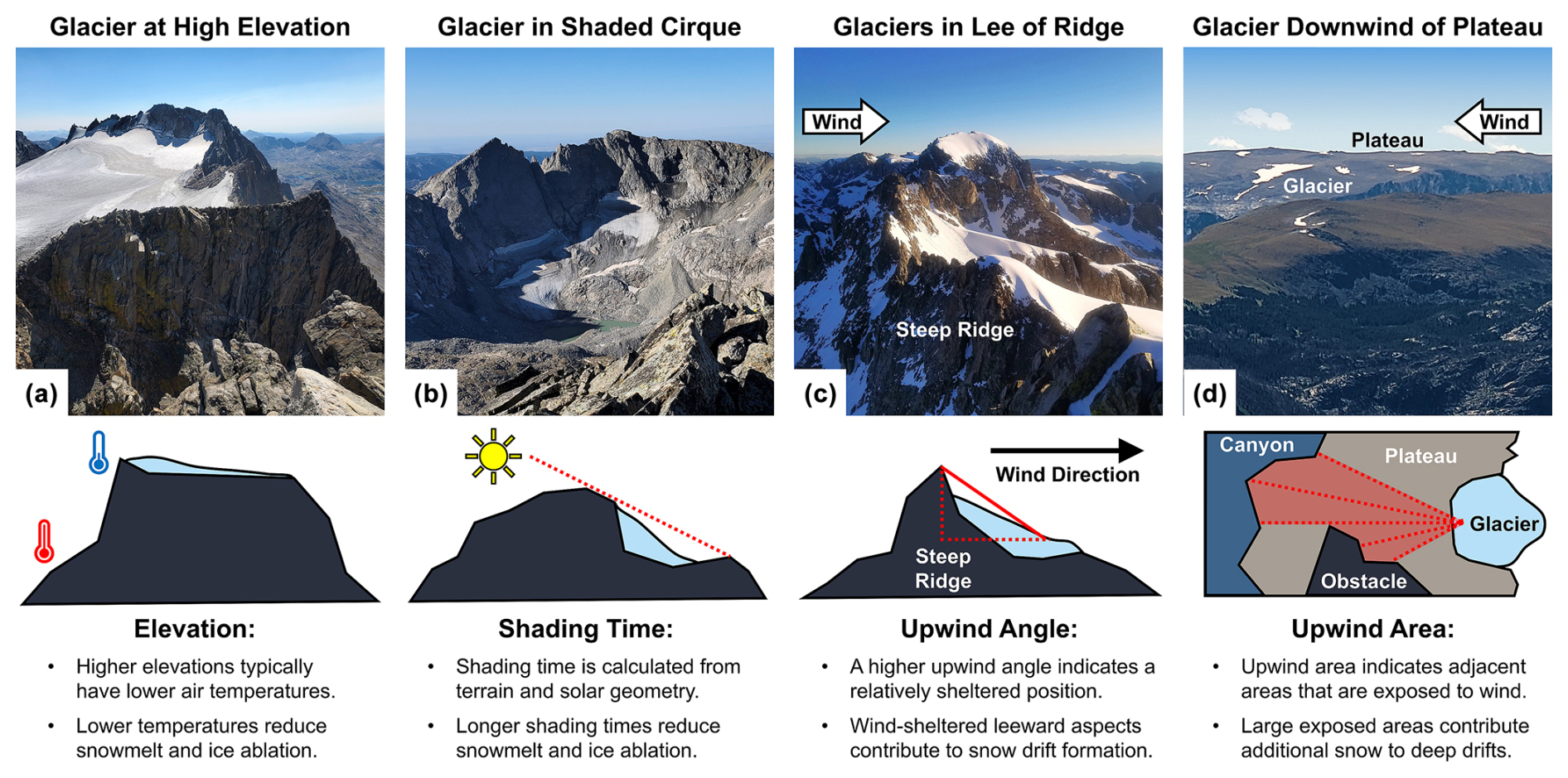
Figure 4 Example photos and conceptual models of the four topographic indices for the glaciers shown in Fig. 8. The Upper Fremont Glacier (a) is notable for its high elevation; the Stroud Glacier (b) is notable for its shaded position in a north-facing cirque; the Gooseneck and Dinwoody glaciers (c) are notable for their position on the downwind side of a steep ridge, which provides wind shelter; and the glacier on Dry Creek Ridge (d) is notable for the exposed plateau on its upwind side that provides a large snow drift source area.

Topographic wind drift indices are also useful for investigating spatial patterns of snow accumulation and glaciation in mountain environments (e.g., Lapen and Martz, 1993; Purves et al., 1999; Winstral and Marks, 2002; Anderton et al., 2004; Freudiger et al., 2017). We calculate the maximum horizon angle in the upwind direction (hereafter the “upwind angle”), which is the Sx parameter defined by Winstral et al. (2002). Grid cells with a positive upwind angle are sheltered from the wind by terrain obstacles, which promotes drift formation, and a steeper upwind angle indicates a more sheltered location. Calculating the upwind angle requires defining a prevailing wind direction, which is approximately west to east based on anecdotal observations, continuous measurements by an automatic weather station in the Torrey Creek watershed (operated on ranch land by the authors), and NLDAS-2 climatology (Fig. S2 in the Supplement; Xia et al., 2012). We calculate the upwind angle from a digital elevation model (Farr et al., 2007) at 30 m resolution with an unlimited upwind search distance. Additionally, we calculate the same index using the 3 m lidar DTM with a maximum search distance of 100 m to capture small-scale terrain effects. We combine both resolutions by interpolating the coarser raster to 3 m and taking the maximum upwind angle from short- and long-distance calculations. Since wind varies between storms and is deflected by mountainous terrain, we average the upwind angle over an azimuth range from 240° to 300° in 1° increments to account for a range of plausible shelter and scour configurations.

A new topographic wind index, the upwind area, can highlight likely drift accumulation areas on the downwind margins of high-elevation plateaus, which are a notable feature of the WRR (Anderson, 2002). Although the upwind angle is useful for explaining drift locations within small watersheds (e.g., Winstral et al., 2002), it does not account for variations in the size of contributing source areas, which is an important control on deep drift formation (Outcalt and MacPhail, 1965). Elevated plateau surfaces in the northern WRR are conducive to long-distance snow transport, leading to deep drifts in downwind topographic depressions. Some of the drifting snow from these plateaus collects in cirque basins, but large drifts can also form in relatively shallow depressions where the upwind angle index does not predict drift formation (e.g., Figs. 4d and 8d). To better capture WRR drift patterns, we estimate the upwind area, a two-dimensional index based on the extent of upwind areas that are exposed to the wind and a downwind distance factor accounting for deposition and avalanches from steep cliffs (Appendix C, Eqs. C1–C9). The upwind area index only considers potential contributing areas that are not separated from the local grid cell by large intervening sheltered areas since terrain obstacles can interrupt wind transport (Fig. 4d).

To relate heterogeneity in PSI accumulation and ablation to wind drifting and energy inputs, we develop a classification based on the four topographic indices (elevation, shading time, upwind angle, and upwind area). The topographic indices are linearly rescaled within the interquartile range of topographic variability across all PSI grid cells. This approach to normalization preserves heavy distribution tails, which helps identify cells dominated by a given index. For grid cells with at least one topographic index exceeding the upper quartile of that index for all PSI cells, the index with the largest rescaled value is assigned as the dominant classification. Aggregating SWE and mass loss rates within cells dominated by a given topographic index provides a measure of each index's relationship to accumulation and ablation patterns. To evaluate the relationship between wind drifting and seasonal snow at the watershed scale, we also classify snow-covered grid cells that exceed the median value of the upwind angle and/or upwind area indices within the full snow-covered area. We then aggregate SWE in areas with and without an above-median wind drift index using different minimum SWE thresholds.

3.6 Controls on streamflow

Constraining the streamflow contribution from unsustainable meltwater (PSI net mass loss) is one of the key goals of the present study (Fig. 2). To explore mass loss contributions to the downstream water supply, we compare watershed-average annual PSI mass loss with late-summer streamflow averaged over the study period. US Geological Survey (USGS) stream gauges each provide continuous daily flow records for four of the study watersheds (Table 1; U.S. Geological Survey, 2024a), and the Torrey Creek stream gauge is operated by the authors. We aggregate yearly, August–September, and July–September mean streamflow for all five gauges over water years 2020–2023 to compare with PSI mass loss between the 2019 and 2023 lidar surveys. Assuming that evapotranspiration is energy-limited (but not necessarily zero) along the downstream flow paths from PSI areas as a result of ecosystem adaptation to perennial water availability (e.g., Gentine et al., 2012), we can directly estimate the contribution of mass loss to streamflow since an additional volume of PSI melt would contribute an equal volume of additional streamflow. An energy-limited assumption for the PSI contribution to evapotranspiration is reasonable because meltwater from most PSI features immediately forms perennial streams, demonstrating that the available water exceeds potential evapotranspiration along the downstream flow paths.

The Torrey Creek stream gauge is newly operated beginning in water year 2022, so we estimate prior streamflow records through machine learning imputation. We impute Torrey Creek streamflow prior to 2022 using Gaussian process regression (DiceKriging library, Roustant et al., 2012) based on the four other gauges and a seasonal sine wave. We test the validity of this imputation by predicting 2024 Torrey Creek streamflow from only the 2022–2023 data, which yields a daily Nash–Sutcliffe efficiency of 0.93 and a bias of 2 %. We then use all available Torrey Creek data (water years 2022–2024) to impute the 2005–2021 period, which moderates the effect of discrete storm events on the annual hydrograph for visualization and inter-watershed comparison purposes.

We test the sensitivity of historic streamflow patterns to further PSI recession by subtracting watershed-average mass loss rates from late-summer streamflow. We create daily-average hydrographs for each gauge over the past 20 water years (2005–2024) to reduce the effect of stochastic storms on our inter-watershed hydrograph shape comparisons, but we only consider water years 2020–2023 to estimate the mass loss contribution since that period matches the lidar survey timing. Normalizing each watershed's hydrograph by the mean May–September flow allows us to compare runoff timing, and normalizing specific runoff (mm d⁻¹) by the daily mean across watersheds allows us to identify watersheds that produce relatively more or less water at a given time of year. We estimate the potential impact of complete deglaciation on the downstream hydrograph by reducing each watershed's August–September streamflow in proportion to the estimated PSI mass loss fraction. This counterfactual scenario is a conservative lower bound on late-summer streamflow in the absence of PSI retreat because at least some mass loss probably occurs earlier in the summer.

To identify dominant controls on streamflow patterns, we normalize melt-season hydrographs by area-averaged snow storage metrics and identify periods where a particular metric best explains the streamflow differences between watersheds. Streamflow normalized by snowpack volume is analogous to a runoff ratio. We also normalize streamflow by the volume of water stored in areas with SWE deeper than the 75th, 90th, or 95th percentile across the five-watershed study area, corresponding to a minimum depth of 0.65, 1.26 m, or 1.72 m of SWE. These dimensionless hydrograph metrics provide a proxy for the relationship between snow persistence and streamflow production since deep snow drifts melt relatively slowly compared to the same snow spread thinly. For each day in May–September, we further normalize each of these hydrograph metrics by the mean across watersheds to identify which watersheds are over- or under-producing streamflow relative to a given snow storage metric. On a given day, we assume that inter-watershed streamflow patterns are best explained by whichever normalized hydrograph metric has the lowest root-mean-square difference between watersheds. For example, if streamflow divided by snow storage approximately equals a constant value for all watersheds at a given point in the melt season, then we conclude that inter-watershed differences in snow storage can explain inter-watershed streamflow differences for that time period.

4 Results

The 2024 SWE map (Fig. S5 in the Supplement) shows a snow-covered area of 1144 km² within the five study watersheds on 31 May (51 % of total area). The 2019–2023 elevation difference map (Fig. S7 in the Supplement) shows an area of 58 km² with elevation changes that are likely associated with snow and ice (Sect. 3.1). Over this period, 93 % of all PSI areas exhibit a decrease in elevation, and 7 % exhibit an increase.

4.1 Mass loss estimates

In order to evaluate the hydrological effects of melting PSI, we first estimate the spatial distribution of annual net mass loss. Since different types of PSI features (glaciers, snowfields, rock glaciers, etc.) may respond differently to climate, we quantify mass loss separately for each of these feature classes.

We classify a total of 338 PSI features with area >0.01 km² (including semi-annual snowfields), all of which experienced a net mass loss (Table 3). The Sourdough and Grasshopper glaciers experienced a terminal retreat of 60–120 m between 2019 and 2023, the fastest retreat of all WRR glaciers (Figs. S8–S9 in the Supplement). Conversely, some PSI features did not exhibit appreciable area change despite thinning. Although the mean surface elevation of all PSI decreased, some glaciers and snowfields exhibited small areas of elevation increase, probably from shifting snow drifts. The mean annual mass loss rate for “large” glaciers (>0.5 km²) is 27 % faster than that for “small” glaciers. Relative to the mean across all glaciers (0.99 m yr⁻¹), the mean loss rate is 30 % slower for perennial snowfields, 80 % slower for rock glaciers, and 49 % slower for buried ice.

Table 3 Mass loss rates for different PSI feature classifications. Area measurements represent the feature area in 2019. The area range is the minimum and maximum for the N features actually included in that class. The mass loss minimum, maximum, and mean are area-averaged within discrete features in that class. Values in parentheses are uncertainty bounds.

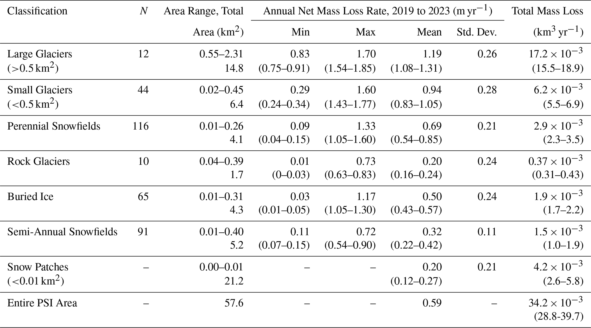
The 12 large glaciers contribute 50 % of the total mass loss despite only representing 26 % of the total PSI area. Small glaciers (11 % of PSI area) contribute 18 %, perennial snowfields (7 % of PSI area) contribute 8 %, rock glaciers (3 % of PSI area) contribute 1 %, and buried ice features (7 % of PSI area) contribute 6 %. The remaining 17 % of mass loss derives from semi-annual features (9 % of PSI area) and snow patches <0.01 km² (37 % of PSI area). Considering only features >0.01 km² and excluding the semi-annual snowfields, glaciers contribute 82 % of the mass loss, perennial snowfields 10 %, rock glaciers 1 %, and buried ice 7 %.

The manually classified glaciers, perennial snowfields, rock glaciers, and buried ice features account for 83 % of the total estimated mass loss between 17 and 18 August 2019 and 7 October 2023. The remaining fraction derives from features that are <0.01 km² at the time of the 2015 imagery used by Fountain et al. (2023). Among these features, 91 are larger than 0.01 km² in the 2019 data, indicating that they increased in area between 2015 and 2019. However, all of these features still experienced an elevation decrease between 2019 and 2023, with some vanishing completely. These “semi-annual” features contribute 5 % of the total mass loss between 2019 and 2023. Some of the semi-annual features could represent seasonal snow remaining in the August 2019 data, which illustrates how variations in seasonal snow persistence contribute to uncertainty in our annual PSI mass loss estimate (Sect. 3.4). Finally, 12 % of the total mass loss derives from snow patches that are detected by the 2019 lidar classification but <0.01 km² in all considered datasets. These snow patches are too numerous for individual classification, and they likely represent a combination of semi-annual and true perennial features.

The total PSI mass loss uncertainty is ±16 %, including uncertainty propagated from the density assumptions and potential variability in seasonal snow between the lidar survey dates. Seasonal snow variability is a smaller fraction of the measured elevation change for glaciers, which experience the largest changes (Table 3). Consequentially, mass loss from large glaciers and small glaciers is less uncertain (±10 % or ±11 %, respectively) than mass loss from buried ice (±13 %), rock glaciers (±16 %), perennial snowfields (±21 %), semi-annual snowfields (±30 %), and small snow patches (±38 %).

4.2 Seasonal snow and net mass loss relationships

We compare spatial patterns of SWE and PSI net mass loss to investigate their relative importance for determining total melt and hence the vulnerability of the downstream water supply. Enhanced snow accumulation and shading in cirque basins can reduce the mass loss contribution of PSI features in topographic refugia, with deep supraglacial snow contributing a more sustainable source of meltwater.

Figure 5 illustrates the difference between two glaciers that are endmembers of accumulation and mass loss variability in the WRR. The example small glacier (0.21 km², unnamed but ca. Ross Lake) has a 26 % slower mass loss rate compared to the example large glacier (1.47 km², Grasshopper Glacier) despite the large glacier's 300 m higher median elevation. The small glacier has a mean 2024 SWE depth of 4.0 m, which is 160 % more than the large glacier (1.5 m mean SWE). A decoupling of the mass loss rate from elevation is also observed within the perimeters of these glaciers. Lower elevations exhibit a consistently faster mass loss rate for the large glacier (Pearson correlation $r=-\mathrm{0.70}$) with the exception of a lake-terminating portion. In contrast, there is no linear relationship between elevation and mass loss rate for the small glacier ($r=-\mathrm{0.05}$). Instead, spatial variability in the small glacier's mass loss rate is positively correlated with SWE (r=0.65) unlike the large higher elevation glacier, which has a negative correlation between mass loss and SWE ($r=-\mathrm{0.41}$). The positive correlation between deeper snow and faster mass loss within the small glacier is unintuitive, and this relationship appears to indicate that the small glacier is more sensitive to annual snow accumulation rather than temperature. Reduced accumulation or reduced seasonal snow persistence in 2023 compared to 2019 likely accounts for some of the small glacier's mass loss.

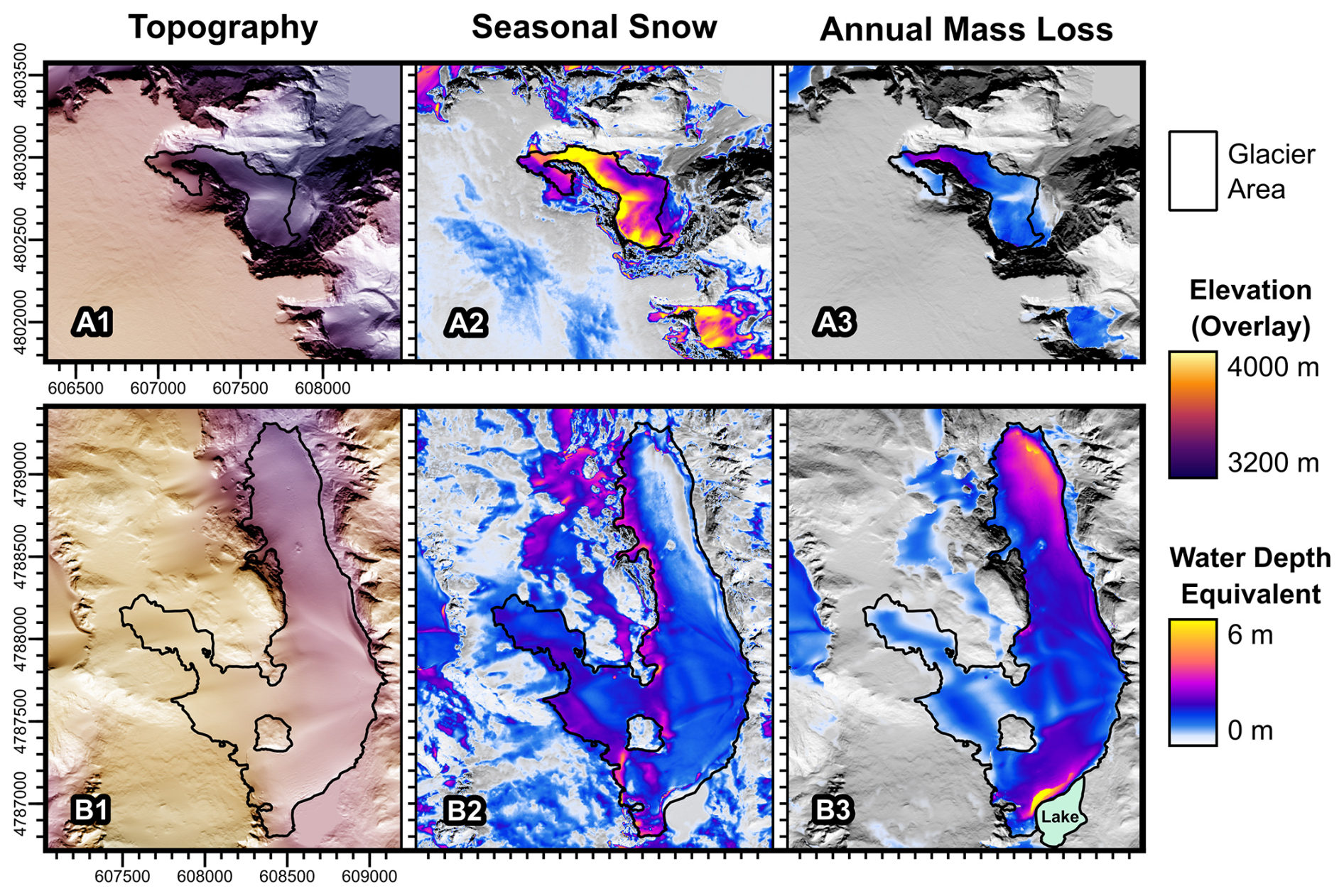
Figure 5 Comparison of 2024 seasonal snow water equivalent (SWE) and 2019–2023 annual mass loss rate for a small glacier near Ross Lake (0.21 km², a1–a3) and the large Grasshopper Glacier (1.47 km², b1–b3). Glacier perimeters and areas date to 2019. (a1) and (b1) illustrate topography with shaded relief and a color-coded elevation overlay. (a2) and (b2) illustrate seasonal snow. (a3) and (b3) illustrate annual mass loss. Seasonal snow and annual mass loss are both in units of water depth equivalent with the same color ramp. Photos of these glaciers and their terrain indices are shown in Figs. S15–S16 in the Supplement.

To investigate the balance of topographic and climatological controls on interrelationships between snow and PSI mass low, we compare the elevation hypsometry of different PSI features since elevation is assumed to be a rough proxy for temperature. We observe greater variability in the elevational distribution of snow and net mass loss among features <0.5 km² (Fig. 6 and Figs. S10–S12 in the Supplement). The deepest snow accumulation zones generally occur at relatively low elevations. By only considering snow hypsometry within the perimeters of perennial features, we selectively sample areas of deep snow accumulation. In other words, there is a survivorship bias in Fig. 6 since low-elevation PSI features are preferentially located in areas with enhanced accumulation and limited ablation, which explains the unintuitive finding that lower elevations have deeper supraglacial snow depths (Fig. S14 in the Supplement). Across full watersheds, deeper mean SWE depths are observed at relatively high elevations (Figs. S13 in the Supplement). The large glaciers (>0.5 km²) exhibit faster mass loss rates at lower elevations, consistent with the example large glacier in Fig. 5. Within the perimeters of the large glaciers, the mass loss rate has a mean correlation of −0.60 with elevation, in contrast to small glaciers, where the mean correlation is weak ($r=-\mathrm{0.16}$).

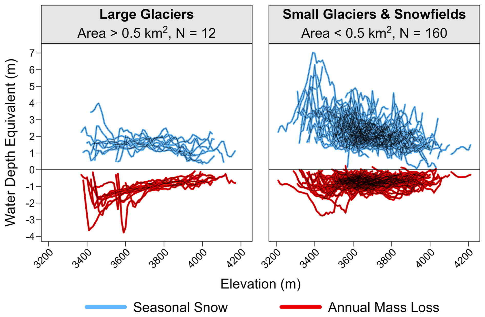
Figure 6 Elevation hypsometry of seasonal snow (2024) and annual mass loss (2019–2023) for large glaciers or small glaciers and perennial snowfields showing a wider range of variability in both accumulation and ablation for relatively small features. Example photos and individual hypsometry profiles from each of the large glaciers are shown in Figs. S10–S11 in the Supplement.

Net mass loss contributes a smaller fraction of the total meltwater generated by PSI features with relatively deep seasonal snowpacks (Fig. 7). In general, the large glaciers have relatively shallow mean SWE depths (1.0–1.8 m), with a roughly equal annual mass loss rate (0.8–1.7 m). As a result, the mass loss contribution for the 12 large glaciers varies between 36 %–53 %. The deepest snow accumulation zones sustain relatively small PSI features. For glaciers and perennial snowfields with more than 3 m of seasonal SWE (N=29, area of 0.01–0.21 km²), only 10 %–26 % of yearly meltwater derives from net mass loss. Perennial snowfields tend to have deeper seasonal SWE and a smaller mass loss contribution compared to glaciers (Fig. 7). Rock glaciers exhibit the shallowest snow accumulation (mean 1.0 m SWE). Nevertheless, rock glaciers have a mean mass loss contribution of 13 %, much smaller than the mean mass loss contribution of 31 % for glaciers and snowfields with comparable seasonal SWE <2 m. Buried ice features, including debris-mantled glacier margins, similarly have relatively low mean SWE (1.6 m), but the mean mass loss contribution from buried ice (25 %) is almost twice as high as from rock glaciers.

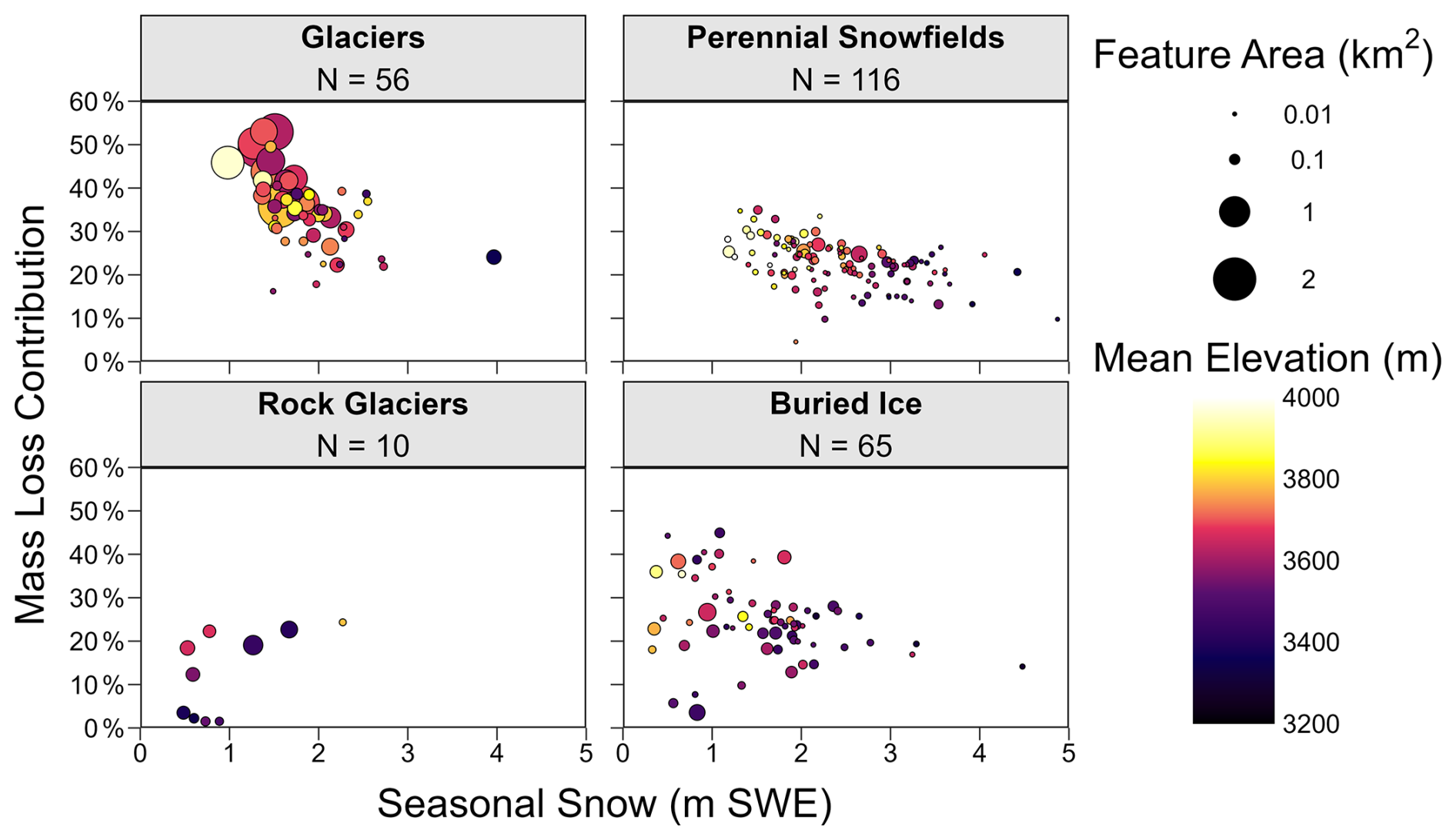
Figure 7 Approximate fraction of total meltwater (seasonal snow plus annual net mass loss) that is derived from net mass loss for 247 PSI features classified as glaciers, perennial snowfields, rock glaciers, or buried ice. Photo examples of a glacier, perennial snowfield, rock glacier, and buried ice are shown in Fig. 2.

4.3 Topographic controls

Indices related to wind drifting and energy inputs reveal topographic controls on the interrelationship between snow and mass loss. In Fig. 8, we compare terrain indices and the mass loss contribution for the same four glaciers from Fig. 4, each of which exemplify one of the four terrain indices (elevation, shading time, upwind angle, and upwind area). Maps of seasonal snow and annual mass loss for these glaciers are show in Fig. S17 in the Supplement.

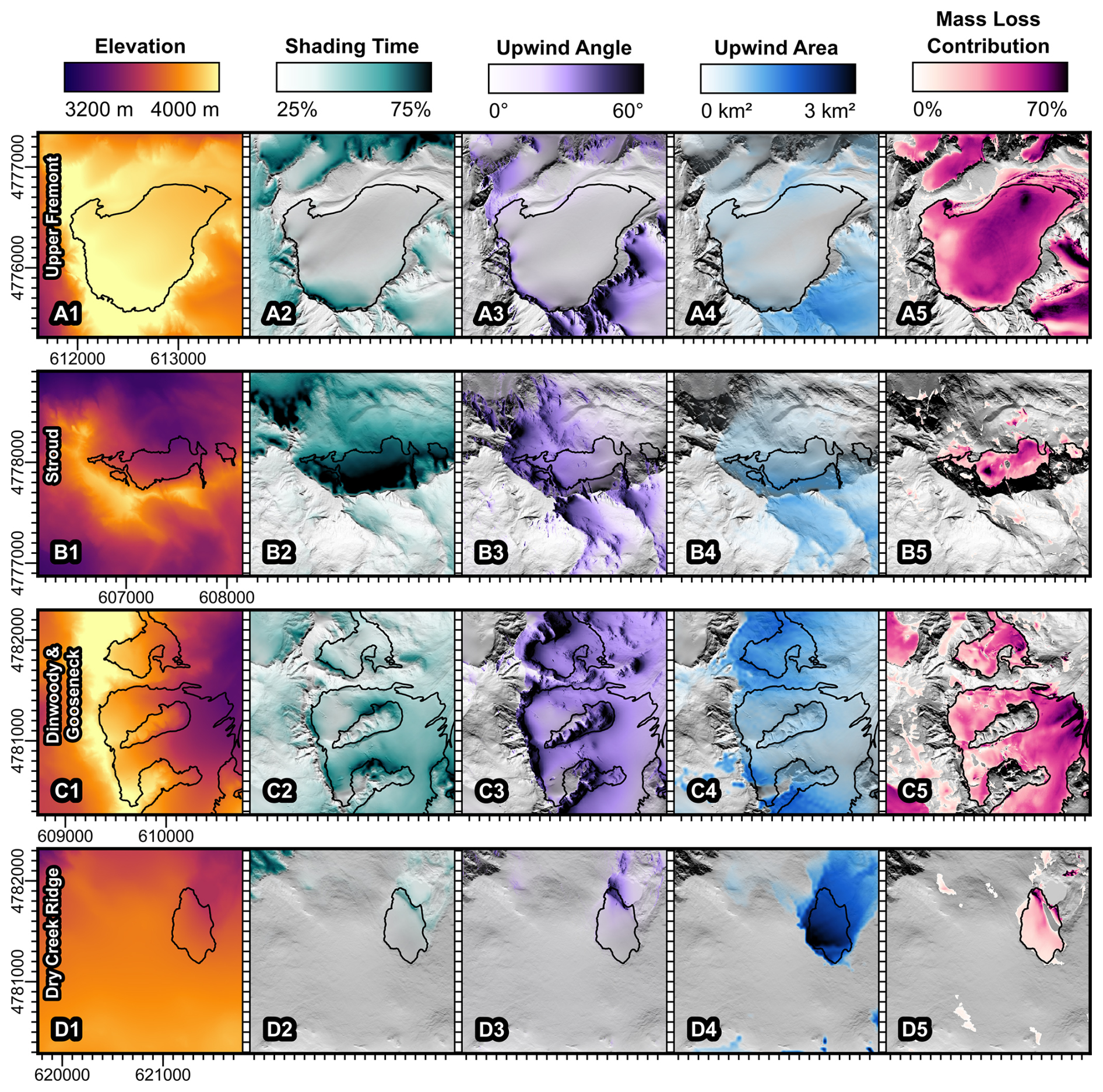
Figure 8 Maps of glaciers that exemplify each of the four terrain indices: elevation (a1–a5), shading time (b1–b5), upwind angle (c1–c5), and upwind area (d1–d5). The mass loss contribution defines the ratio of net mass loss to total ablation (seasonal snow and mass loss). All maps are on the same scale. Example photos of these glaciers and conceptual models of the terrain indices are shown in Fig. 4.

The elevation-dominated (air temperature) Upper Fremont Glacier (Fig. 8a1–a5) is characterized by a high elevation (mean 3960 m), a gentle slope (mean 11°), and the shallowest snowpack of all 12 large glaciers (mean 1.0 m). Despite its high elevation, this glacier experiences a relatively high mass loss contribution of 46 %.

By contrast, a steep north-facing cliff shelters the Stroud Glacier (Fig. 8b1–b5) from solar insolation. Despite being 400 m lower than the Upper Fremont Glacier, the Stroud Glacier is shaded for 71 % of daylight hours and spends less than half as much time exposed to the sun, limiting its mass loss contribution to 34 %.

A sharp north–south ridgeline contributes to wind drifting on top of the Gooseneck and Dinwoody glaciers (Fig. 8c1–c5), which have steep upwind angles (mean 39 and 31°) providing wind shelter. These heavily drifted glaciers have about twice as much seasonal snow (mean 2.1 and 1.8 m) as the Upper Fremont Glacier despite their 180–270 m lower mean elevation.

Although both wind indices can identify potential drift formation regions in cirque basins (Fig. S15a2–a3 in the Supplement), the upwind area index also highlights shallow depressions downwind of large plateaus. The glacier exemplifying the upwind area index (Fig. 8d1–d5, unnamed but ca. Dry Creek Ridge) has a relatively low elevation (mean 3680 m), minimal terrain shading (mean 34 % shade time), and moderate upwind angle (mean 17°), but it still has the smallest mass loss contribution (22 %) of all glacier and perennial snow features with an area >0.1 km². The upwind area index suggests that this glacier could accumulate snow from a ∼ 3 km² contributing area. As a result of shifting snow drifts, this glacier exhibits an increase in surface elevation over 8 % of its area between 2019 and 2023 despite its 0.63 m yr⁻¹ mass loss rate.

To generalize our analysis of topographic controls beyond the four glaciers considered in Fig. 8, we now consider the relative importance of each control across the entire population of PSI features. The deepest snow is almost all associated with topographic controls on wind transport (Fig. 9). Although only 8 % of all PSI grid cells have seasonal SWE > 3 m, these deep accumulation zones are important for the sustainability of PSI meltwater because deeper accumulation is associated with a lower net mass loss contribution (Fig. 7). For PSI with SWE > 3 m, 63 % of grid cells exceed the top quartile of wind drift indices (upwind angle or upwind area), and this fraction increases to 76 % for SWE > 4 m (2 % of area) and 92 % for SWE > 6 m (0.2 % of area). Large upwind-contributing areas produce the deepest drifts, and the upwind area index is the dominant control for 68 % of PSI grid cells with SWE > 6 m.

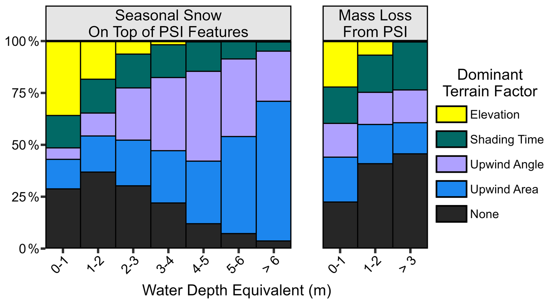
Figure 9 Relative importance of terrain-based indices for PSI grid cells across a range of 2024 seasonal snow water equivalent (SWE) depths and 2019–2023 annual net mass loss rates.

PSI features with elevation as the only dominant topographic factor (16 % of PSI area) have relatively low snow accumulation and slow mass loss rates (Fig. 9). Elevation-dominated PSI features have a mean SWE depth of 1.3 m and a mean mass loss rate of 0.47 m yr⁻¹ compared to 1.8 m and 0.59 m yr⁻¹ for all PSI features. The relatively shallow snow accumulation associated with elevation-dominated PSI features is also consistent with our finding that the deepest snow occurs at relatively low elevations (Fig. 6). There is a fairly consistent 14 %–16 % of the PSI area dominated by topographic shading for all SWE depth ranges < 5 m, but only 7 % of the PSI area is dominated by shading for SWE > 5 m.

Watersheds with favorable topography for wind drifting exhibit extensive areas of deep snow despite having less total snow accumulation (Fig. 10). Watersheds on the east side of the Continental Divide (Torrey, Dinwoody, and Bull Lake Creeks) exhibit relatively low total snow storage, with 24 % less area-normalized SWE above 3000 m relative to the west-side watersheds (Upper Green River and Pine Creek). This landscape-scale pattern of snow storage is consistent with orographic precipitation from prevailing west-to-east storm tracks and may be exaggerated by sublimation from snow blowing over the crest of the mountain range. The east-side watersheds have greater SWE depth variability, with a standard deviation of 0.63 m for SWE depths at 3 m resolution, which is 35 % higher than the west-side watersheds (standard deviation 0.47 m). The 90th and 95th percentile SWE depths are 1.37 and 1.87 m in the east-side watersheds compared to 1.19 and 1.51 m in the west-side watersheds. Consequentially, despite having less total SWE (−24 %) relative to the west-side watersheds, the east-side watersheds have about the same (−7 %) SWE deeper than 1 m and almost twice as much (+90 %) SWE deeper than 2 m.

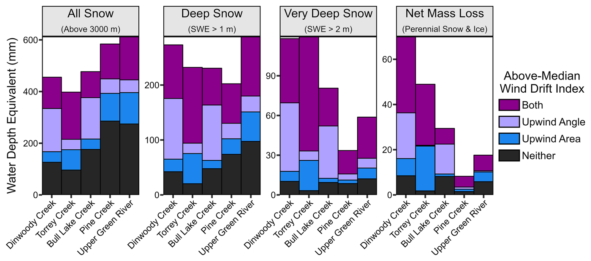
Figure 10 Area-average 2024 SWE and 2019–2023 mass loss in each watershed classified according to whether one or both of the topographic wind drift indices is above the median for the snow-covered area. Watersheds are sorted along the horizontal axis in order of decreasing PSI area fraction. For this comparison, we only consider areas above an elevation of 3000 m (approximately the snow line in the 2024 snow lidar survey) to control for the effect of stream gauge location relative to the contributing headwaters area.

WRR watersheds with more total snow have relatively homogeneous spatial snowpack distributions with much less deep snow and relatively few PSI features (Fig. 10). Across all five watersheds, there is a strong negative correlation ($r=-\mathrm{0.90}$) between total SWE and SWE > 2 m (both metrics area-normalized above the ∼ 3000 m snow line). Watersheds with more deep snow (SWE > 2 m) similarly have more area-normalized net mass loss (r=0.94), opposite of the negative correlation between total snow storage and net mass loss ($r=-\mathrm{0.79}$). In summary, the most heavily glaciated WRR watersheds have relatively less total seasonal snow, but the snow they do have is concentrated in deep drift zones, which are correlated with PSI abundance and net mass loss.

Spatial patterns of SWE depth are strongly related to wind drifting. Although it may appear from Fig. 9 that wind is not a dominant factor for areas with less than 2 m of SWE, recall that our PSI classification of topographic controls requires a grid cell to exceed the upper quartile of the respective terrain index, so 75 % of the total PSI area is definitionally excluded from qualifying as “dominated” by any given factor. This more stringent classification criterion is useful to highlight differences between PSI features, but it is less applicable across the whole landscape. Considering the full 2024 snow lidar survey and not just PSI features, grid cells in the study watersheds with SWE > 1 m (158 km²) have a mean upwind angle of 21° and a mean upwind area of 0.96 km², which are 67 % and 68 % higher (more favorable for drifting) than snow-covered areas with SWE < 1 m (776 km²). For areas with SWE > 2 m (30 km²), the mean upwind angle and upwind area increase an additional 32 % and 31 %, respectively. By definition, half of all snow-covered grid cells are above the median for each topographic index, but areas with at least one above-median wind index represent 60 % of the total SWE volume, 74 % of SWE > 1 m, and 87 % of SWE > 2 m (Fig. 10). The upwind area is particularly important in Torrey Creek due to high-elevation plateaus along the western (upwind) boundary of the watershed, while the upwind angle is relatively more important in Dinwoody Creek and Bull Lake Creek due to steep ridges that interrupt long-distance snow transport in those watersheds (Fig. 1).

4.4 Streamflow impacts

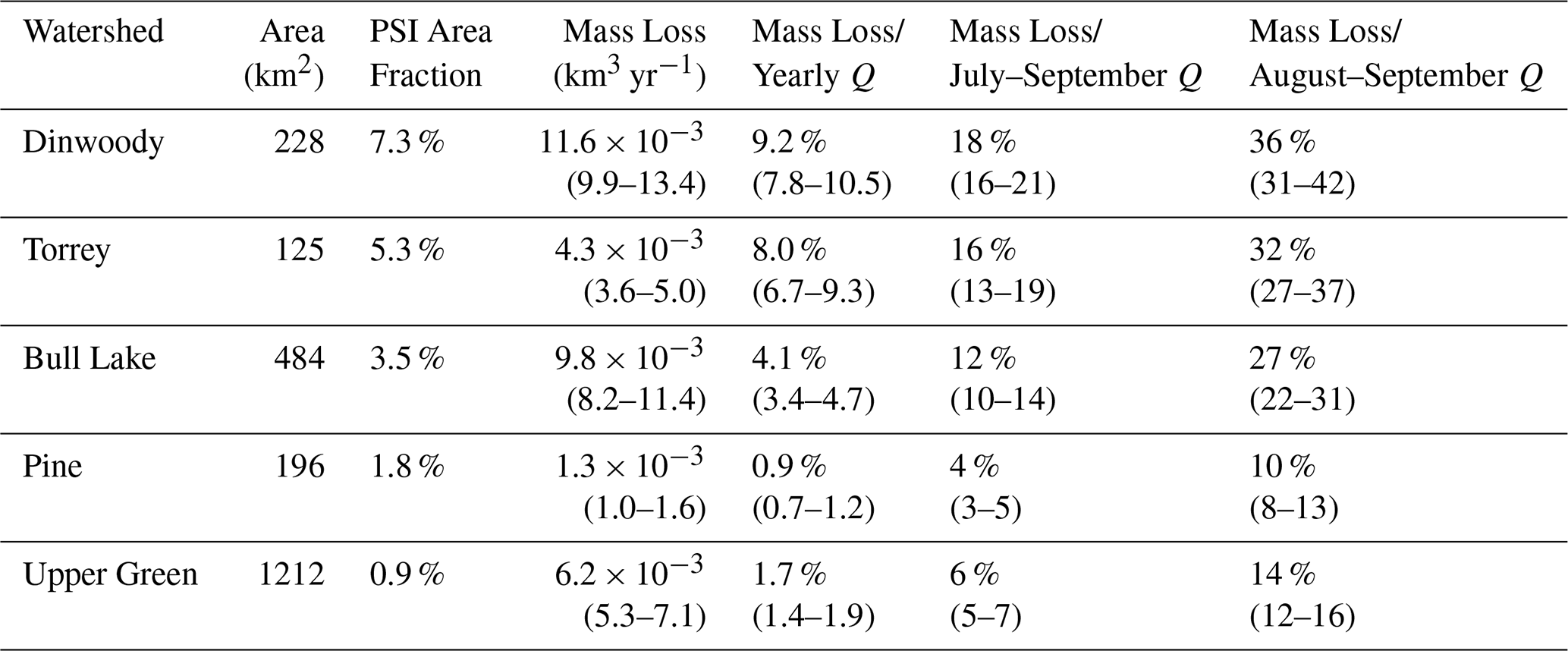
PSI mass loss contributes a sizable fraction of late-summer streamflow in the five study watersheds (Table 4). Between 17 and 18 August 2019 and 7 October 2023 PSI net mass loss in the five study watersheds averaged 3.3 × 10⁻² km³ yr⁻¹, equivalent to 3.6 % of the total annual runoff over water years 2020–2023. Due to variable PSI abundance within each watershed, PSI net mass loss contributed ∼ 1 %–2 % of the annual water yield in west-side watersheds and ∼ 4 %–9 % in east-side watersheds. Assuming that most net mass loss occurs in August and September, the PSI mass loss contribution to streamflow during that time ranges from ∼ 10 %–14 % in west-side watersheds and ∼ 27 %–36 % in east-side watersheds. Assuming a longer time period of July through September for the annual net mass loss, the average streamflow contribution during those 3 months is ∼ 4 %–6 % in west-side watersheds and ∼ 12 %–18 % in east-side watersheds. Uncertainty in the mass loss contribution varies between ±0.2 % and 1.4 % for the yearly contribution, ±1 % to 3 % for the potential July–September contribution, and ±2 % to 6 % for the potential August–September contribution.

Table 4 PSI mass loss contributions to streamflow for the five gauged study watersheds. Mass loss is estimated between 2019 and 2023, and streamflow (Q) is averaged over water years 2020 through 2023. Values in parentheses are the upper and lower uncertainty bounds.

PSI mass loss cannot fully explain spatial patterns of late-summer streamflow among WRR watersheds. Normalizing seasonal streamflow hydrographs by the May–September mean flow for each watershed reveals variations in streamflow timing (Fig. 11a). Watersheds with a higher percentage of PSI area produce relatively more late-summer streamflow (r=0.73). The common explanation for this pattern is that ice melt from the glaciers contributes “extra” streamflow in watersheds with more abundant PSI (e.g., Fountain and Tangborn, 1985; Moore et al., 2009; Nolin et al., 2010; Clark et al., 2015). Indeed, the stratification of mean August–September streamflow (normalized by total watershed area) exactly matches the ordering of watersheds by PSI area fraction (Fig. 11b). Reducing the August–September streamflow from each watershed by subtracting the estimated mass loss contribution (Table 4) provides a lower bound on streamflow patterns in the absence of PSI recession. Watersheds with more abundant PSI still produce disproportionately more streamflow in the late summer, even assuming the yearly mass loss occurs entirely in August and September (Fig. 11c). Under recent historical conditions (2005–2024 mean), Dinwoody Creek (7.3 % PSI area) and Torrey Creek (5.3 % PSI area), respectively, produce 129 % and 75 % more area-normalized August–September streamflow compared to the mean of the other three watersheds (PSI area of 0.9–3.5 %). In the lower-bound counterfactual scenario with no mass loss, Dinwoody and Torrey still produce 78 % and 45 % more area-normalized streamflow compared to the other three watersheds.

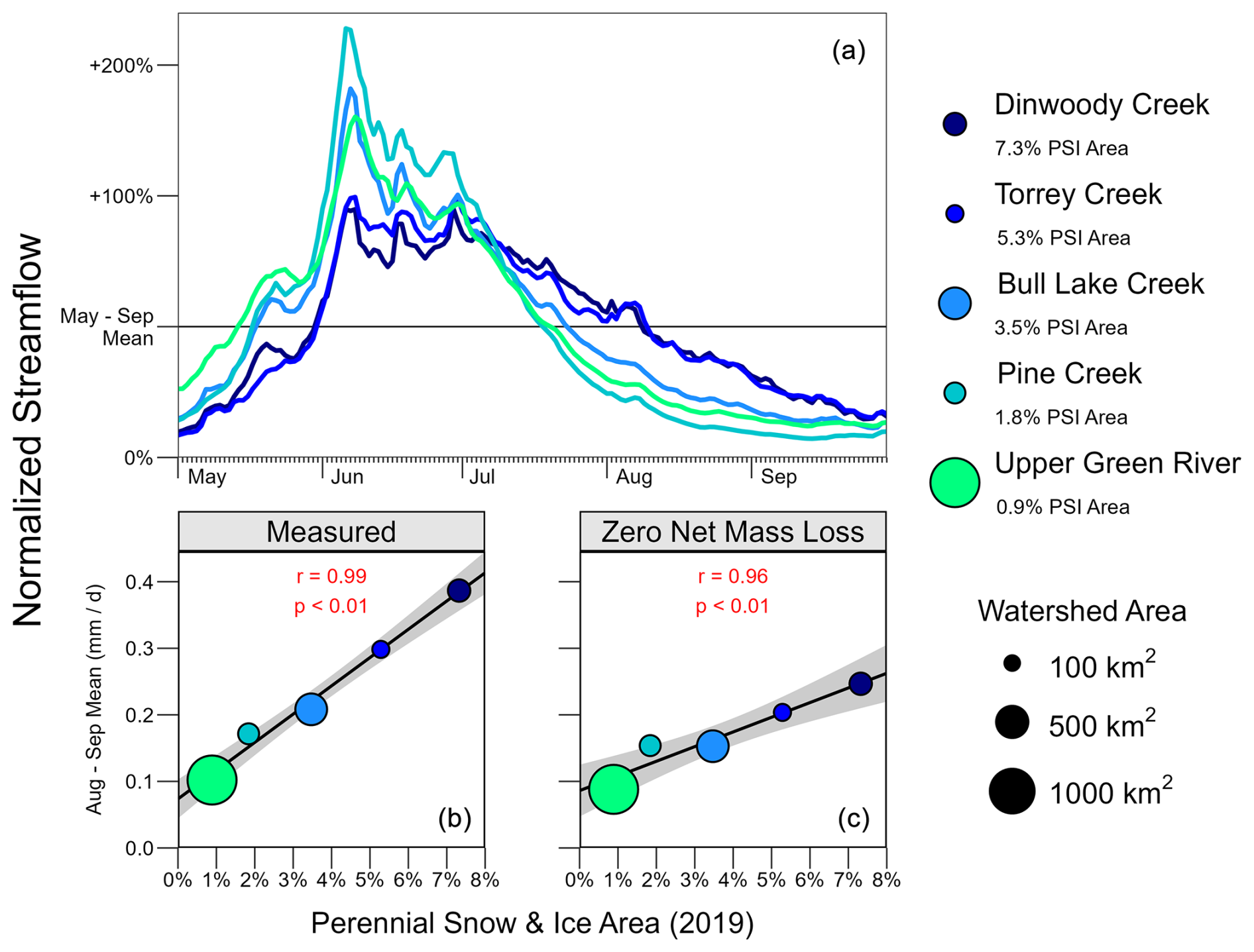
Figure 11 Normalized daily streamflow hydrographs for the five gauged study watersheds (Fig. 1). Panel (a) shows historical streamflow (2005–2024 mean) normalized by the May–September mean for each watershed. The lower panels show correlations between the fraction of watershed area covered by perennial snow and ice (PSI) and the mean daily streamflow during August and September normalized by the total watershed area. Panel (b) is averaged over water years 2020–2023 (between PSI lidar surveys), and panel (c) shows a counterfactual scenario with zero net mass loss on the same period estimated by subtracting the annual contribution of perennial snow and ice (PSI) mass loss from the measured August–September streamflow (Table 4). Correlation values show the Pearson correlation coefficient (r) and the probability that the correlation is not significant (p).

Spatial patterns of deep snow can largely explain differences in late-summer streamflow production between WRR watersheds (Fig. 12). Among the metrics considered, total snowpack volume best explains inter-watershed streamflow differences in the early melt season, from May through early July, though large inter-watershed variations remain unconstrained, potentially due to differences in elevation and aspect that control melt timing. Beginning in mid-July, deeper snow depths provide convincing explanatory metrics for streamflow patterns (Fig. 12). Snow storage in areas exceeding the 75th percentile (0.65 m) of all SWE depths on 31 May 2024 best explains inter-watershed differences in area-normalized 2005–2023 streamflow during mid-July, SWE exceeding the 90th percentile (1.26 m) best explains streamflow production from mid-July through early August, and SWE exceeding the 95th percentile (1.72 m) best explains streamflow production from mid-August into September. Streamflow production near the end of the runoff season is best correlated with SWE exceeding the 90th percentile, but this relationship may be confounded by watershed hypsometry as temperatures begin to drop below freezing in late September. The streamflow patterns in Fig. 12 are robust to the choice of time period and the imputation of streamflow data prior to water year 2022 in Torrey Creek; analogous patterns are observed using only measured streamflow from water years 2022–2024, but the shorter averaging period introduces noise due to stochastic storm events (Fig. S18 in the Supplement).

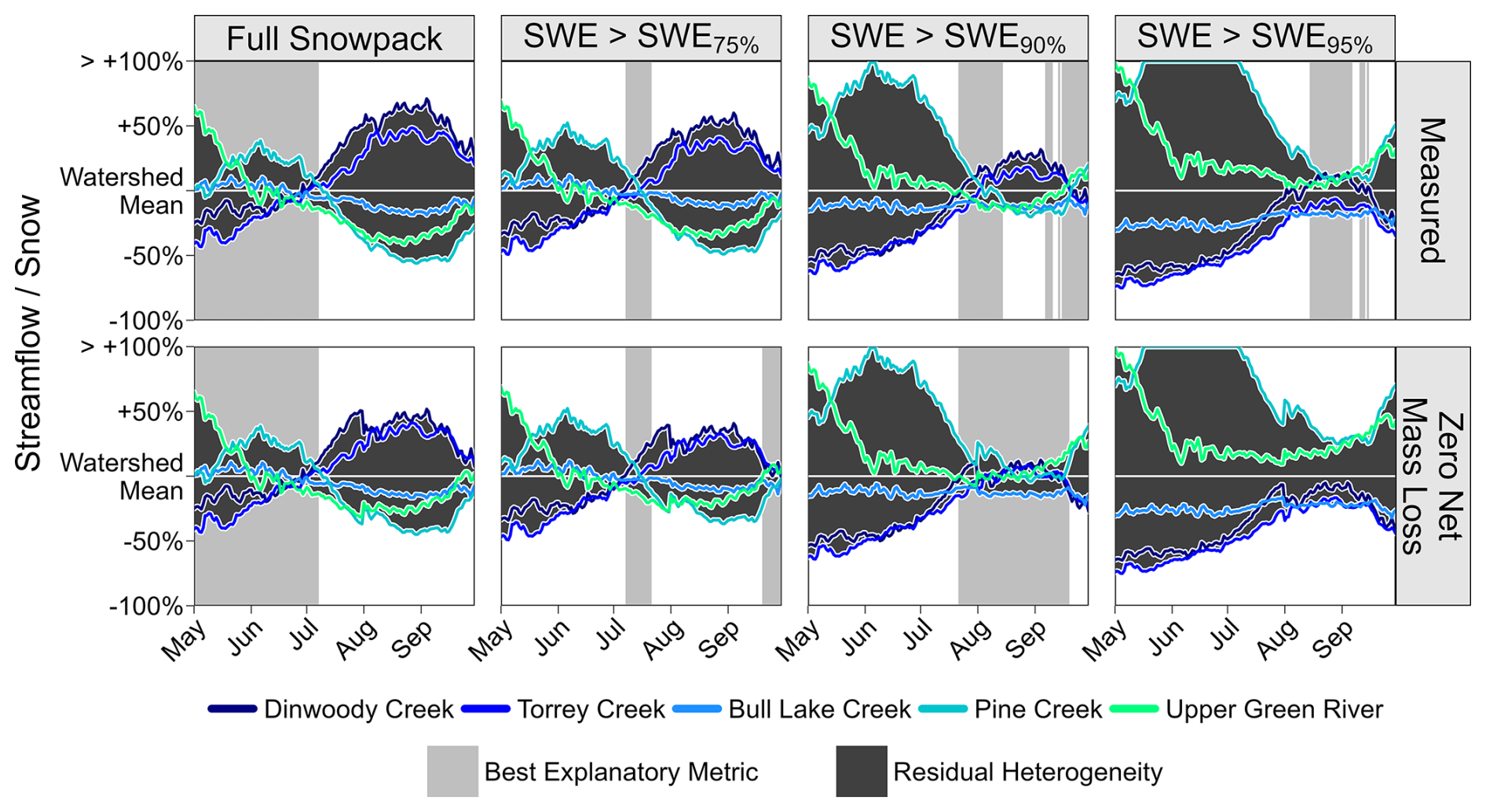
Figure 12 Time series of dimensionless streamflow metrics normalized by the cross-watershed daily average. The upper row shows historical streamflow metrics (2005–2024), and the lower row shows the same metrics assuming no net mass loss from perennial snow and ice (PSI) features. Variability between watersheds (residual heterogeneity) indicates seasonal variations in the relationship between snow storage and streamflow generation. Gray bars indicate which snowpack storage metric best explains the inter-watershed variability in streamflow at different points in the season. SWE_X% = Xth percentile SWE depth across all five watersheds; in the 31 May 2024 data, SWE_75 % = 0.65 m, SWE_90 %=1.26 m, and SWE_95 % = 1.72 m.

The combination of PSI mass loss rate and deep seasonal snow storage best explains inter-watershed streamflow patterns. Assuming no net mass loss, the > 90th percentile SWE metric best explains inter-watershed streamflow variations for the full period from late July through mid-September (Fig. 12). The relationship between historical (2005–2023) August streamflow and deeper snow storage (SWE depth > 95th percentile) is likely a result of the confounding relationship between persistent seasonal snow and PSI abundance, which makes deeper snow metrics a partial proxy for net mass loss (Fig. 10). Reducing streamflow in proportion to net PSI mass loss (Table 3) prior to calculating the hydrograph metrics accounts for this correlation between mass loss and snow persistence. After accounting for net mass loss, we observe that residual differences in late-summer streamflow generation among the watersheds (Fig. 11c) are approximately proportional to each watershed's snow storage in the deepest 10 % of the seasonal snowpack (Fig. 12).

The relationships in Figs. 11 and 12 are robust to different normalization approaches accounting for elevation, area, and snow accumulation differences among the five watersheds. Panel (a) of Fig. 11 shows that the stratification of late-summer streamflow approximately matches the fractional PSI area when each hydrograph is normalized by its mean, i.e., purely based on differences in streamflow timing. Panels (b)–(c) of Fig. 11 show a similar August–September streamflow stratification in specific discharge units (normalized by the total watershed area). Figure 12 shows similar streamflow patterns normalized by the watershed-total snowpack storage when only considering snow above 3000 m to control for different watershed sizes and gauge locations (Fig. 1). Finally, we now expand our analysis to streamflow normalized directly by the area above 3000 m, analogous to Fig. 12 but without the extra snowpack normalization step. With this elevation-dependent area-based normalization scheme, there is a negative correlation ($r=-\mathrm{0.60}$) between snowpack storage and August–September streamflow, but there is a positive correlation between August and September streamflow and the snow volume stored in areas with SWE > 1 m (r=0.63) or SWE > 2 m (r=0.88). Given the small sample size (five watersheds), only the correlation with SWE > 2 m is significant (p<0.05). The negative correlation between total snowpack storage and August–September streamflow disappears (r=0.08) when normalizing by the full watershed area instead of just the area above 3000 m due to the large separation between the contributing headwater area and the Upper Green River stream gauge (Fig. 1). However, the correlation remains negative when considering just the other four watersheds when normalizing by either the total watershed area ($r=-\mathrm{0.62}$) or the likely contributing area above the 3000 m snow line ($r=-\mathrm{0.75}$).

5 Discussion

5.1 Comparison of mass loss contributions

The 2019–2023 lidar-derived geodetic elevation change data suggest an intermediate range of PSI mass loss rates between faster and slower estimates from various methods over different time periods. Comparisons between PSI mass loss studies are complicated by interannual climate variability as well as methodological factors, including the choice of watershed(s), the seasonal time period considered, and the definition of glacier meltwater (i.e., all runoff from glaciers or net mass loss only). Nonetheless, we compare our lidar-based mass loss estimates to prior studies based on area–volume scaling relationships, isotope unmixing, and meltwater runoff measurements.

Studies using area–volume scaling relationships may underestimate the mass loss contribution to streamflow on relatively short time periods. DeVisser and Fountain (2015) use multiple area-volume scaling relationships to estimate that mass loss was equivalent to 4 %–13 % of the August–September flow in Dinwoody Creek and 2 %–6 % in Bull Lake Creek between 2001 and 2006, with upper bounds that are about 3–5 times lower than the mean contribution estimated here (Table 4). However, for an earlier period (1994–2001), the same study estimates a potential Dinwoody contribution as high as 23 %, closer to our value of 36 % for 2019–2023. Marks et al. (2015) estimate a relatively high mass loss contribution of 10 %–13 % for July–September streamflow in Bull Lake Creek for the longer 1989–2006 period, close to our 12 % estimate. Some of the variation in prior results may be attributable to episodic acceleration or slowing of PSI retreat; subjectivity in the delineation of boundaries; and effects of variable image quality, resolution, and interpretation (Thompson et al., 2011; DeVisser and Fountain, 2015). Additionally, some PSI features show vertical thinning with minimal area change between 2019 and 2023, which could cause area–volume relationships to underestimate mass loss, though precise PSI boundaries are difficult to determine in 2019 and 2023 due to variable snow cover at the time of both lidar acquisitions.

Conversely, studies based on isotope unmixing and discharge measurements may be prone to overestimation of mass loss contributions to streamflow if the contribution of supraglacial snowmelt is neglected. Cable et al. (2011) estimate a mass loss contribution to August streamflow as high as 70 % in 2007 and 53 % in 2008 for Dinwoody Creek, as much as 1.9 times higher than our August–September estimate. Similarly, Vandeberg and VanLooy (2016) estimate a PSI mass loss contribution of 81 %–83 % to Torrey Creek streamflow in August 2014 based on isotope unmixing from Continental Glacier meltwater. VanLooy and Vandeberg (2024) provide a lower estimate of 37 % for August 2019 streamflow using similar methods. These Torrey Creek estimates range from 1.2 to 2.6 times higher than the August–September contribution estimated here (32 %). In the Bull Lake Creek watershed, VanLooy and Vandeberg (2019) estimate an August 2015 streamflow contribution of 56 % based on direct measurements of discharge below major glaciers. This is 2.1 times higher than our August–September estimate here, but 2015 exhibited a particularly low summer snowpack with mostly bare ice exposed on the glaciers, potentially leading to a larger mass loss contribution to streamflow (Jeffrey VanLooy, personal communication, October 2024).

Studies based on sampling meltwater below glaciers, whether for isotope analysis or by direct discharge measurement, may be affected by uncertain estimates of endmembers and potentially confounded by meltwater derived from lingering supraglacial snow that is not treated separately from multi-year mass loss. Notably, the lower Torrey Creek streamflow contribution (37 %) found by VanLooy and Vandeberg (2024) is based on ice samples from bare glacier ice compared to the higher contribution (81 %–83 %) based on meltwater at the glacier's terminus (Vandeberg and VanLooy, 2016), although melt and runoff rates also varied between the sampling years. The large contribution of total meltwater from PSI locations, as opposed to solely net mass loss from ice, is consistent with prior analyses (Bell et al., 2012) and supports our observation that PSI features coincide with persistent seasonal snow zones. Trace element measurements similarly support a distinction in the sources of supraglacial meltwater and proglacial streams in the WRR (Barkdull et al., 2021).

5.2 Spatial heterogeneity

Topography plays a crucial role in mediating snow persistence and annual mass loss in the WRR. With 338 distinct PSI features available for analysis, we are able to identify endmembers that exemplify particular topographic controls (Fig. 8). A simple linear classification of dominant topographic factors for the entire PSI area quantifies the importance of wind drifting for deep snow accumulation (Fig. 9). The most hydrologically resilient WRR PSI features (low mass loss contribution) typically benefit from a combination of shading and wind drifting, which combine to create topographic refugia where accumulation is enhanced and ablation is limited (e.g., Fig. S15a1–a3 in the Supplement). While we implicitly incorporate the role of avalanching from cirque headwalls in the upwind area index (Appendix C, Eq. C6), we do not isolate the role of avalanches in this study, which may be particularly important for small, resilient PSI features (e.g., Laha et al., 2017; Onaca et al., 2022). Spatiotemporal albedo variations also modulate the effect of shading and solar insolation on PSI mass loss (e.g., Wolken, 2000; Davaze et al., 2018; Owusu-Amponsah et al., 2023). Future research could explore additional processes controlling mass balance heterogeneity and investigate the interaction of topographic factors identified here through multivariate statistical analysis (e.g., Florentine et al., 2020), distributed field measurements (e.g., Hannah et al., 2000), or numerical simulations of topographic controls (e.g., Kessler et al., 2006).

Spatial heterogeneity in the PSI mass loss contribution requires caution in the extrapolation of field measurements to the watershed scale. Discrepancies between this study and some prior estimates of the mass loss contribution to streamflow may be partially explained by selective sampling of the largest, most notable glaciers (e.g., Marston et al., 1991; Vandeberg and VanLooy, 2016). Relatively large glaciers (area > 0.5 km²) exhibit faster mass loss rates (Table 3) and reduced variability compared to the full diversity of PSI features (Figs. 6 and 7). Complete spatial coverage by airborne lidar surveys can reduce uncertainty in the PSI mass loss contribution to streamflow by mapping all snow and ice storage changes, directly constraining spatial variability and accounting for numerous features smaller than the 0.01 km² threshold adopted for manual polygon delineation (Fountain et al., 2023). Between 2019 and 2023, PSI features <0.01 km² contributed 12 % of all net mass loss in the study area (Table 3), suggesting that perennial snow patches (e.g., Fig. 3f) could be an important source of meltwater despite being too small for manual delineation.

About 6 % of all WRR net mass loss derives from buried ice, which includes debris-mantled glacier margins excluded from polygon delineation (e.g., Figs. 3e and 1 of Fountain et al., 2023) as well as several ice-cored moraines (Fig. S6 in the Supplement). Detecting these buried ice features is a strength of our lidar-based approach to mass estimation. With spatially complete elevation change data, we can identify buried ice features wherever patterns of elevation change are spatially coherent and consistent with surface morphology. This change-based approach to PSI detection largely avoids the problem of deciding which areas to include in PSI net mass loss calculations, thereby respecting the glacier–rock glacier continuum (Anderson et al., 2018). Delineating buried ice features based on visible surface cover in areas with coherent elevation change supports the hypothesis that buried ice and rock glaciers are more resilient to the current warmer climate compared to nearby surficial features (Jones et al., 2019), with slower mass loss rates than glaciers and snowfields despite less snow accumulation (Fig. 7 and Table 3).

5.3 Interrelationship of snow drifts, glaciers, and streamflow

Watersheds with the most deep snow storage also have the most abundant PSI features, the largest mass loss contributions, and the highest late-summer streamflow. Figure 13 summarizes key correlations considering a streamflow generation metric defined by the mean August–September streamflow relative to the 31 May 2024, seasonal snow volume above 3000 m (to control for gauge location). This metric (vertical axis of Fig. 13) is effectively a seasonal subset runoff efficiency relative to the initial snowpack. Adjacent WRR watersheds with more area-average snowpack storage (above 3000 m) at the start of the melt season counterintuitively produce less late-summer runoff ($r=-\mathrm{0.82}$, p<0.1). Wind drifting explains this unexpected inverse relationship. Watersheds with favorable topography develop more abundant deep snow drifts (Figs. 9 and 10), which persist through the summer and explain inter-watershed streamflow variations later in the melt season (Fig. 12). Consequentially, late-summer streamflow generation correlates positively with very deep snow storage (r=0.97, p<0.01 for SWE > 2 m), reversing the negative correlation with total area-normalized seasonal snow. However, the strong correlation between watershed-total PSI mass loss and SWE > 2 m (r=0.94, p<0.02) confounds a purely correlation-based interpretation. Indeed, there is an almost identical correlation between late-summer streamflow generation and net mass loss from PSI (r=0.97, p<0.01).

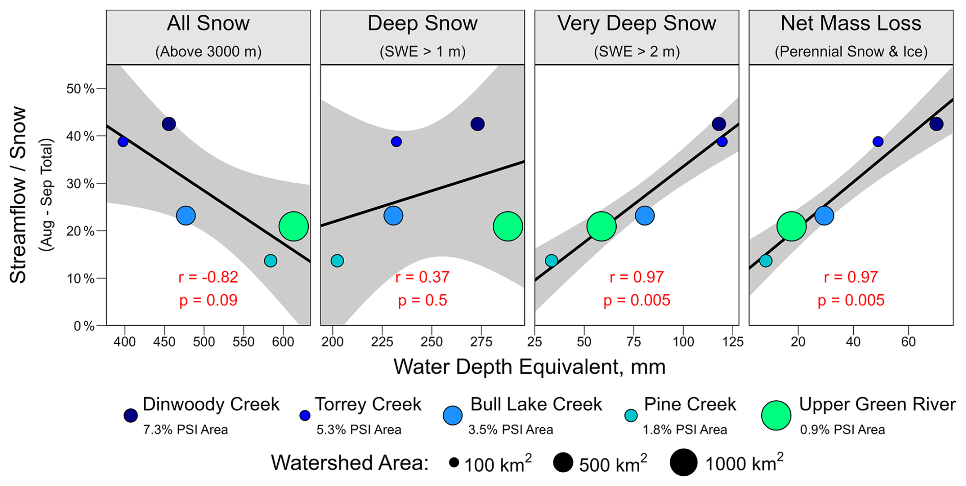
Figure 13 Correlations between normalized August and September streamflow and various snow or mass loss metrics across the five study watersheds. Streamflow (vertical axis) is normalized by the volume of snow (above 3000 m) in each watershed on 31 May 2024, which is the same survey used to calculate all snow metrics. Streamflow and mass loss are averages across water years 2020–2023. Correlation values show the Pearson correlation coefficient (r) and the probability that the correlation is not significant (p). All metrics shown here are normalized by the area above 3000 m in each watershed to control for different watershed sizes and gauge locations (Fig. 1).

After subtracting the net mass loss contribution, the stratification of watersheds by late-summer streamflow remains nearly unchanged (Fig. 11b–c), so we conclude that deep snow patterns are necessary to explain streamflow patterns (Fig. 12). The importance of deep snow for late-summer streamflow is well recognized (Luce et al., 1998; Winstral et al., 2013; Brauchli et al., 2017; Le et al., 2023), but our WRR lidar data provide a unique opportunity to quantify the role of deep snow storage in shaping hydrographs across multiple watersheds using purely data-driven methods (Figs. 10–12). Delayed snowmelt runoff from watersheds with deeper snow can increase the climate resilience of downstream communities by mitigating the effects of snow drought, which is especially important in areas such as the WRR, where artificial storage capacity is limited (McNeeley et al., 2018; Gordon et al., 2024).

Additional hydrological processes may further mediate late-summer streamflow differences, though snow- and ice melt appears to be the dominant driver. Groundwater can introduce timing lags between melt and streamflow generation, and spatial heterogeneity in the subsurface can create streamflow timing differences between watersheds (Huntington and Niswonger 2012; Cochand et al., 2019; Somers and McKenzie, 2020). Thus, part of the difference in WRR streamflow timing (Fig. 11a) could plausibly result from differences in groundwater transit times. However, the largest and second-smallest watershed both have similar streamflow patterns (Upper Green River and Pine Creek), which suggests that our conclusions are insensitive to the flow path distance between the snowmelt area and the stream gauge. Other potential sources of late-summer streamflow variability include differences in riparian evapotranspiration (Graup et al., 2022), elevation-mediated differences in snowmelt timing that can affect evapotranspiration (Barnhart et al., 2016), and differences in lake storage that can buffer streamflow (Arp et al., 2006). Additionally, an unmeasured amount of water is diverted from the Upper Green River above the gauging location for local irrigation. Nevertheless, the relationship between snow, PSI, and late-summer streamflow is robust to different normalization metrics and the exclusion of one or more of the watersheds (Figs. 10–13), and the broader context of the snowy WRR supports our interpretation that snow and ice melt is the dominant factor controlling late-summer streamflow.

Landscape-scale wind interactions with snow exert a large control on the WRR water balance. Topographic shelter and the size of upwind contributing areas are the dominant controls on deep snow accumulation in the WRR from the grid cell scale (Fig. 9) to the watershed scale (Fig. 10). A new snow drift index based on the extent of potential upwind contributing area shows that some PSI features in the WRR could collect snow from an upwind contributing area as large as several square kilometers, roughly 1–2 orders of magnitude larger than the area of the resultant drift zone. These kilometer-scale contributing areas are consistent with the estimation of Outcalt and MacPhail (1965) for a drift glacier in a similar environment. Concentration of drifting snow from a large contributing area leads to lidar-measured snow depths of 6–12 m (∼ 3–6 m SWE) over a contiguous area larger than 0.1 km² in some areas (e.g., Fig. 5a2). In the WRR, blowing snow accumulated over extensive plateau surfaces (e.g., Fig. 8d4) may decouple drift depths from more conventional topographic wind indices, such as the upwind angle of Winstral et al. (2002). Spatial precipitation fields in alpine mountains remain highly uncertain (Henn et al., 2018), and it is possible that the greater total snowpack storage in west-side WRR watersheds is entirely a result of orographic precipitation (Table 1). Nevertheless, the combination of more abundant deep drifts and reduced total snowpack storage in downwind watersheds (Fig. 10) could suggest a potential effect of sublimation during wind transport in the more heavily drifted watersheds.

PSI abundance in the WRR is the result of hysteresis from legacy climate conditions that permitted glacier growth in sufficiently cold and snowy areas (Meier, 1951; Matthews and Briffa, 2005). As glaciers retreat, they recede into cirques and can transition into perennial or seasonal snowfields. Throughout this transition, topographic controls on the mass balance become increasingly dominant (Florentine et al., 2018). In the WRR, the most hydrologically resilient glaciers and snowfields (low mass loss contribution) have relatively deep seasonal snow accumulation (Fig. 7), which is associated with topographic controls on wind drifting (Fig. 9). Paradoxically, watersheds with the most resilient PSI features may have a larger mass loss contribution to streamflow during late stages of deglaciation simply by virtue of retaining more PSI features for longer. This relationship is evident in the positive correlation (r=0.94) between watershed-average seasonal snow storage in areas with SWE > 2 m and watershed-average net mass loss (Fig. 10). In contrast, the west-side (upwind) WRR watersheds supported much larger ice sheets than the east-side (downwind) watersheds during the Pleistocene glacial maximum since orographic precipitation favors glaciation on the upwind aspect when the mountain range is below the ELA (Birkel et al., 2012). The greater extent of west-side ice sheets during glacial maxima could reduce topographic relief on the upwind side of the mountain range (Birkel et al., 2012), intensifying the present-day disparity in topographic refugia and associated PSI patterns between upwind and downwind watersheds (Fig. 10).

Since perennial snow and ice features roughly coincide with the most persistent areas of the seasonal snowpack, the relationship between mass loss and streamflow is confounded by seasonal snowmelt. Watersheds with the largest fraction of PSI features by area have the greatest potential for streamflow reductions post-glaciation (Table 4), but these same watersheds will likely continue to produce considerably more area-normalized late-season streamflow compared to the other watersheds as a result of deep seasonal snow (Fig. 12). Incorrectly assuming that WRR watersheds would all behave similarly without PSI mass loss leads to a 45 %–78 % underestimation of August–September streamflow in the most glaciated watersheds even in the conservative post-deglaciation counterfactual scenario (Fig. 11c). Although PSI abundance and deep snow are strongly correlated at the watershed scale (Fig. 10), some of the larger glaciers have clearly separated accumulation and ablation zones, with little to no supraglacial snow accumulation in the ablation zone (e.g., Fig. 5b2). Thus, our conclusion linking deep snow to PSI abundance is only valid at the watershed scale, and a smaller-scale analysis would need to account for the effects of glacier flow.

In the WRR, inter-watershed patterns of glaciation and streamflow are both mediated by the interaction of wind and snow with topography. Spatial patterns of streamflow generation (i.e., differences between watersheds) are relatively robust to a post-deglaciation scenario in the WRR (Fig. 11b–c) because of topographic factors that enhance snow accumulation and persistence (Figs. 9–10), which appear to be a substantial control on streamflow timing (Fig. 12). Wind transport of snow has been recognized as a dominant control on watershed-scale patterns of WRR glaciation for the past 8 decades (Baker, 1946), but quantifying this interrelationship at a high resolution reveals that wind will likely remain a salient driver of seasonal snow persistence and streamflow patterns even in a future with fewer glaciers.

5.4 Transferability

Since most mountain ranges do not have multiple years of high-resolution lidar data, directly extending our methods to additional areas would require a substantial data collection effort. We caution against a direct application of the topographic indices discussed here in a predictive framework without observed geodetic elevation data, i.e., attempting to predict snow or PSI change based on, for example, the wind indices. Although we have shown that most deep snow is associated with favorable topography for wind drifting (Fig. 9), the opposite is not true, and there are many areas with very little snow that nevertheless happen to be wind-sheltered (e.g., Fig. S15a2). Predicting unobserved snow accumulation patterns is notoriously challenging (Dozier et al., 2016), but interpreting the likely topographic controls on an observed snowpack pattern (as done here) is comparatively straight-forward. In areas lacking lidar data, relationships between PSI retreat and snow persistence might still be elucidated from optical remote sensing, e.g., satellite-based snow cover persistence or similar metrics (Selkowitz and Forster, 2016; Hammond et al., 2018).

Although our methodological approach requires intensive data collection, our conclusions are more easily generalizable. We expect that the interrelationship between seasonal snow persistence, PSI net mass loss, and streamflow identified here will generalize to other alpine mountain ranges undergoing glacier recession. In mountain areas with relatively small glaciers close to the regional ELA, it is widely observed that topographic controls (wind drifting, shading, etc.) become increasingly important as glaciers retreat (Graf, 1976; Hoffman et al., 2007; Florentine et al., 2018; Mott et al., 2019; Onaca et al., 2022). Larger glacier systems extending considerably above the ELA (e.g., High-Mountain Asia) are intuitively less likely to be influenced by small-scale topographic controls. Thus, we expect that the strong mutual correlations between deep seasonal snow, PSI mass loss, and late-summer streamflow (Fig. 13) are transferable to mountain ranges near the ELA under a warming climate. The correlation between deep snow and PSI abundance (Figs. 10, 11b) should also generalize to mountains near the ELA even under stable climate conditions.

6 Conclusions

Glaciers are often conceptualized as a driver of hydrological differences between mountain watersheds, but they are also an indicator of spatial heterogeneity in processes controlling snow persistence. Due to the causal relationship between snow persistence and glacier formation, the accumulation zones of mountain PSI features necessarily coincide with the most persistent areas of the seasonal snowpack. Inter-watershed patterns of glaciation and streamflow production can both result from topographic mediation of the underlying processes that drive snow persistence, such as wind drifting and shading. Our observations in the WRR suggest that some mountain glaciers are more a result, rather than a driver, of hydrological heterogeneity. Consequentially, deglaciating WRR watersheds that currently exhibit elevated late-summer streamflow production will likely continue to out-produce nearby watersheds because seasonal snowpack dynamics control streamflow timing. Although climatic disruptions such as a rain–snow transition could reduce the role of snow persistence in shaping hydrographs, we expect inter-watershed streamflow patterns to remain especially robust in cold, windy regions, such as the WRR. Greater synergy between research efforts in mountain glaciology and snow hydrology is needed to further explore the interrelationships between snow and ice storage cycles and forecast their response to climate change.

Appendix A: Description of empirical snow density model

Based on the graphical analysis of partial regression residuals as discussed in Sect. 3.2, we posit an additive model of bulk snow density driven by three independent factors:

$$\begin{array}{}\text{(A1)}& {\mathit{\mu }}_{\mathrm{Density}}=f_{\mathrm{1}}+f_{\mathrm{2}}+f_{\mathrm{3}}.\end{array}$$

The first factor includes a constant offset and scales linearly with snow depth:

$$\begin{array}{}\text{(A2)}& f_{\mathrm{1}}=c_{\mathrm{1}}+c_{\mathrm{2}}\times \mathrm{Depth}.\end{array}$$

The second factor is a generalized logistic function of elevation describing a smooth threshold (interpreted as the ripening elevation near the 0 °C isotherm) where snow densifies most rapidly:

$$\begin{array}{}\text{(A3)}& f_{\mathrm{2}}={\displaystyle \frac{c_{\mathrm{3}}}{\mathrm{1}+e^{-c_{\mathrm{4}}\times \left(\frac{\mathrm{Elevation}-\mathrm{3000}}{\mathrm{1000}}-c_{\mathrm{5}}\right)}}}.\end{array}$$

The third factor is a rectangular hyperbola that reduces density with increased canopy cover:

$$\begin{array}{}\text{(A4)}& f_{\mathrm{3}}=c_{\mathrm{6}}\times \left(\mathrm{1}-{\displaystyle \frac{c_{\mathrm{7}}}{c_{\mathrm{7}}+\text{Canopy Cover}}}\right).\end{array}$$

We use Bayesian sampling to generate parameter estimates assuming a normal error distribution with standard deviation σ:

$$\begin{array}{}\text{(A5)}& \text{Density}\sim \text{normal}\left({\mathit{\mu }}_{\mathrm{Density}},\mathit{\sigma }\right).\end{array}$$

Median values of 100 Bayesian samples for each parameter obtained by fitting 39 regional density measurements: c₁=0.57, c₂=0.015, $c_{\mathrm{3}}=-\mathrm{0.22}$, c₄=6.3, c₅=0.32, $c_{\mathrm{6}}=-\mathrm{0.14}$, c₇=0.060, and σ=0.026.

Taking the derivative of Eq. (A3) and substituting median parameter values, we note that the fastest rate of density change corresponds to an elevation of 3320 m, consistent with regional observations of snow temperature, which indicate an isothermal elevation of ∼ 3300 m.

An interactive version of the empirical density model is available online at https://www.desmos.com/calculator/n54vbqb2qc (last access: 15 August 2025​​​​​​​).

Appendix B: Description of a deep neural network for SWE imputation

As explained in Sect. 3.3, we use a deep neural network implemented in PyTorch (Paszke et al., 2019) to impute SWE at 3 m resolution for the portion of the Upper Green River watershed that is outside the lidar survey area (Fig. S1 in the Supplement).

The following data are used as prediction features:

1. elevation (3 m resolution; all DEM derivatives also at 3 m resolution unless indicated);

2. north apparent dip (combines slope and aspect);

3. east apparent dip (combines slope and aspect);

4. topographic roughness index (mean absolute elevation difference relative to surrounding cells);

5. topographic position index (elevation difference relative to mean of surrounding cells);

6. topographic curvature at 3 m resolution;

7. topographic curvature at 30 m resolution, interpolated back to 3 m;

8. topographic curvature at 300 m resolution, interpolated back to 3 m;

9. fractional canopy cover from RCMAP (Rigge et al., 2021), interpolated from 30 to 3 m;

10. Landsat fractional snow cover (fSCA), mean of 16 cloud-free observations, March–October 2020–2024;

11. Landsat fractional snow cover (fSCA), same day as lidar data (31 May 2024);

12. upwind angle (Sx, Winstral et al., 2002);

13. upwind area index (Appendix C);

14. mean annual sun exposure time (topographic shading).

The model structure consists of these 14 input features, a ReLU layer of 10 000 neurons, dropout regularization (p=0.5), and 9 subsequent ReLU layers of 100 neurons each, with a single final linear neuron predicting SWE. The model is trained using the Adam optimizer (Kingma and Ba, 2017) with a batch size of 256, learning rate of 3 × 10⁻⁴, and CUDA GPU acceleration. Data are split into halves based on a 1 km square grid to avoid spatial autocorrelation. Half of the 1 km square areas are used for training with 10⁶ random samples from within the training areas. The other half of 1 km squares are used for validation and test sets, with 5 × 10⁵ random samples each. We implement early stopping if the coefficient of variation (R²) on the validation set falls at least 0.01 below the maximum achieved R² for 10 epochs. In this case, early stopping ended training after 64 epochs, with a validation R² of 0.679 for SWE at 3 m resolution.

SWE depth is imputed using the trained model with the same 14 features. Snow presence is masked using a random forest classifier (Breiman et al., 2002) trained on the same 14 features with 200 decision trees. The out-of-bag error rate for the snow presence classification is 7 %. The final R² is 0.683 for SWE at 3 m resolution on the test set.

Appendix C: Definition of the upwind area snow drift index

Let (x, y) refer to the Cartesian coordinates of an arbitrary grid cell, and let (x_i, y_i) refer to the coordinates of a local grid cell for which we will calculate the snow drift contributing area. Let (r, θ) refer to the polar coordinates at distance r along the θ azimuth from a given grid cell.

First, we define the upwind fetch distance (Lapen and Martz, 1993) for a given cell, D_fetch, as the minimum distance r along the upwind azimuth θ from the coordinates (x, y), satisfying Eq. (C1), where S_min defines a minimum upwind angle:

$$\begin{array}{}\text{(C1)}& \begin{array}{rl}{D}_{\mathrm{fetch}}\left(x,y\right)& \equiv min\left\{r\mathrm{|}\mathrm{Elevation}\left(r,\mathit{\theta }\right)\ge \mathrm{Elevation}\left(x,y\right)\right.\\ & \left.+\tan \left(S_{\min }\right)\times r\right\}.\end{array}\end{array}$$

D_fetch is thus the minimum distance to a “meaningful” upwind terrain obstacle in the θ direction.

Next, we calculate D_fetch for all cells along the azimuth θ from (x_i, y_i) and apply a binary threshold such that an upwind cell is defined as “wind-exposed” if its D_fetch is greater than some minimum distance MinD_fetch:

$$\begin{array}{}\text{(C2)}& \mathrm{Exposure}(r,\mathit{\theta })\equiv \left.\begin{array}{l}\mathrm{0},D_{\mathrm{fetch}}(r,\mathit{\theta })<{\mathrm{MinD}}_{\mathrm{fetch}}\\ \mathrm{1},D_{\mathrm{fetch}}(r,\mathit{\theta })\ge {\mathrm{MinD}}_{\mathrm{fetch}}\end{array}\right\}.\end{array}$$

Note that Exposure is defined along an azimuth (r, θ) from the local cell (x_i, y_i), but D_fetch as used in Eq. (C2) is calculated relative to the outlying coordinates of (r, θ), such that (x, y) in Eq. (C1) is obtained from $x=x_i+r\times \cos \left(\mathit{\theta }\right),y$ = $y_i+r\times \sin \left(\mathit{\theta }\right)$, with r reset to 0 for all (x, y) in Eq. (C1).

Not all upwind exposed areas can contribute to snow accumulation at (x_i, y_i) since intervening sheltered zones may trap snow and prevent further transport. Sheltered zones are defined by a minimum continuous unexposed distance, MinD_shelter. We define a maximum contributing distance r_max along a given azimuth based on the closest upwind sheltered zone, not counting the local sheltered zone containing (x_i, y_i). Thus, an upwind sheltered area interrupts the line search if and only if the search has previously encountered at least one closer exposed area:

$$\begin{array}{}\text{(C3)}& r_{\max }\left(\mathit{\theta }\right)\equiv min\left\{r\left|\begin{array}{l}\underset{r}{\overset{r+{\mathrm{MinD}}_{\mathrm{shelter}}}{\int }}\mathrm{Exposure}\left(r,\mathit{\theta }\right)\times \mathrm{d}r=\mathrm{0}\\ \wedge \underset{\mathrm{0}}{\overset{r}{\int }}\mathrm{Exposure}\left(r,\mathit{\theta }\right)\times \mathrm{d}r>\mathrm{0}\end{array}\right.\right\}.\end{array}$$

In practice, the continuous integrals in Eq. (C3) are replaced with a run length encoding of the Exposure vector derived from the discrete grid cells along the upwind azimuth from (x_i, y_i). Thus, r_max(θ) is the distance to the start of the first continuous run of unexposed cells exceeding the MinD_shelter length that is after the first run of exposed cells. An upper bound on r_max, denoted as MaxD_contrib, may be useful to prevent unreasonably long-distance wind transport in some cases.

Finally, we integrate the potential contributing area within an upwind angular sector defined by [θ_min, θ_max] and the maximum contributing distance along each azimuth r_max(θ) from (x_i, y_i). In polar coordinates, the area integral is given by

$$\begin{array}{}\text{(C4)}& \mathrm{Area}=\int \int \mathrm{d}A=\int \int r\times \mathrm{d}r\mathrm{d}\mathit{\theta }.\end{array}$$

By counting only exposed areas (defined by Eq. C2) and adding definite integral bounds from definitions introduced earlier, we arrive at the formula for the potential upwind contributing area:

$$\begin{array}{}\text{(C5)}& \begin{array}{rl}\text{Contributing Area}\left(x_i,y_i\right)& ={\int }_{{\mathit{\theta }}_{\min }}^{{\mathit{\theta }}_{\max }}{\int }_{\mathrm{0}}^{r_{\max }\left(\mathit{\theta }\right)}\mathrm{Exposure}\left(r,\mathit{\theta }\right)\\ & \times r\times \mathrm{d}r\mathrm{d}\mathit{\theta }.\end{array}\end{array}$$

Since snow transported from a more distant location is less likely to be deposited at (x_i, y_i) due to a combination of sublimation and upwind drifting, we weight the contributing area by the transport distance from the closest exposed zone to (x_i, y_i). Portions of the downwind length integral with a topographic slope, Slope(r, θ), greater than S_steep are not counted towards the transport distance because mechanisms other than wind (i.e., avalanching) can redistribute snow from steep slopes. Thus, the drift deposition distance is defined using a helper function NonSteep(r, θ), which zeros out the length integral over steep slopes:

$$\begin{array}{}\text{(C6)}& {\displaystyle }\mathrm{NonSteep}(r,\mathit{\theta })\equiv \left\{\begin{array}{l}\mathrm{0},\mathrm{Slope}\left(r,\mathit{\theta }\right)\ge S_{\mathrm{steep}}\\ \mathrm{1},\mathrm{Slope}\left(r,\mathit{\theta }\right)<S_{\mathrm{steep}}\end{array}\right.,\text{(C7)}& {\displaystyle }\begin{array}{rl}\text{Deposition Distance}\left(\mathit{\theta }\right)& \equiv {\int }_{\mathrm{0}}^{min\left\{r\mathrm{|}\mathrm{Scour}\left(r,\mathit{\theta }\right)=\mathrm{1}\right\}}\mathrm{NonSteep}\left(r,\mathit{\theta }\right)\\ & \times \mathrm{d}r.\end{array}\end{array}$$

A scale factor related to deposition downwind of the contributing area along a given azimuth is defined using an exponential function with a halving distance of HalfD_drift:

$$\begin{array}{}\text{(C8)}& \text{Deposition Factor}\left(\mathit{\theta }\right)\equiv e^{\frac{\ln \left(\mathrm{2}\right)}{{\mathrm{HalfD}}_{\mathrm{drift}}}\times \text{Deposition Distance}\left(\mathit{\theta }\right)}.\end{array}$$

The upwind area index is obtained by combining Eqs. (C5) and (C8):

$$\begin{array}{}\text{(C9)}& \begin{array}{rl}\text{Upwind Area Index}\left(x_i,y_i\right)& \equiv {\int }_{{\mathit{\theta }}_{\min }}^{{\mathit{\theta }}_{\max }}{\int }_{\mathrm{0}}^{r_{\max }\left(\mathit{\theta }\right)}{\displaystyle \frac{\mathrm{Exposure}\left(r,\mathit{\theta }\right)}{\text{Deposition Factor}\left(\mathit{\theta }\right)}}\\ & \times r\times \mathrm{d}r\mathrm{d}\mathit{\theta }.\end{array}\end{array}$$

Free parameters required to calculate the upwind area index are tabulated as follows: [θ_min, θ_max] is the upwind azimuth range, S_min is the minimum upwind shelter angle to define fetch distance, MinD_fetch is the minimum upwind fetch distance to classify a given location as wind-exposed, MinD_shelter is the minimum continuous unexposed distance that interrupts wind transport, MaxD_contrib is (optional) an upper bound on the maximum wind transport distance, S_steep is the minimum terrain slope above which downwind transport distance is ignored, and HalfD_drift is the exponential halving distance for downwind snow deposition.

Values used in the present study are as follows: [θ_min, θ_max] is 240 to 300° (west ±30°, conservatively large range obtained from weather data and observed drifts), S_min is 7° (obtained by testing several thresholds for agreement with observed drifts), MinD_fetch is 1000 m (minimally sensitive: most cells have Fetch = grid res. or Fetch → Inf), MinD_shelter is 500 m (obtained from measurement of observed drift patterns), MaxD_contrib is 5000 m (minimally sensitive: r_max(θ) is usually fixed by MinD_shelter in Eq. C3), S_steep is 45° (obtained from observed drift locations relative to the slope of cirque walls), and HalfD_drift is 500 m (obtained from measurement of observed drift patterns).