Factors influencing lake surface water temperature variability in West Greenland and the role of the ice sheet

Subarctic West Greenland is populated by thousands of seasonally ice-free lakes. Using remotely sensed observations, we analyse the surface water temperatures of six lakes during 1995–2022 to identify factors influencing their variability. The connectivity to the Greenland Ice Sheet (GrIS) has a clear influence on lake surface temperature, with ice-sheet-marginal lakes experiencing smaller average summer maximum temperature (<6 °C) and minimal interannual variability. A lake fed by a GrIS-originating river has the fastest seasonal response and largest seasonal amplitude with average maximum temperatures above 13 °C. The seasonal cycle of surface water temperature for all studied lakes is asymmetrical, with faster warming observed after ice-off and a slower cooling of water towards winter freezing. We find that during the study period, the onset of positive stratification occurred earlier, at rates of up to 0.5 d yr⁻¹, and that July–August temperatures increased at rates up to 0.1 °C yr⁻¹, although the GrIS-connected lakes show smaller increases. Our analysis suggests that the main meteorological factor determining interannual variability of surface water temperature in the studied lakes is air temperature. This study highlights the important role of remote sensing for long-term monitoring of Greenland lakes under climate change.

1 Introduction

The subarctic expanse of West Greenland is home to a multitude of lakes (How et al., 2021), their seasonal ice-free periods providing a window into the region's dynamic environmental processes (Anderson et al., 2017; Fowler et al., 2020). Influenced by climatic and glacial factors, these water bodies offer invaluable insights into the intricate interplay of climatic forces shaping high-latitude ecosystems (Saros et al., 2019, 2023; Prater et al., 2022). Among the myriad consequences of climate change for these lakes, one of the most pressing concerns is the direct and indirect impacts of rising lake surface water temperature (LSWT). This phenomenon not only affects various ecological states, structures, and processes (Williamson et al., 2009; Woolway et al., 2022) but also holds implications for ice sheet mass balance (Zhang and Bolch, 2023). Specifically, the interaction between lakes and the ice margin involving lake–ice processes such as calving (Mallalieu et al., 2021; Minowa et al., 2023), submarine melting (Sugiyama et al., 2021), lake temperature (Dye et al., 2021), and glacial lake outburst floods (GLOFs) (Kjeldsen et al., 2017; Grinsted et al., 2017) can accelerate glacier mass loss, particularly in areas where lakes abut ice fronts. Studies suggest that such lakes contribute to enhanced thermomechanical erosion and reduce basal resistance, resulting in heightened ice flux towards the margins (King et al., 2019, 2020; Maurer et al., 2019; Benn et al., 2007; Tsutaki et al., 2011; Pronk et al., 2021). Given the ongoing trajectory of global climate change, understanding the factors driving LSWT variability in Greenland is paramount for understanding broader environmental shifts. Traditionally, global studies investigating variations in LSWT have relied on in situ measurements, yet such data are notably sparse in West Greenland (Kettle et al., 2004). Few studies have been found in the literature reporting temperature measurements on lakes in Greenland, which have been collected as part of three main efforts.

1. Measurements taken between 2011–2022 on small similar lakes (from a minimum of 13 lakes and a maximum of 22 with surface area between 0.022–0.824 km²) in southwest Greenland around Kangerlussuaq have been reported in studies on thermal stratification (Saros et al., 2016), under-ice phytoplankton dynamics (Hazuková et al., 2021), and the relation between ice melt timing and dissolved oxygen concentration (Hazuková et al., 2024). None of these lakes are connected to the Greenland Ice Sheet (GrIS).

2. Water temperature measurements were collected from approximately 30 lakes along an east–west transect from the ice sheet near Kangerlussuaq to the outer coast south of Sisimiut during a campaign conducted between 1998–2000. The studies reporting the dataset focussed on empirical modelling of summer lake water temperature in Greenland lakes (Kettle et al., 2004) and on limnology and paleolimnology of lakes in Greenland (Anderson et al., 1999; Brodersen and Anderson, 2000, 2002).

3. The Greenland Ecosystem Monitoring BioBasis programme (GEM, 2025) recorded water temperature from 2009 to 2019 on two small lakes in Kobbefjord, Badesø/Kangerluarsunnguup Tasia and Qassi Sø, at 2 and 10 m, respectively.

However, monitoring, especially over decadal timescales, is limited and happens in areas close to settlements. Access to remote regions (i.e. far from a well-connected settlement) remains challenging. Consequently, most lakes in West Greenland remain largely unexplored.

The absence of widespread, long-term monitoring has left the thermal dynamics of many lakes poorly quantified, impeding accurate estimations of their role in regional energy and mass exchange with the atmosphere and interactions with the GrIS margins, particularly in the context of climate change impacts (Anderson et al., 2001). Moreover, in situ measurements are point measurements and generally spatially resolved LSWTs can give a more representative picture of the temperature change (Woolway and Merchant, 2018).

Recent advancements in remote sensing have transformed our ability to observe environmental variables across vast spatial scales and extended time frames. Leveraging these capabilities, our study investigates the thermal behaviours of six representative lakes (Fig. 1) across West Greenland using satellite-derived time series data of LSWT and Lake Ice Cover (LIC) from the European Space Agency (ESA) Climate Change Initiative (CCI) Lakes dataset specifically created for climate studies according to the requirements of the Global Climate Observing System (GCOS) of the World Meteorological Organization (WMO) (Buontempo et al., 2022).

Figure 1 Map of Greenland showing the general location of the main western ice-free margin considered in this paper. The zoomed area shows the north and south study domains (boxes) and (colour-coded) locations of six major lakes for which temperature time series are available. The lake names and characteristics are listed in Table 2. The lake mask shown in the plot is from the ESA CCI Lakes dataset (Carrea et al., 2022b), and it is used for this work.

Spanning 1995 to 2022, our study explores the intricate dynamics of these aquatic ecosystems in response to climatic and glacial influences using data that are consistent in time and space. These six lakes were carefully chosen to encapsulate the diverse environmental conditions prevalent in West Greenland. Notably, two lakes are directly linked to the GrIS, serving as sentinel sites for evaluating the impacts of glacial processes on lake thermal regimes (see the “Data and methods” section). Additionally, one lake, indirectly connected via a river fed by the GrIS, provides valuable insights into the downstream ramifications of glacial meltwater discharge for aquatic systems.

Our investigation extends beyond simple characterization of seasonal temperature fluctuations by exploring the complex interrelationships between climatic variables and lake dynamics. By analysing LSWT and LIC data alongside concurrent meteorological parameters such as air temperature and shortwave radiation, we investigate the underlying mechanisms governing thermal variability in these lakes in a consistent way. In our study, we have included lakes that are connected to the GrIS, as well as those that are not, in order to gain insights into the influence of the ice sheet on lake thermal properties. Central to our investigation is the detection of climatic signals imprinted within the temporal evolution of LSWT, particularly against the backdrop of observed global warming trends. By examining the interannual variability and trends in surface temperature, we aim to investigate the extent to which climatic warming influences the thermal regimes of these high-latitude lakes. Furthermore, by scrutinizing the phenology of warm stratified conditions, we aim to discern alterations in the seasonal dynamics of these aquatic environments.

In summary, this work aims to provide a substantial initial contribution to understanding lake thermal dynamics in this critical region, with the potential to enhance predictive modelling and support the strategic selection of monitoring locations. Lakes are important sentinels of climate change, as their thermal regimes respond rapidly to atmospheric forcing and reflect broader environmental shifts – particularly in this region. However, consistent in situ observations in this area remain limited. Remote sensing offers a powerful tool for capturing spatio-temporal patterns in surface water temperature at otherwise unattainable scales. By addressing this gap and leveraging satellite-based observations, this study also intends to demonstrate the value of remote sensing in supporting climate-related assessments of freshwater systems. Our findings contribute to ongoing efforts to develop robust, observation-driven frameworks for monitoring lake responses to climatic shifts and offer valuable insights for enhancing lake modelling in the region.

2 Data and methods

2.1 Study region

The west of Greenland has its most substantial ice-sheet-free margin between 63.5–68.5° N. The seasonally ice- and snow-free parts of this region generally have an elevation between 0–1100 m above sea level ($\mathrm{m}\mathrm{a}.\mathrm{s}.\mathrm{l}.$). The margin of the GrIS is mostly found at elevations ranging from ∼600 to ∼1200 m and at distances up to 180 km from the west coast (excluding fjords). The intervening area is characterized by thousands of inland water bodies exhibiting a range of limnological conditions (Ryves et al., 2002). Specifically, lakes in this region vary in area, depth, elevation, components of water balance (groundwater, precipitation, surface runoff, and stream feeding), surface connectivity to other lakes via streams (which may be seasonal), chemistry, connectivity to the ice sheet margin, and water clarity. The latter two aspects are linked, as glacial meltwater contains fine particulates in suspension, particularly minerogenic glacial flour (Burpee et al., 2018). The particulates cause high turbidity, with associated ecosystem impacts through reduction in photosynthetically active radiation (Sommaruga, 2015). Turbid lakes may respond not only directly to climatic changes in weather-driven forcing, but also indirectly via modification of albedo associated with changing glacial fluxes, since water clarity directly influences lake heat budgets and stratification (Saros et al., 2019).

The climate of the studied region also varies considerably, principally from the coast to the area next to the GrIS (Cappelen and Jensen, 2021), with consequent changes in vegetation and lake properties. Areas close to the GrIS have a low Arctic continental climate, with mean annual surface air temperature of −5 °C, an annual temperature range of ∼30 °C, continuous permafrost, and low precipitation of <170 mm yr⁻¹. The zone from the GrIS to midway towards the coast is characterized by very low (negative) effective precipitation. The coast is characterized by a low Arctic maritime climate, with a lower annual temperature range (∼22 °C) and higher precipitation (∼500 mm yr⁻¹). The moderated summer maximum temperatures and the presence of coastal fog banks associated with the more maritime climate imply a longer presence of snow and snowpacks in this region (Cappelen and Jensen, 2021).

In this study, the thermal behaviour of six relatively large lakes from 1995 to 2022 is investigated using satellite-derived time series of LSWT and LIC from the ESA CCI (Hollman et al., 2013) project dedicated to lakes (Carrea et al., 2023) – see below. The six lakes have been selected among the 16 lakes included in the ESA CCI Lakes portfolio based on their location and characteristics. The six lakes have diverse properties that are representative of those distributed throughout West Greenland. Two lakes are directly connected to the GrIS (they are ice-marginal lakes), and one lake is indirectly connected by a river of length ∼92 km fed by the GrIS. These three lakes are at elevations of 300 m or higher. The other three lakes are unconnected to the GrIS and at elevations less than 50 m, with one very close to the coast (Fig. 1).

2.2 Digital elevation model

To explore the topography of the study region and that near the vicinity of the studied lakes, we used the Terra Advanced Spaceborne Thermal Emission and Reflection Radiometer (ASTER) Global Digital Elevation Model (GDEM) version 3 (ASTGTM) (NASA/METI/AIST/Japan Spacesystems and U.S./Japan ASTER Science Team, 2019; Abrams et al., 2020), jointly created and developed by the National Aeronautics and Space Administration (NASA) and Japan's Ministry of Economy, Trade, and Industry (METI). It provides a global digital elevation model (DEM) of land surface on Earth that extends from 83° N to 83° S. The data are projected onto the 1984 World Geodetic System (WGS84)/1996 Earth Gravitational Model (EGM96) geoid and the spatial resolution is 1 arcsec (about 30 km at the Equator); they have been resampled at 50 km resolution to be used with Landsat 8 data for this work. The ASTER GDEM version 3 dataset can be downloaded at the Land Processes Distributed Active Archive Center (LP DAAC) (https://doi.org/10.5067/ASTER/ASTGTM.003; NASA/METI/AIST/Japan Spacesystems and U.S./Japan ASTER Science Team, 2019).

2.3 Lake bathymetry

Bathymetry data (maximum depth, mean depth, area, and volume) for each of the studied lakes were extracted from the GLOBathy dataset (Khazaei et al., 2022b) to characterize the lakes in the region. GLOBathy provides estimates of bathymetry for lakes worldwide with reasonable accuracy, given the complexity of estimating underwater topography, as reported in the article. The bathymetry is derived with a model which has been selected among a few candidates. The selection is based on the comparison of the predicted maximum depth with the observed value for about 1500 lakes, giving the root mean squared error normalized with standard deviation, NRMSE=0.17, and the Spearman's rho correlation coefficient, ρ=0.94, for the selected model. Also, a cross-validation has been carried out. The actual validation of the bathymetry reported in the paper consists of a visual comparison of the predicted bathymetry with the observed bathymetry for eight lakes. Regarding the six lakes of this paper, we have found that the maximum depth of Eqalussuit Tasiat (Lake A) is unrealistic (see Sect. 3.2). The dataset is available on figshare (https://doi.org/10.6084/m9.figshare.c.5243309.v1; Khazaei et al., 2022a).

2.4 Landsat 8

To characterize the studied region and the spatial variability of the lakes in the region, we analysed data from the Thermal Infrared Sensor (TIRS) and the Operational Land Imager (OLI) instruments on Landsat 8 (http://www.usgs.gov, last access: 8 August 2025). The two sensors provide a spatial resolution of 30 m for the visible, near-infrared (NIR), and short-wavelength infrared (SWIR) and of 100 m for the thermal channels. The repeat coverage is about 16 d and the scenes are provided by the Worldwide Reference System-2 (WRS-2) path/row system, the size of which is 185 km×180 km, with a swath overlap percentage increasing from the Equator to extreme latitudes (Vanhellemont and Ruddick, 2015). The Landsat 8 data are available from the Earth Observation Resources and Science Center of the US Geological Survey (USGS) (https://www.usgs.gov/landsat-missions/landsat-data-access, last access: 8 August 2025). The Landsat no-cost open-access data policy of the USGS has remained intact since its inception in 2008.

2.5 ESA CCI Lakes

For most of this work, we utilized LSWT and LIC from the ESA CCI Lakes dataset v2.1 (Carrea et al., 2024) and v2.0.2 (Carrea et al., 2022a), respectively (Carrea et al., 2023). LSWT observations are derived from the following visible and infrared radiometers on polar-orbiting satellites: ATSR-2 (1995–2002), AATSR (2002–2012), MODIS on Terra (2000–2022), AVHRR on MetOpA (2007–2019), AVHRR on MetOpB (2012–2019), SLSTR on Sentinel3A (2016–2022), and SLSTR on Sentinel3B (2018–2022). The LIC observations are derived from MODIS on Terra and Aqua (2000–2020). The LSWT and LIC have been retrieved at a spatial resolution of ∼1 km at nadir and then gridded to a common grid $\mathrm{1}/\mathrm{120}\mathit{°}$ cells on a global lake mask at $\mathrm{1}/\mathrm{120}\mathit{°}$ resolution (Carrea et al., 2023). The lake mask is available on Zenodo (Carrea et al., 2022b) and it was derived from the GloboLakes mask (Carrea et al., 2015). For LSWT, the optimal estimation retrieval method of MacCallum and Merchant (2012) was applied to image pixels identified as water according to both the lake mask and a reflectance-based water detection scheme (Carrea et al., 2023), which was specifically designed to distinguish water from non-water pixels contaminated by clouds, ice, or land. LSWTs are accompanied by per-pixel quality levels which summarize the confidence in the retrieval and by the uncertainty. Only LSWTs of quality levels 4 and 5 (the highest) have been used for this study. Given that the best resolution of the instruments used for the retrieval of LSWT is 1 km, obtaining reliable information for each of the six lakes is challenging as their maximum distance to land is between 1.2–1.8 km. In these cases, the LSWT retrieval is very likely to be available only for that part of the lake and only for a limited proportion of almost daily overpasses (clear sky and observations relatively central within the swath). The LIC is retrieved using reflectance channels, and therefore the illumination at ∼11:00 LT becomes marginal or absent from November until the middle of January. The LSWT and LIC of the ESA CCI Lakes dataset have been validated through comparison with in situ data and through manual inspection, respectively (Carrea et al., 2023). Because the LSWT retrieval algorithm is based on physics, a stable performance is expected across domains in times and spaces where LSWT cannot be directly easily validated through comparison with in situ data, such as for lakes in Greenland. The ESA CCI Lakes dataset has been created as a climate data record following the requirements of GCOS of the WMO (Buontempo et al., 2022). This is the first consistent long-term LSWT and LIC time series from satellite for lakes in Greenland. The ESA CCI Lakes v2.0.2 and v2.1 datasets are available for download at the Centre for Environmental Data Analysis (CEDA – UK) archive (https://doi.org/10.5285/7fc9df8070d34cacab8092e4 5ef276f1; Carrea et al., 2024).

2.6 ESA CCI Clouds

The bottom-of-atmosphere downwelling shortwave radiation from the ESA CCI Clouds dataset (Stengel et al., 2020) has been used in this study to establish if any correlation between LSWT and shortwave solar radiation is present. The dataset is available at https://doi.org/10.5676/DWD/ESA_Cloud_cci/AVHRR-AM/V003 (Stengel et al., 2020).

2.7 ESA CCI Sea Surface Temperature

The sea surface temperature dataset is used in this paper to determine the marine influence on the lake close to the coast. We use the ESA CCI Sea Surface Temperature (SST) dataset (Embury et al., 2024), and it can be downloaded at the CEDA archive (https://doi.org/10.5285/62c0f97b1eac4e0197a6748 70afe1ee6; Good et al., 2019). The dataset utilized for this work is monthly L4 SST (analysis data) from 1995 to 2021. The monthly aggregated dataset can be downloaded at the SST regridding service of the University of Reading (https://surftemp.net/regridding/index.html, last access: 8 August 2025).

2.8 ECWMF ERA5-Land data

Data for two atmospheric variables, 2 m air temperature (T_air) and solar radiation (surface solar radiation downwards), used in this study are from the ERA5-Land reanalysis dataset of the European Centre for Medium-Range Weather Forecasts (ECMWF) (Hersbach et al., 2020; Muñoz-Sabater, 2019). Data at 3-hourly intervals have been used to create a climatology and monthly values. The values of T_air have been corrected because of the difference in the nominal altitude of the ERA5-Land dataset and the high-resolution DEM from ASTER. ERA5-Land is a high-resolution version of the land component of the ERA5 reanalysis (Hersbach et al., 2020). It is run at 9 km resolution, compared to ERA5 at 31 km, before being interpolated onto a regular 0.1° lat/long grid. This allows for representation of smaller-scale variability than in ERA5 and other reanalysis products. However, there are important limitations to ERA5-Land. Only the land component of the ECMWF Integrated Forecasting System (IFS) is run, with interpolated ERA5 fields providing forcing from other components (i.e. atmosphere, ocean) without two-way coupling. Variables such as surface pressure, wind, precipitation, and radiative fluxes therefore do not capture variability at sub-31 km scales, despite being available on the ERA5-Land grid. There is no data assimilation, although observations do indirectly affect the simulation via the forcing from ERA5. The dataset can be downloaded at the Copernicus Climate Data Store (https://doi.org/10.24381/cds.e2161bac; Muñoz-Sabater, 2019).

2.9 Analysis

2.9.1 Characterization of lakes in the study region

To verify that the six studied lakes are representative of most lakes in the study region, we quantified the physical characteristics of observable lakes in the region using satellite instruments on Landsat 8. We found that most lakes are smaller than those detectable with meteorological satellite sensors (used for the ESA CCI Lakes dataset), which provide quality data and offer frequent revisit times (∼2 d) but have a spatial resolution of (nominally) 1000 m. Consequently, to explore the spatial variability of the lakes in the region, we utilized higher-resolution remote sensing observations from Landsat 8. Even with Landsat 8's finer thermal resolution (nominally ∼100 m), careful measures were taken to minimize the influence of mixed land–lake pixels around lake peripheries on the derived lake-averaged properties.

For this analysis, only lakes with an area exceeding 2.5 km² were characterized using Landsat 8 thermal observations. The characterization involved maximum brightness temperature, elevation, water albedo, and lake area. The elevation and a limited (in time) ultra-clear-sky sample of visible reflectance and infrared brightness temperature data from 2015 and 2021 (see the “Data availability” section) were resampled onto a common 50 m resolution latitude–longitude rectilinear grid to resolve smaller lakes. A composite image was created from several clear-sky Landsat 8 images taken between 2015–2021. This composite image consisted of the time-minimum reflectance in the red, blue, and green channels in these images.

To identify pixels with liquid water, the modified normalized difference water index (NDWI) (Yang and Du, 2017; McFeeters, 2021; Xu, 2006) was applied to the minimum reflectance composite. Shadows north of cliffs were additionally filtered out from the resulting inland water mask using the slope of the ASTER DEM. The DEM is also used to compare the thermal/ice characteristics of the study region to elevation. The area of the lakes was estimated using the water-filled pixels derived from the modified NDWI. Water albedo was estimated by adapting method 1 of Liang (Liang, 2001) to the corresponding bands of Landsat 8. Finally, for each selected lake, we calculated the following properties: lake median elevation, lake mean time-maximum temperature, lake mean time-minimum albedo, and lake area. The statistical estimator used for each property was chosen based on its appropriateness for the property and the nature of possible outliers. For example, taking the minimum across the summer Landsat samples (“time minimum”) of albedo ensures it represents the albedo of the ice-free water body, avoiding skewing of the results by any samples where the lake is only partially ice-free.

2.9.2 Determination of the climatological curves

The climatology of all variables in this study, except for LIC, has been calculated at the lake centre for each day of the year using a 15 d smoothing window (7 d on either side of the central day). This analysis is based on data collected from 1995 to 2020. Additionally, the standard deviation and the number of observations has been evaluated to assess the variability of temperature on specific days across the years, with particular focus on the number of observations for LSWT and LIC. The LIC climatology has been computed as the percentage of ice relative to the total number of ice or water observations based on data from 2000 to 2020. This climatology is accompanied by the number of days when ice was observed. To reduce false positives, only days with at least 50 observations and confirmed ice presence were included in the LIC climatology. The climatological curves for LSWT and LIC have been derived from the ESA CCI Lakes dataset, and the curves for T_air and the solar downwelling flux have been derived from the ERA5-Land dataset. T_air and the solar radiation have been extracted at the closest ERA5-Land resolution cell to the lake centre.

2.9.3 A proxy for stratification phenology

Using observations for LSWT and LIC (ESA CCI Lakes dataset), inferences about the mixing state of lakes can be made (Woolway et al., 2021). In this study, we use LSWT for estimating lake stratification phenology, assuming that the six lakes are dimictic (or monomictic) like most of the lakes in southwest Greenland (Saros et al., 2016). The day of year on which LSWT crosses the threshold of 3.98 °C, the temperature of the maximum density of freshwater, is taken as a phenological indicator of stratification (Woolway et al., 2021; Fichot et al., 2019). Where consecutive days with observations are not available, the available days are linearly interpolated in time before the threshold-crossing day is calculated. We have used the temperature of maximum density as a proxy for stratification onset and breakup. However, stratification depends on the lake's depth, size, and shape, but also wind. For example, some small and shallow lakes may not experience thermal stratification since the wind could be strong enough to counteract it and mix the entire lake (Boehrer and Schultze, 2008).

2.9.4 Trend and correlation analysis

Trends have been calculated using a linear regression model and the standard uncertainty is reported. The correlations are evaluated as Spearman correlations, assuming a monotonic relationship, and statistically significant correlations (with a p value <0.05) are highlighted. The relation between LSWT and T_air is evaluated as a function of time to investigate a potential lag between T_air and LSWT. The LSWT monthly lake mean for each of the ice-free months is correlated with the monthly T_air values for all the months of the year. The values of T_air and the solar radiation to be compared with the lake monthly mean have been extracted over a box at the ERA5-Land resolution cell covering the full lake and have been averaged in space and per month.

2.10 Summary of data usage

Table 1 outlines the data usage (described in Sect. 2.2–2.8) for each of the aspects of the present study (described in detail in Sect. 3) and relations between them.

Table 1 Data usage for each of the aspects analysed in this paper.

3 Results

3.1 Physical characterization of the study region

In this study, we first characterize the physical environment of the studied lakes in terms of the landscape in which they are located, as well as their elevation, surface reflectance, and surface temperature variability. Two domains are addressed: (i) the northern domain, which includes four of the six target lakes, and (ii) the southern domain, which includes two lakes (Fig. 1). The colour coding of these water bodies in Fig. 1b is used throughout the Results section.

Comparing thermal/ice characteristics (Fig. 2a and c) to elevation (Fig. 2b and d), we find that ice and snow persist throughout summer at elevations exceeding ∼1200 m (mountains to the west in the northern domain), while the ice sheet margin is seen at elevations from ∼600 m. The modal elevation of the domain is ∼400 m. Many dark lakes are visible across the landscape of seasonally snow-free permafrost, as well as several prominent bright-blue ice-free water bodies (most obviously in the southern domain) (Fig. 2). The latter are directly adjacent to glacier termini or are connected to glacial water inputs by streams or river. Lakes situated in the northern domain are generally more elongated, as is typical of lakes formed in glacially eroded valleys. The lakes of the southern domain more often represent flooded basins in the landscape, sometimes joined by rivers. Using Landsat 8 thermal observations, we identify 90 lakes in the northern domain and 48 in the southern. These include the six lakes for which time series data (from the ESA CCI Lakes) are available.

Figure 2 On the left-hand side is a natural-colour composite of the minimum reflectance in red, green, and blue bands of Landsat 8 for the northern (a) and southern (c) domains showing the clear-sky appearance of the study areas in summer at a time of minimum snow and ice cover. The images are composited from several clear-sky Landsat 8 images occurring between 2015–2021 (see Sect. 2). On the right-hand side is the elevation from the ASTER DEM resampled at 50 m resolution for the northern (b) and southern (d) domains.

Figure 3 shows the minimum albedo and, in both domains, the higher-albedo lakes that are either directly connected to the ice sheet or connected to other bright lakes by rivers (compare Figs. 2 and 3). The physical properties of these 138 water bodies of both domains are shown in Fig. 4. Most (79 %) lakes are dark with albedo of <5 %. Of these, 86 % were observed with a lake mean time-maximum temperature exceeding 287.15 K (14 °C); however, these warmer lakes tend to be smaller, representing only 66 % of the low-albedo water surface area. There is no apparent role for elevation in determining the maximum observed LSWT. This is because higher air temperatures can occur across the central band of the margin at middle elevations, which are maximally distant from the temperature-moderating effects of either the sea or the ice sheet.

Figure 3 Lake pixels selected for remote sensing of albedo and temperature characteristics in the (a) northern and (b) southern domains. The lake pixels are coloured according to their lake mean minimum albedo in the Landsat 8 sample (see Sect. 2). The lake names and characteristics of the six lakes, A–F, are listed in Table 2.

High-albedo lakes are not observed at the lowest elevations (<100 m) but occur across the full range of lake surface areas. High-albedo lakes tend to reach less extreme maximum temperatures. This can be partly explained by these lakes reflecting more incoming solar irradiance. Additionally, the inflow of meltwater from the ice sheet (including indirectly via rivers), which correlates with higher albedo, is likely a contributing factor. Meltwater initially has a temperature just above freezing and likely remains cooler than the lake temperature when it reaches the lakes. This influx of colder water corresponds to a negative heat flux to the lake energy balance.

The six target lakes with time series data mostly lie within the distribution of other lakes in the landscape, except for Eqalussuit Tasiat (Lake A). Eqalussuit Tasiat (Lake A) has low albedo (indicating good solar absorption), yet its maximum temperature in the Landsat 8 observations is only 281 K (∼8 °C). This particularly low temperature is partly an artefact of temporal sampling, as the corner of the domain where Eqalussuit Tasiat (Lake A) is located was not observed on the same day that the lakes in the rest of the domain were observed at their maximum temperature. Nonetheless, the general maritime climate of the Eqalussuit Tasiat (Lake A) location may also play a role.

3.2 Characterization of the six studied lakes

The six studied lakes (Table 2) in West Greenland represent the variety of larger lakes in the region. Each of the six studied lakes have outflows that at least seasonally connect to fjords or the coastal sea. All six lakes have a maximum distance from the closest land (Carrea et al., 2015) of less than 2 km. Consequently, the six lakes can be resolved in the satellite imagery, given that the best nadir resolution of the meteorological instruments used for LSWT retrieval is 1 km. However, observing these six lakes remains challenging.

Table 2 List of the six lakes present in the ESA CCI Lakes dataset and their characteristics.

^a Oqaasilerffik place-name dataset, distributed with the QGreenland spatial dataset suite (https://qgreenland.org/, last access: 8 August 2025) (Moon et al., 2023). ^b From GLOBathy (Khazaei et al., 2022b). ^c Sensed area, Landsat 8. ^d Derived from Landsat 8. ^e From ASTER (Abrams et al., 2020; NASA/METI/AIST/Japan Spacesystems and U.S./Japan ASTER Science Team, 2019). ^f From ERA5-Land (Hersbach et al., 2020; Muñoz-Sabater, 2019).

Ammalortoq (Lake E) and Tarsartuup Tasersua (F) are situated very close to the GrIS, characterized by a low Arctic continental climate, and directly connected to the ice sheet (Fig. 2c). They have high albedo due to the presence of fine particulates in the meltwater deriving from the GrIS. While Tarsartuup Tasersua (Lake F) shows a relatively uniform spatial distribution of the albedo, Ammalortoq (Lake E) is composed of three sub-basins with very different albedos (0.12, 0.08, and 0.04), suggesting the inter-basin mixing and flows are weak and/or episodic (depending on lake water levels). Nonetheless, for the purpose of this study, we consider it to be a single lake. Most of the LSWT observations for Ammalortoq (Lake E) are from the northern sub-basin where the albedo is 0.08, similar to that of Tasersuaq Aallaartagaq (Lake D).

Figure 4 Distribution of physical characteristics of remotely sensed lakes across both study domains. The areas of the scatter points are in proportion to the lake areas. The points corresponding to the six lakes with time series data are distinguished by borders in accordance with the colour scheme of Fig. 1. Their names and characteristics are listed in Table 2. Area, albedo, and minimum observed brightness temperature have been derived from Landsat 8 observations as described in Sect. 2.9.1. The elevation is from the ASTER DEM.

Figure 5 shows the number of observations across the time series for each of the cells of Ammalortoq (Lake E) present in a raster of inland water locations used to assist in the identification of water-only pixels associated with the lake in meteorological satellite processing (Carrea et al., 2022b). It illustrates that the lake mean temperature obtained is dominated by the centre of the largest sub-basin away from the lake margins where pixels are often detected as partially overlapping land and therefore not used for LSWT. Some narrow portions of Ammalortoq (Lake E) are never observed with the meteorological sensors for LSWT, which is also true of the other lakes.

Figure 5 Number of LSWT observations from 1995 to 2022 for Ammalortoq (Lake E) in the ESA CCI Lakes LSWT dataset. Each dot in the plot represents a $\mathrm{1}/\mathrm{120}\mathit{°}\times \mathrm{1}/\mathrm{120}\mathit{°}$ resolution cell of the common regular grid for all the variables of the ESA CCI Lakes dataset.

Ammalortoq (Lake E) and Tarsartuup Tasersua (F) are, among the six studied lakes, situated at the highest elevation and at the lowest latitudes. Tarsartuup Tasersua (Lake F) has the largest area and is most likely the deepest lake according to GLOBathy.

Tasersuaq Aallaartagaq (Lake D) is located about 50 km (directly) from the GrIS with an albedo close to the one of Ammalortoq (Lake E). Tasersuaq Aallaartagaq (Lake D) is connected to the ice sheet by a ∼92 km long stream. This stream transports particulates from small glacier-terminal lakes at an elevation of about 900 m to Tasersuaq Aallaartagaq (Lake D) at an elevation of about 300 m. We expect that this distance is sufficient for the water from the melting ice sheet to be modified, in terms of its temperature, before reaching Tasersuaq Aallaartagaq (Lake D), despite the albedo of the lake demonstrating that significant glacial flour remains suspended and is transported to the lake.

Eqalussuit Tasiat (Lake A), Nassuttuutaata Tasia (B), and Itinnerup Tasersua (C) absorb a greater proportion of insolation than Tasersuaq Aallaartagaq (Lake D), Ammalortoq (E), and Tarsartuup Tasersua (F), having low albedo. They are also at lower elevation. Eqalussuit Tasiat (Lake A) is the lake located at the highest latitude, the lowest elevation, and nearest to open sea. The maximum depth for Eqalussuit Tasiat (Lake A), as reported by the GLOBathy database, is 95 m, but this may be an overestimate for a lake so close to the sea and at an elevation of 15 m. Nassuttuutaata Tasia (Lake B) is further inland, separated from Eqalussuit Tasiat (Lake A) by a fjord and mountains reaching a height of about 600 m. Itinnerup Tasersua (Lake C) is roughly midway between the open sea and the GrIS.

3.3 Seasonality of LSWT and LIC

3.3.1 Relation between LIC and LSWT seasonality

All six studied lakes have at least partially ice-free water surfaces in May (the timing of which differs between lakes) to at least mid-November (Fig. 6). Figure 6a shows the climatology for the centre location of the lakes reported in Table 2. LSWTs are retrieved through to the middle of November, by which time all lakes have cooled below 4 °C, such that water column mixing has occurred. All six lakes have complete ice cover at the lake centre for a period starting after mid-November (timing not observed due to no daylight) and ending in May (Fig. 6b). However, the timing of full freezing (on average) of the water surface is uncertain in this dataset because of the observational limits of LIC from November to mid-January due to marginal or absent ice during this period (see data availability section). An increase in ice presence can already be observed from mid-October for the lakes directly or indirectly connected to the GrIS (Tasersuaq Aallaartagaq (Lake D), Ammalortoq (E), and Tarsartuup Tasersua (F)), and it can be assumed that these lakes fully freeze shortly after the last LSWT measurements are available. During summer, the reported LIC is less than 0.2 % but greater than zero for all the lakes, even at the time of maximum LSWT. This is thought to reflect a base level of misclassification (false ice detection) in these observations rather than ice being present, although for Ammalortoq (Lake E) and Tarsartuup Tasersua (F) there might be some detection of ice detached from the GrIS (Mallalieu et al., 2020). An unambiguous feature is that Ammalortoq (Lake E) and Tarsartuup Tasersua (F) have later and slower loss of ice cover during May and June. The earliest ice breakup (on average) happens for Itinnerup Tasersua (Lake C), which is the lake with the smallest maximum distance to land (Table 2). For Eqalussuit Tasiat (Lake A), Nassuttuutaata Tasia (B), and Itinnerup Tasersua (C), the seasonal cycle of the ice cover in Fig. 6b shows that the percentage of ice pixels is still low by mid-November. LSWTs may therefore also still be obtained in November for ice-free parts of the lakes.

Figure 6 (a) Seasonal cycle of LSWT, calculated as the day-of-year mean over 1995–2020 of a centred 7 d aggregation window for temperature observations at the lake centre location in degrees Celsius (°C); the shaded area represents 1 standard deviation from the mean (upper panel), and the grey shaded area features temperatures below 4 °C. (b) Seasonal cycle of LIC as the percent of cells covered by ice with respect to the total number of valid (ice and water) observations on the lake. Only cases where the number of observations was greater than 50 (ice or water) are included here. The seasonal cycle is plotted for the six lakes (upper panel), and the values of the standard deviation are reported in the middle panel. The number of days with observations is shown in the lower panel.

3.3.2 Maximum average temperatures

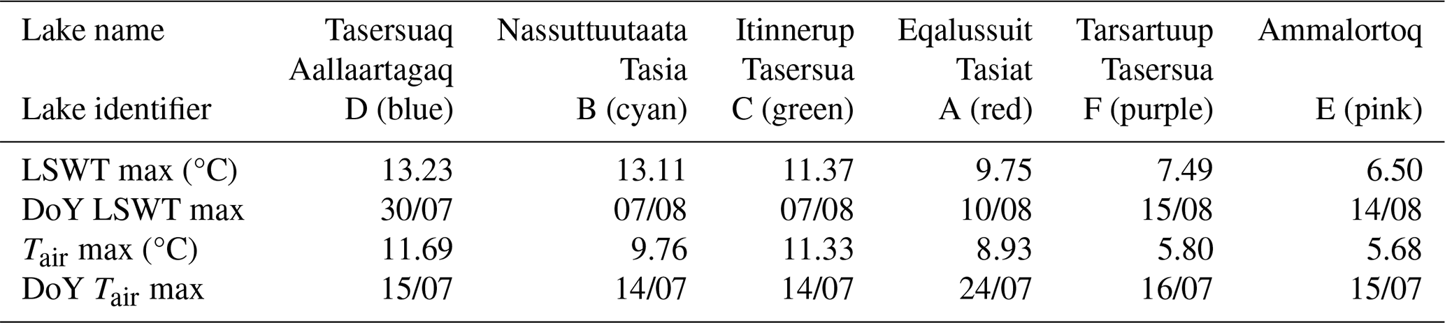
The climatological peak temperatures are in broad correlation with the maximum temperature from Landsat 8 reported in Fig. 4. Each of the six lakes warm, on average, to a temperature greater than 4 °C. The maximum depths estimated for the studied lakes make it plausible they are stratified during periods when LSWT exceeds 4 °C, although potential stratification is only brief in the case of Ammalortoq (Lake E) and Tarsartuup Tasersua (F). As the studied lakes are covered with ice for approximately half of the year, they can most likely be characterized as dimictic. The coolest studied lakes are Ammalortoq (Lake E) and Tarsartuup Tasersua (F), which are not only situated at the highest elevation but are also directly influenced by the GrIS meltwater. Ammalortoq (Lake E) and Tarsartuup Tasersua (F) reach their climatological maximum value of LSWT of 6.5±1.6 and 7.5±1.7 °C on 14 and 15 August, respectively. Between May and the end of August, LSWT in Tarsartuup Tasersua (Lake F) is between 1–2 °C warmer on average than Ammalortoq (Lake E). Ammalortoq (Lake E) is likely colder than Tarsartuup Tasersua (Lake F) due to its smaller size and shallower depth and perhaps due to it being more easily cooled by the meltwater from the GrIS. However, the two lakes have very similar temperatures on average after the end of August, during the cooling period. Tasersuaq Aallaartagaq (Lake D) and Nassuttuutaata Tasia (B) are the warmest lakes with a very similar maximum average LSWT 13.2±1.6 and 13.1±1.6 °C on 30 July and 7 August, respectively, despite being lakes with different characteristics. As reported in Table 3 the four lakes that are not directly connected to the GrIS peak on average above 10 °C. Similar summer maxima have been reported for smaller lakes, not connected to the GrIS, in previous studies (Anderson et al., 2001; Saros et al., 2016).

Table 3 Average maximum LSWT and 2 m air temperature (T_air); lakes are listed in order of decreasing maximum LSWT.

3.3.3 LSWT in relation to T_air and insolation seasonal cycle

T_air and insolation are two very important drivers of LSWT (Woolway et al., 2017). Despite being the coolest lakes among the six, Ammalortoq (Lake E) and Tarsartuup Tasersua (F) receive the highest insolation (Fig. 7b), being the lakes at the lowest latitude, but T_air is the lowest, with the lakes at the highest elevation showing that very likely the insolation will result in a lower temperature (on average), contributing to the melt of the GrIS, which in turn generates a cold water influx into the lake that in turn masks the contribution of the insolation. Tasersuaq Aallaartagaq (Lake D) and Nassuttuutaata Tasia (B) experience very similar maximum temperatures. Tasersuaq Aallaartagaq (Lake D) is likely shallower than Nassuttuutaata Tasia (Lake B). Tasersuaq Aallaartagaq (Lake D) is situated at a lower latitude than Eqalussuit Tasiat (Lake A), Nassuttuutaata Tasia (B), and Itinnerup Tasersua (C), and Fig. 7a shows the warmest seasonal cycle of T_air for Tasersuaq Aallaartagaq (Lake D). Moreover, ERA5-Land indicates higher insolation for Tasersuaq Aallaartagaq (Lake D) than for Nassuttuutaata Tasia (Lake B) (Fig. 7b). Based on depth, T_air, and insolation, we would expect a higher maximum temperature for Tasersuaq Aallaartagaq (Lake D) compared to Nassuttuutaata Tasia (Lake B). The fact that the observed difference is insignificant raises the speculation that the river inflow of Tasersuaq Aallaartagaq (Lake D), fed by a colder proglacial lake, is a significant negative heat flux and that this damps the maximum LSWT.

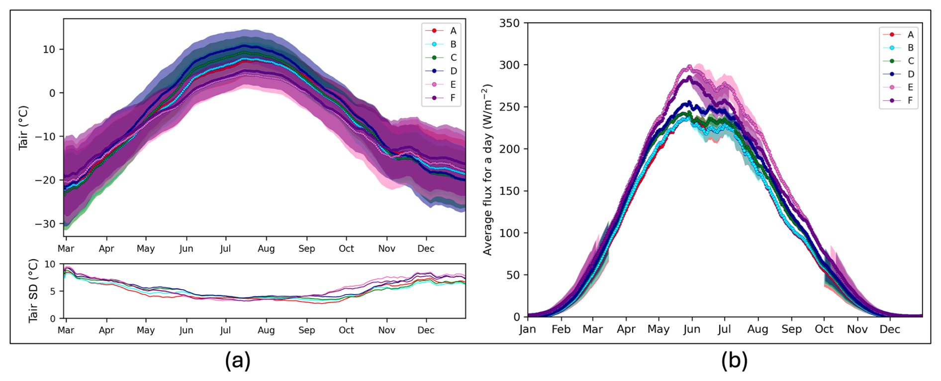
Figure 7 Seasonal cycle (daily means from 1995 to 2020 with a 7 d smoothing window) at the lake centre of T_air (°C) (a) and solar downwelling flux (W m⁻²) from ERA5-Land reanalysis (b). The seasonal cycle is plotted for the six lakes (upper panel), and in the lower plot in panel (a) the values of the standard deviation are reported.

Figure 6a suggests that warmer lakes typically experience an earlier timing of maximum temperature, while the correspondent T_air and insolation maximums happen at a similar timing. Table 3 reports the maximum annual LSWT and T_air and the days of the year of these for all lake centres. The maximum T_air occurs, on average, in mid-July, except for T_air near Eqalussuit Tasiat (Lake A), which occurs about 10 d later. Eqalussuit Tasiat (Lake A) is located at the highest latitude and is closest to the open sea. The maximum LSWT is higher on average and occurs 2 to 4 weeks later than the maximum value of T_air. The longest lag between T_air and LSWT is calculated for the coldest lakes, Ammalortoq (Lake E) and Tarsartuup Tasersua (F), which are connected to the GrIS.

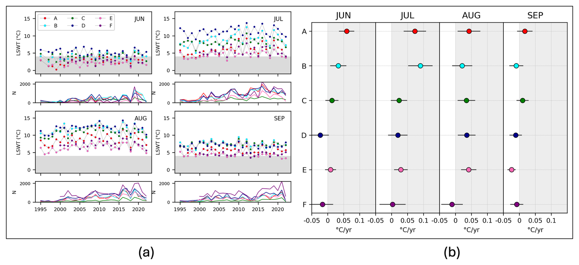
Figure 8 (a) Monthly spatial lake mean time series for the months of June, July, August, and September for the six lakes (upper plot for each of the months) and the number of observations to create the means (lower plot for each of the months). The grey shaded area features temperatures below 4 °C. (b) Trends (linear regression slopes) with the standard uncertainty of the trend (black bar) of the monthly spatial lake mean time series across years for each month and for each lake. The grey shaded area highlights positive values of the trends.

3.3.4 Asymmetry of the LSWT seasonal cycle

Figure 6a (upper plot) shows that all six lakes warm faster and cool more slowly, while the cycles of T_air and insolation are symmetrical. The asymmetry in LSWT over the summer season is due to the effect of ice cover. Upon ice breakup in May, cooler LSWTs are in relatively large disequilibrium with the prevailing T_air and insolation, and the LSWT rapidly increases in response. During the cooling phase, in contrast, the lake has a steadier lagged response to the progressive decrease in T_air and insolation through late summer and autumn. On average, the earliest retrieved LSWTs at the lake centre are a few degrees above 0 °C. This is most likely a sampling effect arising because the first cloud-free observation of the lake centre after ice melt is not immediately after the open water first forms. However, we note that warmer-than-freezing temperatures at the time of ice melt have been reported for lakes in the Tibetan Plateau (Kirillin et al., 2021) and Ontario in Canada (Williams, 1969). In dry, cold atmospheric conditions, solar radiation may be relatively strong and the ice snow-free, enabling a sufficient flux of insolation through the ice to increase the temperature of the water below, even above 4 °C such that there is convective mixing before ice melt. It is uncertain from the satellite observations alone whether such effects are relevant to these lakes.

3.4 Temporal variability in lake mean LSWT

The long-term LSWT variations for the six lakes are shown in Fig. 8 for the months of June, July, August, and September when the lakes are (mostly) ice-free. The warmest months are July and August, when the temperatures among the lakes also differ most. The ranking with respect to temperature tends to be maintained throughout the seasonal cycle.

In June and July, monthly lake mean LSWT in Tasersuaq Aallaartagaq (Lake D) is noticeably higher than the other lakes across the years, while in August and September the LSWTs of Tasersuaq Aallaartagaq (Lake D), Nassuttuutaata Tasia (B), and Itinnerup Tasersua (C) are comparable. Ammalortoq (Lake E) and Tarsartuup Tasersua (F), being connected to the GrIS, do not exhibit a considerable difference in lake mean temperature throughout the years for any of the months. The six time series of monthly lake mean LSWTs in Fig. 8a reveal temporal trends whose values are displayed in Fig. 8b. A total of 12 of the 15 statistically significant trends in Fig. 8b are positive (warming over time). The trends for Eqalussuit Tasiat (Lake A) and Nassuttuutaata Tasia (B) in July are respectively 0.07±0.03 and 0.09±0.04 °C yr⁻¹. Comparing the six lakes, Eqalussuit Tasiat (Lake A) consistently has the highest trends (lake warming at the highest rate) across the months. The highest values for the trend of Eqalussuit Tasiat (Lake A) are in July (0.07±0.03 °C yr⁻¹) and August (0.04±0.03 °C yr⁻¹). This can be related to the fact that Eqalussuit Tasiat (Lake A) is not connected to the GrIS; it is close to the coast and therefore possibly more exposed to meteorological drivers than the other lakes.

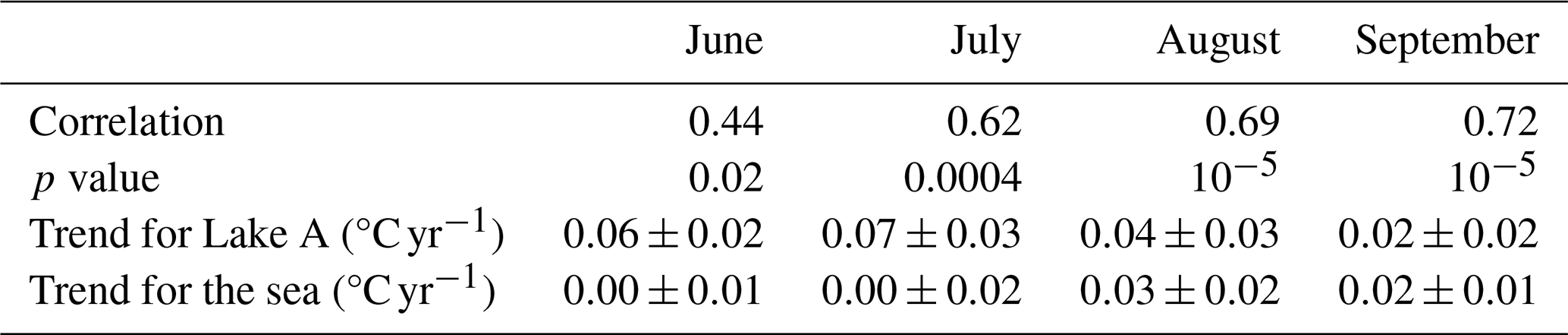
To consider the marine influence on Eqalussuit Tasiat (Lake A), which is close to the coast, SSTs for June to September have been computed from the ESA CCI SST dataset (Merchant et al., 2019), covering a 2° box centred on Eqalussuit Tasiat's latitude immediately to the west. LSWT is 2 °C warmer than the nearby SST during July and August and warmer by less a 1 °C in June and September. The interannual correlation between LSWT and SST is positive and statistically significant for all 4 months. The mean trend across the 4 months is 0.01±0.01 °C yr⁻¹ in the offshore SST and 0.05±0.01 °C yr⁻¹ in the LSWT. Together, the statistics suggest a coupling to the marine climate and an amplified response. The monthly statistics are shown in Table 4. The lakes connected to the GrIS (Tasersuaq Aallaartagaq (Lake D), Ammalortoq (E), and Tarsartuup Tasersua (F)) tend to show smaller interannual trends than the unconnected lakes, although the distinction is not so clear in August. Ammalortoq (Lake E) is overall warming faster than Tarsartuup Tasersua (Lake F). Tasersuaq Aallaartagaq (Lake D) experiences contrasting trends that are negative in June and September and positive in July and August. Speculatively, the overall distinction between Eqalussuit Tasiat (Lake A), Nassuttuutaata Tasia (B), and Itinnerup Tasersua (C) compared to Tasersuaq Aallaartagaq (Lake D), Ammalortoq (E), and Tarsartuup Tasersua (F) may reflect a negative feedback for the connected lakes via the flux of meltwater. However, Tasersuaq Aallaartagaq (Lake D) is connected only via a river, and, speculatively, warming of the meltwater during passage to Tasersuaq Aallaartagaq (Lake D) could act in opposition to this negative feedback, particularly in July and August when the landscape is warmest.

Table 4 Trend comparison between Eqalussuit Tasiat (Lake A) and the closest sea for June, July, August, and September.

3.5 Lake stratification phenology

We estimate lake stratification phenology as the day of the year when the LSWT crosses 3.98 °C. On average, warmer lakes in the study region experience an earlier onset and later breakup of thermal stratification. In turn, the cooler lakes, which are directly connected to the GrIS, experience the latest onset and earliest breakup of stratification (Fig. 9c). Tarsartuup Tasersua (Lake F) on average reaches ∼4 °C on 1 July and Ammalortoq (Lake E) on 7 July, while for the other lakes this happens between 11 and 28 June. Following the warm season, LSWT in Tarsartuup Tasersua (Lake F) cools, on average, below ∼4 °C on 22 September and Ammalortoq (Lake E) on 18 September, while for the other lakes this happens between 1 and 12 October. The time series of the days of the year of onset and breakup of stratification follow an asymmetric cycle: the breakup date is relatively stable across the six lakes, while the onset tends to occur substantially earlier in the year during the study period, other than for Tarsartuup Tasersua (F) (Fig. 9a). The largest rates of change in stratification onset are $-\mathrm{0.5}\pm \mathrm{0.2}$ d yr⁻¹ for Eqalussuit Tasiat (Lake A) and Nassuttuutaata Tasia (B) (Fig. 9b). The breakup of stratification only occurs later in the year for Eqalussuit Tasiat (Lake A) (0.2±0.2 d yr⁻¹). The warm stratified season is lengthening for the three lakes that are not connected to the GrIS (Fig. 9), while this is less clear for the connected lakes given the trend uncertainties.

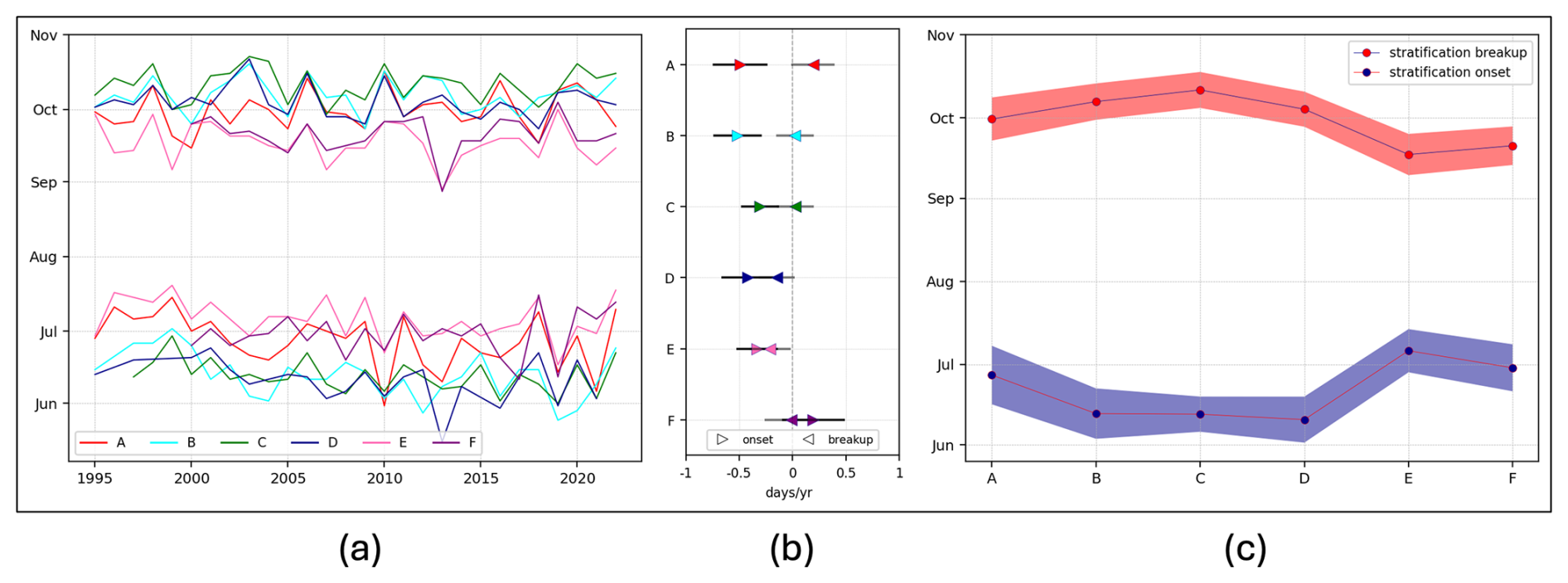
Figure 9 (a) Time series of the stratification onset and breakup timing (day of the year) for the six lakes. (b) Trends (linear regression slopes) with the standard uncertainty (black bar) of the stratification onset and breakup timing (days per year) for the six lakes. (c) Average day of the year for the stratification onset and breakup, where the shaded area represents 1 standard deviation from the mean, expressing the variability of the thermal stratification phenology across the years.

3.6 Factors influencing the variability in LSWT and stratification phenology

T_air is typically considered the most important atmospheric driver of LSWT (Edinger et al., 1968), but their relationships differ across seasons. Here, we calculated the correlation (Spearman) between T_air and LSWT anomalies across the studied lakes (Fig. 10) in time. Figure 10a and 10b show the interannual correlation between the June and August (respectively) LSWT anomaly and the T_air anomalies of each of the months of the year. For all six lakes, LSWT anomalies in June are best correlated with T_air anomalies in May (Fig. 10a). This seems to arise because the lake ice-off date strongly influences the June LSWT anomaly. Earlier ice-off results in a rapid initial rise of LSWT during summer, thus influencing the June LSWT. Warmer T_air in May can lead to earlier ice-off. This interpretation is supported by the observation that the stratification onset date is better correlated with the May T_air anomaly (mean of correlation coefficient across the six lakes: 0.7±0.1) than with that of June (0.5±0.1), despite stratification onset usually occurring during June. In contrast, LSWT anomalies in August (Fig. 10b) are most significantly correlated with the August T_air anomalies. During this time the lakes are likely thermally stratified and the volume of water interacting with the atmosphere is relatively small. The exceptions to the high correlation for August are Ammalortoq (Lake E) and Tarsartuup Tasersua (F) that directly receive GrIS meltwater. Since warm T_air is expected to increase meltwater discharge (but not, for an ice-marginal lake, meltwater temperature), it appears that LSWT–T_air correlation for August is in these cases suppressed by a negative feedback via enhanced cooling by water influx from the GrIS.

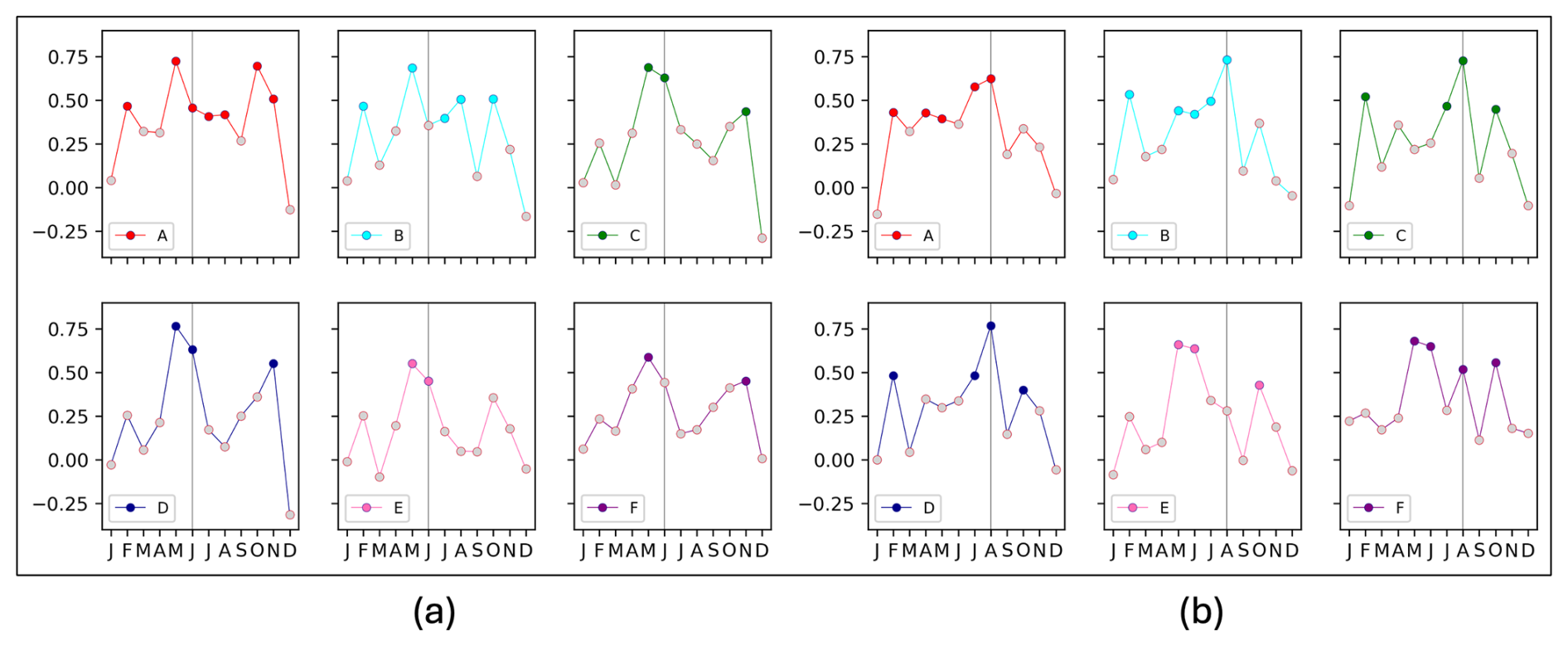
Figure 10 Correlations (Spearman) between LSWT anomalies for the month of June (a) and August (b) and the T_air anomalies from ERA5-Land for all the months in the year. The grey circles indicate a p value greater than 0.05.

The most important driver of the stratification phenology is air temperature (Woolway et al., 2021). The correlation between stratification phenology and T_air is found to be relevant and significant only for the onset, while for the breakup only mild correlations appear for the lakes connected to the GrIS and Eqalussuit Tasiat (Lake A). For Tasersuaq Aallaartagaq (Lake D), which is connected to the GrIS through a long stream, the correlations with T_air are not significant, indicating that the changes in the stratification timing are driven by other factors. The highest correlations are found for stratification onset for the lakes directly connected to the GrIS (Ammalortoq (Lake E), Tarsartuup Tasersua (F), and Eqalussuit Tasiat (Lake A)). Correlations with the shortwave solar radiation anomalies have been investigated using the surface solar irradiance values from ERA5-Land and using the ESA CCI Clouds observations (Stengel et al., 2020). No significant correlation has been found for any of the lakes with either dataset.

4 Discussion

4.1 Spatial thermal characteristics of lakes in the region with high-resolution sensor

High-resolution thermal remote sensing allowed characterizing the lakes in the region spatially only since currently high-resolution sensors have low revisiting time. Analysing data from 138 lakes observable in Landsat 8 imagery, we observed a wide spectrum of maximum LSWTs varying from 5 to 20 °C, alongside varying surface albedo values spanning 0.03 to 0.14. Notably, high-albedo lakes, often connected directly to the GrIS or indirectly through river systems, tend to exhibit cooler temperatures. This cooling effect is attributed to their enhanced reflectivity, which reduces solar absorption, coupled with the influence of cold glacial meltwater inflows. Conversely, smaller and typically shallower lakes with lower albedo tend to absorb more solar radiation and consequently reach warmer temperatures (Read and Rose, 2013; Heiskanen et al., 2015). These findings underscore the complex relationship between lake morphology, solar radiation dynamics, and climatic influences, essential for understanding the response of these ecosystems to climate change. The six lakes that have been selected specifically for this study are representative of the lakes in the region exhibiting different albedos, temperatures, and elevations. The only limitation to the variety of lakes was the size since meteorological satellites used to create the ESA CCI Lakes dataset have a spatial resolution of about 1 km.

4.2 Seasonal trends in LSWT and LIC

Meteorological sensors provided critical time series of LSWT and LIC observations that enabled us to uncover nuanced insights into the thermal dynamics of these water bodies. These six studied lakes had contrasting elevation and proximity to the GrIS, as well as to the sea. Seasonally, these lakes exhibit significant variability in ice cover, typically remaining ice-free from June through to November, although the exact timing of complete ice reformation is affected by some observational uncertainty. This seasonal pattern, notably asynchronous with the solar insolation cycle, underscores the complex interplay of climatic factors influencing lake dynamics. The detailed examination of these lakes reveals distinct thermal dynamics and responses to environmental stimuli. Lakes not directly connected to the GrIS typically reach peak temperatures ranging from 9 to 14 °C during the summer months, exceeding average air temperatures due to direct solar heating. In contrast, ice-marginal lakes exhibit cooler peak temperatures around 7 °C, a phenomenon not fully explained by their elevated albedo alone. The influx of cold meltwater from nearby glaciers likely plays an important role, impacting the thermal balance and seasonal variations of these water bodies. Analysing the seasonal cycle, we found that the warm stratified season of the studied lakes typically spans from mid-June to early October, though it is slightly shorter for cooler ice-marginal lakes, and that all six lakes warm faster and cool more slowly due to the effect of the ice cover. In contrast, the forcing cycles of T_air and insolation are relatively symmetrical. When the ice breaks up in May, the cooler LSWTs are significantly out of balance with the prevailing T_air and solar radiation, leading to a swift rise in LSWT. In contrast, during the cooling phase, the lake reacts more slowly, with a lagged response to the gradual decline in T_air and solar radiation throughout late summer and autumn.

4.3 Temporal variability in LSWT

The observed interannual variability in these processes highlights the sensitivity of West Greenland lakes to fluctuations in atmospheric conditions, emphasizing their role as indicator of broader climatic trends in the region. Over the months of June to September, LSWT trends varied from insignificantly negative to warming trends of 0.5–1 °C decade⁻¹ across different lakes with clear differences for ice-marginal lakes, coastal lakes, and inland lakes. Stratification onset appears to be advancing by approximately 5–8 d decade⁻¹, while the end of stratification shows more stability over time, consistent with studies from other regions worldwide (Woolway et al., 2021). Our findings suggest that ice-marginal lakes may increasingly interact with the dynamics of the GrIS margin, potentially becoming more important in the future (Mallalieu et al., 2021; Carrivick et al., 2022). Changes in water temperature and stratification phenology substantially impact light availability, nutrient cycling, and oxygen levels crucial for lake ecosystems (Woolway et al., 2021). Surface water temperature serves as a “sentinel” of climate change, integrating various climatic and in-lake drivers that influence the lake's surface energy budget (Woolway et al., 2021; Schneider and Hook, 2010). Understanding these dynamics is crucial for assessing the resilience of West Greenland's lakes to ongoing environmental changes and their implications for ecosystem health and function.

4.4 Influence of air temperature and insolation on LSWT and lake stratification

Air temperature conditions leading up to the ice-free season, particularly in May, emerge as a pivotal factor influencing both stratification onset and the timing of ice-off events. The onset of stratification correlates closely with air temperature in the preceding month, influencing the rate of lake ice melt. Our study found no significant influence of insolation on this process. Warmer temperatures during the period leading to the ice-free season accelerate the melting of lake ice, influencing stratification dynamics and subsequent thermal regimes. The influx of cold meltwater from nearby glaciers likely acts as a significant cooling mechanism, influencing the thermal balance and seasonal variability of these water bodies. The high albedo of ice-marginal lakes suggests substantial influx of mass and meltwater from the GrIS. This meltwater introduces a negative heat flux that correlates with August air temperatures, affecting glacial melting dynamics. The lack of correlation with August air temperature for ice-marginal lakes arises from competing mechanisms, notably warming from solar radiation and cooling from meltwater influx associated with warmer summer air temperatures, complicating the LSWT response to climate change.

4.5 Implications for LSWT and LIC studies in Greenland and the Arctic

Observations of the temperature of proglacial lakes in this landscape are sparse. It has been assumed in some mass balance models of glaciers terminating in lakes that the lakes do not warm to more than 1 °C (Truffer and Motyka, 2016; Chernos et al., 2016), a notion contradicted by the remotely sensed data analysed in this study. This discrepancy underscores the necessity of leveraging remote sensing to complement sparse in situ data in regions like West Greenland. However, only large lakes (of area at least 3 km²) can be observed with good temporal resolution by meteorological satellites (used for ESA CCI Lakes dataset), which offer a sufficiently long time series to detect climatic signals and well-characterized uncertainty and stability. For smaller lakes, higher-spatial-resolution satellites, such as Landsat 8, can offer observations at a finer spatial resolution (100 m), but a much longer revisiting time is often insufficient for a good description of the temporal variations. An example is the use of the high-spatial-resolution sensor ASTER to characterize the thermal behaviour of lakes in Arctic Sweden where the measurements considered were very sparse in time (Dye et al., 2021). These are current limitations of remote sensing data, which will be partly addressed with improvements in spatial and temporal resolution such as those provided by the satellites for thermal remote sensing such as TRISHNA (Lagouarde et al., 2018) to be launched after 2025. Furthermore, a lake–glacier interaction mechanism could be better investigated through new fieldwork. Collecting ground-truth data would be very useful to more precisely quantify the interactions between lakes and the ice sheet and to unravel the complex thermal structure at various depths of these lakes and how it varies in space and time. Such approaches are essential for elucidating the complex relationships between climatic variables, ice dynamics, and lake behaviours, providing critical insights into ecosystem responses to climate change in such a key region for local and global climate.

5 Conclusions

Lakes are important features of West Greenland's seasonally ice-free landscape, their biogeophysical interactions in summer being in part determined by their energy budget and the LSWT they reach. In this study, we presented new, long-term, and consistent LSWT information for lakes across this landscape using satellite data.

A broader analysis across the region to characterize thermally the lakes in space was achieved with high-spatial-resolution data from Landsat 8. Investigations of specific dynamics were conducted on six lakes in West Greenland using high-temporal-resolution meteorological sensor data, the ESA CCI Lakes data. The six lakes are located at contrasting elevations and proximity to the GrIS and to the coast, allowing us to unveil their long-term thermal behaviour (seasonal climatology and interannual variability) for the first time and to attempt to disentangle the complex interaction between lake morphology, solar radiation dynamics, and climatic influences as well as the influence of atmospheric variables on the lake dynamics in detail and in a consistent manner. Contrary to some mass balance models of glaciers terminating in lakes, we found that these lakes warm to much more than 1 °C, reaching on average a water temperature between 6.6–7.5 °C. The lakes not connected to the ice sheet reach an average surface water temperature of more than 13 °C.

The most important atmospheric driver is air temperature. However, the ice sheet significantly impacts the thermal behaviour of the lakes, frequently overshadowing the atmospheric signatures. For example, no correlation is found in summer between LSWT anomalies and T_air: only for the ice-marginal lakes, indicating a mitigation of T_air impact on the lakes by an enhanced cooling of water influx from the GrIS. The vicinity of the coast also influences lake thermal state. The lake temperature is influenced by the marine climate, and a comparison with nearby SST shows that the lake amplifies the response, consistently exhibiting the largest trend in temperatures (increase at a rate of more than half a degree per decade) and in stratification onset (half a day per year earlier) and breakup (a quarter of a day later per year) timing among the six lakes.

Advancements in satellite remote sensing have enhanced the radiometric, spatial, and temporal quality of observations, enabling long-term thermal characterization of lakes covering large areas in a consistent way, as demonstrated in this study. Satellite data are especially crucial in remote and data-sparse regions such as Greenland. However, current Earth observation missions often face trade-offs between spatial and temporal resolution. These limitations are expected to be addressed by upcoming missions such as TRISHNA, which aim to provide high-resolution thermal and optical data with improved revisit times. Complementary in situ data collection remains critical for quantifying the hydrological and cryospheric interactions, particularly those between proglacial lakes and the Greenland Ice Sheet.