Trace metal distributions in the transition zone from the Greenland Ice Sheet to the surface water in Kangerlussuaq fjord (67° N)

Glacial rock flour (GRF), an ultra-fine sediment formed beneath glaciers, contains high concentrations of silicate and trace metals, including iron (Fe) and manganese (Mn). In Greenland, meltwater discharge transports approximately 1.28 Gt of suspended sediments annually into the oceans, significantly influencing trace metal concentrations and marine biogeochemical cycles. This study investigates the spatial distribution of trace metals, nutrients, and suspended sediment concentration (SSC) from the Russell Glacier at the Greenland Ice Sheet, through the Akuliarusiarsuup Kuua meltwater and into the Kangerlussuaq fjord in western Greenland. Dissolved trace metals were relatively high in the river with low-salinity surface waters in the fjord, showing that the fjord acts as an important source of trace metals for the marine environment. However, trace metal concentrations, particularly Fe and zinc (Zn), exhibited significant non-linear decreases beyond salinity levels of 14, underscoring the complex processes affecting trace metal supply from rivers to fjords and coastal waters. In contrast, silicate concentrations increased in river water due to weathering of GRF and decreased gradually in the inner fjord due to mixing with surface water. Uranium (U) and molybdenum (Mo) were undetectable along the river but increased in the fjord, indicating that these elements primarily originate from the ocean. These findings highlight the complex interplay of physical, chemical, and biological processes regulating trace metal and nutrient dynamics in glacier-influenced fjord systems, with implications for primary productivity and carbon cycling in polar oceans.

1 Introduction

Nearly all glaciers in Greenland have been thinning or retreating in the past few decades, and the Greenland Ice Sheet (GrIS) has experienced an acceleration in calving events since 1985 (Chen et al., 2006; Zeising et al., 2024; Greene et al., 2024). Due to this mass loss driven by increased surface melting and enhanced discharge from outlet glaciers (IMBIE Team, 2020), the GrIS is one of the largest contributors to contemporary sea level rise globally (Bamber et al., 2019), adding an average of 0.77 mm yr⁻¹ (Clark et al., 2015), that is 21 % of the global mean since 1993 (WCRP, 2018). Half of the ice mass loss in polar zones over the last decades resulting from warming is caused by ice-sheet discharge through the marine-terminating glaciers (Shepherd and Wingham, 2007; Slater et al., 2021). Climate models suggest that continued ice loss in Greenland will accelerate (Khan et al., 2022), leading to an increased contribution of global mean sea level rise from the GrIS by 2100 (Goelzer et al., 2020; Edwards et al., 2021; Aschwanden and Brinkerhoff, 2022; Paxman et al., 2024).

The debris from glacial erosion, which contributes to approximately 7 %–9 % of the global sediment flux to the sea (Overeem et al., 2017), contains fine sediments which remain in suspension and are transported into the coastal ocean waters. In Greenland particularly, meltwater transports ∼0.6–1.3 Gt of suspended sediments into the oceans every year (Hasholt et al., 2006; Overeem et al., 2017; Hawkings et al., 2017) where fine particles dominate the sediment. These ultra-fine sediments originating beneath the GrIS from the erosion of the bedrock by glacial movement are referred to as glacial rock flour (GRF). The heavy physical erosion makes the GRF relatively less chemically mature compared to more weathered sediments, and its mineralogical composition is therefore very similar to its source rocks. The composition of GRF varies depending on the bedrock source, but in southwest Greenland a common suite of present minerals is quartz, feldspars, phyllosilicates, and amphiboles. GRF is also a felsic silicate mineral which contains a suite of trace metals, e.g. iron.

While it is established that glacial discharge and sediments from glacial erosion are primarily transported through rivers and into the fjords, the mechanisms governing the transition of trace metal inputs, particularly from glaciers and glacial rock flour, into marine systems remain unclear. Trace metals, such as iron, are critical micronutrients for phytoplankton growth and biological processes, thereby playing an essential role in the global carbon cycle. For example, iron is a vital component in photosynthetic proteins involved in the electron transport chain and redox reactions within the photosystem II apparatus (Strzepek et al., 2012; Raven et al., 1999). In high-nutrient, low-chlorophyll (HNLC) regions like the Southern Ocean and parts of the North Pacific and North Atlantic, trace metal availability is a limiting factor for primary productivity and subsequent carbon export (Boyd and Ellwood, 2010). Silicon limitation of diatom production is also present in this region and in other parts of the Arctic (Krause et al., 2018, 2019; Ng et al., 2024). Hence, alongside macronutrients such as phosphate and nitrate, levels of silicate and trace metals regulate oceanic biological production in this region.

Other iron sources such as aeolian iron or dust support primary production in regions of the northeast Atlantic (Blain et al., 2004). However, previous studies have found that aeolian sources are not sufficient to support primary production in the North Atlantic during spring and summer (Moore et al., 2006). Other studies have also found that regions of the North Atlantic become iron limited in the summer (Nielsdóttir et al., 2009; Ryan-Keogh et al., 2013; Browning and Moore, 2023). Greenland glacial meltwater has been identified as a significant source of bioavailable iron (Hawkings et al., 2014) and silica (Hawkings et al., 2017), with an estimated annual flux of dissolved and potentially bioavailable particulate iron to the North Atlantic Ocean of approximately 0.3 Tg (Bhatia et al., 2013). Understanding the fluxes and transformations of these trace metals from glacial systems to oceanic environments is crucial for predicting their contribution to marine biogeochemical cycles under ongoing climate change. However, field data and a more complete understanding of processes acting on the dissolved suspended material from the glaciers through transitioning rivers and into the fjords are lacking, particularly for a wider range of trace metals and macronutrients like nitrate, silicate, and phosphate.

Furthermore, GRF is considered as a potential means of action for marine carbon dioxide removal (mCDR). Weathering of GRF supplies the ocean with macronutrients and trace metals, supporting phytoplankton growth (Bendtsen et al., 2024). Additionally, GRF has been shown to increase the effects of enhanced rock weathering on land, due to its high silicate content (Gunnarsen et al., 2023; Dietzen and Rosing, 2023). Its dissolution in seawater supplies essential micronutrients, e.g. trace metals, like iron and manganese, which can alleviate nutrient limitations and promote carbon sequestration. However, the impact from many different processes, e.g. adsorption, flocculation, and scavenging, affects the distribution of GRF. Therefore, this study also describes the distribution of GRF in its natural environment, motivated by its potential future usage as a source for mCDR.

In this study, we investigate the distributions of trace metals and macronutrients in the transition zone from the Russell Glacier at the Greenland Ice Sheet, through the Akuliarusiarsuup Kuua meltwater, and into the inner part of Kangerlussuaq Fjord. Meltwater and seawater samples were analysed for trace metals, nutrients, and other environmental variables, e.g. salinity and suspended sediment. Finally, the role of internal sinks, e.g. adsorption and biological uptake, for the transport of GRF-related trace metals to the open ocean is discussed.

2 Methods

2.1 Study area

Samples were collected during the Glacial Rock Flour in the Sea (GROFS1) field campaign, from 20 June to 6 July 2023. Sampling was carried out in the inner part of the Kangerlussuaq fjord located in west Greenland (∼67° N) and along the meltwater river (Akuliarusiarsuup Kuua, alternatively Watson River) that enters the bottom of the fjord (Fig. 1). The river originates at Russell Glacier – an ice tongue from the GrIS. Water was sampled at 35 stations that covered the transition zone from Russell Glacier, along the Akuliarusiarsuup Kuua, and into and along the inner part of Kangerlussuaq fjord. The river receives runoff from three major glacier tongues along its passage from Russell Glacier and towards the fjord (Hasholt et al., 2018). The town and airport of Kangerlussuaq are located at the outlet of the river that enters the fjord via an ∼10 km long river delta. The inner fjord covered the area from the river delta and about half-way into the inner basin of Kangerlussuaq fjord. Kangerlussuaq fjord is a 100 km long fjord and is separated into a deep inner and relatively shallow outer basin. The two basins are separated by a narrow and shallow strait. The inner basin is about 80 km long and in general deeper than 200 m with a maximum depth of ∼275 m (Nielsen et al., 2010).

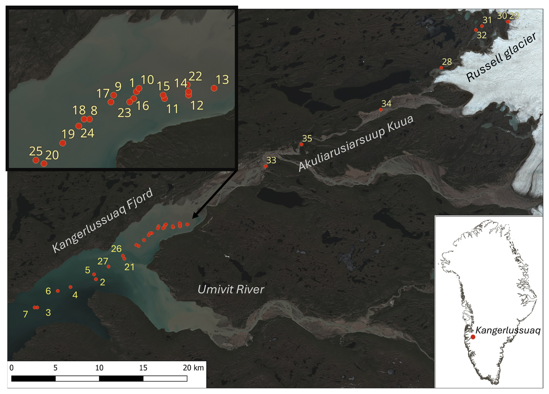
Figure 1 Study area in Kangerlussuaq fjord and stations for water sampling in the fjord and in the river towards the GrIS. Station numbers are shown in yellow, and the location of the fjord system is indicated on the map of Greenland. The Sentinel-2 satellite image is from 2 July 2023.

The inner basin receives freshwater from the Akuliarusiarsuup Kuua and Umivit river. The Akuliarusiarsuup Kuua is passing below the Kangerlussuaq bridge (alternatively Jack T. Perry Memorial Bridge) at Kangerlussuaq town, and the annual discharge has been observed to vary between 3.8–11.2 km³ in the period 2006–2017 (van As et al., 2018). Runoff starts in spring and obtains peak values of ∼2000 m³ s⁻¹ in July. In 2023 the sea ice was reported to break up in early June, and the spring was relatively dry compared to the previous 10 years (Fig. 2). Hence, runoff in early June was relatively modest, and the estimated accumulated runoff from the river by the end of June was 0.2 km³ (van As, 2022). However, a relatively large river transport was visually observed at the outlet at Kangerlussuaq town during the entire field campaign. The discharge from the Umivit river has been estimated to be ∼70 % larger than the discharge from the Akuliarusiarsuup Kuua (Monteban et al., 2020). The area off the fjord arm with the Umivit river outlet that connects to the main fjord was located at a distance of ∼50 km from the glacier, i.e. ∼10 km from the Akuliarusiarsuup Kuua outlet (Fig. 1).

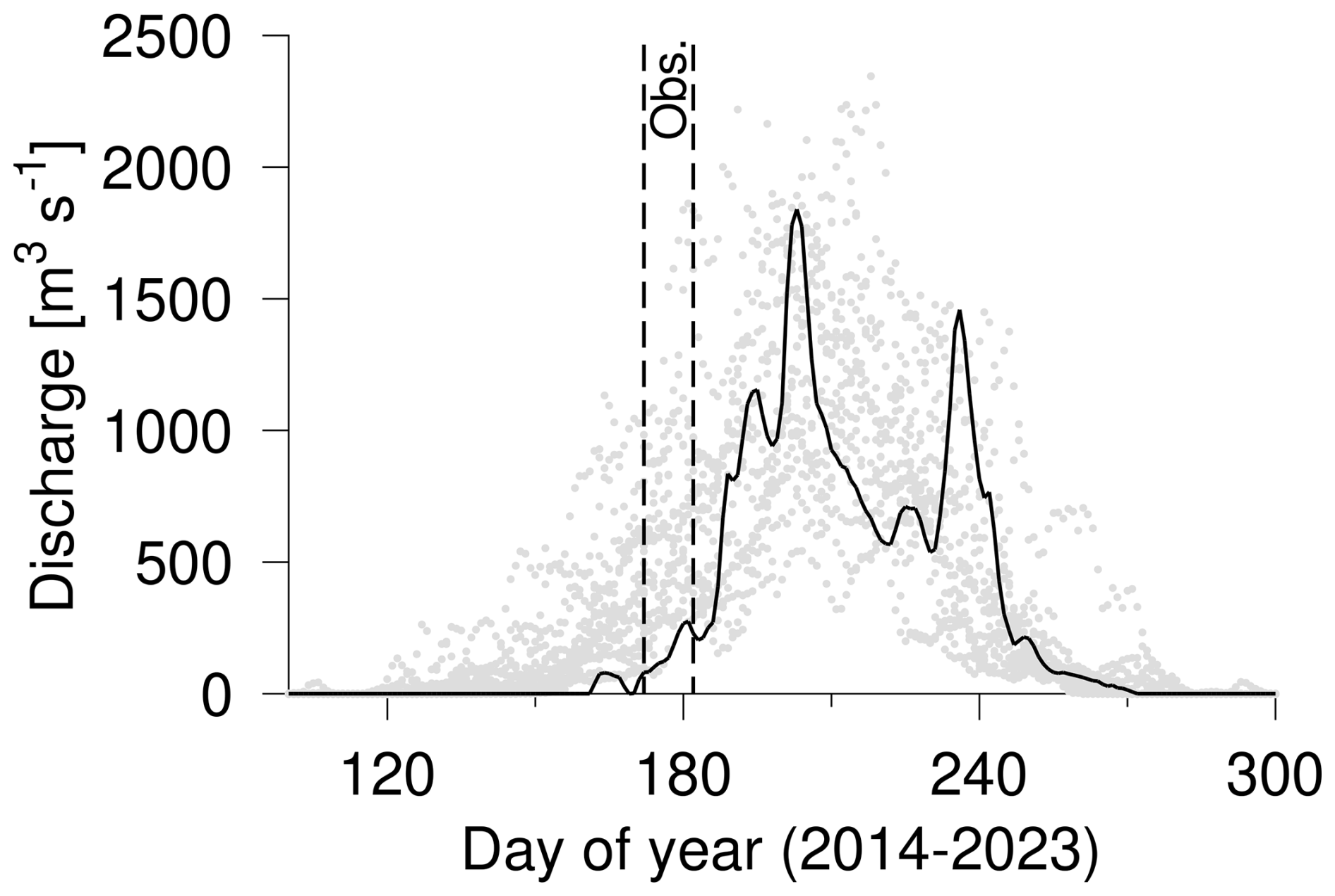
Figure 2 Discharge from the Akuliarusiarsuup Kuua (van As, 2022) in the period 2014–2022 (light grey bullets) and in 2023 (black line). The period of the field campaign is indicated (dashed lines). The river data are a reanalysis product (van As et al., 2018).

A total of 27 samples were collected from stations within the fjord. In addition, 8 meltwater river samples were collected: 6 from stations along the river and 2 from stations located less than 200 m from the glacier (Table A1). The total transect from the glacier to the outermost station in the fjord was ∼65 km. A detailed synoptic transect was made from a station in the innermost part of the fjord and within a distance of ∼5 km from the river delta and ∼6 km into the fjord. This transect was made within 2 h, vertical profiles were made at the end stations (sts. 13 and 20), and surface samples (0–1 m depth) were collected at stations in between. The transect covered an area with a visible change of suspended material from the river plume, and the synoptic transect ended in the middle of the fjord and off the Umivit fjord arm.

2.2 Temperature, salinity, and freshwater content

Measurements of conductivity (C), temperature (T) and pressure, i.e. ∼ depth (D), were made with a loose-tethered free-fall Rockland Scientific International (RSI) VMP-250 microstructure vertical profiler in the upper ∼150 m. The profiler was equipped with a conductivity, temperature, and pressure sensor (JFE Advantech) that operated at 16 Hz. In addition, an underway CTD (conductivity, temperature, depth) probe (Ocean Science, Sea-Bird CTD) was applied at stations where water samples only were made in the upper 10 m (sts. 23–26). Measurements from the VMP CTD and the underway CTD (UCTD) were in accordance, and a comparison at 40 m depth showed a difference of less than 0.1 °C and 0.1 g kg⁻¹ for temperature and salinity, respectively.

Temperature, salinity, and density are reported as conservative temperature (Θ), absolute salinity (S_A), and potential density anomaly (σ_Θ), respectively (IOC et al., 2010). The correction factor for absolute salinity is not well described in coastal waters and fjords around Greenland (Bendtsen et al., 2021) and was therefore set to zero (i.e. δS_A=0). Temperature and salinity samples were binned in 0.5 m intervals from a depth of 0.5 m.

In addition to surface salinity, the freshwater content (F_w) of the upper part of the water column can be applied for analysing the impact from runoff. The freshwater fraction represents the amount of freshwater needed to dilute a water column with a certain reference salinity and of a given depth to obtain the observed salinity. Thus, the freshwater fraction is an integrated measure of the amount of freshwater in the upper layer. Hence, it represents an integrated impact from freshwater sources (e.g. runoff, precipitation, and sea ice melt) over a time period and is therefore not so sensitive to temporal or spatial variation of the surface salinity (Bendtsen et al., 2014). The freshwater content was related to a reference salinity (S₀) of 24.2 g kg⁻¹, representative of the salinity at the bottom of the surface layer (D=15 m) and calculated as

$$F_{\mathrm{w}}=\underset{-D}{\overset{\mathrm{0}}{\int }}{\displaystyle \frac{S_{\mathrm{0}}-S}{S_{\mathrm{0}}}}\mathrm{d}z.$$

The integral is made along the vertical axis (z), and F_w was calculated for each station.

The near-surface salinity (0.5–1 m) at stations along the synoptic transect between stations 13–20 were interpolated between salinities at the end stations, i.e. st. 13 (S_A=6.51 g kg⁻¹) and st. 20 (6.62 g kg⁻¹). Thus, surface salinity showed a minor change along the transect (Fig. 3c). Similarly, the freshwater content was interpolated along the transect between the corresponding values of F_w=2.90 m (st. 13) and 2.38 m (st. 20). The change in F_w of ∼0.5 m reflected that the depth of the surface plume decreased along the transect into the fjord (Fig. 3b, Table A1).

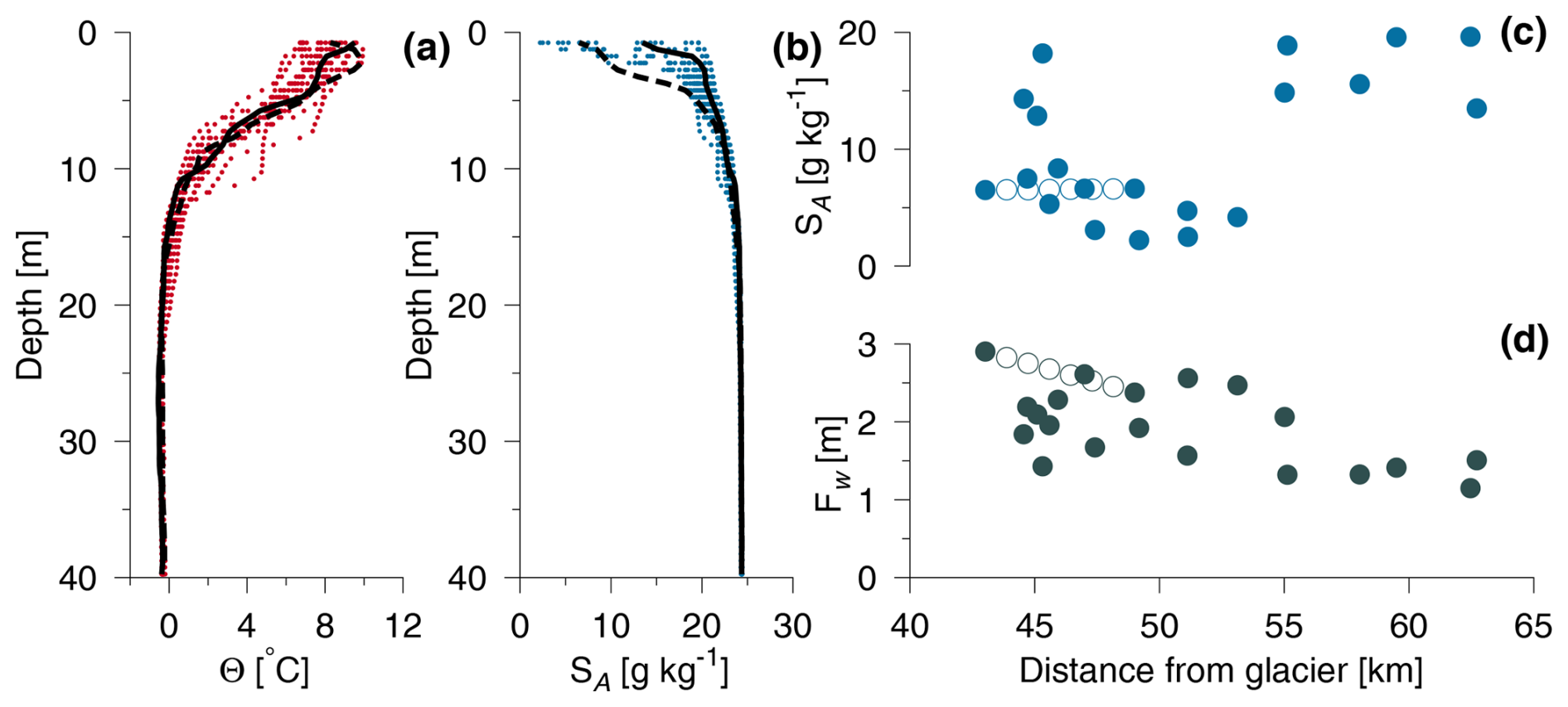
Figure 3 (a) Conservative temperature (red, Θ) and (b) absolute salinity (blue, S_A) measured in the inner part of Kangerlussuaq (sts. 1–27). Stations near the Akuliarusiarsuup Kuua outlet and the furthest distance from the river are shown with dashed and full lines, respectively. (c) Surface salinity (0.5–1 m) and (d) freshwater content (F_w) from stations in the fjord. Interpolated salinity and freshwater content at the synoptic transect between stations 13–20 are marked by hollow circles.

2.3 Dissolved trace metals

Trace metal samples were collected at 28 stations at the surface, with trace-metal-clean low-density polyethylene (LDPE) bottles. Samples were collected from undisturbed water in the fjord and in the river. One station (st. 33) was located beside a bridge at the entrance of the river delta and before the discharge from the small town of Kangerlussuaq. Samples in the river were collected facing the current to avoid contamination. All equipment used to sample the concentration of trace metals in the water was prepared following the GEOTRACES protocol (Cutter et al., 2010). Briefly, LDPE bottles were washed in Decon for 2 weeks before being placed in an acid bath (HCl 6 M) for an additional 4 weeks. All bottles were then rinsed three times with ultrapure Milli-Q water and triple bagged for transportation. To measure dissolved concentrations, aliquots were syringe-filtered through acid-washed Pall Acropak Supor capsule filters (0.2 µm). Prior to analysis, the samples were acidified to 2 % HNO₃ and 0.5 % HCl ($v/v$). The samples were analysed by inductively coupled plasma mass spectrometry (ICP-MS) (7850x, Agilent Technologies) with yttrium as the internal standard at the Sustain Lab (Technical University of Denmark). The instrument was equipped with platinum-tipped skimmer and sample cones, a double-pass Scott spray chamber operated at 2 °C, and a MicroMist nebulizer. Elements analysed in helium (He) collision mode were with a He flow of 5 mL min⁻¹.

Based on repeated measurement of certified in-house standards (SCP Science EnviroMAT), the relative standard deviation (RSD) of the measurements was calculated. Furthermore, each injection of the sample was measured three times, in order to estimate the RSD of each individual measurement. The method detection limit (MDL) was calculated from the calibration curve. To enhance the measurement precision (lowest point 0.05 mg L⁻¹), the axial view setting was used for measurement of concentrations <1 mg L⁻¹ and radial view for concentrations >1 mg L⁻¹. The seawater samples were diluted 10 times to decrease the salinity, and the calibration curves and standards were prepared in a corresponding matrix solution made with artificial pure NaCl. The background levels from laboratory blanks were analysed and included in the corrections and detection limit calculations. Quantification limits for each element are listed in Table 1. Processing of the data was carried out in the Syngistic™ for ICP software v. 2.0 from Perkin Elmer.

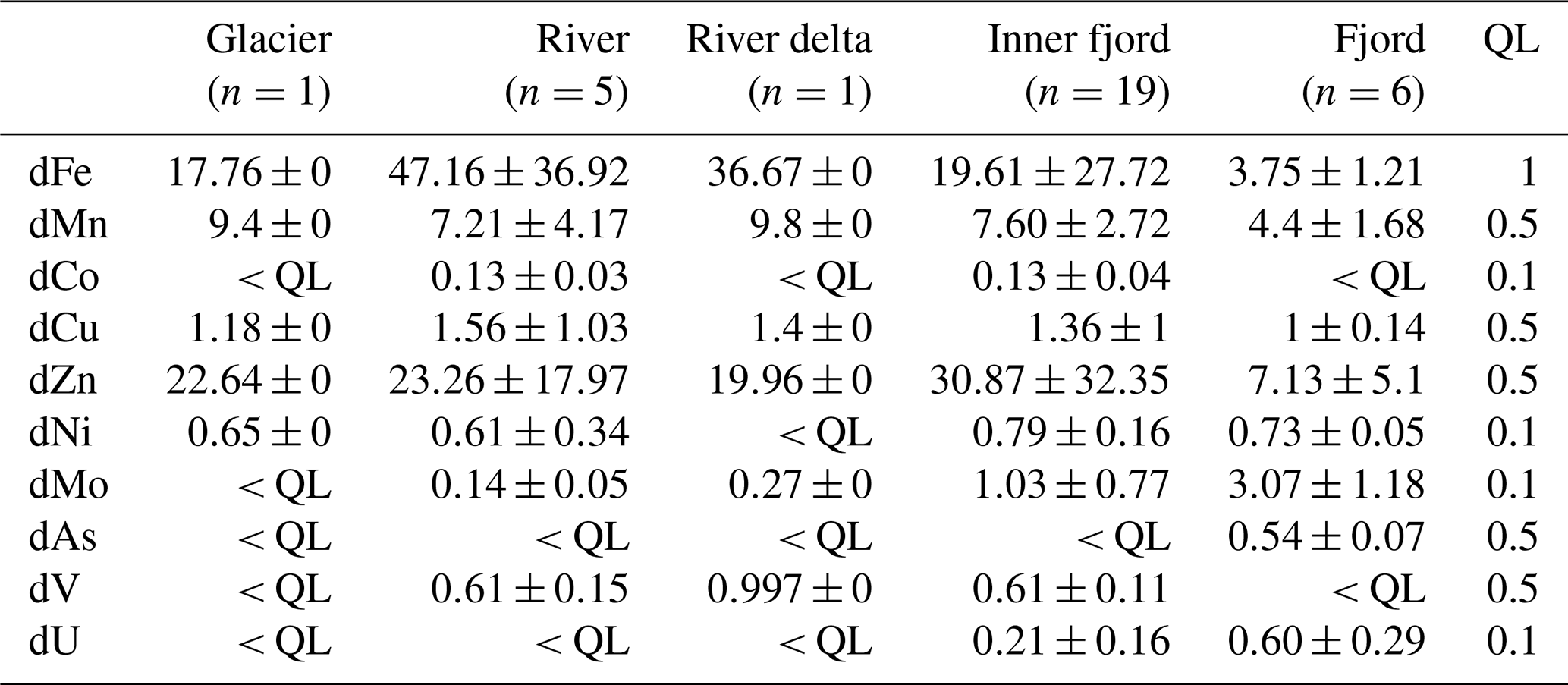
Table 1 Mean and standard error for concentrations (µg L⁻¹) of dissolved trace metals. The transect is divided into five distinct areas: glacier, river, river delta, inner fjord (low salinity <13), and fjord (high salinity). Dissolved trace metals included are iron (Fe), manganese (Mn), cobalt (Co), copper (Cu), zinc (Zn), nickel (Ni), molybdenum (Mo), arsenic (As), vanadium (V), and uranium (U). Values below the quantification limit (QL) are shown as “< QL”, and the QL for each element (µg L⁻¹) is shown, respectively. A table including all trace metal samples is included in Table A2 in Appendix A, and the corresponding instrument uncertainties are shown in Table S1 in the Supplement.

2.4 Nutrients and suspended sediment

Water samples for nutrients and suspended sediment concentration (SSC) were collected using a 5 L Niskin bottle operated by a messenger. Water samples were collected at standard depths in the upper 40 m. Samples for nutrients were filtered through a syringe filter (Filtropur S, polyethersulfone (PES) membrane, pore size 0.2 µm) and immediately placed in a cool box (<0 °C) and stored at −20 °C on land within 6 h. While we acknowledge that freezing turbid samples can affect silicate concentration measurements (MacDonald and McLaughlin, 1982; Macdonald et al., 1986), filtering through a 0.2 µm filter minimizes turbidity-related loss of molybdate-reactive silicate. The samples were analysed for nitrite, nitrate, ammonia, phosphate, and silicate by wet-chemistry methods (Grasshoff, 1983) with detection limits of 0.04, 0.1, 0.3, 0.06, and 0.2 µM, respectively (Danish Centre for Environment and Energy (DCE), Aarhus University, Denmark). The suspended sediment concentration (SSC) was determined from 1–5 L water samples filtered through a 200 µm mesh on site and 0.3 µm glass fibre filters (Advantec GF-75, ø 47 mm) and subsequently dried for ∼12 h at 60 °C. Samples were transported in Ziploc bags and weighed on a Mettler Toledo MS205DU analytical balance.

3 Results

3.1 Stratification, salinity, and freshwater content

The vertical stratification in the fjord was characterized by a shallow thermocline and halocline in the upper 3–5 m (Fig. 3). At the innermost station (st. 13), the salinity increased from 6.48 g kg⁻¹ at 1 m depth to 10.73 g kg⁻¹ at 3 m depth, corresponding to a change in density (σ_Θ) from 4.95 to 8.12 kg m⁻³. This relatively strong stratification was also present at the outermost station (st. 7) where the corresponding vertical change in salinity (density) increased from 13.48 g kg⁻¹ (10.25 kg m⁻³) at 0.5 m depth to 20.24 g kg⁻¹ (15.69 kg m⁻³) at 3 m depth. Thus, a strong density stratification characterized the upper few metres in the study area. A secondary halocline down to 10–15 m depth indicated that a deeper mixing of surface water had occurred after the sea ice breakup in early June. Below 15 m depth, the salinity and temperature variation was relatively small, and the deeper temperatures and salinities were relatively homogenous along the fjord transect; for example, temperature and salinity at 40 m depth were typically −0.39 °C and 24.38 g kg⁻¹, respectively. The coldest temperature of −0.54 °C was found at 26 m depth (S_A=24.28 g kg⁻¹), and this subsurface temperature minimum indicated the previous depth of the mixed layer during wintertime and below the sea ice.

The lowest surface salinity (2.49 g kg⁻¹ at st. 21) was observed off the Umivit fjord arm and was influenced by the additional outflow from the Umivit river (Fig. 3c). In general, the salinities in the inner part of the fjord varied from 3.08 g kg⁻¹ up to 18.21 g kg⁻¹. Relatively high salinities were observed at some stations near the innermost part of the fjord in the first week of the field campaign. This period was characterized by a relatively low runoff (Fig. 2), and this could explain these observations. Also, wind forcing along the fjord caused visible changes in the location of the river plume. The relatively large tidal range between 2–4 m (Nielsen et al., 2010) also contributed to daily variations. The freshwater content in the upper 15 m of the surface layer showed a decrease from the inner stations with an F_w∼3 to ∼1 m at the outermost station (Fig. 3d). The spatial and temporal variability of F_w was significantly less than observed from the surface salinity.

3.2 Trace metal distributions

Concentrations of Co, Cu, Fe, Mn, Mo, Ni, V, U, and Zn were in general above detection limits in the inner part of the fjord, and most of these tracers were also present at detectable levels in the river (Table 1). Tracer concentrations of Cd, Cr, Pb, Se, Ti, and Tl were generally observed below the detection limits (detection limits of 0.1, 0.5, 0.1, 1, 5, and 0.1 µg L⁻¹, respectively; Table A2).

3.2.1 Distributions based on distance from the glacier

The spatial distributions of trace metals were first analysed in relation to their distance from the glacier (Fig. 4). Dissolved manganese (dMn) was relatively constant in the river (∼10 µg L⁻¹) and higher than at the stations closest to the glacier (∼3 µg L⁻¹). In the innermost part of the fjord (i.e. S_A<13 g kg⁻¹), dMn exhibited a range from 5–12 µg L⁻¹. At stations with higher salinities, dMn decreased to about 5 µg L⁻¹. Dissolved zinc (dZn) and copper (dCu) exhibited a similar spatial pattern as dMn, where the concentrations in the fjord were higher in the inner part of the fjord than in the river or near the glacier. For dCu, the concentrations increased in the river when compared to the relatively constant distributions of dMn and dZn.

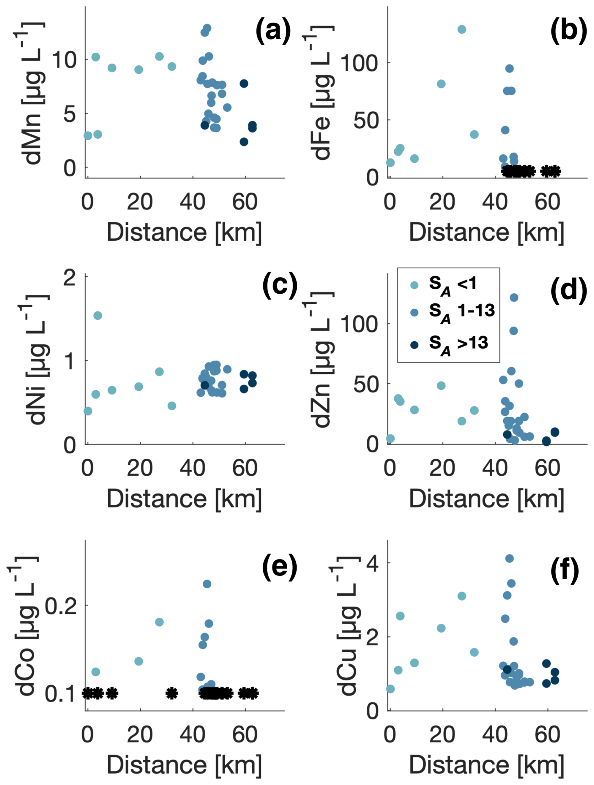
Figure 4 Concentration of dissolved trace metals versus distance from the glacier. Concentration below the quantification limit is shown at the detection limit for each element (*). Data points with salinities in the intervals <1, 1–13, and >13 g kg⁻¹ are shown with colours.

Distributions of dissolved iron (dFe) and dissolved cobalt (dCo) exhibited a similar pattern. However, their distributions were significantly different from the other elements. In general, the dFe concentration increased along the river from 10 to 120 µg L⁻¹ and from 0.12 to 0.19 µg L⁻¹ for dCo. In the highly saline part of the transect, the concentrations ranged from 5 (i.e. the detection limit for dFe) to 100 µg L⁻¹ for dFe and from 0.1 (detection limit for dCo) to 0.24 µg L⁻¹ for dCo. Most of the dFe samples below the detection limits were found in the outer part of the transect (S_A>13 g kg⁻¹).

Dissolved nickel (dNi) showed a distinct pattern, different from the other elements, where concentrations increased slightly from the glacier to the river from 0.5 to 1 µg L⁻¹ (and up to 1.5 µg L⁻¹ for one data point). In the fjord, concentrations appeared constant with all values around 1 µg L⁻¹.

3.2.2 Trace metals versus surface S_A

Salinity in the inner part of the fjord reflected the location of the river plume, and distributions of the tracers versus S_A therefore account for temporal variation of the river plume during the field campaign. Therefore, the distributions were also analysed versus surface S_A (Fig. 5). The distribution of trace metals against salinity exhibited significant differences between the elements. The concentrations for dMn, dCo, and dNi were relatively constant compared to dFe, dZn, and dCu. For dFe, the concentrations were highest at the glacier and in the river (i.e. S_A=0) as well as at two stations (sts. 15 and 16) in the inner part of the fjord (Table A2). Low concentrations were observed in the high-saline part of the transect. Similar patterns were observed for dZn, dCo, and dCu. Manganese showed a relatively gradual decrease from the river and into the fjord; dNi showed minor changes in the fjord.

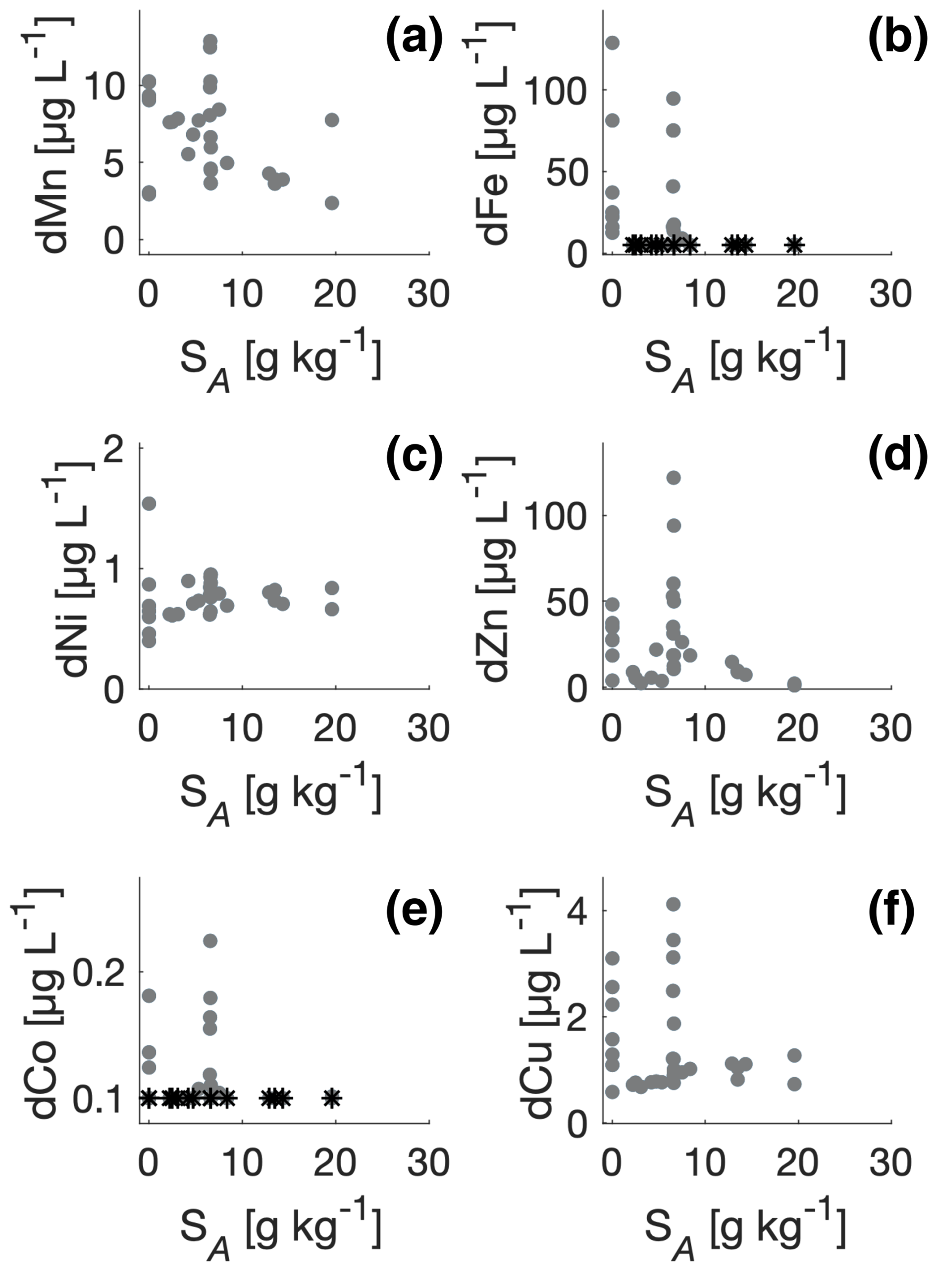
Figure 5 Trace metal concentrations versus surface salinity (S_A). Dissolved manganese (dMn), dissolved iron (dFe), dissolved nickel (dNi), dissolved zinc (dZn), dissolved cobalt (dCo), and dissolved copper (dCu) are shown consecutively in panels (a)–(f). Measurements below detection limits are shown (*).

3.2.3 Trace metals versus freshwater content

Similarly to surface salinity, the freshwater content reflects the position of the river. However, as F_w is determined from the integrated salinity in the surface layer, it is a suitable and less variable representative of the average position of the river plume in the fjord. Trace metal distributions in the fjord were therefore also analysed in relation to the freshwater content. Analysis in relation to F_w was only relevant in the fjord; therefore, the river measurements were not included in relation to F_w.

The highest concentrations of dMn, dFe, dZn, dCo, and dCu were observed at stations with a freshwater content larger than 2.5 m (Fig. 6). That implies that these tracers had the highest concentrations at stations with the largest impact from runoff. The gradient in F_w is dominated by river runoff. The impact of sea ice melt would approximately be equal along the fjord and of the order of 1 m under the assumption of a typical sea ice thickness of 1 m in the fjord. The precipitation on the surface makes a small contribution as this period was relatively dry (Sect. 2.1). Thus, the freshwater gradient decreasing from 3 to 1 m at the outer stations mainly represents river water. At stations with less F_w, the concentrations of dFe and dCo were below or close to the detection limits. The distribution of dNi was relatively constant in the fjord (∼0.8 µg L⁻¹).

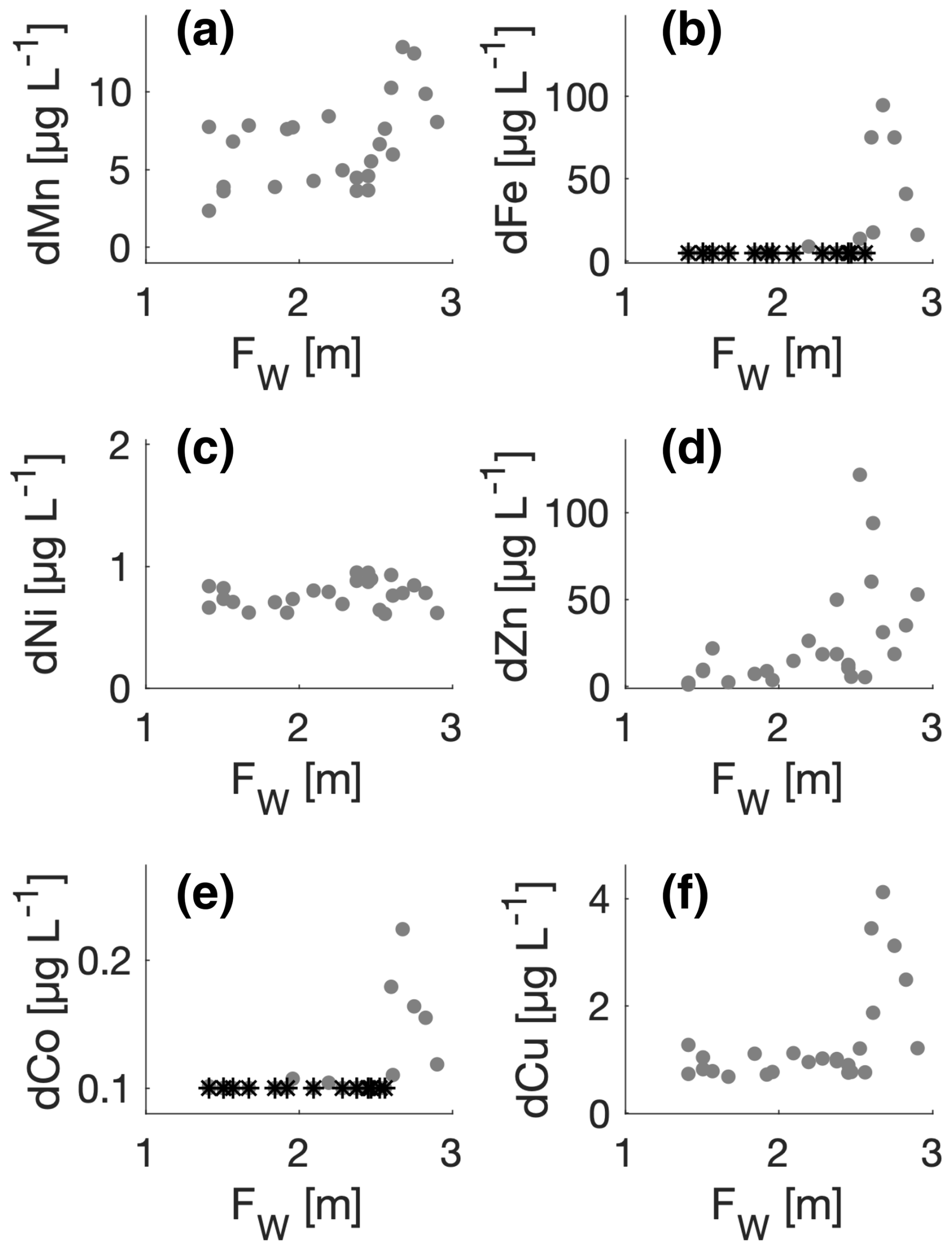
Figure 6 Trace metals versus freshwater content (F_w). Dissolved manganese (dMn), dissolved iron (dFe), dissolved nickel (dNi), dissolved zinc (dZn), dissolved cobalt (dCo), and dissolved copper (dCu) are shown consecutively in panels (a)–(f). Measurements below detection limits are shown (*).

Three trace metals (Mo, V, and U) were analysed in relation to both distance from the glacier and F_w (Fig. 7). All three tracers showed concentrations below the detection limit close to the glacier, and dU was below the detection limit in the entire river (i.e. detection limits of 0.1, 0.5, and 0.1 µg L⁻¹ for dMo, dV, and dU, respectively). Similarly, dMo was relatively low in the river, whereas dV showed elevated concentrations midway between the glacier and the outlet. Concentrations of dMo and dU were low or below the detection limits at stations with an F_w larger than 2.5 m, i.e. stations with the largest impact from runoff. Low concentrations of dV below detection limits were observed at stations with an F_w of less than 2.5 m (i.e. less impacted by runoff); however, some variability characterized its distribution along the transect in the fjord.

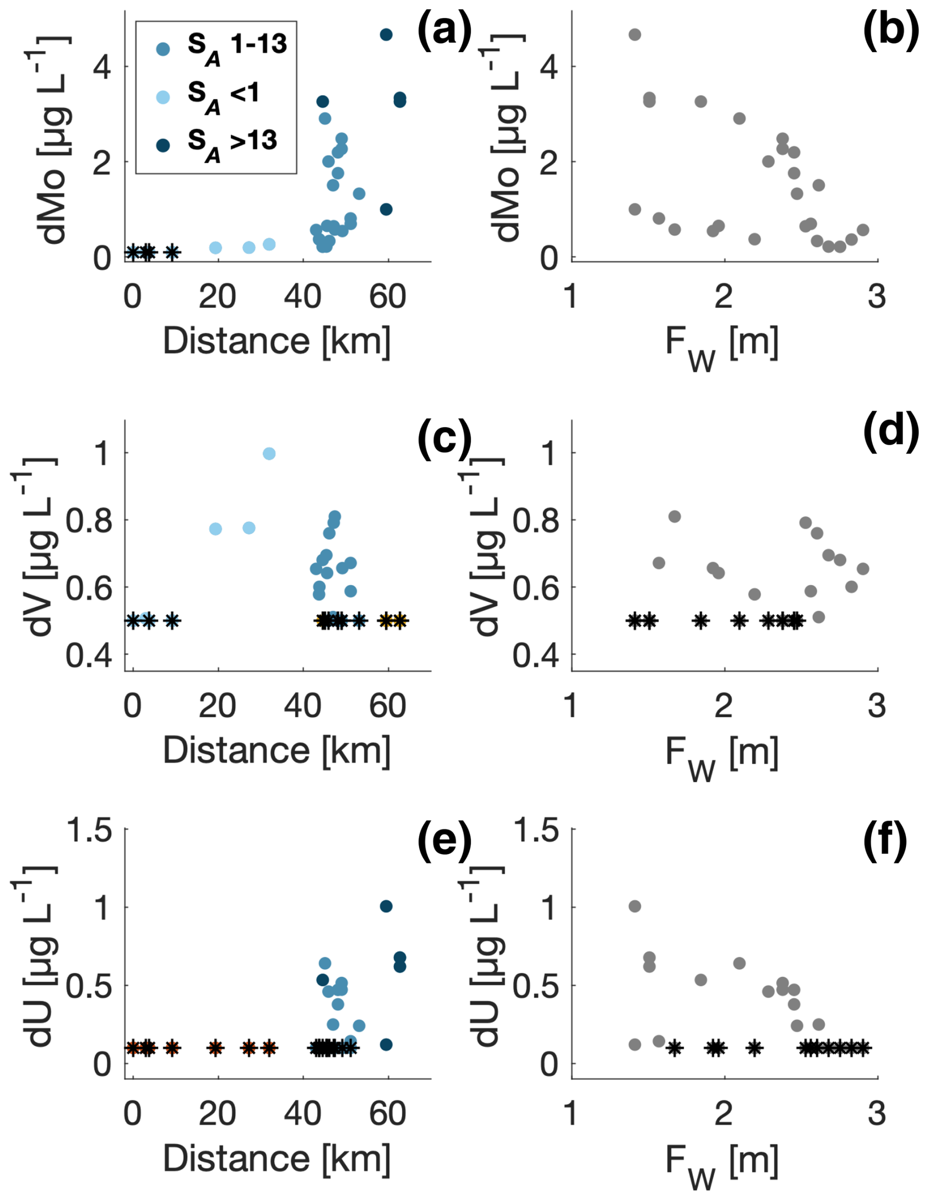
Figure 7 Distribution of dissolved molybdenum (dMo, a), dissolved vanadium (dV, c), and dissolved uranium (dU, e) versus distance from the glacier (km) and freshwater content in the fjord (b, d, f). Data points with salinities in the intervals: <1, 1–13, and >13 g kg⁻¹ are shown with colours in panels (a), (c), and (e). Measurements below detection limits are shown (*).

3.3 Nutrients and SSC distributions

Silicate (Si) was lowest near the glacier, and the largest values were observed in the fjord and ∼40 km from the glacier (Fig. 8). Si concentrations increased gradually from the glacier along the river from 0 to 5 µmol L⁻¹ and obtained the largest value of 10 µmol L⁻¹ at the site before the river delta and closest to the fjord. In the inner fjord, where surface salinity was between 1–13 g kg⁻¹, Si ranged between 5 and 20 µmol L⁻¹ (Fig. 8b). These values were significantly higher than near the glacier and along the river. The Si concentration decreased to 2–7 µmol L⁻¹ at higher salinities. Phosphate and dissolved inorganic nitrogen (DIN, i.e. the sum of ammonia, nitrite, and nitrate), however, showed a more variable relationship with salinity (Fig. 8d and f) with a general decrease towards higher salinities. The vertical nutrient distributions showed that silicate increased near the surface, whereas phosphate and DIN showed very low concentrations in the upper 10 m of the surface layer. Profiles of nutrients showed different distributions with depth (Fig. 9): silicate was highest at the surface and decreased below 10 m. Phosphate and DIN exhibited a similar pattern, where phosphate and DIN concentrations increased with depth and reached high values of ∼0.4 and 5 µmol L⁻¹ at 40 m depth for phosphate and DIN, respectively.

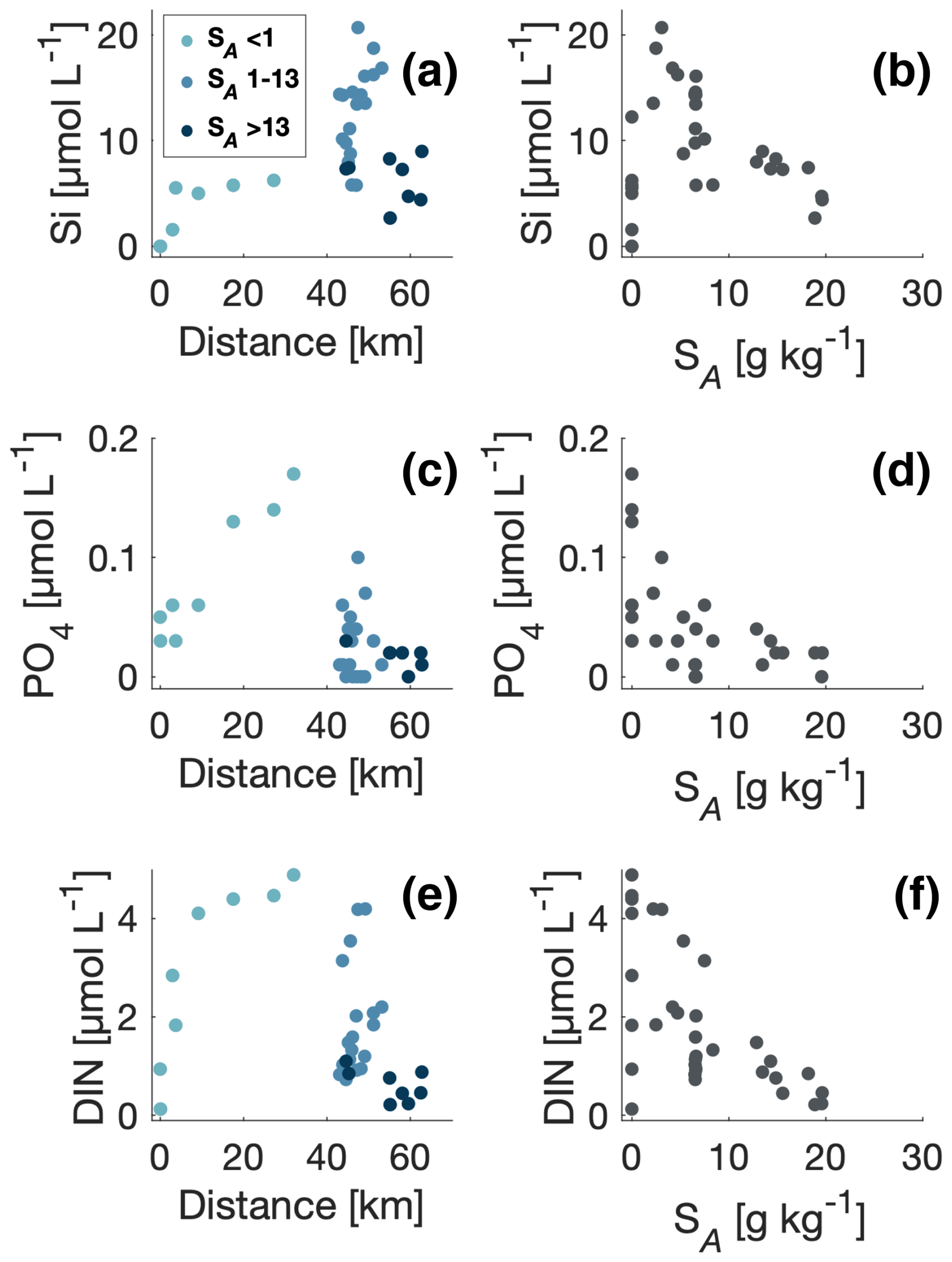
Figure 8 Distributions of (a) silicate, (c) phosphate, and (e) dissolved inorganic nitrogen (DIN) concentrations (µmol L⁻¹) versus distance from the glacier (km). The salinity gradient follows a scale of blue colours, where lower salinity is shown in lighter blue and higher salinity in darker blue. Panels (b), (d), and (f) show the spatial distributions of the same macronutrients based on the salinity gradient.

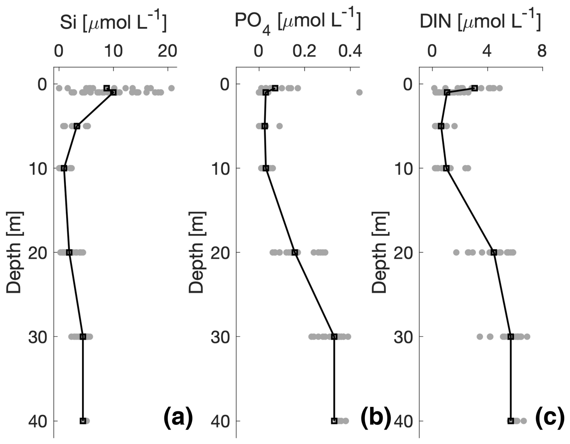
Figure 9 Average distributions of macronutrients (µmol L⁻¹) from all stations in the fjord: (a) silicate, (b) phosphate, and (c) dissolved inorganic nitrogen (DIN). The black lines represent the mean for all stations. The grey points show all the data for all stations at each depth.

The suspended sediment concentration (SSC) was measured at the surface and at 1 m depth (Fig. 10). SSC showed a general decrease from ∼100 mg L⁻¹ in the river and at low salinities to values of ∼10 mg L⁻¹ in the high-saline part of the transect.

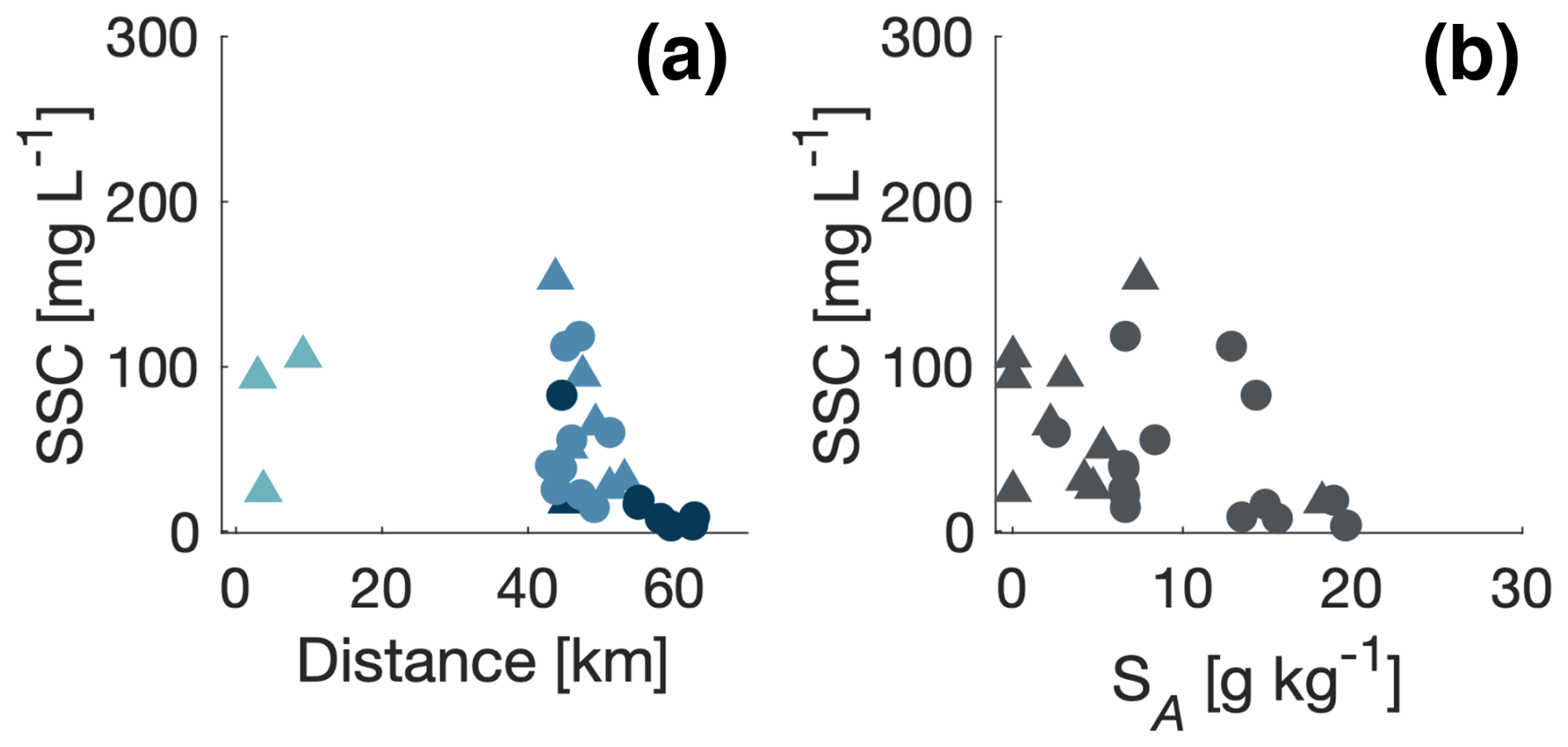
Figure 10 Suspended sediment concentration (SSC) versus distance from the glacier (a) and the surface salinity (b). Data points with salinities in the intervals <1, 1–13, and >13 g kg⁻¹ are shown with colours, where lower salinity is shown in lighter blue and higher salinity in darker blue. Samples taken at the surface (triangles) and at 1 m depth (circles) are indicated. Note that no SSC samples were taken between 10 and 40 km from the ice margin.

4 Discussion

The spatial distribution of trace metals from the glacier to the fjord reflects the complex interactions and impacts from runoff, physical mixing, weathering, erosion, and water–sediment fluxes; the concentration of metal-binding organic compounds, scavenging associated with flocculation, and biological uptake; and remineralization of metal-containing organic matter. Thus, the flux of trace metals in the meltwater river that finally enters the fjord and coastal ocean is heavily influenced by many different processes in the transition zone.

4.1 Trace metal gradients from glacier to fjord

The concentration of dFe showed relatively high values close to the glacier (13 µg L⁻¹) and a tendency to increase along the river (Fig. 4b). The highest value of dFe (129 µg L⁻¹) was observed midway between the glacier and the river delta, suggesting the presence of significant dFe sources along the river (Table A2). One possible explanation is enhanced weathering and metal mobilization or external sources associated with mixing of meltwater from different sub-catchments, e.g. contributions from joining rivers and streams between the glacier and the fjord such as the Leverett Glacier and Ørkendalen river.

This is consistent with recent findings from Hawkings et al. (2020), who reported high concentrations of dFe (up to 20 900 nM, 1170 µg L⁻¹) and large annual fluxes (1.4 Gmol yr⁻¹) from the Leverett Glacier subglacial system. Their study highlights the geochemical reactivity and potential for high trace metal export from this catchment, which drains into the Watson River. Importantly, Leverett Glacier is hydrologically connected to the main meltwater river sampled in this study, strengthening the likelihood that it contributes significantly to the elevated dFe values observed mid-river.

Additional support for Leverett Glacier as a key source comes from Yde et al. (2014), who estimated annual Fe export from the Watson River to be between 15 000 and 52 000 t. Martin et al. (2020) further showed that glacial streams in the region, including those feeding into Watson River, deliver significantly higher DIN and PO₄ than deglaciated streams, with iron concentrations that were comparable and substantial. These findings reinforce the idea that the elevated dFe levels observed here are largely driven by upstream inputs rather than solely by in-stream processes, which are unlikely to explain a near 10-fold increase in concentration along the river.

Similar high dFe concentrations have been observed in other glacial settings in the Greenland Ice Sheet. Bhatia et al. (2013) reported values in the range of 21–56 µg L⁻¹ from glaciers located ∼100 km north of our study site. Zhang et al. (2015) found 6–45 µg L⁻¹ near a glacier in Svalbard. Thus, the high concentration near the glacier and in the river is in general accordance with previous findings that glacier meltwater may carry high concentrations of dFe towards the sea.

Concentrations in the fjord showed a significant decrease of dFe near the river outlet, and it was associated with the location of the river plume. The highest concentrations were observed in areas close to the river where the freshwater content in the upper 15 m was above 2.5 m. Farther from the river outlets and where the freshwater content was below 2.5 m, dFe concentrations were below the detection limit. These patterns are consistent with previous studies which have correspondingly identified the river–seawater transition as an area with a large sink of dFe (Boyle et al., 1977; Zhang et al., 2015). The distribution in the inner fjord showed an elevated concentration off the fjord arm that receives meltwater from the Umivit river. The additional runoff from the Umivit river and the combined mixing from the two river outlets may explain the increased concentration of dFe in the inner part of the fjord where the freshwater content was above 2.5 m (Fig. 6). The distributions also indicated a relatively high dFe concentration in the Umivit river. The low concentration farther out in the fjord was in general accordance with observations in fjords and coastal waters along west Greenland. Hopwood et al. (2016) observed relatively high concentrations (13 µg L⁻¹) in low-salinity water near a glacier and river outlets in Godthåbsfjord (∼65° N) and lower values of ∼2 µg L⁻¹ near the fjord mouth; van Genuchten et al. (2021) observed similarly high dFe values (13 µg L⁻¹) within 10 km of a river outlet in Ameralik fjord (a neighbouring fjord to Godthåbsfjord), while their observations around Disko Island (∼69° N), i.e. an area close to coastal water masses, showed significantly lower values of ∼0.3 µg L⁻¹. However, these values are still significantly larger than typical open ocean concentrations of typically less than 1 nM (=0.056 µg L⁻¹) (Boyd, 2002; Boyd and Ellwood, 2010). Overall, the sharp drop from >100 µg L⁻¹ in river water to <5 µg L⁻¹ in the inner fjord underscores the strong control of mixing and particle scavenging on iron availability in fjord surface waters.

Distributions of dCu and dCo also showed a gradual increase along the river, whereas Mn, Ni, and Zn had initially low concentrations near the glacier and more stable levels downstream. A similar positive relationship with freshwater content was observed for dMn, dZn, dCo, and dCu (Fig. 6). Ni remained relatively constant in the inner fjord at ∼1 µg L⁻¹. Thus, high concentrations in the Umivit river may also explain the increased concentrations of dMn, dZn, dCo, and dCu off the Umivit fjord-arm. Compared to concentrations on the adjacent shelf, fjord values were elevated. Campbell and Yeats (1982) reported surface values (10 m depth) of 4.4, 0.7 and 1.0 µg L⁻¹ for dMn, dNi, and dCu, respectively, on the shelf off Kangerlussuaq fjord (67.75° N, 57.08° W). This study found even higher levels of dMn, dNi, and dCu in the fjord (Table 1). Similarly, dZn concentrations were up to an order of magnitude higher than those observed in Baffin Bay (Colombo et al., 2019). Given the role of Zn in enzymatic degradation of polysaccharides and its influence on dissolved organic matter (DOM) cycling (Helbert, 2017), its elevated levels are particularly noteworthy. Altogether, these observations suggest that the fjord acts as a source of trace metals for coastal surface waters.

In contrast, dMo, dV, and dU showed low concentrations near the glacier. All dU values in the river were below the detection limit, with the highest concentrations occurring at the high-salinity outer-fjord stations. There was no, or below detection limit levels of, dU in the surface water near the innermost stations with freshwater content above 2.6 m (Fig. 7e and f). This indicated that the primary source of dU is likely coastal water intrusion or exchange with fjord bottom waters. The distribution of dV varied both in the river and in the fjord; however, the outermost stations showed values below the detection limit, and this was also the case for dMo, further suggesting limited riverine input.

4.2 Nutrients and biological production

The river distributions of macronutrients silicate, phosphate, and DIN all showed a general increase along the river, indicating additional inputs between the glacier and the fjord, likely from lake runoff or organic matter remineralization. The concentrations of DIN and phosphate in the river were higher than the surface concentrations in the fjord, which showed that the transport of these macronutrients in the river is important for the cycling and biological uptake in the inner part of the fjord. The vertical distribution of DIN and phosphate showed relatively low values in the upper 10 m, likely due to biological uptake following sea ice breakup. Silicate concentrations, in contrast, were significantly higher in the fjord than in the river, pointing to internal sources, such as the weathering of glacially derived fine material (GRF), as proposed by Hawkings et al. (2017), or from biological cycling. A silicate minimum between the surface and 30 m supports the idea of uptake by diatoms. These observations suggest that silicate weathering may play an important role in shaping nutrient and trace metal dynamics in this region, underscoring the need for further investigation into its contribution. Trace metals also influence productivity by serving as cofactors in enzymatic and photosynthetic processes. For example, manganese and nickel are vital for metabolic pathways, including carbon fixation and nitrogen cycling. Elevated levels of these metals in the inner fjord, particularly during peak meltwater discharge, could enhance microbial and phytoplankton productivity, linking meltwater-driven geochemistry to ecosystem responses.

4.3 Future perspectives

Understanding sinks in this saline region of the fjord is crucial, as a significant portion of the dissolved inorganic compounds are removed from the water column. This study offers insights into the pathways and processes that regulate trace metal and nutrient dynamics in the transition zone in glacier-influenced fjord systems. Furthermore, the variability in meltwater discharge and sediment plumes over time highlights the importance of continuous monitoring to capture seasonal and interannual trends.

Further research incorporating the biological response to trace metal inputs from glacial discharge would help clarify the broader ecosystem impacts, particularly as glacial melt accelerates. Estimating the concentrations of trace metals entering the ocean from glacial discharge remains challenging, and this study, uniquely covering the transition from glacier to fjord in Greenland, underlines the importance of the transition zone and the associated sinks that must be considered when modelling or extrapolating riverine transport into the oceans.

Appendix A

Table A1 Water sampling locations from the GROFS1 field campaign. Trace metals were collected at stations 6–35 (excluding sts. 12 and 29). Time is shown as western Greenland time (WGT). Depths are from the echo-sounder-resolved depths down to ∼200 m, and at some deeper stations the depth was not resolved. Distances are measured from the glacier. Area type is defined in Table 1. Surface salinity (S_A) was bin-averaged between 0.5–1.0 m depth, and the freshwater content (F_w) was calculated in the upper 15 m.

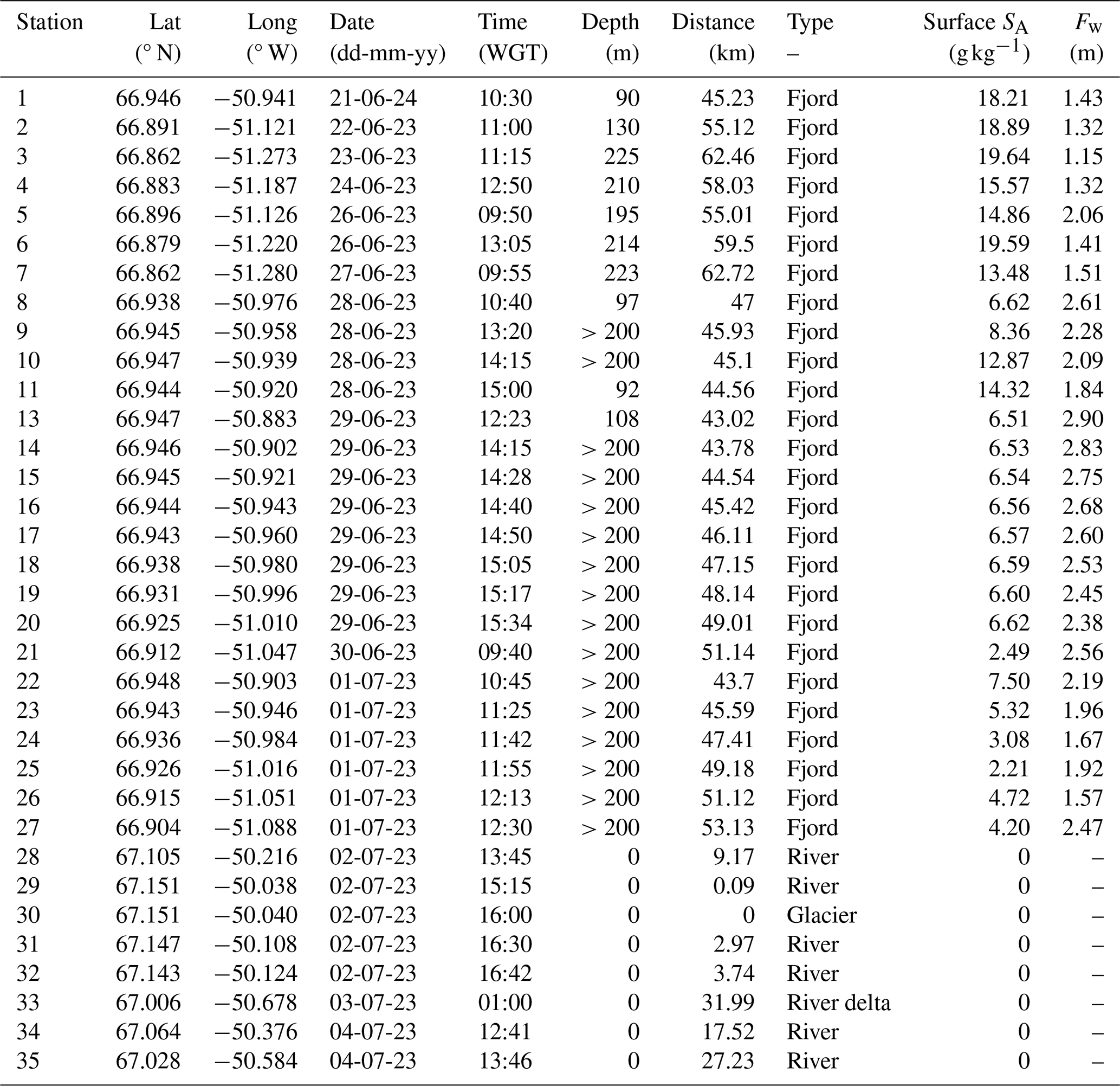
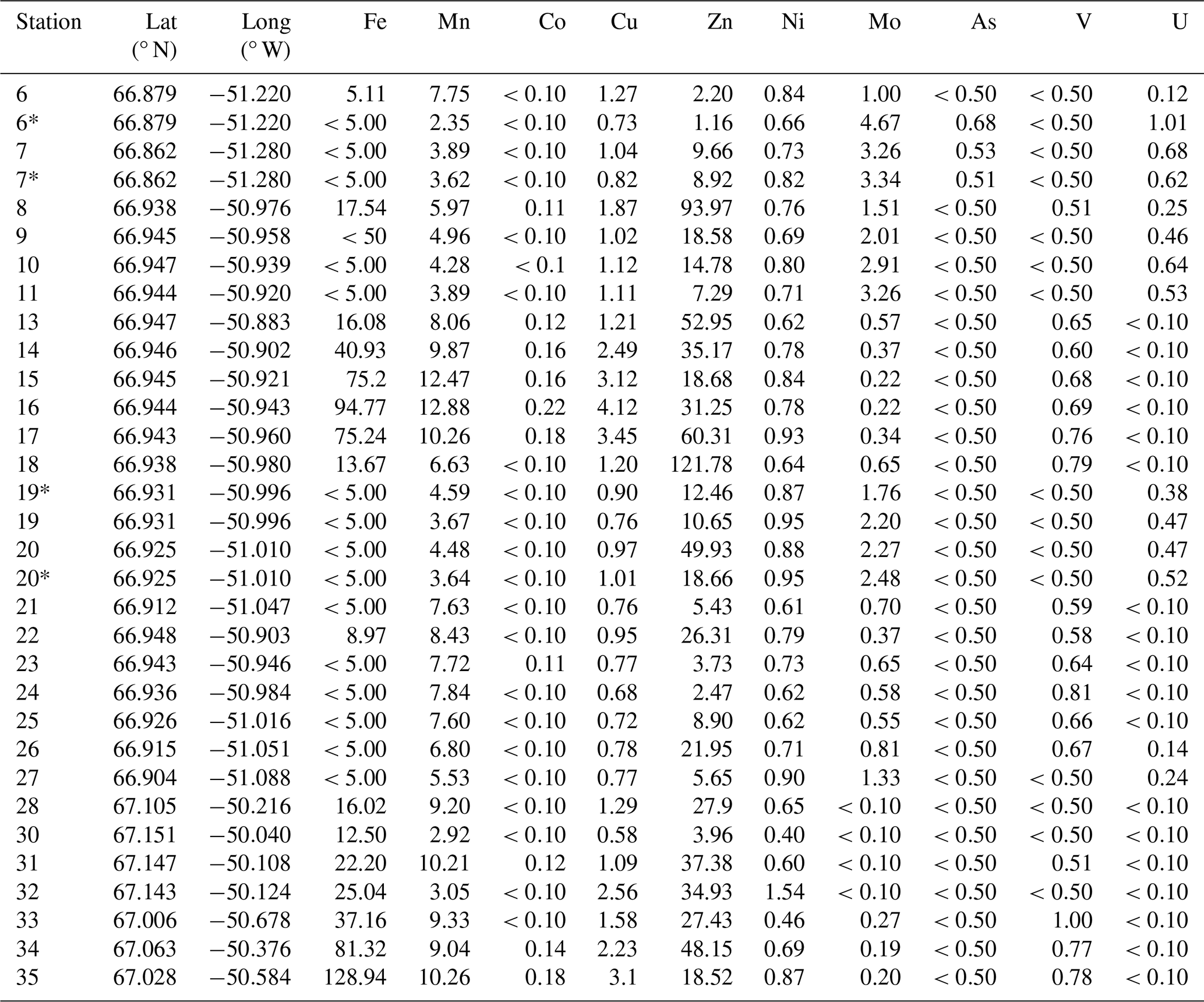
Table A2 Trace metal data (µg L⁻¹); iron (Fe), manganese (Mn), cobalt (Co), copper (Cu), zinc (Zn), nickel (Ni), molybdenum (Mo), arsenic (As), vanadium (V), and uranium (U). Values below quantification limit are shown as “< quantification limit value” for each element, respectively. Chromium (Cr) and lead (Pb) presented mostly all values below quantification limit except for stations 17 and 35, where Cr was 0.52 and 3.25 µg L⁻¹, respectively. Pb was 0.10 µg L⁻¹ at station 17. (*) Two samples were taken at stations 6, 7, 19, and 20. Instrument uncertainties are shown in Table S1.