Estimation of duration and its changes in Lagrangian observations relying on ice floes in the Arctic Ocean utilizing a sea ice motion product

Since the 1890s, buoy- and camp-based Lagrangian observations relying on ice floes have been indispensable for data acquisition in the difficult-to-access central Arctic Ocean in winter. Evaluating the potential observation duration, and how it changes in association with changes in the Arctic climate system, is crucial for planning ice camp or buoy deployment. Using a remote sensing sea ice motion product, we reconstructed sea ice drift trajectories for each annual cycle from 1979–1980 to 2022–2023 and identified ideal areas for ice camp or buoy deployment in the central Arctic Ocean. The results show that, based on the setup time of 1 October, areas centered at 82° N and 160° E, near north of the East Siberian and Laptev seas, with a size of 7.0 × 10⁵ km², could ensure Lagrangian observations for at least 9 months, with the drifting remaining in the ice zone and not entering the exclusive economic zones (EEZs) of Arctic coastal countries, with the probability of 75.0 %–90.9 % over 44 years. The potential deployment areas favored ice advection to the Transpolar Drift (TPD) region relative to the Beaufort Gyre (BG) region. Ice trajectory terminal points did not reveal an obvious long-term tendency, but they were regulated by large-scale atmospheric circulation patterns, especially those in the early drifting stage in autumn (OND). In particular, the autumn east–west surface air pressure gradient across the central Arctic and the Arctic dipole anomaly indices significantly influenced the terminal points of ice trajectories after 9 months, and their extreme positive phases were found to expand the ideal deployment areas. The rate of increase in near-surface air temperatures in autumn–spring along the trajectories was more pronounced in the TPD region than that in the BG region. The sea ice response to wind stress significantly intensified in recent Lagrangian observations, suggesting stronger ice dynamic processes as the sea ice thins. The geopolitical boundaries of EEZs have a significant impact on the sustainability of the Lagrangian observations, limiting them to a maximum of 10 months. Without this restriction, the potential Lagrangian observations in the BG and TPD regions would expand southward, with an increased duration by 20.5 and 5.0 d, respectively, compared to those with the EEZ restriction.

1 Introduction

Arctic sea ice, a crucial indicator and amplifier for climate change (Kwok, 2018), has experienced pronounced change, becoming progressively thinner and younger, with its extent in September declining by 13 % per decade during the satellite observation era since 1979 (Parkinson and DiGirolamo, 2021; Meier and Stroeve, 2022; Babb et al., 2023). State-of-the-art Earth system models show significant spread in projecting the evolution of Arctic sea ice (Holland and Hunke, 2022), mainly due to insufficient observational data for the parameterization of sea ice thermodynamic and dynamic processes (Smith et al., 2022), a severe absence of reliable observational data for assimilation (Liu et al., 2019), and the rough treatment of Arctic snow and sea ice processes in atmospheric reanalysis data (Batrak and Müller, 2019). The frozen ocean and extremely harsh weather limit the accessibility of the central Arctic Ocean, exacerbating the data scarcity of ship-based oceanography measurements. This situation is even worse in the freezing season (Rabe et al., 2022).

Lagrangian measurements from ice camps or buoys deployed on ice floes provide an alternative means of observing the interactions between the atmosphere, ice, and ocean in the Arctic. In the 1890s, Fridtjof Nansen and his companions pioneered Lagrangian observations in the central Arctic Ocean using the ice camp and wooden galleon, which provided the first basic depiction of Arctic sea ice and oceanic physical regimes. Subsequent ice-camp-based campaigns include the Ice Station Alpha (Cabaniss et al., 1965), the Arctic Ice Dynamics Joint Experiment (AIDJEX; Coon, 1980), the Surface Heat Budget of the Arctic Ocean (SHEBA) campaign (Uttal et al., 2002), as well as the Norwegian young sea ICE (N-ICE2015) Expedition (Granskog et al., 2016). These efforts provided vital observational data for constructing theoretical frameworks of sea ice physics as well as parameterizing sea ice thermodynamic and dynamic processes and heat and/or salt exchanges with the lower atmosphere and/or upper ocean, enabling the development of sea ice numerical models. The Soviet Union–Russia Arctic ice-camp project, lasting for several decades since the 1930s, has provided the climatological characteristics of extensive snow and sea ice geophysical variables over the central Arctic Ocean (Frolov et al., 2005), supporting numerical simulations (e.g., Tian et al., 2024) and remote sensing retrieval algorithms of Arctic sea ice (e.g., Lavergne et al., 2010). Recently, the Multidisciplinary drifting Observatory for the Study of the Arctic Climate (MOSAiC) fully leverages the advantages of multidisciplinary observations on ice floes, which serve as an intermediate medium (Nicolaus et al., 2022; Rabe et al., 2022; Shupe et al., 2022), marking a milestone for Arctic drifting observation campaigns.

However, the implementation of an ice camp, accompanied by a modern icebreaker such as the MOSAiC, requires a significant logistical budget; without the icebreaker support, like in the Soviet Union-Russia ice camps, camps face significant risks including from ice floe fragmentation, storms, and polar bears. These factors all limit the sustainable implementation of ice camps. It is gratifying that Arctic ice floes provide a broad platform without the need for extra floatation support for deploying buoys or other observation instruments. Various types of buoys have been designed and deployed in the Arctic Ocean to measure sea ice kinematics (Lukovich et al., 2011), snow and sea ice mass balance processes (Richter-Menge et al., 2006; Jackson et al., 2013; Nicolaus et al., 2021; Lei et al., 2022), meteorological parameters and heat exchanges over the ice surface (Cox et al., 2023), as well as oceanic temperature, salinity profiles, and turbulence heat flux underneath the ice (Shaw et al., 2008; Toole et al., 2011). The co-deployment of various types of buoys on the same floe to obtain a comprehensive observation matrix comprising multiple media (e.g., Morison et al., 2002), or at a local scale of tens of kilometers (e.g., Rabe et al., 2024), can help match the grid scales of satellite remote sensing (e.g., Koo et al., 2021) and numerical models (e.g., Pithan et al., 2023). Such a task is extremely hard to achieve in open water.

The effective duration of Lagrangian observations relying on ice floes, and the observation regions they may drift through, is highly dependent on the setup or deployment location of the ice camp or buoy. This is because Arctic sea ice advection is primarily regulated by two surface ocean circulation systems – the Beaufort Gyre (BG) and Transpolar Drift (TPD) (Kwok et al., 2013). Remote sensing sea ice motion (SIM) products can be used to simulate forward (backward) ice drift trajectories to track the destinations (origins) of ice floes (Lei et al., 2019) or estimate ice age by tracking the duration of ice drifting (Tschudi et al., 2020). Krumpen et al. (2019) analyzed interannual variations in advection patterns based on reconstructed ice trajectories using a Lagrangian tracking approach. They further investigated the impacts of ice advection patterns on ice mass or ice-associated material transmission in the TPD region. Based on this, Krumpen et al. (2020) estimated the origin of the ice floe used to setup the MOSAiC ice camp, in order to support interdisciplinary observations at the ice camp. In the practical process of establishing the MOSAiC ice camp, the reconstructed ice drift trajectory using the SIM product served as an important basis for selecting the deployment location. From the perspective of logistics, Granskog et al. (2016), Nicolaus et al. (2022), and Rabe et al. (2024) emphasize how the dynamic deformation of ice floes can affect the safety of observation equipment deployed at ice camps. However, there is a lack of a comprehensive assessment of how deployment locations influence the subsequent drifting and destinations of ice camps and buoys at the basin scale in the Arctic Ocean. This study aims to address this gap by identifying the ideal deployment regions for ice camps or buoys using a SIM product. The goal is to ensure uninterrupted observations while avoiding risks such as drifting to the ice edge or into the exclusive economic zone (EEZ) of a country that is not involved in the observation experiment before the end of the expected duration.

During the Lagrangian observations, atmospheric thermodynamic and dynamic forcing not only determine the seasonal evolution of the sea ice itself, but they also affect the heat and momentum exchanges between the atmosphere and sea ice. They can provide important context for interdisciplinary studies based on Lagrangian observational data (e.g., Krumpen et al., 2021; Rinke et al., 2021). Given Arctic amplification and the sustained loss of Arctic sea ice, understanding climatological characteristics and long-term trends in atmospheric forcing and sea ice kinematics along the potential drifting trajectory is essential for planning the deployment of ice camps or buoys. Moreover, there is widespread consensus that some atmospheric circulation patterns play a critical role in regulating Arctic sea ice advection. The Arctic Oscillation (AO) (Thompson and Wallace, 1998) regulates the axis alignment of the TPD and the extent of BG. During positive (negative) AO phases, the axis alignment of the TPD tends to shift westward (eastward), and the BG shrinks (expands) (Rigor et al., 2002). The wind anomalies induced by the dipole anomaly (DA) (Wu et al., 2006) exhibit strong meridional forcing in the TPD region, with positive (negative) phases accelerating (decelerating) the sea ice drift along TPD (Wang et al., 2009). The Central Arctic air pressure gradient Index (CAI), defined as the east–west gradient of sea-level air pressure (SLP) across the central Arctic Ocean, could regulate partly regulate meridional wind forcing parallel to TPD (Vihma et al., 2012). The Beaufort High (BH) (Moore et al., 2018) is closely associated with sea ice circulation in the BG region (Proshutinsky and Johnson, 1997). These atmospheric circulation patterns affect the sea ice drift trajectory and advection direction through various mechanisms and, consequently, affect the duration of Lagrangian observations relying on ice floes. Thus, their regulatory mechanisms and seasonal variations need further clarification when evaluating the duration of Lagrangian observations using Arctic ice floes.

In this study, we organized the sections as follows. The datasets and methods used to reconstruct sea ice drift trajectories and estimate changes in atmospheric and ice conditions along the trajectories are briefly described in Sect. 2. The ideal deployment areas for Lagrangian observations, as well as the changes in atmospheric thermodynamic and dynamic forcing along the potential ice trajectories during each annual cycle from 1979–1980 to 2022–2023 (hereinafter referred to as 1979–2022), are presented in Sect. 3. The performance of the reconstruction method, the relation between the ice trajectories and atmospheric circulation patterns, and the impact of EEZ constraints and deployment time on the sustainability of Lagrangian observations are discussed in Sect. 4. Conclusions are given in the last section. This study provides an important cognitive foundation for the planning and implementation of Lagrangian observations relying on ice floes in the central Arctic Ocean.

2 Data and methods

2.1 Study area

Our study focuses on the reconstruction of sea ice drift trajectories in the central Arctic Ocean, because it is difficult to maintain sufficient drifting observation time in the peripheral sea. Here, the central Arctic Ocean is defined as the high Arctic that is excluded from the EEZs of any country, determined using the maritime boundary polylines (version 12) of the geodatabase provided by the Flanders Marine Institute. To define potential areas for preferred deployment sites, we identified a rectangular area of 1.44 × 10⁶ km², consisting of 2294 pixels on the 25 km polar stereographic grid, with area corners aligned with the EEZ boundary polylines, and which covers approximately 53.5 % of the central Arctic Ocean defined in this study (Fig. 1). The definition of such a rectangular area can effectively reduce computational costs related to surveying the entire central Arctic Ocean. To demonstrate its rationality, we surveyed the entire central Arctic Ocean for potential preferred areas for ice camp or buoy deployment using the 1979–2023 climatology of the SIM field. The results revealed that the defined rectangular area contained 91.6 % of the effective starting points for the deployment of an ice camp or buoy with a drifting trajectory of ≥9 months, while avoiding drifting into EEZs or beyond the ice zone, which is higher than that (36.0 %) for other regions within the central Arctic Ocean. Even during the most recent decade of 2013–2023, a period facing more severe and complex challenges due to thinner and younger ice, the rectangular area still contained 25.6 % of effective starting points, while other regions had none. Thus, in other regions within the central Arctic Ocean beyond our defined rectangular area, it is extremely difficult to identify suitable areas to deploy ice camps or buoys to maintain sufficiently long Lagrangian observations. To save computational costs, we believe that defining this rectangular area for the reconstruction and analysis of sea ice drift trajectories in specific years is representative and reasonable. Based on the 1979–2023 climatology of the Arctic SIM field, we roughly defined boundaries to separate the BG and TPD regions, as shown in Fig. 1.

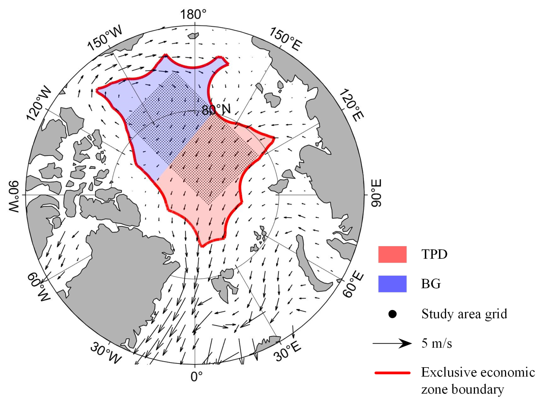
Figure 1 Study area. The black dots indicate grid points that identify the optimal area for buoy or camp deployment. The arrows depict the mean SIM vectors from 1979 to 2023. The region delineated by the red lines represents the central Arctic Ocean, which is defined as the high Arctic excluding the EEZs. The shaded blue and red areas roughly denote the Beaufort Gyre and Transport Drift regions within the central Arctic Ocean.

2.2 Data

2.2.1 Sea ice data

Due to the difficulty of obtaining long-term, large-coverage SIM fields from high-resolution remote sensing images (e.g., Li et al., 2022; Fang et al., 2023), we used the 25 km Polar Pathfinder version 4.1 Sea Ice Motion Vectors from the U.S. National Snow and Ice Data Center (NSIDC; Tschudi et al., 2020), which are suitable for large-scale trend analysis to reconstruct sea ice drift trajectories originating from the study area in 1979–2022. The Global Sea Ice Concentration Climate Data Records from the European Organization for the Exploitation of Meteorological Satellites Ocean and Sea Ice Satellite Application Facility (EUMETSAT OSI SAF; Lavergne et al., 2019) is utilized to evaluate ice conditions along the trajectory. This sea ice concentration (SIC) data are derived from the Scanning Multichannel Microwave Radiometer (SMMR), Special Sensor Microwave Imager (SSM/I), and Special Sensor Microwave Imager/Sounder (SSMIS) passive microwave satellite series sensors. The SIM and SIC data are projected onto the 25 km polar stereographic grid.

2.2.2 Buoy data

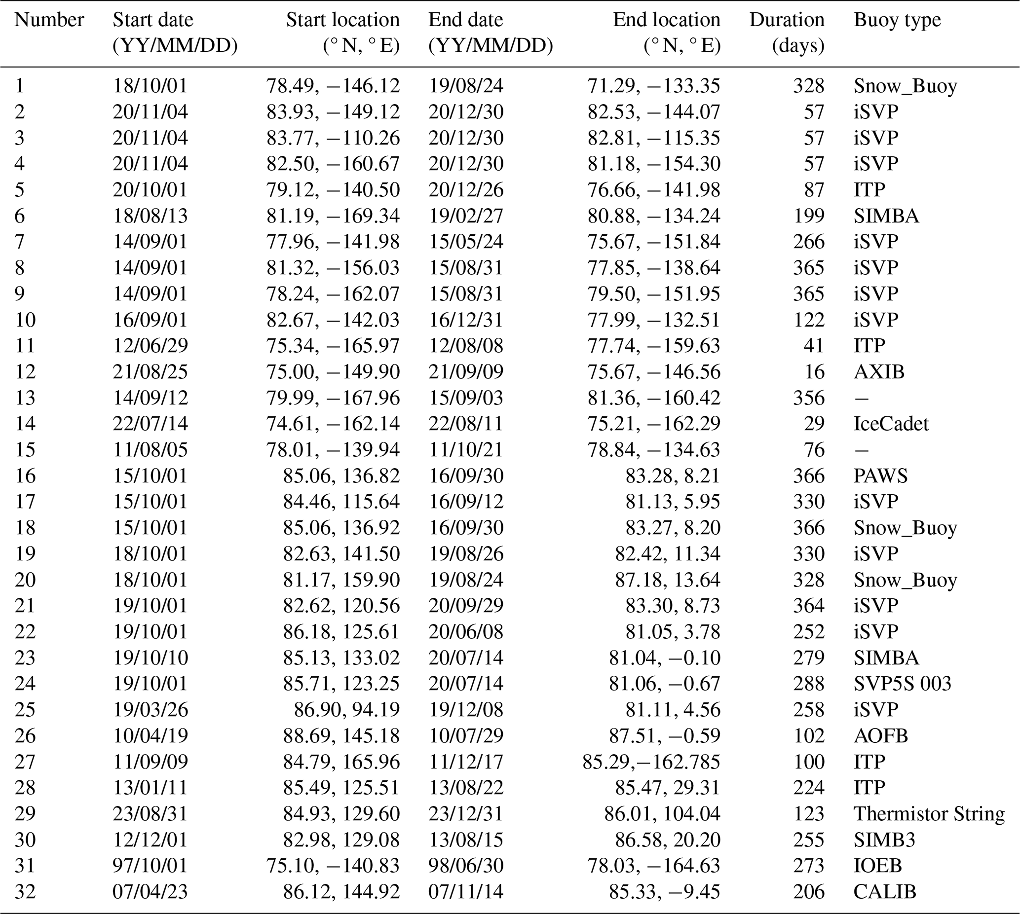
The trajectories of the buoys deployed over the Arctic ice were utilized to validate the reconstructed ice trajectories. To ensure the quality of the validated SIM product, we constrained buoy selection to those situated 100 km offshore within the Arctic Ocean and excluded those south of the Fram Strait. The data of these buoys were derived from the International Arctic Buoy Programme (IABP), the SHEBA, the DAMOCLES (Brümmer et al., 2011), the German Arctic Research Expedition, and the Chinese National Arctic Research Expedition (CHINARE) during the summers of 2014, 2016, and 2018. The data collected by 32 buoys from 1997 to 2023, with 16 in the BG and TPD regions each, were utilized for validating reconstructed ice trajectories in this study. The details are given in Table A1.

2.2.3 Atmospheric data

Atmospheric conditions were examined using atmospheric reanalysis data from the European Centre for Medium-Range Weather Forecasts Reanalysis v5 (ERA5; Hersbach et al., 2020). Hourly near-surface (2 m) air temperature, 10 m wind, snowfall, total precipitation, and surface longwave radiation at about 30 km horizontal resolution were bilinearly interpolated to derive daily atmospheric conditions along the trajectories. ERA5 data is the next generation of the ERA-interim product. It has significantly improved temperature and wind fields for the Arctic Ocean (Graham et al., 2019b), and is able to reasonably characterize snowfall and precipitation (Wang et al., 2019) as well as the surface net longwave radiative flux under various weather conditions (Graham et al., 2019a).

The seasonal (autumn (OND: October, November, and December), winter (JFM: January, February, and March), and spring (AMJ: April, May, and June)) indices of AO, DA, CAI, and BH were used to characterize how atmospheric circulation patterns regulate ice trajectories. The AO and DA indices were calculated from the first and second empirical orthogonal functions of the SLP anomalies north of 70° N, utilizing monthly SLP from the National Centers for Environmental Prediction/National Center for Atmospheric Research to maintain consistency with previous studies (Wu et al., 2006; Wang et al., 2009). Hourly SLP from the ERA5 reanalysis was used to calculate the monthly CAI (Vihma et al., 2012), defined as the difference between SLP at 90° W, 84° N, and 90° E, 84° N. According to Moore et al. (2018), the ERA5 SLP anomaly over the region of 75–85° N and 170° E–150° W were utilized to define the BH index, which is more compatible with the BG from the perspective of sea ice circulation.

2.3 Methods

To assess the effective Lagrangian observation time, determining a survival time (ST) threshold for floes drifting within the Arctic ice region and avoiding entering EEZs is crucial. Based on a given ST threshold, regular grids (Fig. 1) were established as the starting point for ice trajectory reconstruction to identify preferred potential deployment areas of buoys or ice camps. Reconstructed ice trajectories from these areas start on 1 October, aligning with the approximate onset of the ice surface freezing season (Markus et al., 2009) and the setup time (3 October) of the MOSAiC ice camp (Nicolaus et al., 2022). According to Lei et al. (2019), the ice drift trajectories were reconstructed as follows:

$$\begin{array}{}\text{(1)}& {\displaystyle }X\left(t\right)=X\left(t-\mathrm{1}\right)+U(t-\mathrm{1})\cdot {\mathit{\delta }}_t,\text{(2)}& {\displaystyle }\mathrm{and}Y\left(t\right)=Y\left(t-\mathrm{1}\right)+V(t-\mathrm{1})\cdot {\mathit{\delta }}_t,\end{array}$$

where X and Y are the zonal and meridional coordinates of ice trajectories, U(t) and V(t) are the ice motion components at time t along the ice trajectories, and δ_t is the calculation time step of one day. The sea ice drift velocity field is dynamically interpolated at each integration step using bilinear interpolation, which preserves instantaneous spatial variations but may smooth out small-scale features due to a grid resolution of 25 km. For the NSIDC SIM product used in this study, although there are errors in the individual motion estimates, these errors do not accumulate over long-term tracking because the motion estimates are largely unbiased (Tschudi et al., 2020). This is supported by Tschudi et al. (2010), who found a 27 km drift error over 293 d of tracking when compared to SHEBA buoy trajectories, suggesting that errors can still be maintained within limits over long-term tracking. The validation of the reconstructed trajectories with buoy trajectories is provided in Sect. 4.1.

When ice floes enter a region with a SIC < 15 % or the EEZ of a country, the reconstructed ice trajectory is terminated. The time from 1 October to the terminal point is defined as the ST of the ice floe, representing the effective working duration of an ice camp or a buoy that is deployed on it. Note that this study truncated reconstructed ice trajectories exceeding one year (after 30 September of the following year) to focus on identifying areas unsuitable for deploying an ice camp or buoy where the ST of the reconstructed trajectory did not meet the threshold.

As the SIM products were projected onto a 25 km polar stereographic grid, and a rectangular area based on this grid was used as the starting point for ice trajectory reconstruction, the proportion of effective starting points relative to the total grid points, which meet a given ST threshold, can be considered equivalent to the area ratio for the study region. As shown in Fig. 2a, for a 10-month ST threshold, the available deployment areas in the central Arctic Ocean that have a ST not less than 10 months, and a probability >75 % during 44 study years, are very limited (21.6 % of the rectangular study region). This is less than the 48.6 % area when the ST threshold is set as 9 months. The probability of a relatively short duration (less than 180 d) was 1.9 % for the effective region corresponding to a 6 month ST threshold. This was reduced to a negligible value of 0.8 % (1.1 %) for the 10-month (9-month, not shown) ST threshold. However, the probability of a relatively long duration (365 d or beyond) was 70.9 % for the ST threshold of 6 months, which increased to 82.6 % (77.8 %) for the 10-month (9-month, not shown) ST threshold (Fig. 2b). Therefore, to ensure a broad range of deployment areas, i.e., with a probability of >50 % across the entire study region, and ensure sufficient duration for Lagrangian observations, we used a 9-month ST threshold for the subsequent analyses. This means that the ST lasts until the end of June in the year following the deployment, which is close the first drifting phase of the MOSAiC ice camp (Nicolaus et al., 2022). With this ST threshold, almost all the peripheral areas of our defined rectangular region are identified as unsuitable for ice camp and buoy deployment (Fig. 2a). This again proves that it is difficult to identify suitable sites for ice camp or buoy deployment in regions beyond our defined rectangular region in the central Arctic Ocean. It also confirms the rationality of our definition of this rectangular region.

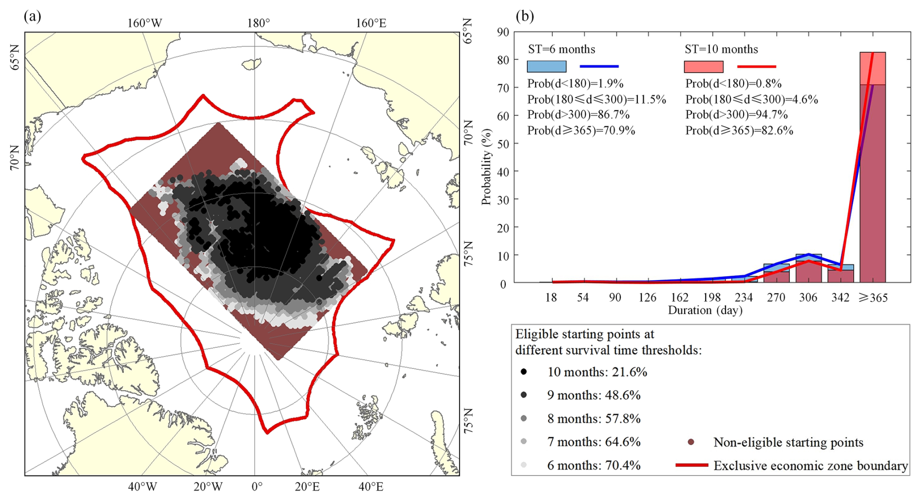
Figure 2 (a) Spatial distribution of eligible starting points and (b) probability distribution of duration according to different thresholds of survival time in 1979–2022. Note that the reconstructed ice trajectories in this study are truncated at one year, until 30 September next year. Thus, for the proportion with a duration ≥365 d, the ice trajectory was still valid by 30 September of the following year.

To verify the reliability of the reconstructed ice trajectories, Euclidean distance and cosine similarity with the buoy observations are used to quantify their distance and direction deviations. The Euclidean distance (D_f) is defined as follows:

$$\begin{array}{}\text{(3)}& D_f=\sqrt{(x_{\mathrm{buoy}}-x_{\mathrm{cal}}{)}^{\mathrm{2}}+(y_{\mathrm{buoy}}-y_{\mathrm{cal}}{)}^{\mathrm{2}}},\end{array}$$

where the subscripts of buoy and cal denote the coordinates of the buoy trajectory and the reconstructed ice trajectory, respectively. The distance deviation is mainly measured using the Euclidean distance between the two trajectories at the endpoint, the average misalignment distance at the corresponding time, and the root mean square error (RMSE). The Fréchet distance (Devogele et al., 2017) and cosine similarity are used to assess directional deviations in reconstructed trajectories. The Fréchet distance quantifies the trajectory similarity by comparing both spatial location and the sequential placement of points, where smaller values indicate better reconstruction accuracy. Cosine similarity is an effective metric for assessing the geometrical similarity between the reconstructed trajectories and buoy trajectories (Gui et al., 2020), where a value approaching one denotes a high similarity between them. The cosine similarity (S_c) between the coordinate vectors of the reconstructed trajectory (Q_cal) and buoy measurement (Q_buoy) is calculated as follows:

$$\begin{array}{}\text{(4)}& S_{\mathrm{c}}={\displaystyle \frac{{\mathit{Q}}_{\mathrm{cal}}\cdot {\mathit{Q}}_{\mathrm{buoy}}}{\left|\left|{\mathit{Q}}_{\mathrm{cal}}\right|\right|\left|\left|{\mathit{Q}}_{\mathrm{buoy}}\right|\right|}},\end{array}$$

where ${\mathit{Q}}_{\mathrm{cal}}=\left(x_{\mathrm{cal}}\left(i\right)y_{\mathrm{cal}}\right(i\left)\right)(i=\mathrm{1},\mathrm{2},\mathrm{3}\mathrm{\dots })$ and ${\mathit{Q}}_{\mathrm{buoy}}=\left(x_{\mathrm{buoy}}\left(i\right)y_{\mathrm{buoy}}\right(i\left)\right)(i=\mathrm{1},\mathrm{2},\mathrm{3}\mathrm{\dots })$.

To characterize regional differences between the BG and TPD regions, we defined starting points based on the geometric centers of grid points with a high probability (greater than 90 %) of reaching the BG or TPD regions (BG: 80.04° N 157.71° W; TPD: 83.31° N 155.94° E). We also identified an ambiguous region with a probability of 40 %–60 % for reaching both regions (both: 81.10° N, 177.89° E). We reconstructed the ice trajectory originating from these regions over 9 months for each cycle from 1979 to 2022 (Fig. 3). The atmospheric thermodynamic forcing, including freezing degree days (FDDs) and thawing degree days (TDDs), snowfall, and precipitation, which are closely related to ice thermodynamic growth and melting processes (Ricker et al., 2017a; Bigdeli et al., 2020), as well as the surface net longwave radiative flux, which is related to the feedbacks of clouds and the sea ice itself on the near-surface atmosphere (Graham et al., 2017), were estimated along the reconstructed ice trajectories. FDD (TDD) refers to the integral of daily average near-surface air temperatures below 1.8 °C (above 0 °C) over the study period, derived from ERA5 hourly air temperatures. These have a negligible bias (7.18 × 10⁻⁷ K) compared to the daily air temperatures obtained directly from ERA5. The dynamic response of sea ice to atmospheric forcing is characterized using the ice–wind speed ratio (e.g., Herman and Glowacki, 2012).

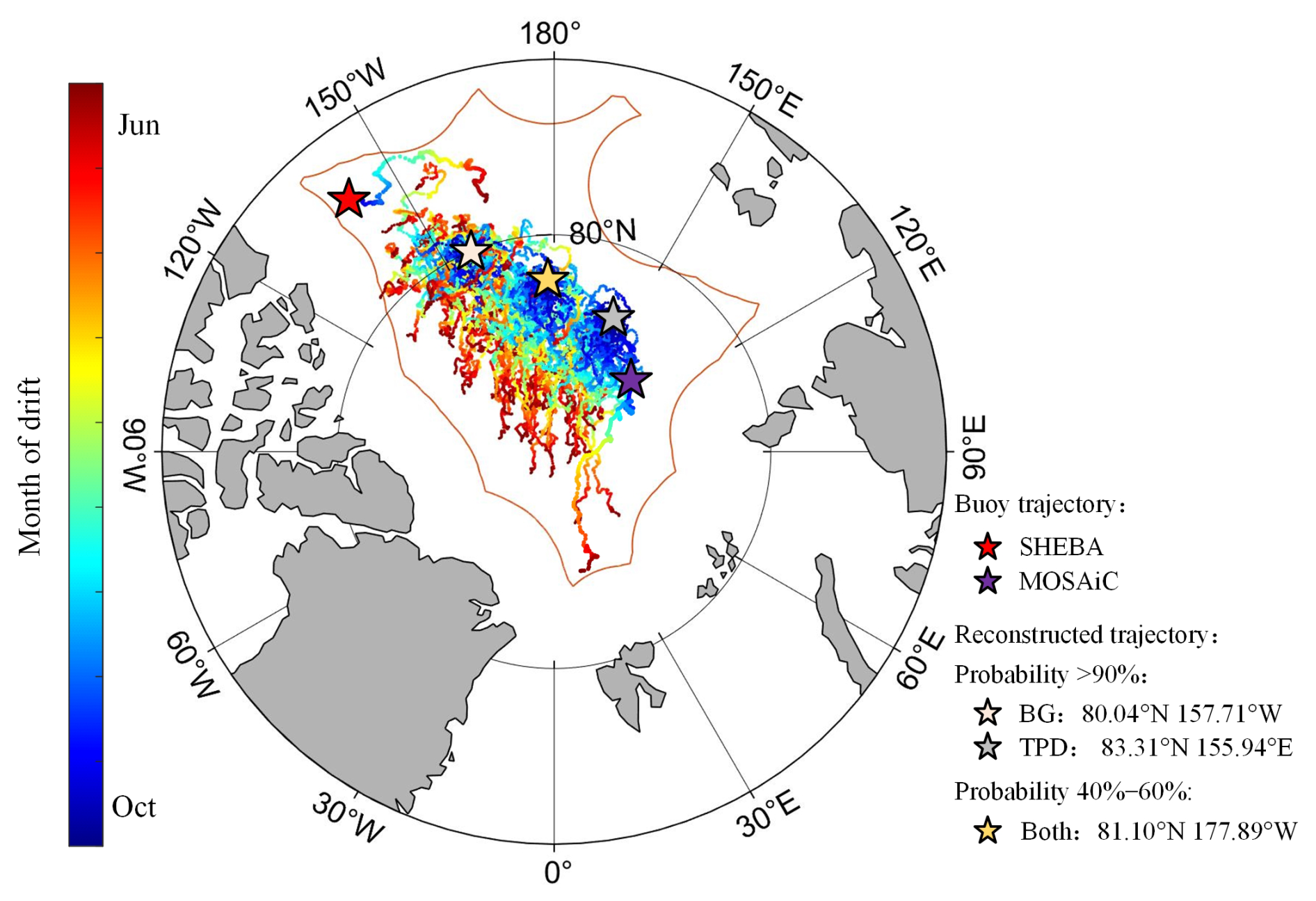
Figure 3 Reconstructed 9-month sea ice trajectories in 1979–2022, starting from 3 geometric centers of grid points with a greater than 90 % probability of reaching either the BG or TPD regions as well as that having an ambiguous destination, with a probability of 40 %–60 % of reaching both regions. For comparison, the partial drifting trajectories of the SHEBA and MOSAiC ice camps, which started from 3 October in 1997 and 2019 to 9 months after deployment, are also shown.

3 Results

3.1 Spatial distribution of the effective starting points of reconstructed ice trajectories with 9-month ST

Using the reconstructed ice trajectories for each ice season from 1979 to 2022, the influence of the specific starting point on the ST and its destination is assessed here. The results reveal that the effective probabilities (the ratio between the effective years to all study years from 1979 to 2022) of starting points with reconstructed ice trajectories having a sufficient ST of no less than 9 months ranged from 9.1 % to 90.9 %. Drifting from the region close to north of the East Siberian and Laptev seas (centered at about 82° N and 160° E) shows a relatively higher probability over the 44 years compared to other regions, generally exceeding 75 %. The likelihood of sea ice drifting into EEZs or beyond the ice zone increased when the starting point approached the corners of the rectangular study region, particularly in the downstream region of the TPD, where the probability is notably less than 20.0 %. The eligible points shown in Fig. 4b indicate the locations (with a size of 7.0 × 10⁵ km²) that served as starting points for reconstructed trajectories with ST ≥9 months in at least 33 years (or 75 %) from 1979 to 2022. Among them, the blue dots represent moderate recommendation zones in the central Arctic Ocean for ice camp or buoy deployment, where Lagrangian observations have a 75 %–85 % probability of lasting sufficiently long, with these zones occupying 80.4 % of the eligible area. The red dots, on the other hand, having a probability of >85 %, are high recommendation zones, occupying 19.6 % of the eligible area.

The probabilities of reconstructed ice trajectories terminating in the BG or TPD regions during the study period are illustrated in Fig. 4c–d. From 1979 to 2022, as expected, the ice floes that tend to drift to the BG region (Fig. 4c) mainly originate from the southwest part of the defined rectangular area; while the ice floes that tend to drift to the TPD region (Fig. 4d) mainly originate from the northeast part of the rectangular area. However, there is also a large overlapping area between these two regions, and the probability magnitudes exhibit a regular regional variability pattern for the specific regions. This suggests that the location of the starting point has a crucial influence on the subsequent ice advection. Thus, the deployment areas of the ice camp or buoy would determine their drift trajectory and final destination to a high degree. The number of eligible starting points, whose reconstructed trajectories reached the TPD region with a ST of no less than 9 months in over 75 % of the years in the 44-year study period, was 2.2 times that of starting points that reached the BG region. This indicates that sea ice originating from eligible starting points is more likely to reach the TPD region. For the ice floes originating from the junction zone between the BG and TPD regions (yellow strip in Fig. 4b), defined using the climatological SIM field, the probability of reconstructed ice trajectories reaching these two regions ranges from 42.5 % to 52.5 %, without any obvious regional tendency for ice advection destination.

Noting the significant shift in the physical nature of Arctic sea ice after 2007 (Sumata et al., 2023), we further calculated the probability distribution of starting points whose reconstructed ice trajectories terminated at the BG or TPD regions for the sub-periods prior to and after 2007, as shown in Fig. 5. The probabilities of starting points having a sufficient ST of no less than 9 months ranged between 14.3 % and 92.9 % in 1979–2006, which changed to 7.3 %–87.5 % subsequently, indicating a greater variability after 2007 (Fig. 5a–b). The size of the ideal deployment area (red and blue dots), with a probability >75 % of reaching the regions in Fig. 5c–d, was reduced obviously in 2007–2022 (2.1 × 10⁵ km²) by 81.3 % compared to that derived for 1979–2006 (11.2 × 10⁵ km²). In particular, the area of high recommendation zones (red dots) shrunk from 6.9 × 10⁵ km² in 1979–2006 to an almost negligible area of 1.1 × 10⁴ km² in 2007–2022. Such a conspicuous reduction in moderate and high recommendation zones suggests that the deployment of ice camps or buoys to obtain sufficiently long Lagrangian drift observations in the central Arctic Ocean has become more challenging as sea ice decreases.

The spatial distributions of the probabilities of reaching the BG and TPD regions in the two sub-periods – prior to or after 2007 – are similar to those for the whole study period (Fig. 5e–h). The spatial proportions of starting points with a >75 % probability of reaching the two regions varied slightly for the two sub-periods, with changes ranging from 0.7 % to 4.8 % relative to the full period. This suggests the destination of ice floe advection is relatively stable, which is mainly associated with the Arctic sea ice circulation patterns (detailed analysis will be provided in Sect. 4.2).

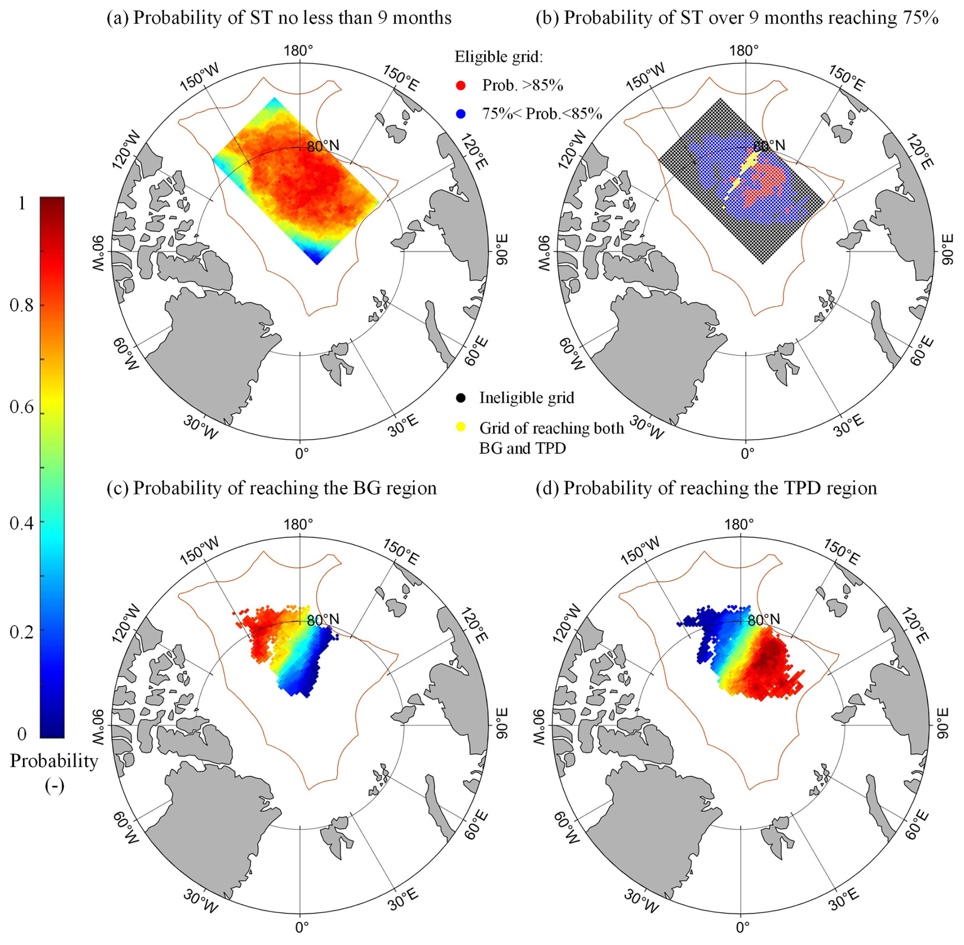
Figure 4 Spatial distribution of the probability that sea ice drifting from a defined grid point satisfies the following conditions in 1979–2022: (a) the ST within the central Arctic Ocean is no less than 9 months; (b) the region where the probability of the ST being over 9 months reaches 75 % (red and blue dot); also shown is the junction zone between the BG and TPD regions (yellow strip), defined using the climatological SIM field; (c–d the probabilities of reconstructed trajectories reaching the (c) BG or (d) TPD region.

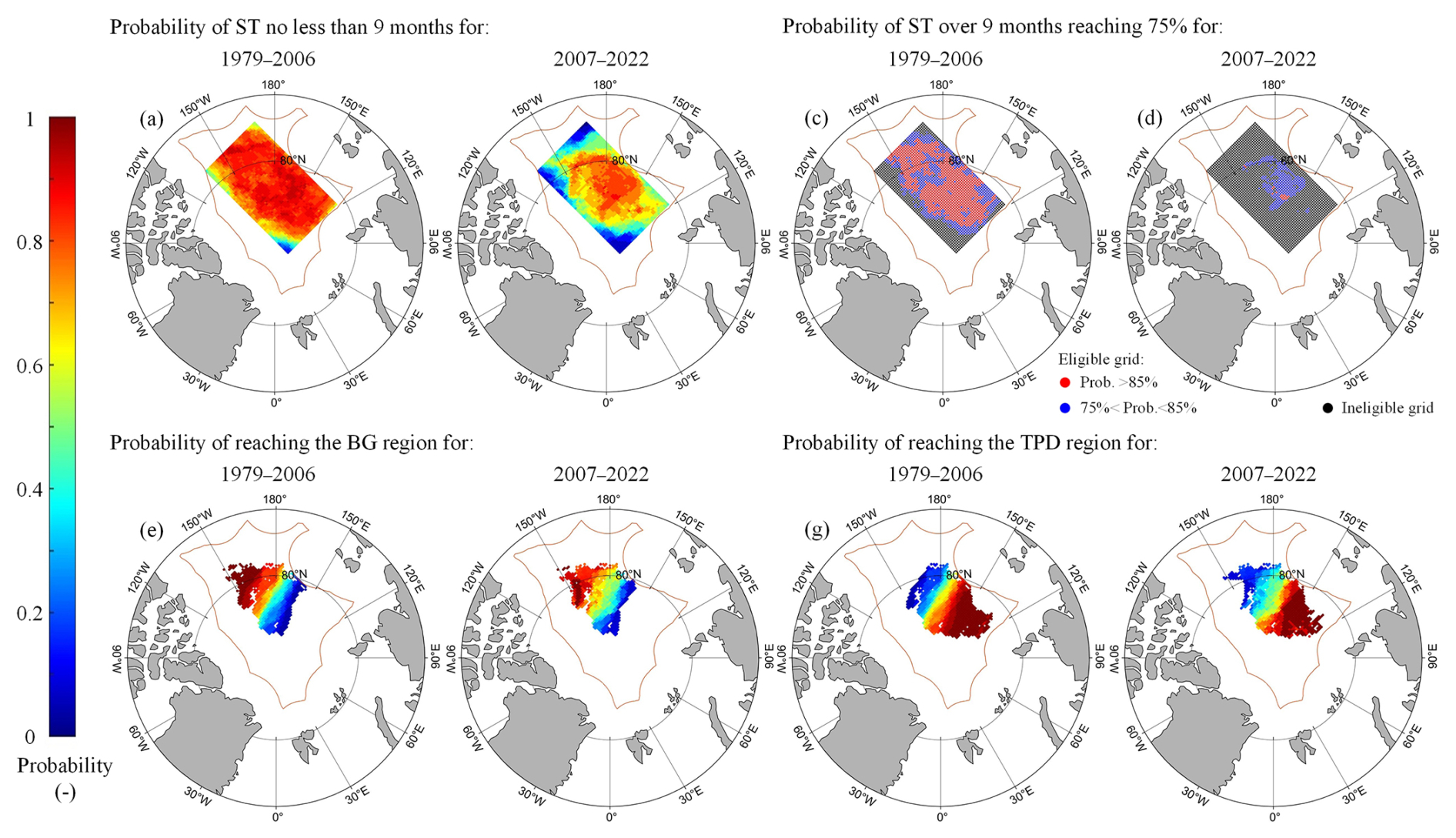
Figure 5 Spatial distribution of the probability that sea ice drifting from a defined grid point in the two sub-periods of 1979–2006 and 2007–2022 under the following conditions: (a–b) probability of ST of no less than 9 months; (c–d) the region where the probability of ST being over 9 months reaches 75 % (red and blue dot); and probability of reaching the (e–f) BG or (g–h) TPD region.

3.2 Changes in atmospheric thermodynamic and dynamic forcing along the trajectories

Sea ice thermodynamic growth is regulated by both atmospheric and oceanic forcing. Since the oceanic heat flux underneath the ice is relatively weak during the freezing season (Lei et al., 2022), near-surface air temperature could be considered as the most decisive parameter regulating ice growth and is a major atmospheric forcing factor for the sea ice growth analysis model (Leppäranta, 1993). In 1979–2022, the average air temperature along ice trajectories was higher in the TPD region (−17.6 °C) than in the BG region (−18.2 °C), with a slightly higher increasing trend (0.096 °C yr⁻¹) than that in the BG region (0.082 °C yr⁻¹). This is consistent with enhanced warming in the Atlantic sector of the Arctic Ocean (Rantanen et al., 2022). Despite significant increases in air temperature in both regions, the occurrence of extremely high air temperatures, exceeding the 90th percentile of the daily mean from 1979 to 2022, also defined as hot days by Vautard et al. (2013), did not change significantly. They occurred mainly in June, with similar frequencies in both regions (BG: 7.3 %–12.4 %, TPD: 6.6 %–13.2 %). This implies that extreme events with high near-surface air temperatures are largely concentrated in the initial stage of ice melting (Markus et al., 2009). These events are often accompanied by rainfall (e.g., Robinson et al., 2021). The average precipitation along the trajectories increased significantly in both regions (BG: 0.13 mm, TPD: 0.10 mm, P<0.05) in 1979–2022, but a significant increase in accumulated snowfall was only observed in the BG region (0.50 mm w.e. yr⁻¹, P<0.05). The TPD region is more susceptible to a shift in precipitation from snowfall to rainfall due to warmer conditions (Cohen et al., 2020), resulting in an insignificant change in snowfall. Especially in late spring and summer, increased precipitation in the form of rain accelerates the melting of the sea ice surface, promoting melt ponds formation (e.g., Feng et al., 2021) and triggering positive albedo feedbacks (e.g., Goosse et al., 2018).

To further investigate the potential effect of near-surface temperatures on sea ice melting or freezing, we calculated the FDD and TDD along the trajectories in 1979–2022. The BG region had higher a FDD than the TPD region, indicating warmer conditions during the freezing season in the TPD region despite its higher latitude (Fig. 6). FDD in the BG region showed a significant decreasing trend (P<0.05), slightly larger than that in the TPD region. However, the magnitude of TDD along the trajectories reaching both regions (BG and TPD) did not differ considerably, and it did not reveal a clear trend due to the insignificant summer warming trend in the Arctic Ocean. In winter, the average surface net longwave radiative flux along trajectories in the TPD region was upward, indicating heat loss from the sea ice–ocean system to the low atmosphere. The peak of the probability distribution of its absolute value decreased from about 57.5 W m⁻² prior to 2007 to about 52.5 W m⁻² after 2007. However, such a shift in the BG region was relatively weak from about 52.5 to about 50.0 W m⁻² (Fig. 7). This indicates that the weakened radiational cooling effect from the surface in the TPD region under clear-sky conditions was more pronounced compared to that in the BG region, which also can be attributed to the difference in winter warming trends between the two regions. Moreover, the frequency of net longwave radiation flux under opaque cloudy conditions in winter, having a typical value of >−10 W m⁻² (Graham et al., 2017), increased from 3.6 % in 1979–2006 to 4.3 % in 2007–2022 in the TPD region, while it decreased from 4.3 % to 4.2 % in the BG region. This is likely due to enhanced cyclonic activity in the Atlantic sector of the Arctic Ocean (e.g., Zhang et al., 2023).

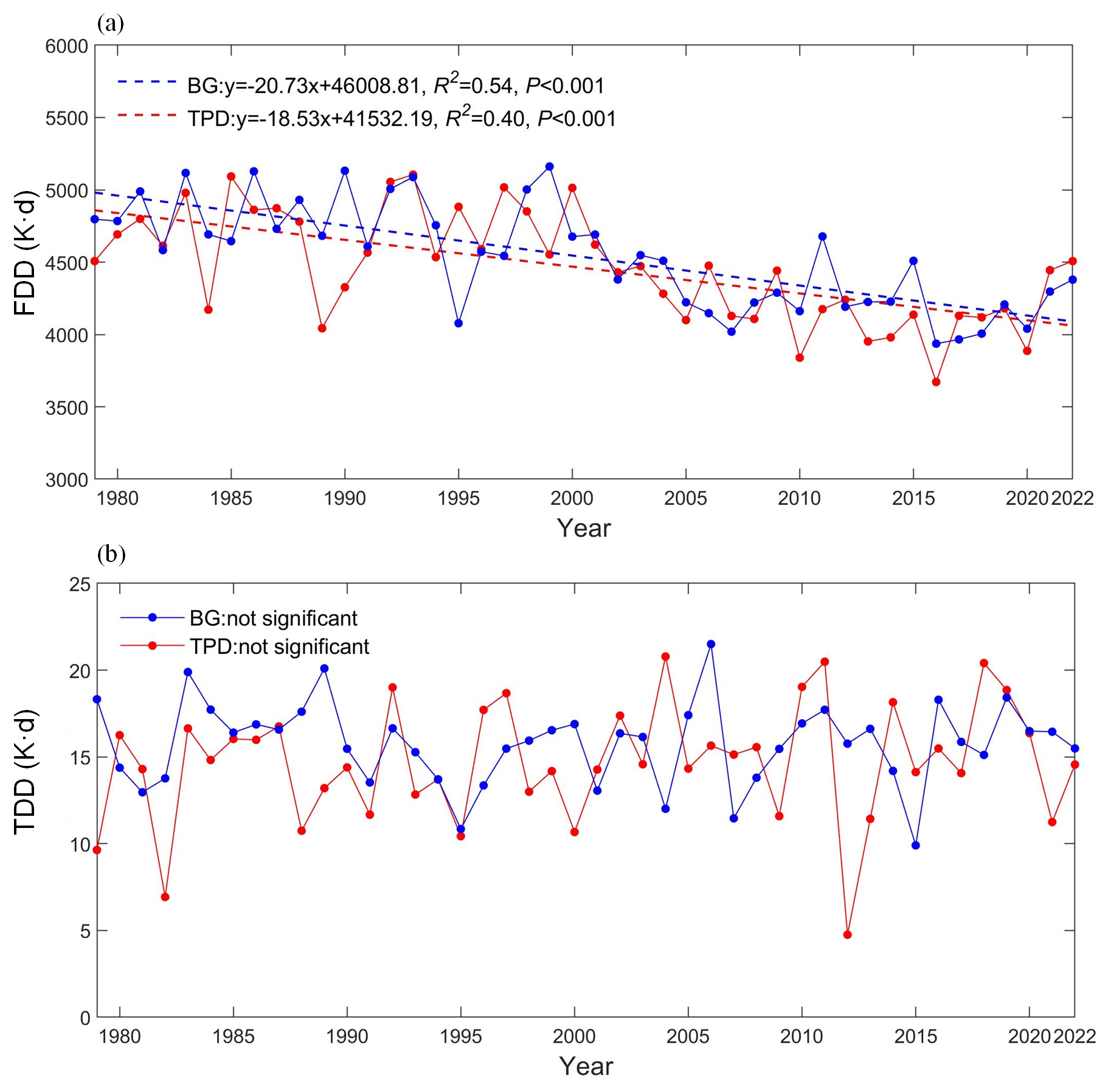
Figure 6 Changes in (a) FDD and (b) TDD during October to June in the two regions from 1979 to 2022.

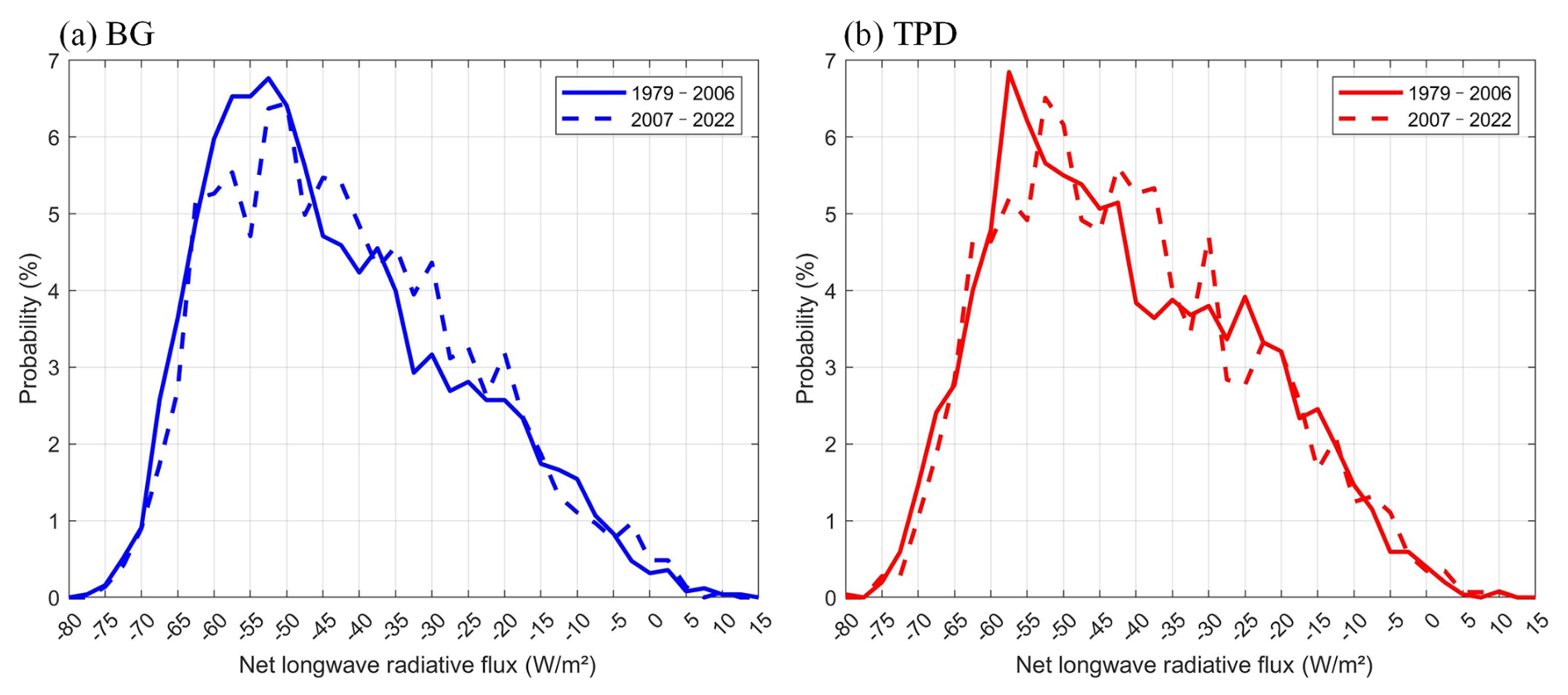
Figure 7 Probability distribution of the winter surface net longwave radiative flux along the trajectories in the BG and TPD regions for two sub-periods (1979–2006 and 2007–2022), with negative values denoting the upward flux from the surface.

The dynamic response of sea ice to wind forcing can be characterized using the ice–wind speed ratio (Herman and Glowacki, 2012). The seasonal average ice–wind speed ratio along the ice trajectories was largest in autumn (TPD: 1.55 %, BG: 1.52 %), which may be due to the relatively weak sea ice consolidation at that time (e.g., Lund-Hansen et al., 2020). Note that the ice–wind speed ratio is slightly lower than those obtained from buoy observations close to the North Pole by Haller et al. (2014), as the remote sensing SIM product typically underestimates SIM speeds due to the low temporal resolution (Gui et al., 2020). This ratio is also overall lower than the typical values in free-drift analytical solutions (Leppäranta, 2011), likely because higher SIC increases internal ice stress, enhancing resistance against SIM and reducing the sea ice response to wind forcing. Since 2007, the seasonal average ice–wind speed ratio in the BG region increased to 1.6 ± 0.3 % for the autumn, winter, and spring seasons, exceeding the TPD region by about 10.0 %. This indicates the ongoing enhancement of the dynamic response of sea ice to wind forcing in the BG region, linked to the replacement of thick multi-year ice by thin seasonal ice (Babb et al., 2023). Therefore, SHEBA campaign data (e.g., Lindsay, 2002) are no longer representative of the current ice state in the BG region.

4 Discussions

4.1 Assessment of reconstructed sea ice drift trajectories

To validate the reliability of the ice trajectory reconstruction method using the remote sensing SIM product, we used data from 16 buoys in the BG and TPD regions each (Table A1). Within the initial 100 d, most misalignment distances were less than 50 km (Fig. 8a), with RMSEs of 50.9 km. However, the reconstructed trajectories of 5 buoys were misaligned with the actual buoy trajectories by a relatively large distance (146.3–173.0 km after 100 d), likely due to the complex wind conditions at the early drifting stage of these buoys. These buoys experienced relatively high wind speeds (6.8 ± 2.7 m s⁻¹) in the first 10 d, with over 60.0 % of the days exceeding 6.0 m s⁻¹, which is higher than the climatological average since 1979 (5.6 ± 0.4 m s⁻¹). Conversely, wind speeds in the initial 10 d in our reconstructed trajectories in the BG and TPD regions over the 44-year period are mainly concentrated in the range up to 6.0 m s⁻¹ (>58.0 %), with modal wind speeds ranging from 4 to 5 m s⁻¹ (Fig. A1). This indicates that most reconstructed trajectories in this study did not experience strong wind conditions that could affect the accuracy.

Excluding the 5 buoys with complex initial wind conditions, the average misalignment distances between the reconstructed trajectories and the buoy trajectories (10 cases) after 9 months are 59.0 ± 41.4 km (about 2.5 pixels of ice motion product), and the RMSE is 68.6 km. The mean Fréchet distance was 89.6 km, the cosine similarities were all above 0.92, and the average endpoint Euclidean distance was 114.4 ± 87.5 km. This high geometric similarity ensures accurate advection direction and destination of the reconstructed trajectories. Regionally, there is a better reconstruction performance in the BG region than that in the TPD region. After 9 months, the average misalignment distance in the BG region (3 cases) is about 23.0 km, which is 30.9 % of that in the TPD region (7 cases), and the Fréchet distance is about 55.5 km, which is 48.1 % of that in the TPD region, consistent with the visual comparison of drift trajectories shown in Fig. 8b. This may be due to the larger SIM speed and its meridional gradient in the TPD region, especially in the southern region. All the reconstructed trajectories in the TPD region terminate at a further northward location compared to the corresponding buoy trajectories. This leads to a relatively ambiguous estimate of the effective duration of ice trajectories in the TPD region. However, we estimate this uncertainty to be approximately 1.6 % (or 4.3 d) compared with the buoy measurement, which looks trivial.

In addition, the semi-Lagrangian method has been proposed, which combines the Lagrangian and Eulerian aspects to reconstruct ice trajectories using a time-stepping procedure (Sagawa and Yamaguchi, 2006). Therefore, we compared the reconstructed trajectories obtained using the Lagrangian and semi-Lagrangian methods. For two starting points with >90 % probability of reaching the BG and TPD regions, the reconstructed trajectories using the two methods showed high similarity, with Fréchet distances of 8.3 km, average cosine similarity of above 0.99, and average misalignment distances of 3.5 ± 1.6 km in the BG region and 2.5 ± 1.2 km in the TPD region, respectively. However, relative to the validation data measured by 30 buoys, the semi-Lagrangian method exhibited larger errors compared to the Lagrangian method used in this study. The endpoint distances between the trajectories reconstructed using the semi-Lagrangian method and the actual buoy trajectories after 9 months (10 cases) were 118.6 ± 88.2 km, with misalignment distances of 61.1 ± 40.9 km, RMSEs of 70.8 km, Fréchet distances of 90.1 km, and cosine similarities all above 0.92. These statistical matrices are larger than those obtained by the Lagrangian method by 3.67 %, 3.56 %, 3.21 %, and 0.56 %, with comparable cosine similarities, respectively. This is likely because the semi-Lagrangian method does not directly track individual particles as precisely as the Lagrangian method (Subich et al., 2020), affecting its accuracy in reconstructing ice trajectories.

To further assess the reliability and the stability of the trajectories, we also conducted a closed loop examination by reconstructing backward ice drift trajectories from the endpoints of the original forward-reconstructed trajectories. This verification test required the reconstructed backward trajectories to return to their starting points after the same time period. Specifically, we initiated backward reconstructions from hotspot regions, i.e., regions where sea ice is more likely to reach and persist (defined using a density-based clustering method with a 75 % probability of the ST being >9 months in 1979–2022) at the endpoints of the forward trajectories. Consequently, 66.3 % of backward trajectories were projected to return to recommended regions, with 49.2 % and 17.1 % reaching the moderate and high recommendation zones, respectively (Fig. 9). This suggests that the recommendation zones, as a source area for sea ice, have stable paths. This closed calibration testing also demonstrates the high confidence in the method used to reconstruct ice trajectories.

To test the robustness of the duration estimate, we assessed the impact of year, starting position, and interpolation method on the duration, using the starting points of the trajectories reaching the BG or TPD regions with over 90 % probability as an example. The results showed that the standard deviation of duration in 1979–2022 amounted to 76.0 d; this standard deviation decreases to 20.7 d in 2007–2022, which corresponds to 7.2 % of the mean duration. It should be noted that this study mainly focuses on the mean duration characteristics at the climate scale. The difference in mean duration due to a starting position offset (±10 km) and the results obtained for the starting position accounts for about 1.1 %. Further, the mean duration obtained from the ice trajectories reconstructed with the nearest neighbor interpolation differs from the results obtained using the bilinear interpolation by an average of 7.6 %. This proves that small changes in the initial coordinates and the interpolation method barely affect the reliability of the duration estimate.

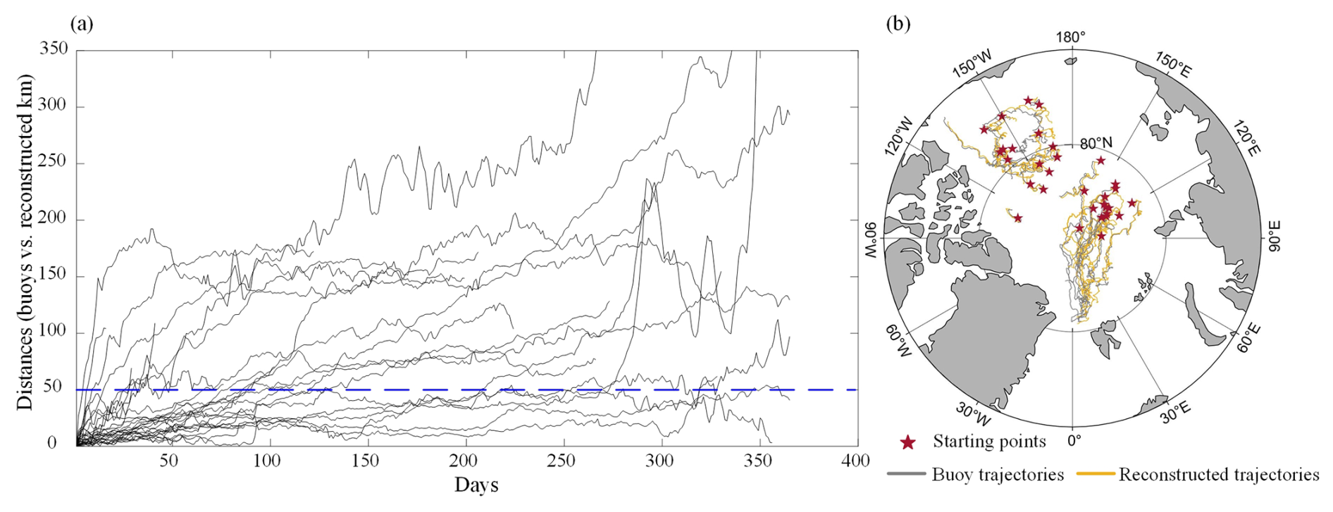
Figure 8 Comparison of reconstructed ice trajectories with buoy trajectories: (a) misalignment distances over time for trajectory pairs; (b) trajectory pairs from the deployment site of buoys.

Figure 9 Spatial distribution of endpoints of forward- and backward- reconstructed trajectories: (a) forward trajectory endpoints and hotspot regions; (b) endpoints of backward-reconstructed trajectories from hotspot regions.

4.2 Links of endpoints of ice trajectories to atmospheric circulation patterns

Based on three scenarios for ice trajectory endpoints, i.e., >90 % probability of reaching the BG or TPD regions and 40 %–60 % probability of reaching either region, we explored the links between the endpoints of ice trajectories to atmospheric circulation patterns (Table 1). We also analyzed the statistical relationship (Table 2) between the distance from the trajectory endpoints to Fram Strait (80° N) for the ice trajectories reaching the TPD region and atmospheric circulation indices, which allows exploring the potential mechanisms by which atmospheric circulation patterns affect sea ice outflow from the central Arctic Ocean.

For ice trajectories reaching the TPD region, autumn CAI and DA showed stronger correlations with the endpoint latitude after 9 months (R²: 21.8 % and 32.5 %, P<0.05) and with the distance between the endpoint of the ice trajectory after 9 months and the Fram Strait (R²: 21.8 % and 32.5 %, P<0.05) than BH. This is due to the fact that these indices directly modulate meridional wind forcing, i.e., their positive phases enhance transpolar drift by intensifying southerly winds across the TPD region (Wu et al., 2006; Vihma et al., 2012). In contrast, BH primarily affects the longitudes of the ice trajectories through zonal adjustments of the TPD pathway. When the BH index is positive, the BG squeezes the axis alignment of the TPD eastward, lengthening the distance that ice advects along the TPD toward the Fram Strait. This mechanistic difference explains why, in the TPD region, CAI is associated with latitudinal changes in ice drift trajectories, while BH is associated with longitudinal changes. Therefore, it is necessary to take the autumn CAI and DA index into consideration for predicting the subsequent trajectories of ice floes as well as that of the buoy or camp deployed on it in the TPD region.

For the ice trajectories reaching the BG region, although sea ice circulation in the BG region is driven by anticyclonic wind stress curl associated with a positive BH index (Proshutinsky et al., 2002), BH was not more effective in explaining the location of the ice drift endpoints in this region than other indices. This may be because the influence of BH on ice advection in this region is susceptible to interference from other atmospheric circulation patterns, in particular, the DA and the associated meridional wind anomalies (e.g., Wang et al., 2009). The weaker latitudinal than longitudinal correlations (R²: 9.5 % and 19.1 %, P<0.05) between the autumn CAI and DA and the endpoints after 9 months reflect the fact that the BG region can suppress meridional transport because sea ice motion in this region is mainly driven by anticyclonic circulation. Moreover, for sea ice that has the potential to reach both BG and TPD regions, all autumn atmospheric circulation indices showed significant explanatory power for the latitude of the endpoint and its distance to the Fram Strait after 9 months (P<0.05).

Since atmospheric circulation patterns in autumn, during the initial stage of ice drift in autumn, especially for the CAI and DA, had a strong influence on the endpoints of ice trajectories after 9 months in both the BG and the TPD regions, we further analyzed scenarios where these indices exhibited extreme positive (negative) anomalies, defined as a value higher (lower) than the 1979–2022 climatology by one standard deviation (Fig. 10). When CAI and DA are at extreme positive (negative) phases, the spatial proportions of starting points with a 9-month ST threshold for more than 75 % years are 75.2 % (46.3 %) and 86.0 % (44.1 %), respectively, which are greater (less) than the spatial proportions obtained from the mean field in 1979–2022 (48.6 % as shown in Fig. 2). This suggests that the extreme scenarios of the autumn CAI and DA indices have a pronounced modulating effect on the ideal deployment areas for Lagrangian observations, with a wider range of ideal areas at their extreme positive phases. Under extremely positive phases of CAI and DA, the preferred area of deployment tends to extend to the Chukchi Sea and the Canada Basin, while at the negative phase, it extends to the northern Laptev Sea. However, the extreme positive phase of the autumn CAI is associated with only a trivial increase (by 2.2 %) in the spatial proportion of points with >75 % probability of reaching the TPD region compared to the average state over 44 years. The extreme negative phase of the autumn DA, on the other hand, significantly increases the probability of trajectories reaching the BG region, and the spatial proportion >75 % is 1.5 times that obtained from the whole study period.

Table 1 Coefficient of determination (R²) between the atmospheric circulation indices and the location (longitude/latitude) of the sea ice trajectory endpoint after 9 months in 1979–2022.

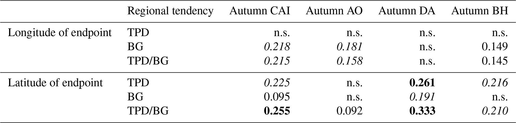
Note: Significance levels are P<0.001 (bold), P<0.01 (italic) and P<0.05 (plain); n.s. denotes insignificant result at the 0.05 level.

Table 2 The coefficient of determination (R²) of autumn atmospheric circulation indices for the distance between the sea ice trajectory endpoint after 9 months and the Fram Strait in 1979–2022.

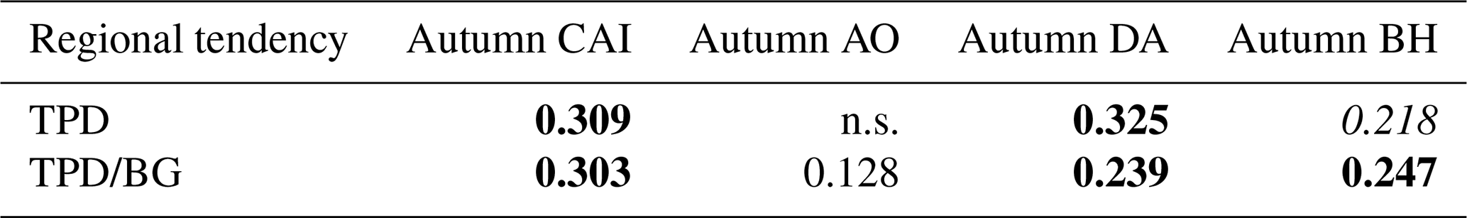
Note: Significance levels are P<0.001 (bold), P<0.01 (italic) and P<0.05 (plain); n.s. denotes an insignificant result at the 0.05 level.

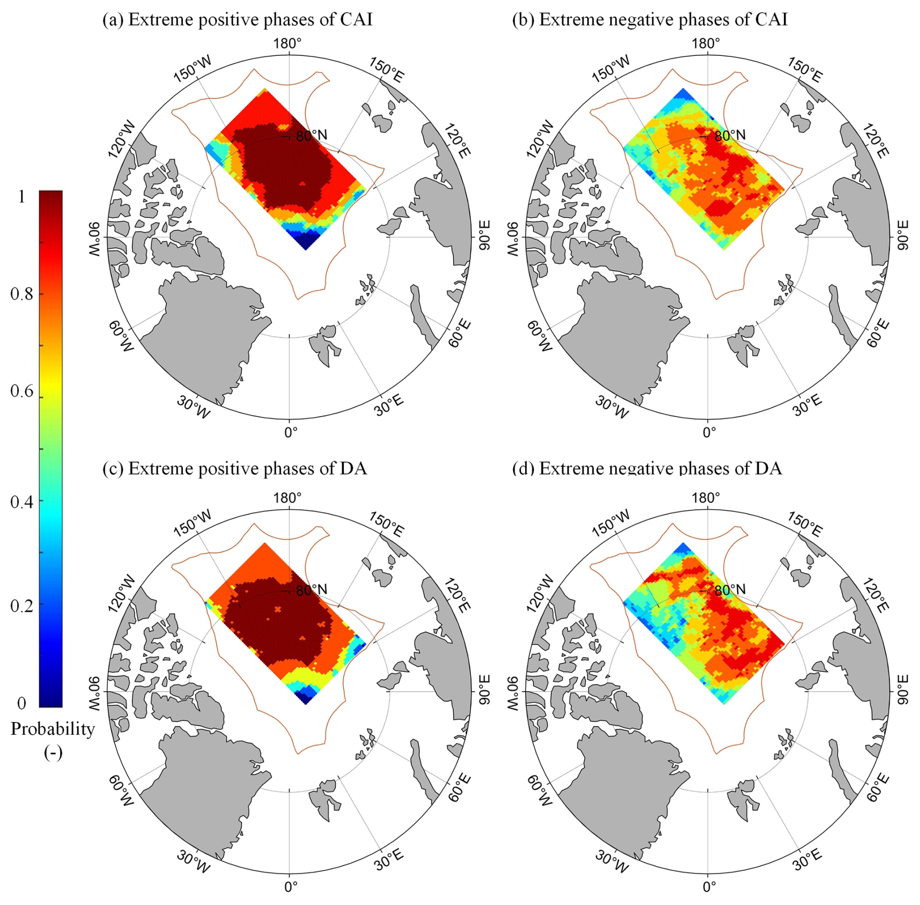
Figure 10 Spatial distribution of the probability that the ST of sea ice drifting from a defined grid point is no less than 9 months at the extreme positive and negative phases of the autumn CAI and DA for 1979–2022.

4.3 Impact of the EEZ boundary and deployment time on the ST of ice trajectories

The ST of reconstructed ice drift trajectories, or potential Lagrangian observations based on ice camps or buoys, is limited to a great extent by the EEZ boundary. To quantitatively evaluate the impact of the EEZ boundary, we hypothesized that enhanced international cooperation would be desirable to reduce the impact of geopolitical boundaries on this type of observation, and identified the ideal deployment areas for Lagrangian observations under this scenario. We found that without the limitation of the EEZ boundary, the probability of ST exceeding 9 months for ice trajectories reconstructed from all grids in the rectangular study region ranged from 45.5 % to 90.9 % between 1979 and 2022. The spatial range of probabilities >75 % (i.e., 33 years) for the ST threshold of 9 months extended to 83.7 % of the whole rectangular study region,which was much larger than the 48.6 % with the limitation of the EEZ boundary. Disregarding the EEZ boundary, the increase in eligible starting points with >75 % probability of reaching the regions is proportional to the used ST threshold (Table 3). Especially for the 10-month ST threshold, the eligible area increases by over 150 % compared to that with the limitation of the EEZ boundary. Disregarding the EEZ boundary, the increase in eligible starting points in the rectangular study region with >75 % probability of reaching the BG or TPD regions is also proportional to the ST threshold. Particularly for the 10-month ST, the number of eligible starting points reaching the BG or TPD regions increases by over 100 % when the limitation of the EEZ boundary is removed. For starting points with a close probability of reaching both BG and TPD regions, the spatial proportion of eligible starting points would instead be suppressed compared to estimates that account for the EEZ boundary. This is because these eligible starting points are primarily located at the junction of the BG and TPD regions and relatively far from the EEZ boundary.

For the period 1979–2022, the average Lagrangian observation duration in the rectangular study region disregarding the EEZ boundary is about 298.0 ± 25.7 d, which extends by about 34.3 d compared to observations that account for the EEZ boundary. Regionally, the Lagrangian observations located in the BG and TPD regions would be further extended by about 20.5 d (286.1 ± 128.1 d) and 5.0 d (298.3 ± 114.4 d), respectively. This suggests that the EEZ boundary has a slightly larger impact on the observation duration in the BG region compared to the TPD region, because the EEZ boundary downstream to TPD is overall close to the marginal ice zone. Spatially, for sea ice reaching the BG region, the added eligible starting points are located in the southern part of the BG, as shown in Fig. 11. Sea ice originating from these locations might be more strongly affected by the clockwise ice circulation of the BG and cross beyond the EEZ boundary in the south more easily. For the ice trajectories reaching the TPD region, the added eligible starting points are located in the south of the study region or in the sector facing the Fram Strait. Sea ice originating from these areas might have been advected more rapidly to cross the EEZ boundary in the Atlantic sector.

Table 3 Increased spatial percentage in eligible starting points without considering EEZ constraints compared to those estimated with the constraints.

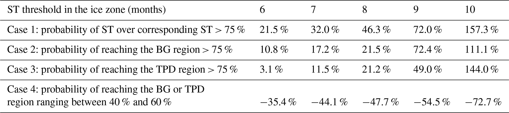
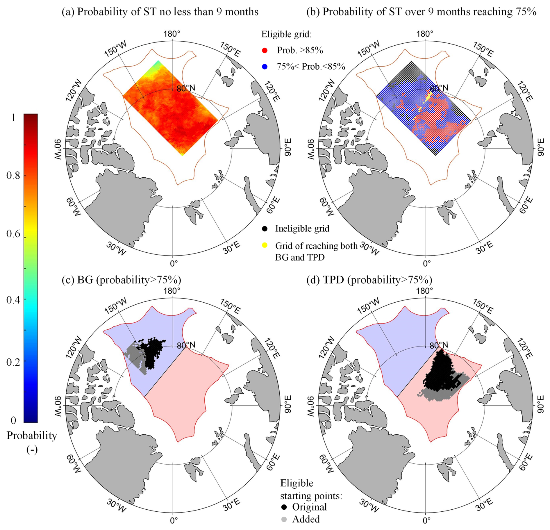
Figure 11 Assuming that the EEZ boundary constraints are not considered in 1979–2022: (a) spatial distribution of the probability of ST in the ice region being no less than 9 months; (b) the region where the probability of ST being over 9 months reaches 75 % (red and blue dot); also shown is the junction zone between the BG and TPD regions (yellow strip); and (c–d) the added eligible starting points (gray) with >75 % probability of reaching the BG or TPD regions, compared to those estimated with the EEZ constraints (black).

To further assess the influence of the setup time of the ice camp or buoy on the potential duration of subsequent observations, using the starting points of trajectories reaching the BG or TPD regions with over 90 % probability (Fig. 3), we calculated the duration with the deployment date ranging from 15 August to 1 November (Fig. 12). The mean duration of Lagrangian observations in the two regions decreases gradually from 296.1 ± 11.8 d for the deployment on 15 August to 279.9 ± 17.1 d for the deployment on 1 November. Although delaying the deployment of ice camps or buoys on ice floes to 15 August may result in longer observation times, approximately by 10.0 d, compared to deployment on 1 October, we argue that it is more appropriate to deploy in early October if the logistics allows, as there is often a risk that the ice holes drilled for equipment deployment are hard to refreeze, and the risk of floe fragmentation would increase by the end of the ice melt season in August and September. In these situations, the equipment is prone to collapse, causing observation interruptions. As expected, the duration in both regions is longer when EEZ constraints are disregarded. Even in the BG region, which has a shorter duration of observation compared to the TPD region, the potential duration for Lagrangian observations is estimated to reach 255.4 d with the EEZ constraints and 283.3 d without the EEZ constraints, respectively, when the ice camp or buoy is deployed on 1 November. This suggests that deploying buoys or camps on ice floes in the central Arctic Ocean, even by the end of October, given EEZ constraints, is still able to guarantee a observation duration of at least 8 months. Furthermore, the influence of EEZ constraints on potential Lagrangian observation duration would gradually strengthen with later deployment dates.

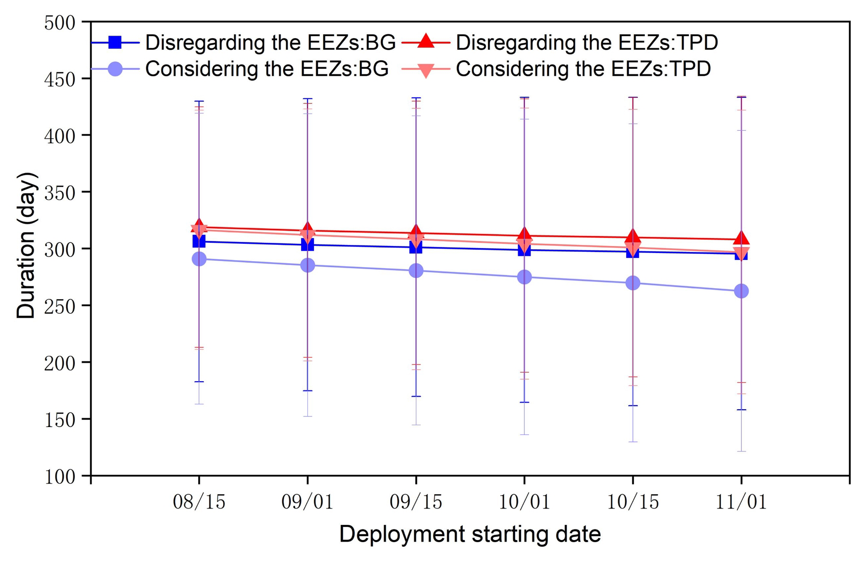
Figure 12 Changes in the mean duration of Lagrangian observations in 1979–2022 for various deployment dates, using starting points that reached the BG or TPD regions with over 90 % probability, under both scenarios: with or without the EEZ constraints.

5 Conclusions

For a rectangular study region defined in the central Arctic Ocean that excludes EEZs, we reconstructed sea ice trajectories for 1979–2022 and determined ideal deployment areas for subsequent Lagrangian observations with an expected duration. Based on this, regional differences in atmospheric conditions along the trajectories were assessed. Subsequently, we explored how atmospheric circulation patterns regulate sea ice advection and how EEZ boundary constraints and deployment time influence the duration of sustained Lagrangian observation.

The deployment of Lagrangian observations at locations centered around 82° N and 160° E, near north of the East Siberian and Laptev seas can ensure at least 9 months of drifting observation time. The probabilities of remaining in the central Arctic ice region during the 44-year study period ranges from 75.0 % to 90.9 %, with mainly moderate recommendation zones (75 %–85 %) with a spatial proportion of 80.4 % and a small proportion of high recommendation zones (>85 %). Ice floes originating from this area of 7.0 × 10⁵ km² are more likely to reach the TPD region.

There are obvious regional differences in atmospheric and sea ice conditions during ice drifting between the BG and TPD regions. Near-surface (2 m) air temperatures in both regions show a significant warming trend in 1979–2022, with a higher increasing rate in the TPD region due to its proximity to the Atlantic sector of the Arctic Ocean. The significant decrease in FDD in the BG and TPD regions suggests that sea ice is experiencing warmer conditions during the freezing season in recent years. Lagrangian observations in the TPD region would experience an increase of 19.4 % in days of cloud opacity during winters in 1979–2022 by 19.4 %, compared to in 1979–2006, because of more frequent cyclone activities in the TPD region in recent years. The observations in the TPD region in 1979–2006 experienced a relatively stronger dynamic response of sea ice to wind forcing, indicated by a higher ice–wind speed ratio than in the BG region. However, this response was enhanced in the BG region due to the larger loss of multiyear ice, especially in the south part of the BG region. Large-scale atmospheric circulation patterns at the early stage of ice drifting in autumn have a significant influence on the terminal location of ice trajectories. Thus, compared to the 1979–2022 average, the extreme positive phases of the CAI and DA indices in autumn expanded the ideal deployment area to the Chukchi Sea and the Canada Basin. On the contrary, at the extreme negative phase of these indices, it is preferred to expand to the northern Laptev Sea.

In addition to natural conditions, the EEZ boundary greatly constrains Lagrangian observations. The absence of these constraints would increase the number of eligible starting points in the study region. When we disregard EEZ boundary constraints, the eligible starting points with trajectories reaching the BG region expand southward, while for those reaching the TPD region, the starting points would expand in the areas facing the Fram Strait. Advancing the deployment start time to mid-August may result in a longer duration of Lagrangian observations, by 10.0 d compared to that obtained from deploying on 1 October. However, in order to reduce the risk of failure of observation instruments deployed on the floes, particularly in the later ice melt season, we consider deployments in October more appropriate for Lagrangian observations relying on ice floes in the central Arctic Ocean. Compared to buoy data, the reconstructed trajectories have high geometrical similarity and accuracy, validating our method. The reconstruction in the BG region is better than that of the TPD region. Meanwhile, the accuracy of the Lagrangian method for ice trajectory reconstruction is higher than that of the semi-Lagrangian method, and the high probability of closure of the reconstructed forward and backward trajectories indicates the high confidence of the reconstruction method.

In this study, the daily SIM product is the main data source used to reconstruct sea ice drift trajectories and evaluate the ST of Lagrangian observations relying on ice floes. We acknowledge that this is a primary evaluation, ignoring operational safety risks. The main challenges for the survival and continuous deployment of the specific devices deployed on Arctic ice floes include the breakage or compression of sea ice, the formation of melt ponds, the intrusion of polar bears, etc. As Arctic warming continues, the combined effects of accelerated melting and the limited replenishment of multi-year ice will eventually trigger the complete loss of multiyear ice and a shift to a seasonally ice-free Arctic Ocean (Babb et al., 2023). This change will increase the demands on ice floe–based observational campaigns and further emphasize the need for more adaptive observational techniques and equipment to cope with future extreme ice and atmospheric environments. Our work mainly supports site selection for the deployment of buoys and ice camps on ice floes. The preferred areas identified in this study require adaptable adjustments, associated with changes in Arctic sea ice in the future. From a practical perspective, on reaching the preferred deployment area, the specific conditions of the ice floe, such as ice thickness, floe size, and the distribution of ice ridges and melt ponds, need to be further surveyed using high resolution satellite remote sensing images and helicopters or ice-based measurements.

Appendix A

Table A1 Basic information on buoy data used for validating the reconstructed ice drift trajectories.

Note: buoys without specified types indicate that the IABP does not provide information on the buoy type.

Figure A1 Probability distribution of wind speed in the initial 10 d along the reconstructed trajectories in the BG and TPD regions in 1979–2022.