Modelling cold firn evolution at Colle Gnifetti, Swiss/Italian Alps

The existence of cold firn and ice within the European Alps provides an invaluable source of palaeoclimatic data with the capability to reveal the nature of anthropogenic forcing in western Europe over the preceding centuries. Unfortunately, continued atmospheric warming has initiated the thermal degradation of cold firn to that of a temperate firn facie, where infiltrating meltwater compromises this vital archive. However, there is currently limited knowledge regarding the transition of firn between these different thermal regimes. Here, we present the application of a modified version of the spatially distributed Coupled Snow and Ice Model in Python (COSIPY) to the high-altitude glacierised saddle of Colle Gnifetti (CG; 4452 m a.s.l.) of the Monte Rosa massif, Swiss/Italian Alps. Forced by an extensively quality-checked meteorological time series from the Capanna Margherita (CM) station, with a distributed accumulation model to represent the prevalent on-site wind-scouring patterns, the evolution of the cold firn's thermal regime is investigated between 2003 and 2023. At the saddle point (SP), our results show surface melt increasing at a rate of 0.53 cm w.e. yr⁻² – representing a doubling over the 21-year period. This influx of additional meltwater and the resulting latent heat release from refreezing at depth drive englacial warming at a rate of 0.051 °C yr⁻¹, comparable to in situ measurements. Since 1991, a measured warming of 1.5 °C (0.046 °C yr⁻¹) has been observed at 20 m depth with a strong inversion in the temperature gradient developing in the last decade through the 18–30 m depth range of the glacier – also partially reproduced by our model. In lower-altitude regions (∼ 4300 m a.s.l.), simulated warming is much greater than the local rate of atmospheric warming, resulting in a rapid transition from cold to temperate firn – potentially indicative of future conditions at the saddle point of Colle Gnifetti. However, simulated firn temperatures are particularly sensitive to the parameterisations for modelling albedo and preferential percolation in this cold-temperate transition area.

1 Introduction

Glaciers can be differentiated with respect to their thermal characteristics: those that exist permanently at negative temperatures below the depth of seasonal variation are referred to as “cold”, whilst those maintaining a temperature at the pressure melting point of ice are known as “temperate”. However, in practice, fully cold ice bodies are rare; most exist in a “hybrid” or “polythermal” state (Blatter and Hutter, 1991). In the European Alps, the formation of cold firn (the term used to describe the intermediate stage between snow and glacial ice) is limited to the high-altitude (⪆ 3500 m a.s.l.) accumulation areas of polythermal glaciers (Lüthi and Funk, 2001b; Suter and Hoelzle, 2002; Gilbert and Vincent, 2013; Gilbert et al., 2015); these can similarly be classified into zones of differing thermal regimes known as firn facies according to Shumskii (1955, 1964):

• the re-crystallisation zone, where the surface temperature never reaches the melting point and as such no surface melt occurs;

• the re-crystallisation–infiltration zone, where melt occurs but meltwater percolation is limited to the uppermost snow layers of the current accumulation year and does not penetrate into the firn layers beneath;

• the cold infiltration zone, where meltwater can percolate through several layers of annual firn but is either internally retained or refrozen;

• the temperate firn zone, where englacial temperatures at all depths tend to the melting point and meltwater can fully percolate through the firn.

Within the re-crystallisation and re-crystallisation–infiltration facies, the depositional stratigraphy of accumulated snow layers is not compromised by a significant infiltration of surface meltwater (Shumskii, 1964; Hoelzle et al., 2011). The glaciochemical analysis of these distinguishable annual layers of cold firn can reveal the historic variability in the climate and atmospheric composition (Oeschger et al., 1977; Wagenbach et al., 2012; Bohleber, 2019; Eichler et al., 2023). In western Europe, the retrieval of such ice cores has been indispensable due to their close proximity to a principal source of historic anthropogenic emissions (Jenk et al., 2009; Legrand et al., 2013). Unfortunately, climate change has initiated the thermal degradation of existing cold firn areas where the increasing infiltration of meltwater endangers the future longevity of these archives (Eichler et al., 2001; Gabrielli et al., 2010; Hoelzle et al., 2011). Ultimately, a gradual transition of cold to temperate firn is anticipated over time (Lüthi and Funk, 2001a; Gilbert et al., 2014). However, the monitoring of englacial temperature changes can itself be a vital indicator of a cold or polythermal glacier's response to current atmospheric warming (Hoelzle et al., 2011; Gilbert and Vincent, 2013). Unlike traditional glaciological measurements that focus on mass losses in the ablation zone, cold firn areas do not exhibit significant mass changes due to the retention and refreezing of meltwater; the additional energy instead manifests as an increase in englacial temperature (Haeberli and Beniston, 1998; Vincent et al., 2020).

Colle Gnifetti (CG), a high-altitude glacierised saddle in the Monte Rosa massif (Fig. 1), has been at the forefront of alpine cold firn research for half a century, possessing an extensive archive of climatological measurements. Unique to any other cold firn site in central Europe, the extremely low flow and accumulation rates at CG (minimum of 15 cm w.e. yr⁻¹; Bohleber et al., 2013), relatively large glacier thickness (average 100 m; Haeberli et al., 1988), and favourable topographic setting enable ice core dating up to the late Pleistocene (19.6 kyr BP) (Jenk et al., 2009; Wagenbach et al., 2012). Englacial temperatures have been measured at CG since 1977. Haeberli and Funk (1991) concluded that observed englacial temperatures derived from borehole measurements in 1982 remained near steady-state conditions with a limited influence of meltwater refreezing. However, subsequent measurements in 1995 revealed inflexions in the thermal profile at shallow depth and were interpreted by Lüthi and Funk (2001a) to indicate the onset of firn warming. Thereafter, Hoelzle et al. (2011) published further evidence of englacial warming at CG noting that areas beneath the saddle on the Grenzgletscher had already undergone a facie transition from a re-crystallisation–infiltration to a cold infiltration zone due to enhanced meltwater percolation.

Suter and Hoelzle (2002) conducted a large-scale fieldwork campaign across the wider Monte Rosa massif in 1999, with extensive borehole measurements aiming to determine the spatial extent of existing cold firn. Suter and Hoelzle (2002) noted strong firn temperature variation across the region, brought about by changes in insolation, accumulation, slope, and surface aspect. Further research included the analysis of surface energy exchanges from a temporary monitoring station at Seserjoch and the application of a basic time-dependent firn temperature model to estimate future englacial warming rates (Suter et al., 2001, 2004). Later, Buri (2013) applied the GEO-top hydrological model using meteorological data from the nearby automatic weather station (AWS) at the Capanna Margherita (CM) (operational since 2002); however, both these models were only applied on isolated point nodes as opposed to a fully distributed spatial domain. Recently, Licciulli et al. (2020) implemented a fully three-dimensional thermomechanically coupled model; however, their study focused more on ice rheology to support palaeoclimatic research and assumed no infiltration and release of latent energy from meltwater refreezing at depth within the firn.

In general, the application of physical firn models to CG is constrained by the complexity of representing the variability in accumulation. The exposed saddle is highly susceptible to extreme wind scouring of the snow surface that can even periodically lead to years with net mass ablation (Lüthi and Funk, 2001a; Wagenbach et al., 2012). However, this process can be counteracted by the melt-induced consolidation of the snowpack in the presence of strong insolation (Alean et al., 1983). Thus, snow accumulation has a strong summer bias and therefore conforms to the aspect-derived insolation gradient across the saddle, favouring the slopes of the Zumsteinspitze (Licciulli et al., 2020). Mattea et al. (2021) applied the spatially distributed, physically based energy balance firn model (EBFM) of van Pelt et al. (2012) to CG, using extensively quality-checked, high-resolution hourly meteorological data from the AWS CM between 2003 and 2018. Accumulation variability was modelled using a spatiotemporally variable precipitation input, as the single-dimensional model lacked a representation of lateral mass transfer processes. Mattea et al. (2021) investigated the evolution of firn temperatures and the dynamics of surface melt, reporting a pattern of increasing annual surface melt production – despite high inter-annual variability – perceived to be driving englacial warming at CG.

Here, we present the direct continuation of their research: the application of an alternative coupled energy balance and multi-layer subsurface firn model to CG, extending the simulation period by 5 years to investigate changes in the thermal regime up to the present day. We further refine the original study by introducing a new model spin-up with representative meteorological data from the early 20th century to improve the model initialisation conditions and by incorporating new physical processes, such as subsurface melting and penetrating shortwave radiation. Our results provide greater insight into the firn warming observed at CG during the 21st century and, in particular, a strong acceleration since 2015, driving an inversion in the near-surface thermal gradient.

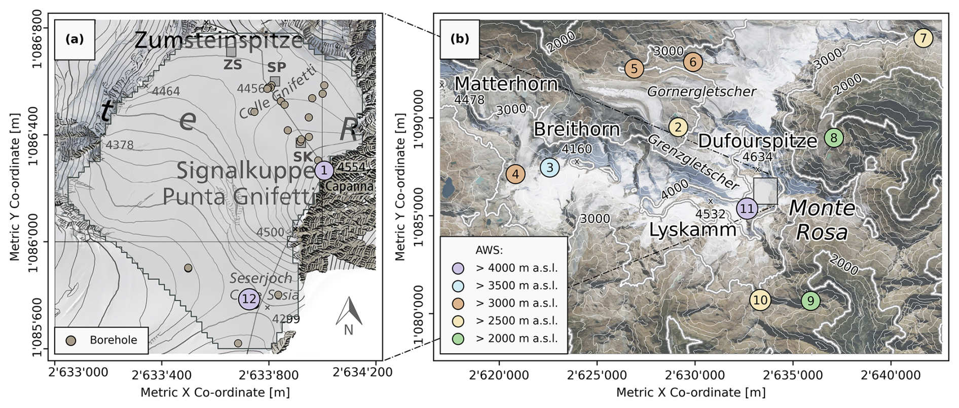
Figure 1 (a) Map of the study area at Colle Gnifetti showing key locations (ZS: Zumsteinspitze slope; SP: saddle point; SK: Signalkuppe slope) and borehole locations from which thermistor profiles and firn/ice cores were extracted at the site. (b) Overview map of the Monte Rosa region showing the location of the study area and the meteorological stations (AWS) listed in Table 1. Spatial co-ordinates are defined by EPSG 2056 (Metric Swiss CH1903+/LV95). Topographic map and orthoimage sources: Swisstopo (2017, 2023) and Vexcel Imagery (2022). Elevation contours are derived from the Copernicus 30 m digital elevation model (DEM) product (Copernicus, 2024).

ARPA Piemonte (2024)MeteoSwiss (2024)DTN (2024)MeteoAM (2020)MeteoSwiss (2024)Hoelzle et al. (2022)ARPA Piemonte (2024)ARPA Piemonte (2024)ARPA Piemonte (2024)Monterosa Ski (2024)Rossi et al. (2000a, b)Suter et al. (2004)

Table 1 Meteorological stations of the Monte Rosa Massif region used in this study. Positional co-ordinates adhere to the EPSG 2056/Metric Swiss CH1903+/LV95 system. Table updated from Mattea et al. (2021).

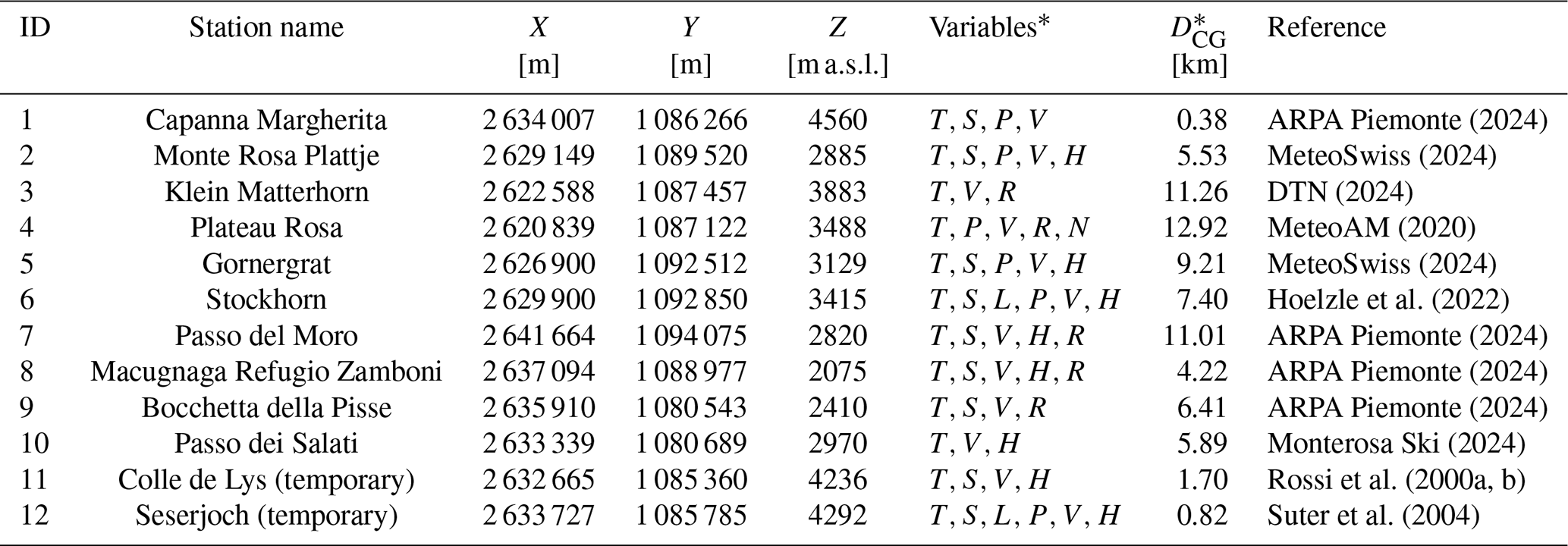
^* Meteorological variable acronyms represent the following. T: air temperature; S: global shortwave radiation; L: longwave radiation; P: atmospheric pressure; V: wind speed; H: relative humidity; R: precipitation; N: cloud cover; D_CG: distance to the saddle point at Colle Gnifetti.

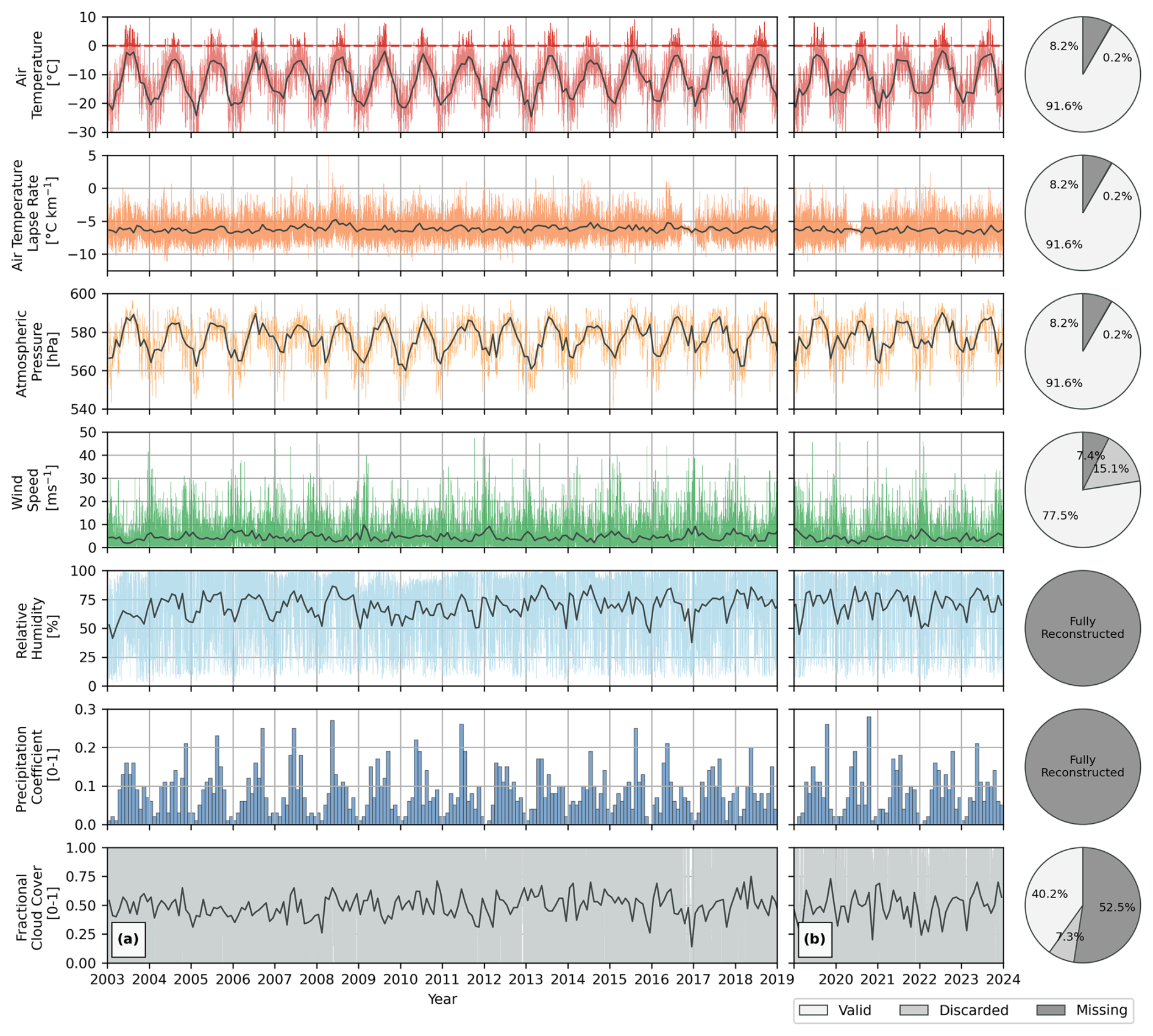
Figure 2 (a) The original quality-checked and gap-filled meteorological time series for the Capanna Margherita produced by Mattea et al. (2021) (2003–2018) and (b) the 5-year extension produced for this study (2019–2023). Hourly values are displayed with monthly means overlain as black lines; monthly cumulative values replace hourly values for the precipitation coefficient. The pie charts show the proportion of meteorological data in our extension directly sourced from CM AWS compared to those requiring reconstruction, due to being discarded during the quality-control processes or missing due to sensor outages.

2 Input data

2.1 Meteorological data

The meteorological forcing for the model is predominantly sourced from the CM AWS, situated on the summit of the Signalkuppe at an altitude of 4560 m a.s.l. Hourly instantaneous values for air temperature, barometric pressure, wind speed and direction, and global radiation are available from mid-2002 to the present day. However, as a result of the extreme operating conditions of the station, sensor malfunctions and outages are of frequent occurrence (Martorina et al., 2003). Mattea et al. (2021) performed a comprehensive quality-control process on the CM series between 2003 and 2018, reconstructing missing data from eight regional high-altitude stations (Fig. 1; ID 4–10 in Table 1) using the technique of quantile mapping (QM) (Cannon et al., 2015; Feigenwinter et al., 2018). We acquired this dataset and then extended the meteorological time series by an additional 5 years up to the end of 2023 by closely replicating the processing steps detailed in Mattea et al. (2021) (Fig. 2). Due to data unavailability, we used the Klein Matterhorn station (ID 3 in Table 1) in lieu of Plateau Rosa for air temperature, relative humidity, and wind speed in our extension of the reconstructed series. However, their respective meteorological time series were found to hold a strong correlation with each other. Two of the required meteorological inputs for the model, relative humidity and fractional cloud cover, are not measured at the CM AWS and are therefore entirely reconstructed. Daytime fractional cloud cover is determined from incoming shortwave radiation measured at the CM AWS, whilst incoming longwave radiation at Stockhorn is used during the night. Relative humidity is estimated as the arithmetic mean of the two highest-altitude stations in the study region: Klein Matterhorn and Stockhorn.

The calibration of several key model parameters is facilitated using meteorological data from high-altitude (>4000 m a.s.l.) temporary weather and energy balance stations in close proximity to CG (Table 3), installed as part of the ALPCLIM project (Auer et al., 2001) (Fig. 1; ID 11–12 in Table 1), specifically the Seserjoch (Suter et al., 2004) and Colle de Lys (Rossi et al., 2000a, b) stations, which were operational from 1998–2000 and 1996–2000 respectively.

2.2 Topographic data

The model spatial grid is derived from a custom-built 20 m resolution digital elevation model (DEM). This was developed by Mattea et al. (2021) by amalgamating the publicly available SwissAlti3D and Piemonte DEMs, neither of which provide full coverage due to the Swiss–Italian border bisecting the study area. The meteorological time series (t) is then projected onto this two-dimensional spatial domain (x, y), creating a three-dimensional model input file (x, y, t). Across the spatial domain, nodal air temperature and pressure are adjusted according to elevation differences using variable lapse rates (derived from the temperature differences between the regional stations (Table 1)) and the barometric equation respectively. The remaining meteorological variables (wind speed, relative humidity, and cloud cover) are assumed constant with elevation.

2.3 Subsurface data

An extensive archive of subsurface data exists at CG that enables model validation. For evaluating the thermal regime, we used a total of 31 temperature profiles extracted from 18 boreholes during the simulation temporal range of 2003–2023. These profiles, detailed in Hoelzle et al. (2011) and GLAMOS (2020, 2022), are mostly concentrated in the vicinity of the saddle point (SP) and on the Signalkuppe flank of CG, but a few are located in the firn facie transition areas around the lower-altitude Seserjoch (Fig. 1a). It is important to note that not all measurements are considered valid; some taken shortly after steam drilling were discarded from our validation set, as some of their thermistor readings were assessed not to be fully equilibrated. Stratigraphic data derived from firn/ice cores obtained at CG (Fig. 1a) (Lier, 2018; Licciulli et al., 2020; Mattea et al., 2021) were also used for the validation of simulated density profiles. Lastly, we installed a continuously logging thermistor chain near the saddle point to measure changes in the firn's thermal regime, from which data are available at a 12 h temporal resolution for 2022.

3 The Coupled Snow and Ice Model in Python

The Coupled Snow and Ice Model in Python (COSIPY), developed by Sauter et al. (2020), combines a skin-layer surface energy balance (SEB) with a one-dimensional multi-layer subsurface model (Cryo Tools, 2022). The original model was unsuccessful at reproducing firn temperatures at CG (Fig. A1 of Appendix A); therefore we had to extensively alter the baseline version 1.4 of COSIPY – often substituting parameterisations for those used in the EBFM (Table 2). This variant, having been developed at the University of Fribourg, will henceforth be referred to as “FRICOSIPY”. This section outlines the model structure, detailing any major modifications we made to the original COSIPY model.

Mattea et al. (2021)Vionnet et al. (2012)Mölg et al. (2009)Wohlfahrt et al. (2016)Mölg et al. (2009)Bougamont et al. (2005)Oerlemans and Knap (1998)Bougamont et al. (2005)Konzelmann et al. (1994)Konzelmann et al. (1994)Konzelmann et al. (1994)Mölg et al. (2012)Sonntag (1994)Sonntag (1994)Essery and Etchevers (2004)Essery and Etchevers (2004)Foken (2008); Stull (1988)Essery and Etchevers (2004)Calonne et al. (2019)Sturm et al. (1997)Yen (1981)Yen (1981)Ligtenberg et al. (2011)Anderson (1976); Boone (2009)Ligtenberg et al. (2011)

Table 2 Parameterisations selected in our FRICOSIPY implementation at CG compared to the default methods used in the baseline version 1.4 of the COSIPY model and the methods used by Mattea et al. (2021) with the energy balance firn model (EBFM).

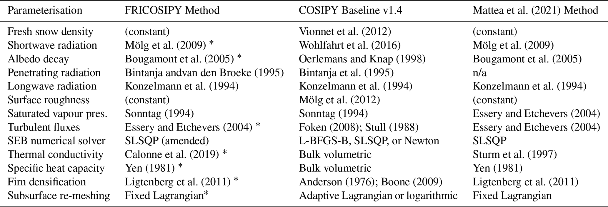
^* New parameterisations added to FRICOSIPY from the baseline version 1.4 of the COSIPY model.

3.1 Surface model

Driven by the meteorological forcing, the surface energy fluxes are evaluated at an infinitesimal skin layer to ascertain the surface temperature (T_s). Based on energy conservation,

$$\begin{array}{}\text{(1)}& {\text{SW}}_{\text{net}}\pm {\text{LW}}_{\text{net}}\pm Q_{\text{sensible}}\pm Q_{\text{latent}}\pm Q_{\text{subsurface}}=Q_{\text{melt}},\end{array}$$

where SW_net is the net shortwave flux, LW_net is the net longwave flux, Q_sensible and Q_latent are the turbulent fluxes for sensible and latent exchange respectively, and Q_subsurface is the subsurface heat conduction flux. The surface temperature is physically constrained to 0 °C; therefore excess energy is apportioned to melt (Q_melt) should this condition arise.

3.1.1 Radiative fluxes

The incident shortwave radiation for a given spatial node (x,y) is modelled after Mölg et al. (2009):

$$\begin{array}{}\text{(2)}& {\text{SW}}_{\text{in}}=\text{TOA}\mathrm{\Lambda }(x,y){\mathit{\tau }}_{\text{rg}}{\mathit{\tau }}_{\text{w}}{\mathit{\tau }}_{\text{a}}{\mathit{\tau }}_{\text{cl}},\end{array}$$

where TOA is the unattenuated top-of-atmosphere radiation and Λ is a correction factor for angle of incidence and topographic shading. The coefficients of atmospheric transmissivity account for Rayleigh scattering and gaseous absorption (τ_rg), water absorption (τ_w), and the attenuation by aerosols (τ_a). These are modelled after Kondratyev (1969), McDonald (1960), and Houghton (1954) respectively. We modified the parameterisation for the attenuation of cloud cover (τ_cl) after Greuell et al. (1997) to maintain parity with the meteorological input of the EBFM:

$$\begin{array}{}\text{(3)}& {\mathit{\tau }}_{\text{cl}}\left(N\right)=\mathrm{1}-aN-b{N}^{\mathrm{2}},\end{array}$$

where a=0.233 and b=0.415 are cloud transmissivity coefficients calibrated to the CM AWS global radiation data and N is the fractional cloud cover. The net shortwave radiation entering the SEB is calculated using a broadband isotropic albedo (α):

$$\begin{array}{}\text{(4)}& {\text{SW}}_{\text{net}}={\text{SW}}_{\text{in}}(\mathrm{1}-\mathit{\alpha })-{\text{SW}}_{\text{pen}},\end{array}$$

where SW_in is the input shortwave radiation and SW_pen represents the penetrating radiation – an apportionment of the shortwave input that bypasses the SEB and directly warms the subsurface layers. This is modelled after Bintanja and van den Broeke (1995), where the absorbed radiation at depth z is calculated as

$$\begin{array}{}\text{(5)}& {\text{SW}}_{\text{pen}}\left(z\right)={\mathit{\lambda }}_{\text{abs}}{\text{SW}}_{\text{in}}(\mathrm{1}-\mathit{\alpha })e^{-z\mathit{\beta }},\end{array}$$

where λ_abs is the fraction of absorbed shortwave radiation (0.8 for ice, 0.9 for snow) and β is the extinction coefficient (2.5 m⁻¹ for ice, 40 m⁻¹ for snow – the latter being adjusted from the default value of 17.1 m⁻¹ to that of a similar study on the Mont Blanc massif by Gilbert et al., 2014).

The evolution of the albedo is modelled after Oerlemans and Knap (1998) as an exponentially decreasing function of time t since the last significant snowfall event (s_min=0.001 m), bounded by prescribed values for fresh snow (α_fresh=0.81) and firn (α_firn=0.52).

$$\begin{array}{}\text{(6)}& \mathit{\alpha }\left(t\right)={\mathit{\alpha }}_{\text{firn}}+\left[({\mathit{\alpha }}_{\text{fresh}}-{\mathit{\alpha }}_{\text{firn}})e^{-\frac{t}{t^{*}}}\right],\end{array}$$

where t^* is the characteristic decay timescale parameter (days). We modified this by adding the enhancement of Bougamont et al. (2005) that enables both a faster decay on a melting surface and slower metamorphism in cold conditions by introducing a dependence on surface temperature (T_s):

$$\begin{array}{}\text{(7)}& t^{*}\left(T_s\right)=\left\{\begin{array}{ll}{t}_{\text{wet}}^{*},& T_{\text{s}}=\mathrm{0}{}^{\circ }\text{C}\\ t_{\text{dry}}^{*}+K\left[\text{max}(T_{\text{s}},T_{\text{max},t^{*}})\right],& T_{\text{s}}<\mathrm{0}{}^{\circ }\text{C},\end{array}\right.\end{array}$$

where $t_{\text{wet}}^{*}$ and $t_{\text{dry}}^{*}$ are the decay timescales (days) for a melting and dry surface respectively, K is a calibration parameter (d °C⁻¹), and $T_{\text{max},t^{*}}$ is a temperature threshold (°C) for the decay timescale adjustment.

Net longwave radiation is calculated in accordance with the Stefan–Boltzmann law for grey body emission:

$$\begin{array}{}\text{(8)}& {\text{LW}}_{\text{net}}={\text{LW}}_{\text{in}}-{\mathit{\epsilon }}_{\text{s}}\mathit{\sigma }{T}_{\text{s}}^{\mathrm{4}},\end{array}$$

where ε_s=0.99 is the glacier surface emissivity and $\mathit{\sigma }=\mathrm{5.67}\times {\mathrm{10}}^{-\mathrm{8}}$ W m⁻² K⁻⁴ is the Stefan–Boltzmann constant. In lieu of any input longwave radiation data at the site, the model parameterises this flux by substituting the air temperature (T_a) and atmospheric emissivity (ε_atm) into the Stefan–Boltzmann law (Konzelmann et al., 1994).

$$\begin{array}{}\text{(9)}& {\displaystyle }& {\displaystyle }{\mathit{\epsilon }}_{\text{atm}}={\mathit{\epsilon }}_{\text{cs}}(\mathrm{1}-N^{\mathrm{2}})+{\mathit{\epsilon }}_{\text{clouds}}{N}^{\mathrm{2}},\text{(10)}& {\displaystyle }& {\displaystyle }{\mathit{\epsilon }}_{\text{cs}}=\mathrm{0.23}+c_{\text{emission}}{\left({\displaystyle \frac{v{p}_{\text{sat}}\mathrm{RH}}{T_{\text{a}}}},\right)}^{\mathrm{0.125}}\end{array}$$

where vp_sat is the saturated vapour pressure (Pa) determined as a function of temperature using the parameterisation of Sonntag (1994), RH is the relative humidity (%), ε_cs and ε_clouds=0.96 are the clear-sky and cloud emissivities respectively, and c_emission=0.42 is a calibration parameter.

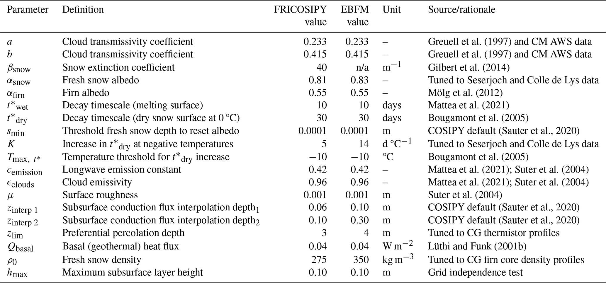
Greuell et al. (1997)Greuell et al. (1997)Gilbert et al. (2014)Mölg et al. (2012)Mattea et al. (2021)Bougamont et al. (2005)(Sauter et al., 2020)Bougamont et al. (2005)Mattea et al. (2021); Suter et al. (2004)Mattea et al. (2021); Suter et al. (2004)Suter et al. (2004)(Sauter et al., 2020)(Sauter et al., 2020)Lüthi and Funk (2001b)

Table 3 Model parameter values selected in our FRICOSIPY implementation at CG compared to those used by Mattea et al. (2021) with the energy balance firn model (EBFM) of van Pelt et al. (2012). A brief explanation or reference for parameter selection is also provided. Further information on the implications of adjusting these parameters is provided in the model sensitivity study (Appendix B).

3.1.2 Turbulent fluxes

The turbulent fluxes are calculated according to a bulk aerodynamic approach after Foken (2008) and Stull (1988):

$$\begin{array}{}\text{(11)}& {\displaystyle }& {\displaystyle }{Q}_{\text{sensible}}={\mathit{\rho }}_{\text{a}}{c}_{\text{p,a}}{C}_{\text{h}}{V}_{\text{a}}(T_{\text{a}}-T_{\text{s}}),\text{(12)}& {\displaystyle }& {\displaystyle }{Q}_{\text{latent}}={\mathit{\rho }}_{\text{a}}{L}_{\text{s,v}}{C}_{\text{h}}{V}_{\text{a}}(q_{\text{a}}-q_{\text{s}}),\end{array}$$

where ρ_a is the dry air density (kg m⁻³), c_p,a is the specific heat of dry air under constant pressure (J kg⁻¹ K⁻¹), V is the wind speed (m s⁻¹), L_s,v is the latent heat of sublimation or vaporisation (J kg⁻¹), q is the specific humidity (kg kg⁻¹), and the s and a subscripts refer to the surface and the atmosphere at a measurement height of 2 m respectively. We adapted the calculation of the turbulent exchange coefficient C_h to follow the approach of Essery and Etchevers (2004):

$$\begin{array}{}\text{(13)}& {\displaystyle }& {\displaystyle }{C}_{\text{h}}=C_{\text{hn}}{\mathrm{\Psi }}_{\mathit{Ri}},\text{(14)}& {\displaystyle }& {\displaystyle }{C}_{\text{hn}}={\mathit{\kappa }}^{\mathrm{2}}{\left[\text{log}\left({\displaystyle \frac{z_{\text{a}}}{\mathit{\mu }}}\right)\right]}^{-\mathrm{2}},\end{array}$$

where C_hn is the value under neutral conditions, κ is the von Karman constant (0.40), and μ is the surface roughness (m). The stability function (Ψ_Ri), derived from the bulk Richardson number (Ri_b), represents a correction for the stability of the atmospheric boundary layer.

$$\begin{array}{}\text{(15)}& {\displaystyle }& {\displaystyle }{\mathrm{\Psi }}_{\mathit{Ri}}=\left\{\begin{array}{ll}(\mathrm{1}+\mathrm{10}{\mathit{Ri}}_{\text{b}}{)}^{-\mathrm{1}},& R{i}_{\text{b}}\ge \mathrm{0}\\ (\mathrm{1}-\mathrm{10}{\mathit{Ri}}_{\text{b}}{\left(\mathrm{1}+\mathrm{10}{C}_{\text{hn}}\frac{\sqrt{-{\mathit{Ri}}_{\text{b}}}}{f_z}\right)}^{-\mathrm{1}},& {\mathit{Ri}}_{\text{b}}<\mathrm{0};\end{array}\right.\text{(16)}& {\displaystyle }& {\displaystyle }R{i}_{\text{b}}={\displaystyle \frac{g{z}_{\text{a}}}{V_{\text{a}}^{\mathrm{2}}}}\left[{\displaystyle \frac{T_{\text{a}}-T_{\text{s}}}{T_{\text{a}}}}+{\displaystyle \frac{q_{\text{a}}-q_s}{q_{\text{a}}+\mathit{ϵ}(\mathrm{1}-\mathit{ϵ})}}\right];\text{(17)}& {\displaystyle }& {\displaystyle }{f}_z={\displaystyle \frac{\mathrm{1}}{\mathrm{4}}}\sqrt{{\displaystyle \frac{\mathit{\mu }}{z_{\text{a}}}}};\end{array}$$

where g is the gravitational acceleration (m s⁻²) and ϵ is the ratio of molecular weights between water and dry air. By default, surface roughness (μ) evolution in the COSIPY model is modelled after Mölg et al. (2012) as a linearly increasing function of time t since the last snowfall event. However, we considered this unrepresentative of the snow surface conditions at CG that are more heavily influenced by scouring during extreme wind events. Therefore, we use a constant value of 0.001 m derived by Suter et al. (2004) from wind profile measurements at Seserjoch.

3.1.3 Subsurface conduction flux

The subsurface heat conduction flux is determined based on the near-surface temperature gradient:

$$\begin{array}{}\text{(18)}& Q_{\text{subsurface}}=k_{\text{s}}\left[{\displaystyle \frac{T_{z\text{interp\hspace{0.25em}2}}-T_{z\text{interp\hspace{0.25em}1}}}{z_{\text{interp\hspace{0.25em}2}}-z_{\text{interp\hspace{0.25em}1}}}}\right],\end{array}$$

where k is the thermal conductivity (W m⁻¹ K⁻¹) and z_interp 1 = 0.06 m and z_interp 2 = 0.10 m are prescribed depth values used to calculate subsurface temperatures via linear interpolation between subsurface layers.

3.1.4 Precipitation model

In order to represent the extreme spatial gradient of snow accumulation at the site, we replace the spatially homogeneous precipitation input with a three-phase anomaly method that was previously employed to the site by Mattea et al. (2021). As the dimensionality of the model cannot represent lateral mass transportation, this technique artificially adjusts nodal precipitation to accommodate for preferential deposition and losses from wind scouring to enable a representative accumulation rate. This is achieved by temporally downscaling a spatially variable annual accumulation climatology into an hourly precipitation time series with adjustments for annual variability – the assumption being that, in a cold infiltration zone, any mass ablation though melt is internally retained within the firn. However, this leaves mass losses from sublimation unaccounted for, leading to a considerable under-representation of accumulation – up to 31 % on the SK. Therefore, we enhance the original method of Mattea et al. (2021) with an annually variable correction for sublimation losses, such that, for a given grid cell (x, y) at simulation time step t in year i, nodal precipitation (R) is determined as

$$\begin{array}{}\text{(19)}& R(x,y,t)=\left[C(x,y)A_{\text{acc}}\left(i\right)+S(x,y)A_{\text{sub}}\left(i\right)\right]D\left(t\right),\end{array}$$

where C is the long-term annual accumulation climatology (m w.e. yr⁻¹), S is the pre-modelled mean annual sublimation climatology (m w.e. yr⁻¹), A_acc and A_sub are the annual anomalies for accumulation and sublimation respectively, and D is the temporal downscaling coefficient. The exact formulation of the original accumulation climatology raster (Fig. 3) – derived from GPR profiles (Konrad et al., 2013), snow stakes (Suter and Hoelzle, 2002), and firn cores (Lier, 2018; Licciulli et al., 2020) – and the annual accumulation anomaly is explained in greater detail in Mattea et al. (2021).

As hourly precipitation data are not measured at the AWS CM, the downscaling coefficient (D) is calculated by normalising to a unit sum the average hourly precipitation rates from the closest rain gauges at Passo del Moro, Bochetta della Pisse, and Rifugio Macugnaga Zamboni (Fig. 1; ID 7–9 in Table 1). The model then uses a linear logistic transfer function based on air temperature to differentiate between solid and liquid precipitation. The proportion of snowfall therefore scales between 100 % at 0 °C and 0 % at 2 °C (Hantel et al., 2000). In COSIPY, the density of newly added fresh snow layers (ρ₀) is determined as a function of air temperature and wind speed after Vionnet et al. (2012). However we reverted to using a constant value of 275 kg m⁻³, given the incompatibility and complications of using this approach coupled with our artificial precipitation model.

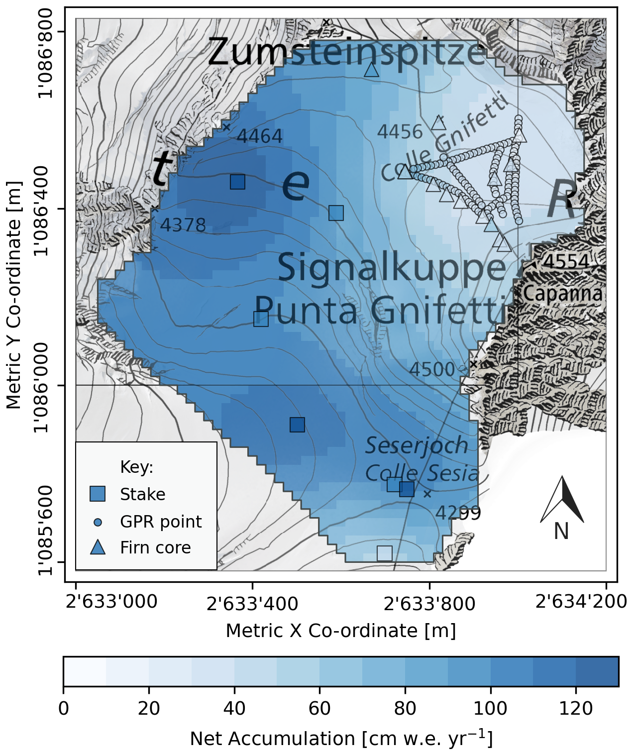
Figure 3 Annual accumulation climatology forming the spatial component of the precipitation model (Mattea et al., 2021). Spatial co-ordinates are defined by EPSG 2056 (Metric Swiss CH1903+/LV95). Topographic map source: Swisstopo (2017).

3.2 Subsurface model

Subsurface layers are discretised according to an adaptive Lagrangian re-meshing algorithm within COSIPY: layers can translate vertically in the grid following mass exchange at the surface and are merged with adjacent layers if user-defined temperature or density thresholds are exceeded. We found subsurface layer properties to be particularly sensitive to the selection of the re-meshing algorithm, with the adaptive method imparting a large positive density bias against observed firn core profiles (Appendix A). Therefore, we adopted an alternative approach: instead of creating new subsurface layers on every precipitation event as with the adaptive algorithm, the new approach instead collates new accumulation into the uppermost layer until a fixed height threshold (h_max) is reached and prohibits any layer-merging.

3.2.1 Thermal diffusion

The evolution of the subsurface thermal regime is driven by the processes of thermal diffusion, water refreezing, and subsurface melting:

$$\begin{array}{}\text{(20)}& \mathit{\rho }{c}_{\text{p}}{\displaystyle \frac{\mathit{\delta }T}{\mathit{\delta }t}}={\displaystyle \frac{\mathit{\delta }}{dz}}\left(k{\displaystyle \frac{\mathit{\delta }T}{dz}}\right)+L_{\text{m}}\left(F-M\right),\end{array}$$

where ρ, c_p, and k are the effective density (kg m⁻³), specific heat capacity (J kg⁻¹ K⁻¹), and thermal conductivity (W m⁻¹ K⁻¹) of subsurface firn layers; L_m is the latent heat of melting (J kg⁻¹); and F and M are the refreezing and subsurface melting rates (kg m⁻³ s⁻¹) respectively. By default, COSIPY resolves Eq. (20) with a fixed temperature at the base of the modelling domain; however, we substituted this for a basal (geothermal) heat flux (Q_basal).

The model defines subsurface layers according to their volumetric fraction of ice (ϕ_ice), water (ϕ_water), and air (ϕ_air) (Eq. 21), with their inherent physical properties (such as their thermal conductivity (k)) derived as a weighted sum of their fractional composition (Eq. 22).

$$\begin{array}{}\text{(21)}& {\displaystyle }& {\displaystyle }{\mathit{\varphi }}_{\text{ice}}+{\mathit{\varphi }}_{\text{water}}+{\mathit{\varphi }}_{\text{air}}=\mathrm{1}\text{(22)}& {\displaystyle }& {\displaystyle }k=k_{\text{ice}}{\mathit{\varphi }}_{\text{ice}}+k_{\text{water}}{\mathit{\varphi }}_{\text{water}}+k_{\text{air}}{\mathit{\varphi }}_{\text{air}}\end{array}$$

However, this basic approach significantly overestimates thermal conductivity at low densities (Calonne et al., 2019), leading to an inability for the firn to retain thermal energy. Therefore we substituted the default bulk volumetric method (Eq. 22) with the empirical formulation of Calonne et al. (2019) that instead defines thermal conductivity as

$$\begin{array}{ll}{\displaystyle }& {\displaystyle }k(\mathit{\rho },T)=(\mathrm{1}-\mathit{\vartheta }){\displaystyle \frac{k_i\left(T\right)k_{\text{a}}\left(T\right)}{k_i^{\text{ref}}{k}_{\text{a}}^{\text{ref}}}}{k}_{\text{snow}}^{\text{ref}}\left(\mathit{\rho }\right)\\ \text{(23)}& {\displaystyle }& {\displaystyle }+\mathit{\vartheta }{\displaystyle \frac{k_i\left(T\right)}{k_i^{\text{ref}}}}{k}_{\text{firn}}^{\text{ref}}\left(\mathit{\rho }\right),\text{(24)}& {\displaystyle }& {\displaystyle }\mathit{\vartheta }=\mathrm{1}/\left[\mathrm{1}+\text{exp}(-\mathrm{2}a(\mathit{\rho }-{\mathit{\rho }}_{\text{transition}}\left)\right)\right],\text{(25)}& {\displaystyle }& {\displaystyle }{k}_{\text{firn}}^{\text{ref}}=\mathrm{2.107}+\mathrm{0.003618}(\mathit{\rho }-{\mathit{\rho }}_i),\text{(26)}& {\displaystyle }& {\displaystyle }{k}_{\text{snow}}^{\text{ref}}=\mathrm{0.024}-\mathrm{1.23}\mathit{\rho }\times {\mathrm{10}}^{-\mathrm{4}}+\mathrm{2.5}\times {\mathrm{10}}^{-\mathrm{6}}{\mathit{\rho }}^{\mathrm{2}},\end{array}$$

where k_i(T) and k_a(T) are the ice and air thermal conductivity at the temperature T, $k_i^{\text{ref}}=\mathrm{2.107}$ W m⁻¹ K⁻¹ and $k_{\text{a}}^{\text{ref}}=\mathrm{0.024}$ W m⁻¹ K⁻¹ are the ice and air thermal conductivities at the reference temperature of −3 °C, a=0.02 m³ kg⁻¹, and ρ_transition=450 kg m⁻³.

We also switched to using the empirical temperature-dependent specific heat capacity of Yen (1981), as opposed to the default bulk volumetric approach:

$$\begin{array}{}\text{(27)}& c_{\text{p}}\left(T\right)=\mathrm{152.2}+\mathrm{7.122}T.\end{array}$$

3.2.2 Percolation scheme

COSIPY employs a standard “bucket approach” percolation scheme whereby liquid water filters down into subsequent layers upon exceeding the layer saturation capacity. We supplemented this with the statistical deep preferential percolation scheme of Marchenko et al. (2017) (as used in the EBFM), which initially instantly distributes all surface water in accordance with a normal probability density function (PDF) up to a pre-defined characteristic preferential percolation depth (z_lim):

$$\begin{array}{}\text{(28)}& {\displaystyle }& {\displaystyle }{\text{PDF}}_{\text{normal}}(z,z_{\text{lim}})=\mathrm{2}\left[{\displaystyle \frac{\text{exp}\left(-\frac{z^{\mathrm{2}}}{\mathrm{2}{\mathit{\sigma }}^{\mathrm{2}}}\right)}{\mathit{\sigma }\sqrt{\mathrm{2}\mathit{\pi }}}}\right],\text{(29)}& {\displaystyle }& {\displaystyle }\mathit{\sigma }=z_{\text{lim}}/\mathrm{3},\end{array}$$

where σ is the standard deviation of the probability density function and z_lim represents the pre-defined characteristic preferential percolation depth (m). We tuned this value to 3 m to match 20 m depth firn temperatures at CG.

Penetrating shortwave radiation (see Sect. 3.1.1) can also directly melt the ice matrix of subsurface layers if they are warmed to the melting temperature, supplementing their water content. Subsurface water can subsequently refreeze if there is sufficient cold content and volumetric capacity in layers – the latter being limited by the pore closure density of 830 kg m⁻³ at the transition from firn to glacial ice. Any remaining water is stored by capillary and adhesive forces (irreducible water content), with the excess being drained into deeper layers via the original bucket scheme. The maximum irreducible water (θ_irr) is based on the volumetric ice fraction of subsurface layers (Coléou and Lesaffre, 1998; Wever et al., 2014).

$${\mathit{\theta }}_{\text{irr}}=\left\{\begin{array}{ll}\mathrm{9.0264}+\mathrm{0.0099}\frac{(\mathrm{1}-{\mathit{\varphi }}_{\text{ice}})}{{\mathit{\varphi }}_{\text{ice}}},& {\mathit{\varphi }}_{\text{ice}}\le \mathrm{0.23}\\ \mathrm{0.08}-\mathrm{0.1023}({\mathit{\varphi }}_{\text{ice}}-\mathrm{0.03}),& \mathrm{0.23}>{\mathit{\varphi }}_{\text{ice}}\le \mathrm{0.812}\\ \mathrm{0},& {\mathit{\varphi }}_{\text{ice}}>\mathrm{0.812}\end{array}\right.$$

Water reaching the base of the computational domain is instantly removed and recorded as runoff.

3.2.3 Firn densification

By default, dry firn densification is modelled in COSIPY after Boone (2009), accounting for compaction from overburden pressure and the thermal metamorphosis of snow. As a result of difficulties encountered using this method to generate firn density profiles representative of those observed at CG, we switched to the semi-empirical method of Arthern et al. (2010) based on the processes of sintering and lattice-diffusion creep of consolidated ice. An enhancement by Ligtenberg et al. (2011) furthers this by adding a dependence on the local accumulation rate:

$$\begin{array}{ll}\text{(30)}& {\displaystyle }& {\displaystyle \frac{\mathrm{d}\mathit{\rho }}{\mathrm{d}t}}=C{c}_{\text{lig}}g(\mathit{\rho }-{\mathit{\rho }}_{\text{ice}})\text{exp}\left(-{\displaystyle \frac{E_{\text{c}}}{RT}}+{\displaystyle \frac{E_{\text{g}}}{R\stackrel{\mathrm{‾}}{T}}}\right);{\displaystyle }& {\displaystyle }{c}_{\text{lig}}(C,\mathit{\rho })\\ \text{(31)}& {\displaystyle }& {\displaystyle }=\left\{\begin{array}{ll}\mathrm{0.0991}-\mathrm{0.0103}\text{log}\left(C\right),& \mathit{\rho }<\mathrm{550}{\text{kg\hspace{0.25em}m}}^{-\mathrm{3}}\\ \mathrm{0.0701}-\mathrm{0.0086}\text{log}\left(C\right),& \mathit{\rho }\ge \mathrm{550}{\text{kg\hspace{0.25em}m}}^{-\mathrm{3}};\end{array}\right.\end{array}$$

where C is the accumulation rate (mm yr⁻¹), ρ is the layer density (kg m⁻³), T is the current layer temperature (°C), $\stackrel{\mathrm{‾}}{T}$ is the average layer temperature of the preceding year (°C), R=8.314 J mol⁻¹ K⁻¹ is the universal gas constant, and E_c=60 kJ mol⁻¹ and E_g = 42.4 kJ mol⁻¹ are the activation energies associated with creep by lattice diffusion and grain growth respectively. The processes of meltwater refreezing and subsurface melting also change the fractional constituents of subsurface layers, thereby altering their density into addition to the process of dry firn densification.

3.3 Model initialisation

In order to initialise the model subsurface to steady-state conditions, the main simulation was preceded by a 64-year spin-up using a reconstructed 1939–2002 meteorological forcing. The historic mean monthly air temperature (MMAT) at CM during this period was estimated using quantile mapping of the long-term air temperature series from Jungfraujoch (3454 m a.s.l.) (MeteoSwiss, 2024), which holds a strong Pearson's correlation of 0.97 when comparing the stations' data from the establishment of the CM AWS in 2002 to the present day. Representative months were then selected from the existing 2003–2023 meteorological time series based on this MMAT, with any remaining bias subsequently removed. This ensures that the model spin-up air temperature, the principal meteorological variable controlling surface melt and the subsurface thermal regime, is accurate, thus enabling firn temperatures to initialise to values representative of the start of the 21st century.

The simulation depth was set to a limit of 50 m, using subsurface layers up to a maximum height of 10 cm. Beyond a threshold depth of 21 m, coarser 1 m height layers are used for greater computational efficiency, giving an average of 500 layers per node due to layer compaction. After initialisation, the main simulation runs with an hourly temporal and 20 m spatial resolution for a 21-year period between 2003 and 2023.

4 Results

While FRICOSIPY outputs a large selection of surface and subsurface variables, in this section we predominantly focus on those that influence the thermal regime of a cold firn facie. Starting with the simulated surface energy exchanges and the resultant quantities of sublimation and surface melt, we proceed to report on the energy release from deep meltwater percolation and the subsequent diffusion of heat to depth that leads to sustained firn warming.

4.1 Surface energy and mass exchanges

There is strong spatial variability in modelled surface exchanges across CG (Fig. 4), driven by the topographically derived insolation gradient. The exposed south-facing aspect of the Zumsteinspitze slope (ZS) receives the greatest shortwave flux and correspondingly expends a greater amount of energy through surface melt compared to the Signalkuppe slope (SK). However, melt is mostly limited to the summer months at CG, and, even in July, the melt flux does not exceed 6 % of the monthly energy turnover at the saddle point (SP). Turbulent exchange also makes a significant contribution to monthly energy turnover at CG, although it has a high temporal variability due to its the dependence on the wind speed in the model parameterisation (Eqs. 11–12). During winter at the SK, sensible heat is an even greater energy source than shortwave radiation due to the steep temperature gradient modelled between the surface and the air. Sensible exchange is conversely less influential at the ZS in winter, as the surface temperature is higher due to greater insolation. The prevalence of cold, dry air in the meteorological forcing means the endothermic process of sublimation represents 87 % of turbulent mass exchange. Deposition, by contrast, accounts for the remaining 13 % and typically requires the relative humidity to exceed 90 % to reverse the prevailing moisture gradient. Therefore, net latent exchange acts predominantly as an energy sink and plays a vital role in inhibiting surface melt, given that the magnitude of longwave emission is physically limited by the surface temperature constraints. Indeed, the simulation of surface melt occurs almost exclusively at wind speeds below 5 m s⁻¹, when latent exchange is limited. However, despite the much greater dissipation of energy via latent exchange, annual surface mass ablation via sublimation averages 12.2 cm w.e. yr⁻¹ at CG and rarely exceeds melt as a result of the latent heat of sublimation (2.83 × 10⁶ J kg⁻¹) being 1 order of magnitude greater than melting (3.34 × 10⁵ J kg⁻¹).

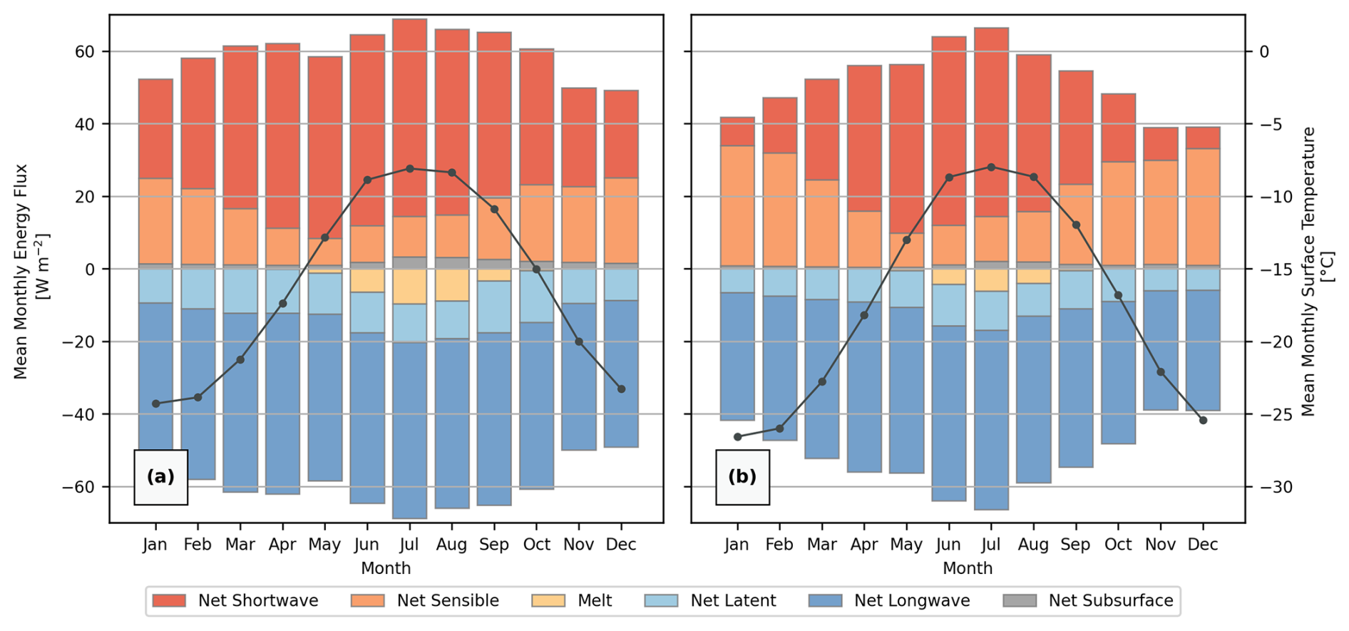
Figure 4 Modelled mean monthly surface energy fluxes (2003–2023) at (a) the Zumsteinspitze slope (ZS) and at (b) the Signalkuppe slope (SK) with mean monthly surface temperature overlain on the secondary y axis (20 m spatial and 1 h temporal resolution). The SEB of the saddle point (SP) is not displayed but possesses approximately intermediary values between the displayed locations.

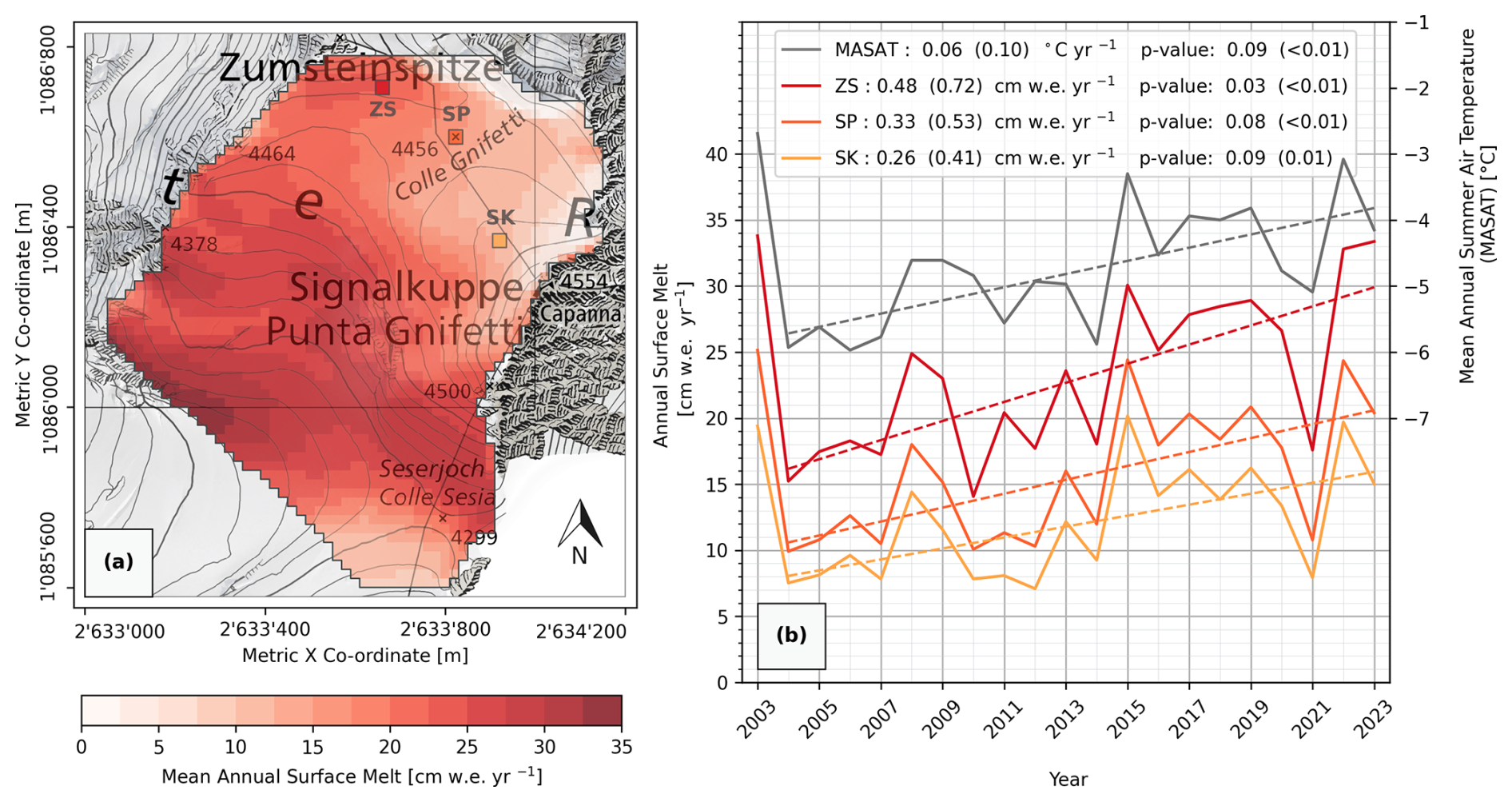
Figure 5 (a) Modelled mean annual surface melt (2003–2023). (b) Modelled annual surface melt (2003–2023) at the three CG reference locations (solid lines; Zumsteinspitze slope (ZS), saddle point (SP), Signalkuppe slope (SK)) compared to mean annual summer air temperature (MASAT). Linear regression trends, calculated excluding the extreme-melt year of 2003, are displayed as dashed lines. Annual trends are reported for the full 2003–2023 simulation period (first number) and excluding the extreme-melt year of 2003 (second number, in parentheses). Spatial co-ordinates are defined by EPSG 2056 (Metric Swiss CH1903+/LV95). Topographic map and orthoimage sources: Swisstopo (2017, 2023).

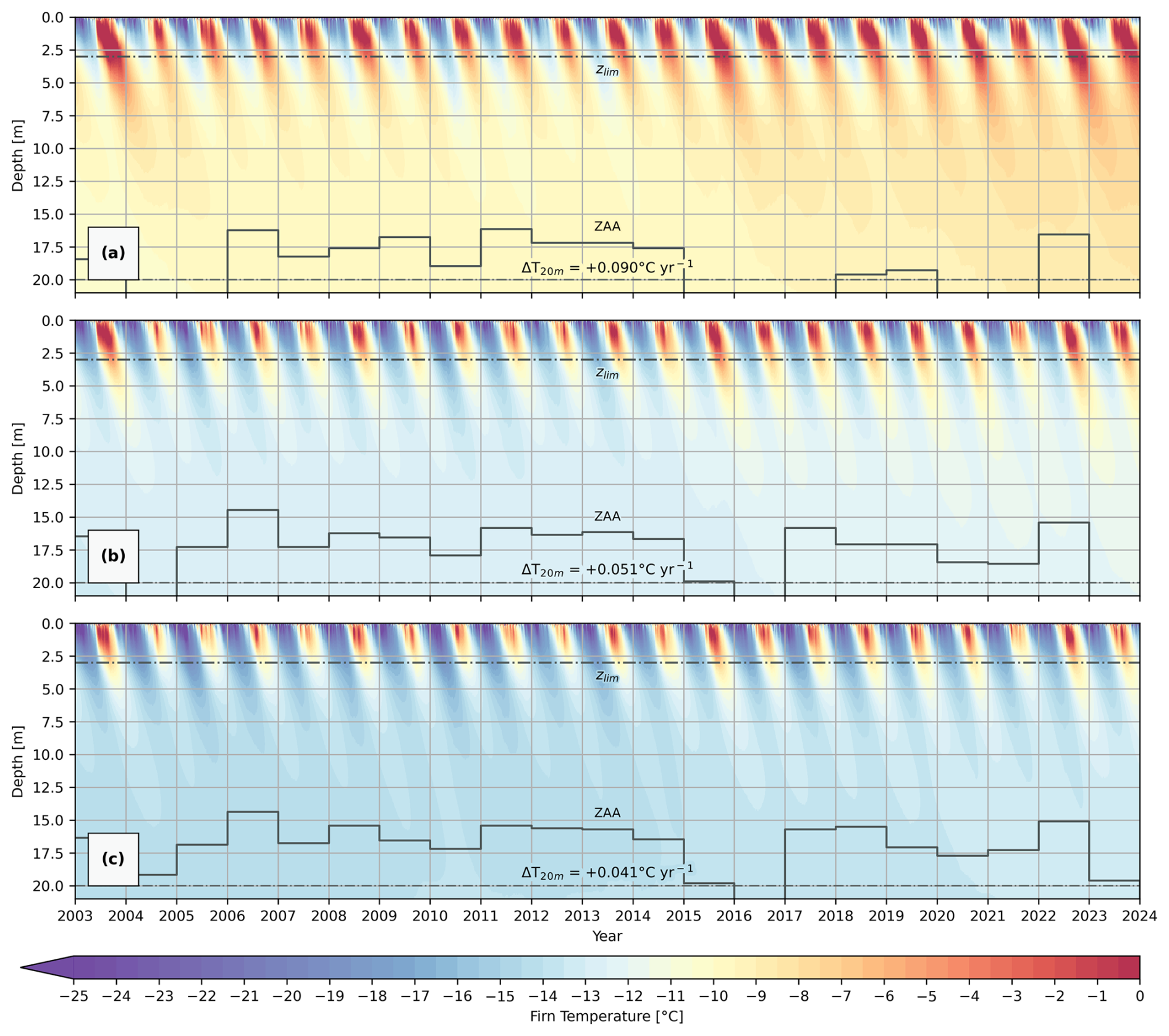
Figure 6 Modelled firn temperature–depth profiles at the (a) Zumsteinspitze slope (ZS), (b) saddle point (SP), and (c) Signalkuppe slope (SK) (2003–2023) (20 m spatial and 1 h temporal resolution). Zero annual amplitude (ZAA) (ΔT<0.1 °C) depth is overlain as a line graph. Firn warming rates over the 21-year simulation at 20 m depth (ΔT_20 m) are also indicated in the figure.

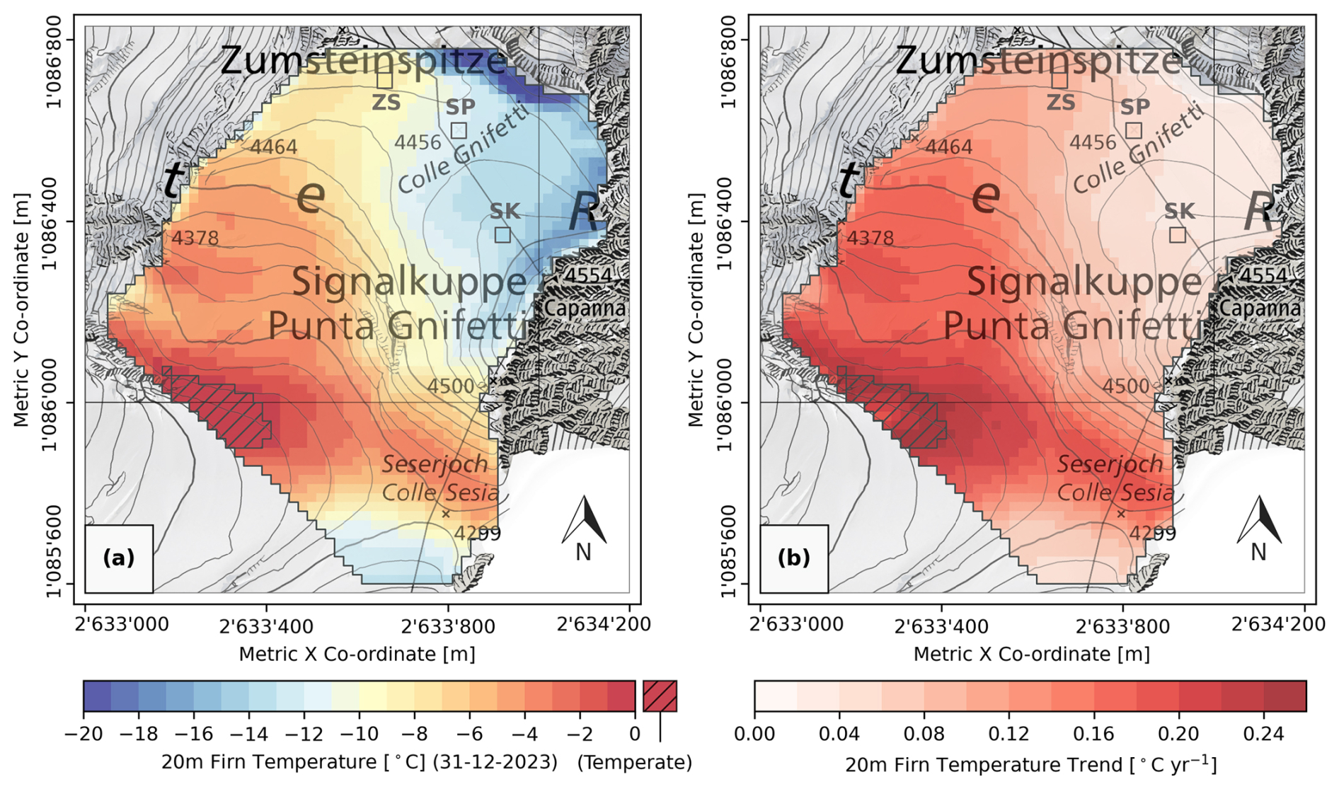
Figure 7 (a) Modelled 20 m depth firn temperatures on the simulation end date of 31 December 2023 and (b) the 20 m depth firn evolution during the full 21-year simulation range (2003–2023) (20 m spatial and 1 h temporal resolution). Spatial co-ordinates are defined by EPSG 2056 (Metric Swiss CH1903+/LV95). Topographic map and orthoimage sources: Swisstopo (2017, 2023). Initial firn temperatures are shown in Fig. S1 of the Supplement.

4.2 Melt

The spatial distribution of modelled mean annual surface melt (Fig. 5a) largely corresponds with the patterns of modelled surface exchanges, with variation strongly influenced by differences in nodal elevation, aspect, and slope. Across the reference locations at CG, it ranges between 12.4 cm w.e. yr⁻¹ at the SK, 16.1 cm w.e. yr⁻¹ at the SP, and 23.5 cm w.e. yr⁻¹ at the ZS, with the lower-altitude slopes of the Grenzgletscher reaching a maximum of 34.8 cm w.e. yr⁻¹. Conversely, some of the north-facing margins of the Signalkuppe have negligible to no modelled surface melt, indicative of the re-crystallisation firn facie zone. Despite strong inter-annual fluctuations, statistically significant trends in increasing annual surface melt can be identified at CG – particularly if the extreme-melt year of 2003, driven by an unprecedented European summer heatwave (Schär et al., 2004), is not considered (Fig. 5b). Linear least-squares regression from 2004–2023 yields an increase in surface melt ranging from 0.41 cm w.e. yr⁻² at the SK, 0.53 cm w.e. yr⁻² at the SP, and 0.72 cm w.e. yr⁻² at the ZS. Annual variation in modelled melt holds a strong Pearson's correlation of 0.90 to the mean annual summer air temperature (MASAT) recorded at the CM AWS, which increases by 0.10 °C yr⁻¹ over this time period.

Modelled subsurface melt generally adheres to the same spatiotemporal patterns of surface melt but accounts for an average of only 15.8 % of combined surface and subsurface melt at the SP. The process is mostly confined to the uppermost metre of the firn, with 82.3 % of simulated subsurface melt events happening on time steps with surface melt occurring simultaneously. The remainder predominantly occur following surface melt events in clear-sky conditions, when abrupt increases in wind speed suppress simulated melt at the surface. Notably, the simulation of surface melt is not restricted to time steps with positive air temperatures; 19.4 % of the total melt recorded at the SP occurs during sub-zero air temperatures.

4.3 Firn temperatures

Whilst simulated near-surface firn temperatures are subject to a high degree of inter-annual fluctuation due to their strong coupling to the applied meteorological forcing, progressively deeper layers become more thermally isolated (Fig. 6). Simulated meltwater refreezing events can be visually identified in Fig. 6 by steep protrusions of near-zero degree temperatures into the depths of the firn following summer melt events – particularly evident at the ZS in Fig. 6a in high-melt years such as 2003, 2015, and 2022. In contrast, the magnitude of these events is considerably smaller at the SP and SK, resulting in reduced firn warming. The depth of meltwater refreezing events is constrained in the simulation by the percolation parameterisation of Marchenko et al. (2017) and the characteristic depth z_lim set to 3 m, but exceedance of this limit is possible if all overlying layers become saturated. Nevertheless, this rarely occurs at these reference locations, and 85.2 % of simulated refreezing occurs above a depth of 3 m at CG. Thermal diffusion and vertical advection subsequently transport thermal energy to the full depth of the simulated domain following a lag period of approximately 2 years. At a depth of 20 m, modelled annual firn temperature variation rarely exceeds ±0.1 °C, except following extreme-melt years such as 2003, 2015, and 2022, and is therefore considered indicative of long-term climatic changes.

Corresponding with the spatial patterns of surface melt, there are similarly strong gradients in the modelled 20 m depth firn temperature that generally reflect changes in elevation and surface aspect (Fig. 7a). At CG, temperatures range between −13.35 °C at the SK and −8.51 °C at the ZS over a lateral distance of less than 500 m, a temperature gradient of 1.13 °C 100 m⁻¹. On the lower-altitude south-facing slopes of the Grenzgletscher, towards the southwestern region of the spatial domain, modelled deep-firn temperatures reach those of a temperate firn facie by the summer of 2022, coinciding with the area of greatest simulated surface melt (Fig. 5a).

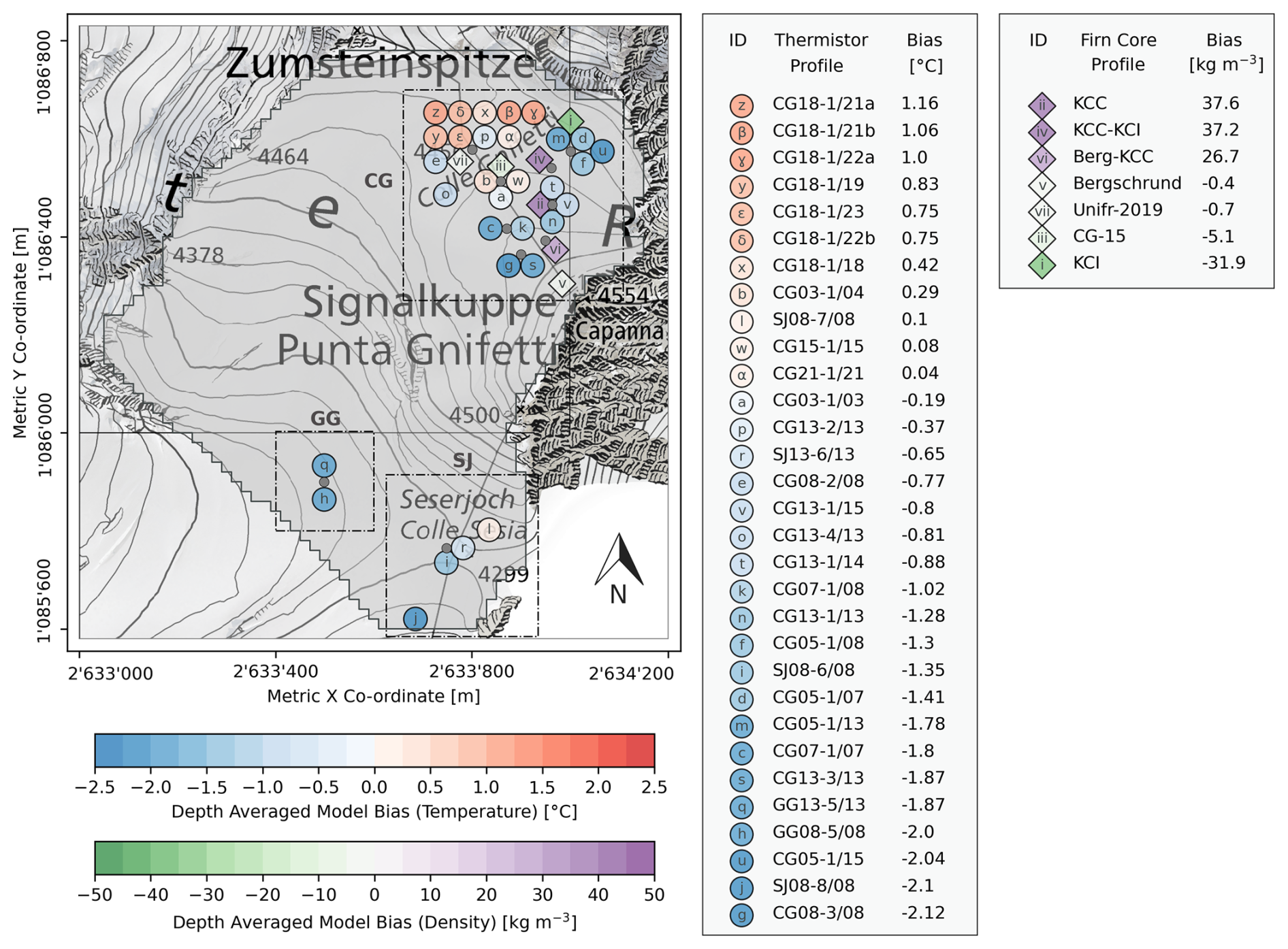
Figure 8 Depth-averaged model temperature and density bias across the computational domain. Borehole thermistor profile codes have the designation LLYY-I/yy, where “LL” indicates the borehole location (either Colle Gnifetti (CG), Seserjoch (SJ), or Grenzgletscher (GG)), “YY-I” gives the drilling year and index number of the borehole, and “yy” specifies the year the temperature profile was measured (Hoelzle et al., 2011; GLAMOS, 2020, 2022, 2024). Spatial co-ordinates are defined by EPSG 2056 (Metric Swiss CH1903+/LV95). Topographic map and orthoimage sources: Swisstopo (2017, 2023). Individual profile comparisons are provided in Figs. S3, S4, and S5 of the Supplement.

Simulated firn warming at the SP is 0.051 °C yr⁻¹, equating to a 1.07 °C increase over the course of the 21-year simulation. There is considerable variation across the saddle consistent with the previously displayed spatial patterns of melt and temperature; however, these changes are modest compared to the lower-elevation regions (Fig. 7b). In these areas at the southwestern reaches of the domain, englacial warming rates are much greater up to a maximum of 0.27 °C yr⁻¹, almost 4 times the local recorded rate of atmospheric warming of 0.073 °C yr⁻¹ from the CM AWS time series, calculated using linear least-squares regression of mean annual air temperature (MAAT) (p value < 0.01). The irregularities in the warming rates in this area are as a result of some locations reaching temperate conditions (hatched area in Fig. 7a and b), where further warming is physically constrained as it attains the melting point.

4.4 Model validation

Depth-averaged model firn temperature bias ranges between −2.12 and 1.16 °C, when compared to borehole thermistor measurements (Fig. 8). This corresponds to an average of −0.65 °C or a root-mean-square error (RMSE) of 1.28 °C. Spatially, model residuals show a tendency to significantly underestimate firn temperatures around the periphery of the Signalkuppe flank at CG and at lower elevations at the Seserjoch (SJ) and Grenzgletscher (GG). In the case of the latter two locations, the model initialises firn temperatures several degrees lower than historic measurements from 1999 (Suter and Hoelzle, 2002), preceding the simulation temporal range, which is counterbalanced by an excessive warming rate (Fig. 7b). Simulated density profiles on average have a slight positive density bias of 9.0 kg m⁻³ and RMSE of 70.6 kg m⁻³; however, firn core profiles are spatially limited to a small extent of the modelling domain around CG.

4.5 Englacial warming at Colle Gnifetti

The simulation results can also be assessed temporally against historic englacial temperature measurements from CG. Since 1991, measured 20 m depth temperatures at the SP have increased by 1.52 °C at a rate of 0.046 °C yr⁻¹ over the 33-year period (Figs. 9 and 10); the previous decade between 1982 and 1991 had a change of less than 0.1 °C. Notably, the rate of observed firn warming is considerably slower than the 21-year trend in mean annual air temperature (MAAT) at the CM AWS from 2003 of 0.073 °C yr⁻¹ (p value < 0.01). However, the QM reconstruction of the air temperature series for CM using data from Jungfraujoch (3454 m a.s.l.) indicates there is no evidence of a significant trend from 1991–2002.

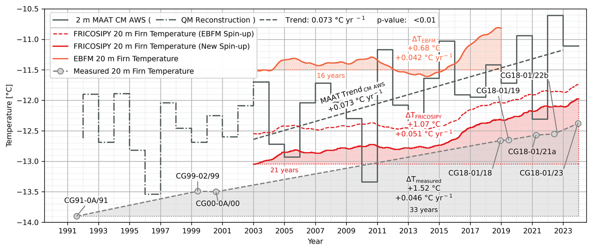
Figure 9 Measured englacial warming at the CG SP compared to the FRICOSIPY simulation (Haeberli and Funk, 1991; Suter et al., 2001; Suter and Hoelzle, 2002; GLAMOS, 2020, 2022, 2024), previous modelling efforts using the EBFM of van Pelt et al. (2012) (Mattea et al., 2021), and the mean annual air temperature (MAAT) from the CM AWS meteorological time series. Meteorological data prior to the establishment of the CM AWS in 2003 are reconstructed using quantile mapping of the Jungfraujoch (3454 m a.s.l.) air temperature series (MeteoSwiss, 2024). Borehole thermistor profile codes adhere to the common naming convention described in the caption of Fig. 8.

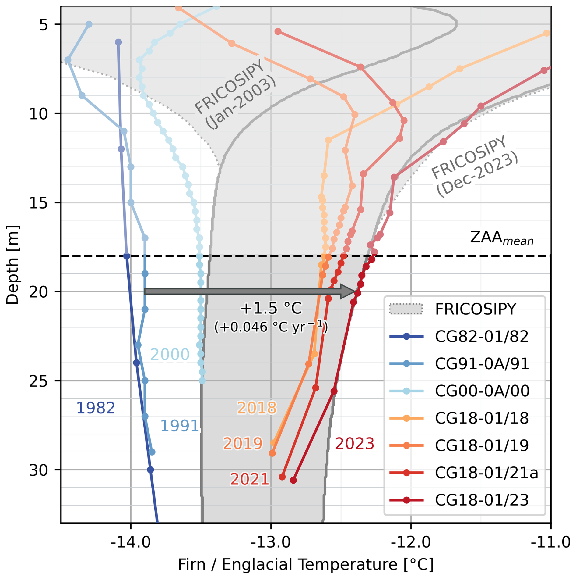
Figure 10 Simulated englacial warming at the SP (grey enclosed region), corrected for model temperature bias at the SP of +0.41 °C, compared to observed borehole thermistor profiles (Haeberli and Funk, 1991; Suter et al., 2001; Suter and Hoelzle, 2002; GLAMOS, 2020, 2022, 2024). Borehole thermistor profile codes adhere to the common naming convention described in the caption of Fig. 8. Firn/englacial temperatures below the mean depth of zero annual amplitude (ZAA) are isolated from seasonal variance and considered indicative of long-term climatic changes.

Simulated firn warming by FRICOSIPY is 11 % greater in magnitude (0.051 °C yr⁻¹), with an average temperature bias of +0.41 °C at the SP (Fig. 9). It is noteworthy that this modelled warming is non-linear; it markedly accelerates from 2015 onwards in response to the increase in surface melt and meltwater refreezing showcased in Figs. 5b and 6b respectively. It is, however, challenging to verify this trend owing to a lack of reliable temperature measurements at the SP between 2000 and 2018.

The development of a strong inversion in the thermal gradients of measured profiles beyond the depth of seasonal variation (∼ 18 m) is observed in Fig. 10. From near-steady-state conditions in 1982, a distinctly negative gradient of −0.042 °C m⁻¹ is visible in the most recent “CG18-01/23” profile. Our simulation results, displayed in Fig. 10 (corrected for the model temperature bias at the SP of +0.41 °C), also show an alteration to the thermal gradient in the uppermost 30 m of the firn but considerably overestimate warming beyond 26 m. At the SP, only the “CG82-01/82” profile extends beyond 30 m to the glacier base at a depth of approx. 120 m, where the basal firn temperature tends to −12.3 °C (Haeberli and Funk, 1991). Evidence from more recent deeper thermistor profiles taken towards the Signalkuppe flank (“CG21-01/21”) suggest warming is currently less pronounced beyond 40 m, and, following an inflexion point in the thermal gradient, englacial temperatures continue to increase with depth towards the bedrock (Schwerzmann, 2006; GLAMOS, 2022).

5 Discussion

5.1 Surface energy and mass exchanges

The FRICOSIPY simulation shows a prolongation of the trends in increasing surface melt at CG identified by Mattea et al. (2021) and a strong corroboration with the spatial distribution of melt shown by their simulation using the EBFM (Fig. 5). Nevertheless, our results are not considered fully validatory given the operational similarity between the two applied models – principally with regard to the commonality of parameterisations used to model surface interactions (Table 1). Explicit measurements of melt are deficient at CG; however, Lier (2018) compiled quantitative estimations of the magnitude of refreezing by assessing observed density anomalies from firn cores at CG compared to an ideal dry densification profile. Annual refreezing rates within confidence intervals of 3–33 and 1–13 cm w.e. yr⁻¹ were reported for the Zumsteinkern and Sattelkern, situated at the ZS and SP reference points respectively. A wide variety of cores were analysed on the Signalkuppe flank, with values ranging between 0–16 cm w.e. yr⁻¹; however, none of these are co-located with our SK reference location. These results provide reasonable attestation to our simulated melt quantities (Fig. 5a), given the inherent uncertainties in this technique and the tendency for underestimation as a result of the occurrence of melt–refreeze cycles (Mattea et al., 2021).

There are, however, considerable limitations in the modelling of surface energetics and also in the spatial homogeneity of relative humidity and wind speed in our model meteorological forcing, which may ultimately influence our simulated melt quantities. Fortunately, the sensitivity of the modelled melt output to humidity changes was found to be low, and, regardless, the strong vertical decorrelation observed when comparing high-altitude meteorological stations above 3400 m a.s.l. makes spatial adjustments difficult. In contrast, variations in wind speed are much more impactful, owing to the magnitude to which this meteorological variable controls both sensible and latent energy exchange (Eqs. 11–12) and its high and often unpredictable spatial–temporal variability. At CG, accurately quantifying the spatial variation in wind velocity over the computational domain presents challenges due to the complex interaction between the prevalent high-altitude, large-scale flows and the effects of the local mountainous topography. Conditions on the exposed CG saddle and the summit of the Signalkuppe, where the CM AWS anemometer is positioned, are likely highly different to the more shielded slopes of the lower Grenzgletscher, where localised katabatic winds may be more representative of air flow. Moreover, the assumption of saturated vapour pressure above the glacier for the calculation of the latent heat flux may also lead to a significant overestimation of sublimation, while, in actuality, reported values from field observations indicate that vapour deficits can occur (Schmidt, 1982). Given the strong influence of turbulent exchange at CG (Fig. 4) and the key contribution sublimation has in evacuating energy from the surface from a high-altitude accumulation area of a glacier, improved modelling of these processes is vital to ensure more accurate estimations of melt.

A recognised shortcoming in the architecture of FRICOSIPY's skin-layer SEB formulation is the decoupling of energy absorption at the surface and the subsequent dissipation of thermal energy via diffusion (Brun et al., 2023). Operating at our hourly temporal frequency, the delay in the evacuation of energy from the surface leads to a potential susceptibility for significant temperature and thus melt overestimates. Brun et al. (2023) reported a 30 % reduction in melt by switching to a 1 min time step for the simulation of an ablating ice surface and also a high sensitivity to the selection of the subsurface heat flux parameters (z_{interp 1 & 2}). However, investigations using our model with a temporally downscaled version of our meteorological time series at 1 min intervals produced less than a 7 % variation in melt at the SP. Site differences are suspected to be a principal factor in this discrepancy, as Brun et al. (2023) concluded this problem was most pronounced in the modelling of the ablation of an exposed ice surface. The uninterrupted coverage of low-density snow layers with a weak thermal conductivity throughout the ablation season at CG greatly curtails the contribution of the modelled subsurface heat flux to the SEB at CG (Fig. 4); therefore, the rate of thermal diffusion at the surface is low.

Finally, the significant quantities of surface melt modelled during negative air temperatures at CG further reinforce the importance of using physically based energy balance models to attain accurate estimations of total annual melt. This phenomenon (also simulated by the EBFM; Mattea et al., 2021) was observed locally at Seserjoch over the course of several days of sub-zero temperatures over the summer of 1999 (Suter et al., 2004). As such, more simplistic approaches, such as degree-day models (e.g. Hock, 1999), may be limited in their application to high-alpine locations and the modelling of a cold firn accumulation area.

5.2 Firn temperatures

Modelled firn temperatures show good corroboration with in situ measurements and the previous modelling efforts of Mattea et al. (2021), showcasing the strong aspect and elevation-dependent gradients at CG previously established by Suter and Hoelzle (2002). However, the exact temperatures have a particularly high sensitivity to the selection and parameter calibration of the preferential percolation scheme of Marchenko et al. (2017) due to its strong influence on the retainment of thermal energy released by meltwater refreezing. Our high-resolution thermistor chains at the SP provide insight into the importance of this process, showing a remarkable increase of 7.74 °C at approximately 4 m depth over the course of 20 d during the summer melt season of 2022 (Fig. S2 of the Supplement). Unfortunately, a malfunction with our on-site ultrasound depth sensor resulted in a high degree of uncertainty on the depth of these measurements (±0.5 m), impeding the full exploitation of these valuable data. Generally, failing to represent preferential percolation by using the default bucket approach of COSIPY was found to result in an underestimation of modelled firn temperatures by as much as 10 °C on the lower Grenzgletscher slope (Fig. A1 of Appendix A). However, the statistical approach used still has considerable limitations: principal among which is the spatially and temporally constant characteristic preferential percolation depth (z_lim). This is a major contributing factor to the underestimation of firn temperatures on the lower Grenzgletscher slope and the Seserjoch; it is simply not possible to represent the entire modelling domain, comprising multiple firn facies, with a single immutable value. In actuality, the percolation depth has been observed to increase over the course of a melt season and is heavily influenced by the supply of meltwater (Marchenko et al., 2017) and by historic infiltration and refreezing events which affect the firn's stratigraphy (Illangasekare et al., 1990).

Alternative physically based preferential percolation schemes are generally derived by resolving the Richards equation or the simplified Darcy's law but are typically computationally expensive (Short et al., 1995; Vandecrux et al., 2020). An estimation of grain size is also required to derive the preferential flow channel area (Katsushima et al., 2013), but in situ quantitative data on snow and firn microstructure are scarce. Wever et al. (2014) implemented a dual-domain approach into the SNOWPACK model (Bartelt and Lehning, 2002), whereby the pore space can be subdivided into both matrix and preferential flow; however, its implementation into FRICOSIPY would require a complete redesign of the subsurface model, and there is no guarantee that more sophisticated physically based methods would necessarily yield more accurate results. Verjans et al. (2019) noted that the performance of the Wever et al. (2014) method did not always supplant a single domain Richard's equation scheme or a standard bucket approach. Nonetheless, while the implementation of these more advanced methods certainly is feasible, their functionality would be limited without suitable calibration data; the acquisition of which remains the foremost priority for future research.

The dimensionality of FRICOSIPY is also a further constraint for the accurate representation of percolation in general, as flow is rarely confined solely to the vertical direction; in areas of steep inclination, gravitational forces will induce lateral movement down-slope. Furthermore, the formation of ice lenses from historic meltwater refreezing events can lead to the development of low-permeability barriers to the downward percolation of water, forcing lateral flow as a consequence. The firn ultimately develops a complex and highly irregular stratigraphy over time, with multiple impedances to meltwater flow forming (Machguth et al., 2016; Clerx et al., 2022). Thus, truly accurate modelling of percolation would require a fully three-dimensional spatial model.

Variation between observed and simulated firn temperatures could also be attributed to physical processes not represented in the FRICOSIPY model. The eastern flank of the saddle and the Signalkuppe comprises a strongly insolated vertical rockwall, measured by Gruber et al. (2004) to have a mean annual ground surface temperature (MAGST) of −5.4 °C in 2001. Assuming basic one-dimensional heat conduction through ice, the four profiles of the “CG05-01” borehole that are located 150 m away could be subject to a lateral heat flux of 0.1 W m⁻² – significantly greater than the prescribed vertical basal heat flux of 0.040 W m⁻² and potentially influential in the model's underestimation of temperatures on the periphery of the Signalkuppe slope (Fig. 8). Further three-dimensional effects such as heat advection are also not considered. Whilst measured surface velocities around the SP are small at a magnitude of 1–3 m yr⁻¹, these increase on the southeastern reaches of the saddle with an acceleration of ice flow moving down onto the steeper slopes of the lower Grenzgletscher (Licciulli et al., 2020).

Consideration should also be given to the reliability of englacial temperature measurements when assessing model performances, as measured values may be subject to significant uncertainty or error. Measurements at CG prior to 2018 were conducted using an analogue thermistor chain lowered into the glacier for up to 12 h, often providing insufficient time to fully equilibrate with the surrounding firn/ice. The final temperatures would therefore be estimated based on the extrapolation technique of Lachenbruch and Brewer (1959), typically achieving an accuracy in the order of ±0.1 °C (Suter et al., 2001). However, closer to the surface, firn temperatures are closely coupled to the highly variable meteorological conditions and are susceptible to processes that transcend the surface, such as wind pumping (Clarke et al., 1987). Furthermore, several measurements in our validation dataset are suspected to be significantly influenced by the thermal perturbations from steam drilling that had yet to fully dissipate. These factors may be just as influential in explaining discrepancies between simulated and observed temperatures profiles as limitations in the model.

Spatially, model output sensitivity is significantly greater in the southwestern reaches of the computational domain, particularly with regard to firn temperatures (Appendix B). These lower-altitude, heavily insolated areas are subject to greater meltwater production (Fig. 5a), and, as such, domain-wide adjustments to the model have considerably larger implications on the magnitude and retainment of latent heat release from refreezing – ultimately manifesting in greater firn temperature variance. The spatial extent of the cold-temperate firn transition displayed in Fig. 7a is therefore subject to a large degree of uncertainty. The tuning of key model parameters based on conditions at the CG saddle and the dense concentration of validation data inevitably causes a systematic bias away from this area, further exacerbating this issue. Accurately demarcating firn facie boundaries and their temporal evolution would therefore require a computational domain encompassing a more complete range of topographic expositions across altitudes between 3800 and 4600 m a.s.l. and a better-distributed validation set – akin to the research of Suter and Hoelzle (2002).

5.3 Firn warming

With regard to firn warming at CG, while this is undoubtedly strongly associated with the observed trend in increasing MAAT (Fig. 9), there are significant limitations using this metric to assess firn changes. Given that melt occurs almost exclusively during the summer at CG and given the profound influence it has on the thermal regime, the summer air temperature is fundamentally much more indicative of deep-firn temperature evolution than the annual mean. In our simulation, the MASAT has been demonstrated to strongly correlate with annual melt and subsequent firn warming (Figs. 5b and 6) in comparison to the MAAT – a Pearson correlation coefficient of 0.90 compared to just 0.63. The meltwater infiltration re-crystallisation process enables energy to bypass the thermally insulating near-surface firn layers that effectively decouple deep-firn temperatures from extreme conditions at the surface. As such, firn temperatures at CG are much more sensitive to small variations in summer melt than any extreme meteorological conditions found throughout the remainder of the year. This is the principal reason why our model spin-up was based on a reconstruction of monthly air temperatures, to ensure our meteorological data were representative of seasonal conditions prior to 2003.

It is evident from our investigation that small alterations in the meteorological data used in the model spin-up have a strong influence on the magnitude of modelled firn warming (Fig. 9), sometimes of greater significance than major changes to the parameterisations of the model's physical processes. Initialising the model to accurate steady-state conditions is an important pre-requisite to prevent a transient response during the initial time period of any simulation. In our case, preliminary simulation runs using a spin-up based on eight loops of the 2004–2011 CM AWS meteorological data (as used by Mattea et al., 2021) initialised firn temperatures 0.48 °C higher in 2003, leading to limited warming in the first 11 years of the simulation, as seen with the EBFM. The thermal profile beneath the zero annual amplitude (ZAA) would also initialise in a steady-state condition – similarly to the “CG82-01/82” profile (Fig. 10). In actuality, the subsurface thermal regime at CG has not been in equilibrium since the 1980s and is continually evolving in response to atmospheric warming at the surface over the previous 4 decades (Haeberli and Funk, 1991; Lüthi and Funk, 2001a), leading to the prominent thermal gradient inversion shown from measured profiles in Fig. 10. These considerations compelled to us to replace the former model spin-up with one with meteorological conditions representative of the mid-late 20th century and to extend the simulation depth of the original study from 20 to 50 m, in order to accurately initialise the subsurface layers of the model. It is therefore our recommendation that great consideration should be given to the accuracy of the model spin-up and the resulting initial conditions, particularly when modelling changes to the thermal regime of firn.

5.4 Future firn evolution at Colle Gnifetti

The observation of a near-linear trend of increasing englacial temperature measurements over the course of 30 years may suggest a prolongation of currently observed trends when predicting the evolution of firn temperatures at CG (Fig. 9). However, there is a significant gap of reliable measurements between 2000 and 2015, and our simulation results suggest a significant acceleration in firn warming following this time period. Indeed, the much greater simulated warming at the lower-altitude Seserjoch and Grenzgletscher may be a better indicator of future conditions at CG – especially with the strong trend in MAAT observed from the CM AWS in recent years. Interestingly, at the Col du Dôme site of the Mont Blanc massif (4250 m a.s.l.), following a warming of 2 °C between 1994 and 2010, near-surface temperatures actually showed a significant cooling up to the latest measurement in 2017 (Vincent et al., 2020). This was primarily attributed to a slowdown in the air temperature warming rate observed from the Lyon-Bron meteorological data series between 1998 and 2015, indicative of the so-called “global warming hiatus” (Meehl et al., 2014), which may also explain the reduced firn warming modelled at CG prior to 2015. Vincent et al. (2020) also suggested that cooling at these lower elevations (compared to CG) could be influenced by the formation of low-permeability ice layers that limit the percolation depth of meltwater and consequently the retainment of latent heat release from refreezing. With our trend of increasing surface melt and evidence of small ice lenses already being observed by Mattea et al. (2021) in 2019, the establishment of such a negative feedback affecting future englacial temperature change at CG is also a distinct possibility. It is also evident that this further reinforces the importance of employing a more sophisticated percolation scheme in order to accurately simulate the evolving thermal regime in a cold firn region.

6 Conclusions

Our research shows that there is considerable potential for using our FRICOSIPY model to accurately model the evolution of cold firn in complex mountainous topography. However, this could only be achieved following significant modifications to several of the model's parameterisations for key physical processes. Significant contributions from our research have already been implemented into the latest v2.0 release of the original COSIPY model.

The FRICOSIPY results show good agreement with the spatial patterns of observed firn temperatures around Colle Gnifetti and a prolongation of a previously identified trend in increasing surface melt (Mattea et al., 2021). This influx of additional meltwater and the resulting latent heat release from refreezing at depth lead to the simulation of firn warming at a rate of 0.051 °C yr⁻¹ at the saddle point, which is comparable to in situ measurements. The simulation also suggests a considerable acceleration in the rate of warming since 2015, in line with increasing air temperatures observed at the Capanna Margherita station. Around the lower-altitude areas of Seserjoch and lower Grenzgletscher (∼ 4300 m a.s.l.), simulated warming is much greater than the local rate of atmospheric warming, resulting in a rapid transition from cold to temperate firn – potentially indicative of future conditions to be expected at the saddle point of Colle Gnifetti. However, owing to the scarcity of validation data and the model's sensitivity in this area, there is significant uncertainty in the model output result.

The study mainly reveals the challenges of accurately modelling firn facie transition, as small changes in the parameterisations of the subsurface model can lead to large temperature variance. In particular, accurately quantifying the refreezing depth of infiltrating meltwater is pivotal in controlling the retainment of thermal energy within the firn. While a variety of viable percolation schemes exist, their performance can be highly variable and their implementation can be constrained by a model's architecture and access to site-specific calibration data. The setup and meteorological data used for the model spin-up are also found to be of profound importance, particularly when analysing the evolution of the subsurface thermal regime in firn.

Appendix A: Baseline COSIPY v1.4 simulation results

Figure A1 shows a comparison between the baseline simulation results using the COSIPY v1.4 model (Sauter et al., 2020), with all default parameters and parameterisations selected, and our modified FRICOSIPY simulation. Firn temperatures and density profiles differ greatly from our results and site measurements – particularly on the lower Grenzgletscher, where there is a deviation in excess of 10 °C (Fig. A1i).

The deficiency for the deep firn to retain thermal energy in the default COSIPY model setup may principally be attributed to the inability of meltwater to percolate to significant depths prior to refreezing and the thermal conductivity of subsurface layers. Without a means to simulate preferential percolation, a process known to be highly influential in the thermal regime of a cold infiltration firn facie (Gascon et al., 2014; Marchenko et al., 2017), percolating meltwater rarely refreezes below 1 m depth. Latent energy release therefore occurs within close proximity to the surface and is highly susceptible to rapid dissipation and loss (Fig. A1ii). This is further exacerbated by a significant overestimation of subsurface-layer thermal conductivity by the bulk volumetric approach (Eq. 22) used in COSIPY compared to data from field and laboratory experiments (Schneebeli, 1995; Giese and Hawley, 2015) and widely used empirical formulations (Sturm et al., 1997; Calonne et al., 2019). Combined with the large positive bias in subsurface-layer density (Fig. A1iii), this leads to the entire simulated depth being strongly thermally coupled to the surface, with deep-firn temperatures tending towards the MAAT. It is unclear what the principal cause behind the large discrepancy between modelled and observed density is; however, we noted a high sensitivity to the selection of the subsurface re-meshing algorithm: whether the default logarithmic or adaptive Lagrangian methods of COSIPY or our fixed Lagrangian approach. There could also be a location-specific incompatibility with employing the Boone (2009) firn densification scheme, as these parameterisations have been found to have considerably variable performance at different sites (Lundin et al., 2017).

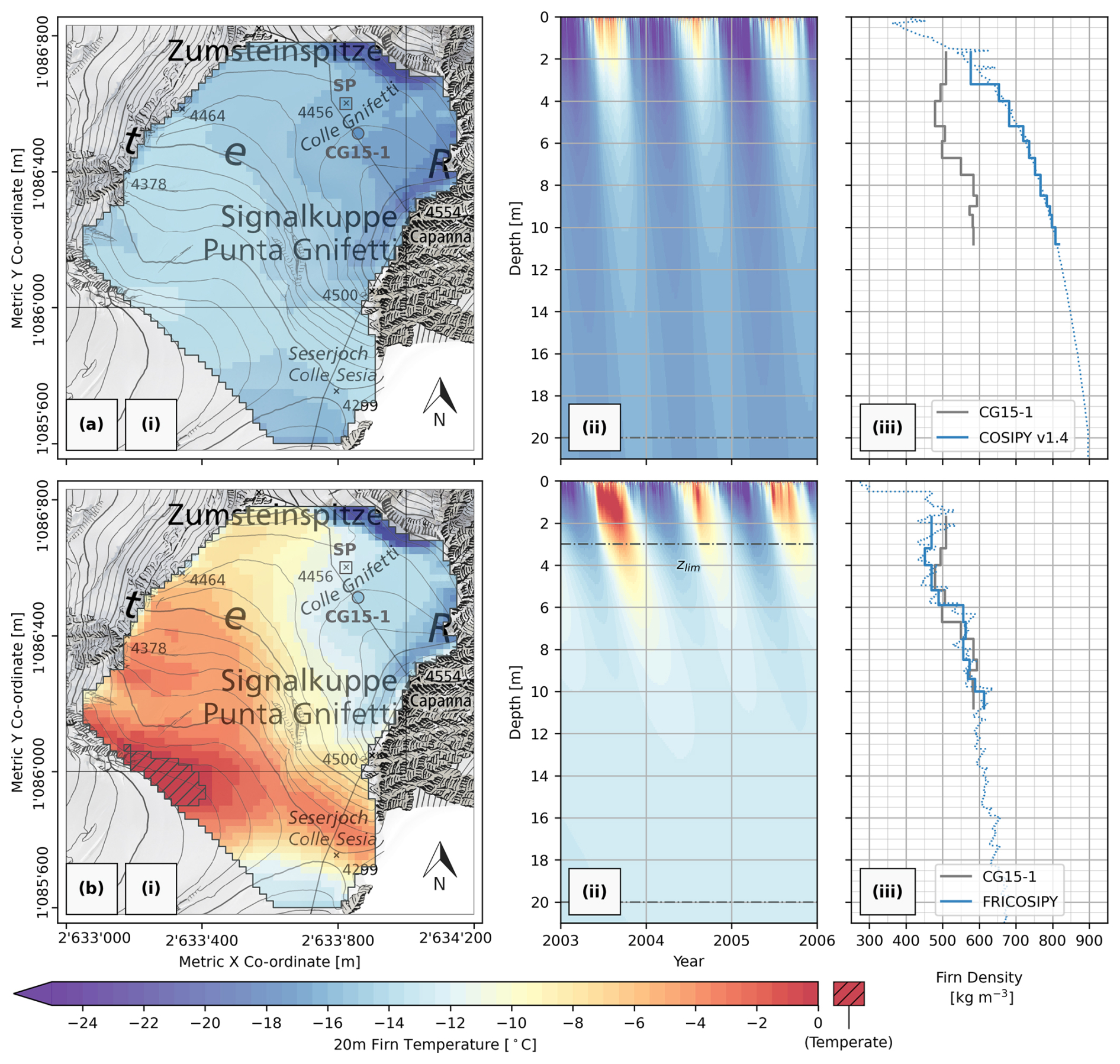
Figure A1 (a) Baseline COSIPY v1.4 using the default parameter set compared against (b) our modified FRICOSIPY simulation results. (i) Modelled 20 m depth firn temperatures at the simulation end date of 31 December 2023, (ii) modelled firn temperature–depth profile at the SP (2003–2006), and (iii) modelled density–depth profile compared against the CG15-1 firn core (27 September 2015) (GLAMOS, 2020; Banfi and De Michele, 2022). Spatial co-ordinates are defined by EPSG 2056 (Metric Swiss CH1903+/LV95). Topographic map and orthoimage sources: Swisstopo (2017, 2023).

Appendix B: Model sensitivity study

As part of our research, a thorough sensitivity study was conducted to better understand the influence of parameter adjustment on model output, with a particular focus on understanding the effect of modelled firn temperatures. Figure B1a shows the influence of changing the most sensitive parameters and parameterisations from the values selected in Tables 2 and 3 on the 20 m firn temperature at the SP. These are principally those that either significantly alter the magnitude of surface melt or influence heat transfer in the subsurface. For the former, modifying the fresh snow albedo (α_snow) impacts the net shortwave radiation absorbed by the surface (Eqs. 4–6), while changing the surface roughness (μ) alters the turbulent exchange coefficient (Eqs. 12–14) and ultimately the magnitude of latent exchange via sublimation – an important endothermic process that expends energy that would otherwise be allocated to melt. In the latter case, altering the thermal conductivity (k) controls the rate of thermal diffusion: either directly by changing the parameterisation for thermal conductivity to an alternative such as that of Sturm et al. (1997) or indirectly by modifying the firn density of subsurface layers (ρ_snow), which the model uses to define their thermal conductivity (Eq. 22 or Eq. 26). Finally, altering the characteristic preferential percolation depth (z_lim) of the Marchenko et al. (2017) parameterisation (Eqs. 28–29) controls the depth at which energy is released by refreezing and thus the extent to which it is retained in the subsurface.

Across the wider modelling domain, firn temperature changes induced by parameter or parameterisation selection generally always adhere to the prevailing spatial patterns – these are predominantly defined by nodal topography and accumulation and are rarely influenced by modifying the model processes. Moreover, model output sensitivity holds a strong Pearson's correlation of 0.92 to the firn temperature of a given node, with areas at the cold-temperate transition (∼ 0 °C) being the most sensitive to changes (Fig. B1b). In these regions, parameter changes induce the strongest changes in the quantity of surface melt production and also the magnitude and retainment of latent heat release from refreezing, leading to the greatest firn temperature variance. Conversely, areas on the northern periphery of CG that the simulation models as a cold re-crystallisation zone (Fig. 5a) are extremely insensitive to changes; the absence of melt causes a very weak coupling with surface iterations and the meteorological forcing, leading to the firn temperatures being largely invariable from the baseline. Intuitively, one can also surmise that, if lower-altitude, permanently temperate areas of the Grenzgletscher were modelled, these would also be relatively insensitive to change. Hence, this sensitivity study suggests that, in modelling the thermal regime of a polythermal glacier, uncertainty will likely always be greatest at the cold-temperate firn transition, due to the inherently high sensitivity this area holds to the calibration and parameterisation of a model's physical processes.

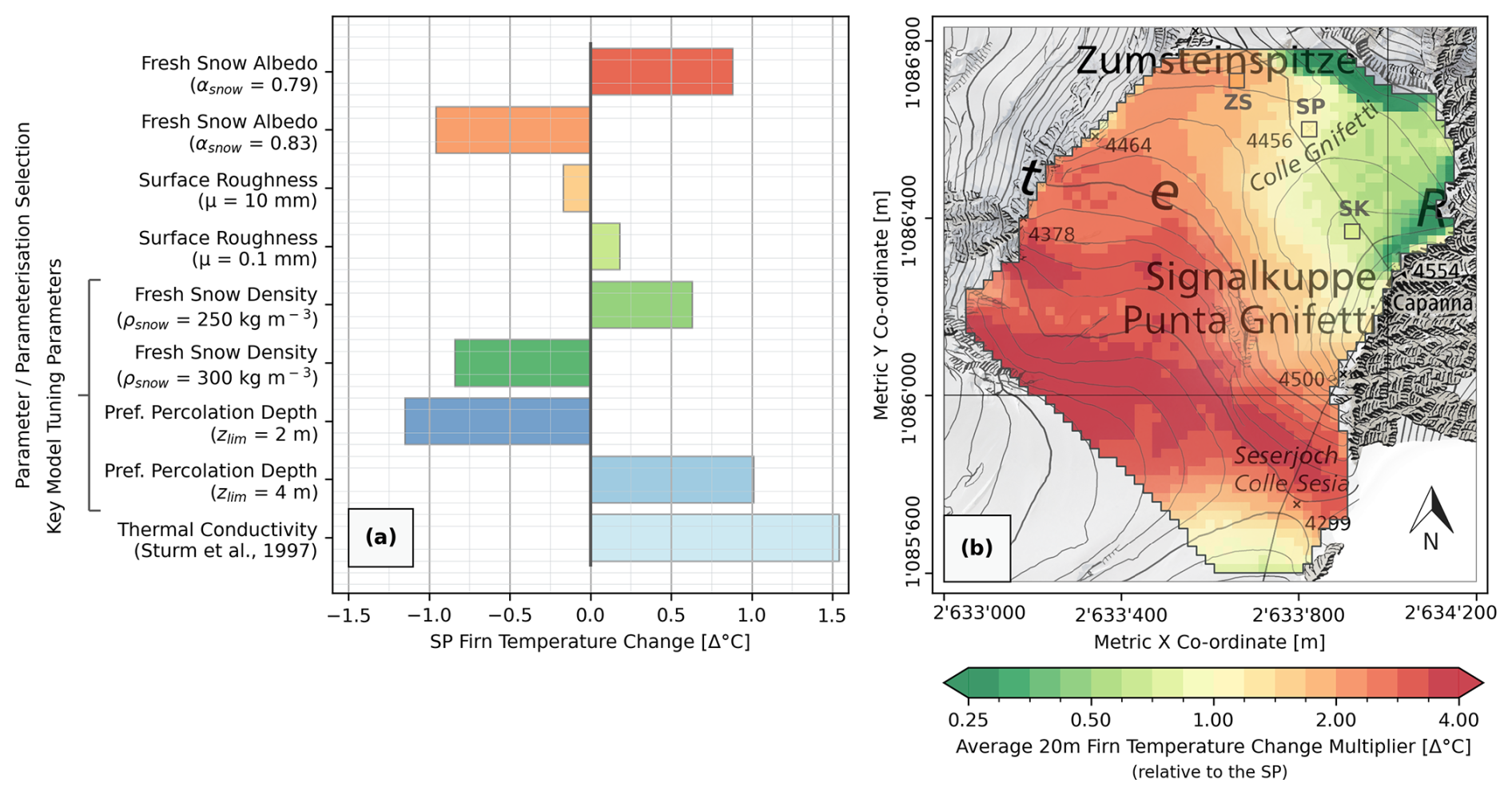
Figure B1 Model sensitivity study overview showcasing the implications of adjusting the most sensitive parameters or parameterisations from the values selected in Tables 2 and 3 on (a) the 20 m firn temperature at the SP and (b) the average change in 20 m firn temperature relative to the SP across the wider spatial domain – not considering physical constraints on temperature (T≤0 °C). For example, if adjusting a given parameter increases the 20 m firn temperature at the SP by 1 °C, an increase of approximately 2 °C can be expected at the ZS. Spatial co-ordinates are defined by EPSG 2056 (Metric Swiss CH1903+/LV95). Topographic map and orthoimage sources: Swisstopo (2017, 2023).