Radar-equivalent snowpack: reducing the number of snow layers while retaining their microwave properties and bulk snow mass

Snow water equivalent (SWE) retrieval from Ku-band radar measurements is possible with complex retrieval algorithms involving prior information on the snowpack microstructure and a microwave radiative transfer model to link backscatter measurements to snow properties. A key variable in a retrieval is the number of snow layers, with more complex layering yielding richer information but at an increased computational cost and number of unknowns. Here, we show the capabilities of a new method to simplify a complex multilayered snowpack to two to three layers while nearly preserving the microwave scattering behavior of the snowpack and conserving the bulk snow water equivalent. This method, called radar-equivalent snowpack, is based on a k-means clustering algorithm to group the snow layers based on the extinction coefficient and a weighted average using the optical thickness applied to the snow properties. We evaluated our method using snow properties from simulations of the Soil, Vegetation and Snow version 2 (SVS-2)/Crocus physical snow model at 11 sites spanning a large variety of climates across the world and the Snow Microwave Radiative Transfer model to calculate backscatter at 17.25 GHz. The layer simplification is done as an intermediate step between the physical modeling (SVS-2/Crocus) and the microwave radiative transfer (Snow Microwave Radiative Transfer Model – SMRT). Grouping and averaging snow stratigraphy into three layers effectively reproduced the total snowpack backscatter of multilayered snowpacks, with an overall root mean squared error of 0.5 dB and R²=0.98. Using this methodology in SWE retrieval applications, this method can be used to simplify snowpacks and reduce the number of variables to optimize while maintaining similar scattering behavior without compromising the modeled snowpack properties. A reduction in the mathematical complexity of SWE retrieval cost functions and a reduction in computation of up to 80 % can be gained by using fewer layers in the SWE retrieval.

1 Introduction

Snow water equivalent (SWE) is a key element of the hydrological cycle and an important component of the surface energy balance, so it must be well-represented in environmental prediction systems. Because conventional SWE observations are exceptionally sparse, new spaceborne radar missions to deliver SWE information are under development, such as the Canadian Terrestrial Snow Mass Mission (TSMM, Derksen et al., 2021; Tsang et al., 2022). A state-of-the-art SWE retrieval from the Ku-band radar measurements delivered by a mission like TSMM requires a radiative transfer model (RTM) to link snow properties to backscatter (Saberi et al., 2021; Zhu et al., 2021; Pan et al., 2017, 2024). Snow properties, including layer thickness, density, temperature, and microstructure (e.g., specific surface area), are necessary to model the microwave signal with an RTM properly. Prior or first-guess information on layered snow properties is needed to constrain retrievals (Merkouriadi et al., 2021; Durand et al., 2024). This information can come from vertical snowpack measurements, either manually or using an instrument like a high-resolution snow penetrometer (SMP, Proksch et al., 2015). More typically, observations are unavailable, so snowpack information can come from physical snow models that provide multilayered snow properties based on meteorological forcing data.

Detailed physical snow models like Crocus (Vionnet et al., 2012) and SNOWPACK (Bartelt and Lehning, 2002; Lehning et al., 2002) are one-dimensional multilayered physical schemes that can model the evolution of the snowpack (including its microstructure) by taking into account energy exchange between the snow, the atmosphere, and the soil based on meteorological inputs. In Crocus, the snowpack is vertically discretized on a finite-element grid with specific rules to allow the snowpack layering to evolve dynamically from new precipitation, compaction, and/or metamorphism. One such rule is the dynamic attribution of the number of layers and thicknesses to simulate the snowpack layering. The minimum number is 3 layers, but the maximum is 50 (Vionnet et al., 2012). Numerical snow models that use large numbers of layers can improve the representation of dynamic physical processes within the snowpack, such as heat and mass fluxes, resulting in a better representation of the temperature profile. Better simulation of the vertical temperature profile within the snow improves the simulation of microstructure evolution and spring snowmelt initiation (Cristea et al., 2022). Therefore, there is a benefit to adding layers in physical modeling to improve the full vertical profile of snow properties.

Some algorithms couple a physical snow model and a snow RTM to retrieve SWE using microwave remote sensing data (Langlois et al., 2012; Larue et al., 2018; Singh et al., 2024). Snow RTMs can model the radar backscatter using snow parameters from complex layered snowpacks. In a SWE retrieval like in Pan et al. (2017), the SWE (a function of depth and density) of the different layers is estimated by minimizing the difference between the modeled and measured backscatter. To simulate the backscatter, most RTMs solve the radiative transfer equation based on the discrete ordinate and eigenvalue method (Picard et al., 2004), which discretizes the radiative transfer equation and solves a nonhomogeneous system of linear equations based on the number of layers. Increasing the number of snow layers thus increases the computational cost at many levels within the retrieval algorithm. Also, a larger number of layers increases the complexity of the retrieval by increasing the number of variables in the cost function. This is why current retrievals typically use a two-layer model (Saberi et al., 2021; Pan et al., 2017). Completely neglecting stratigraphy by using a one-layer model can affect the performance of the retrieval (Durand et al., 2011) because layering strongly influences the backscattering properties of snow (Rutter et al., 2016). A one-layer model oversimplifies the scattering behavior of the snowpack and so is not adequate in most cases (Rutter et al., 2019; Meloche et al., 2024; Montpetit et al., 2024). For this reason, a two- or three-layer model provides notably better SWE retrievals by accounting for stratigraphy in a certain way (Pan et al., 2017; Saberi et al., 2021). In the end, there is a disconnect between needing several layers in a physical model to simulate a realistic microstructure profile and needing only two or three layers in SWE retrievals for computation simplicity.

To reduce the number of layers, a mass- or thickness-weighted average is commonly used to average all properties of the snowpack (Durand et al., 2011) and conserve snow mass (i.e., SWE). Singh et al. (2024) applied the same logic in averaging a multilayered snowpack into a two-layer snowpack and chose the height that corresponded to the maximum change in density to split the snowpack into two layers. Other SWE retrievals (Saberi et al., 2021) focused on arctic snowpacks by setting the initial two-layer snowpack from well-documented layer properties (e.g., wind slab and depth hoar for Arctic snowpacks) (Rutter et al., 2019; Vargel et al., 2020; Derksen et al., 2009, 2012). For assimilation of passive microwave data, Larue et al. (2018) used a detailed physical snow model (Crocus) coupled with an RTM with a limit of 15 layers as a compromise between accuracy and computation time. Yu et al. (2021) proposed an interesting method for estimating an effective one-layer snowpack for passive microwave applications that calculates a SWE-weighted average for the microstructure parameter and preserves the reflectivity of the air–snow and snow–ground interfaces from the multilayered snowpack. With this approach, the scattering properties are better preserved. To our knowledge, a robust method still does not exist to effectively reduce the number of layers of a given snowpack while minimizing changes in scattering properties. This would allow the accuracy of the SWE retrieval not to be compromised and the computation time to be reduced.

The goal of this paper is to develop a simple algorithm to convert a multilayered snowpack with a large number of layers (20–50) into a simplified snowpack (2–3 layers) that preserves its snow mass and scattering behavior, thereby improving the computational cost with minimal impact on performance. The method should preserve backscatter within 1 dB, since it is the calibration uncertainty of most synthetic aperture radars (Schmidt et al., 2018). This study only focuses on evaluating our snowpack reduction method on dry snow in the context of SWE retrievals based on volume scattering. However, this method could potentially be used for wet snow since the extinction coefficient would be sensitive to liquid water via the absorption coefficient if the physical model correctly estimates the melt. To evaluate our method, we test it on multilayered Crocus simulations at 11 sites across various snow climates and multiple seasons. From the 50-layer simulations (maximum layering), we compare various methods to obtain a radar-equivalent snowpack by evaluating differences in snow masses and simulated backscatter using the Snow Microwave Radiative Transfer Model (SMRT, Picard et al., 2018).

2 Methods

2.1 Study site and data

A total of 11 sites were selected to cover a wide range of snowpack conditions and climates, and meteorological forcing and evaluation datasets were previously published. Of the 11 sites, 6 are in mountain environments (Col de Porte, Kühtai, and Weissfluhjoch in the European Alps and Reynolds Mountain, Senator Beck, and Swamp Angel in the western USA), 2 are in tundra environments (Bylot and Trail Valley Creek in the Canadian High Arctic), 2 are in taiga environments (Umiujaq in the Canadian boreal forest and Sodankylä in the Finnish boreal forest), and 1 is in a maritime climate (Sapporo in Japan). Details of each dataset are shown in Table 1.

Domine et al. (2021)Menard and Essery (2019)Krajči et al. (2017)Menard and Essery (2019)Menard and Essery (2019)Menard and Essery (2019)Menard and Essery (2019)Menard and Essery (2019)Tutton et al. (2024)Lackner et al. (2024)Menard and Essery (2019)

Table 1 Overview of the sites used to evaluate the Crocus snowpack layering reduction methods.

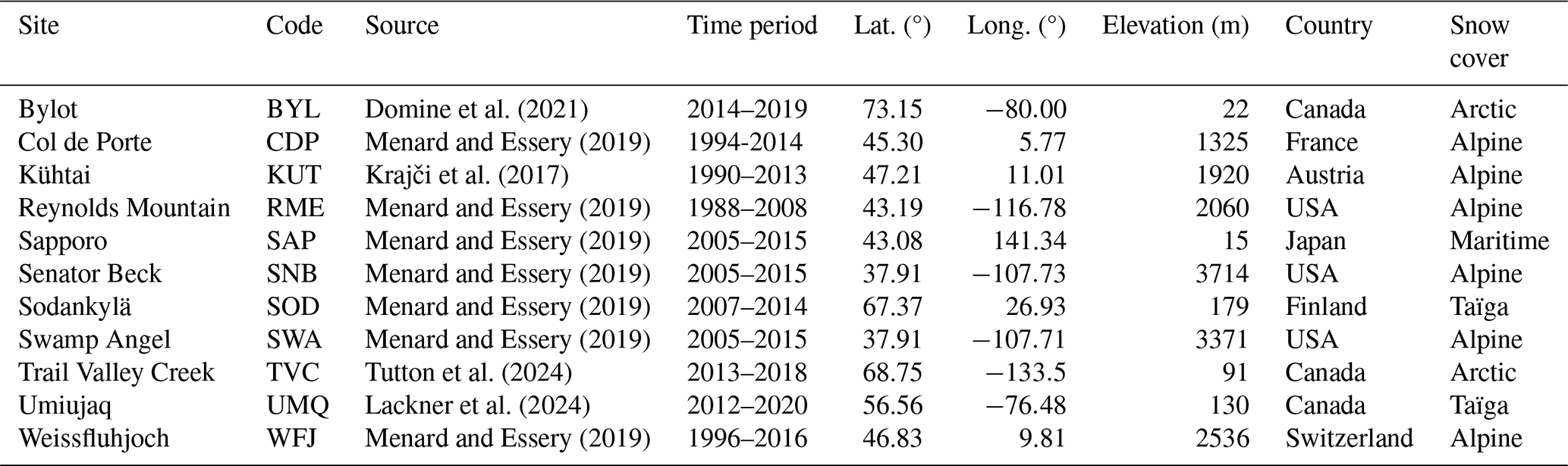
Of the 11 sites, 3 were selected to more easily illustrate the methodology. These sites (TVC, WFJ, and SAP) have distinct snowpack characteristics. The TVC arctic snowpack is characterized by a layer of highly scattering depth hoar with a dense wind slab on top. The WFJ alpine snowpack is characterized by a deep snowpack with a progressive density increase from top to bottom and some melt–freeze crusts due to warming events throughout the season. The SAP snowpack is characterized by a similar alpine snowpack but is more impacted by wet precipitation.

2.2 Soil, Vegetation and Snow version 2 (SVS-2)/Crocus

The snowpack model Crocus (Brun et al., 1992; Lafaysse et al., 2017; Vionnet et al., 2012) was used to simulate the evolution of the snowpack properties, i.e., the number of layers, thickness, density, liquid water content, temperature, and specific surface area for each layer. The version of Crocus used in this study is implemented in the SVS-2 land surface scheme (Garnaud et al., 2019; Vionnet et al., 2012; Woolley et al., 2024). The snowpack model is coupled to a multilayered soil model that includes soil freezing and thawing (Boone et al., 2000). SVS-2 is an improvement to the SVS land surface scheme (Alavi et al., 2016; Husain et al., 2016; Leonardini et al., 2021) used at Environment and Climate Change Canada for hydrological prediction. For the simulations at the arctic sites (Bylot and Trail Valley Creek), the Arctic version of Crocus (Royer et al., 2021b; Woolley et al., 2024) was used. This version improves the simulation of the wind slab properties and includes the impact of basal vegetation on snowpack properties. This allows a better “arctic” density profile by increasing the wind slab density and lowering the depth hoar density.

At each site, simulations were run with a maximum number of 50 snow layers. Table B1 summarizes the options of Crocus for each physical process and the snow aging parameters (Gaillard et al., 2025) used for the simulations at the different sites. At the two Arctic sites, the polar vegetation height was set to 10 cm (Woolley et al., 2024), and for the taiga sites it was set to 50 cm and 20 cm for UMQ and SOD, respectively. The model uses a time step of 10 min, and the meteorological forcing is provided hourly.

2.3 SMRT

SMRT is a multilayered snow radiative transfer model that can compute backscatter in the microwave range. It considers each snow layer to be a homogeneous random medium composed of air and ice and solves the radiative transfer equation for a multilayered snowpack (Picard et al., 2018). Each snow layer is represented by temperature, density, thickness, and microstructure parameters, all of which are provided by Crocus. One key component of SMRT is determining the scattering and absorption coefficients (κ_s and κ_a) of each layer. These coefficients dictate the radar scattering and absorbing behavior of the medium (snow). For snow, this generally implies that scattering (κ_s) dominates for dry snow and that absorption (κ_a) dominates for wet snow. The extinction coefficient (${\mathit{\kappa }}_{\mathrm{e}}={\mathit{\kappa }}_{\mathrm{s}}+{\mathit{\kappa }}_{\mathrm{a}}$) characterizes the interaction within the medium by accounting for both coefficients and is a key parameter of the snow layer reduction algorithm presented in this paper. Multiple formulations of the coefficients can be used depending on the electromagnetic model, but here we focus on the improved Born approximation (IBA, Mätzler, 1998) implemented in SMRT.

The phase function of snow in the 1–2 frame, e.g., ice particles (medium 2) in an air matrix (medium 1), is defined by

$$\begin{array}{}\text{(1)}& \begin{array}{rl}{p}_{\text{1–2 frame}}& (\mathit{\vartheta },\mathit{\phi })={\mathit{\varphi }}_i(\mathrm{1}-{\mathit{\varphi }}_i)({\mathit{ϵ}}_{\mathrm{2}}-{\mathit{ϵ}}_{\mathrm{1}}{)}^{\mathrm{2}}{Y}^{\mathrm{2}}({\mathit{ϵ}}_{\mathrm{2}},{\mathit{ϵ}}_{\mathrm{1}})k_{\mathrm{0}}^{\mathrm{4}}\\ & M\left(\right|k_d\left|\right){\sin }^{\mathrm{2}}\mathit{\chi },\end{array}\end{array}$$

where k₀ is the wavenumber in free space and ϕ_i is the volume fraction of the scattering constituent (ice) describing ${\mathit{\varphi }}_i={\mathit{\rho }}_{\mathrm{snow}}/{\mathit{\rho }}_{\mathrm{ice}}$, with ρ_snow the snow density (kg m⁻³) and ρ_ice the pure ice density (kg m⁻³). ϵ is the relative permittivity of both media, and χ is the polarization angle defined by ${\sin }^{\mathrm{2}}\mathit{\chi }=\mathrm{1}-{\sin }^{\mathrm{2}}\mathit{\vartheta }{\cos }^{\mathrm{2}}\mathit{\phi }$ for the scattering (ϑ) and incident (φ) directions. The mean square field ratio (Y²) accounts for the difference in the electric field between the background and scattering media (see Picard et al., 2018, for the equations). The microstructure term ($M\left(\right|k_d\left|\right)$) is defined by the Fourier transform of the autocorrelation function (ACF) of the medium. Here, we used the exponential model (Mätzler, 2002), where the ACF is characterized by a correlation length (l_mw) estimated by the specific surface area (SSA) and the snow density. More details on the ACF and $M\left(\right|k_d\left|\right)$ can be found in Picard et al. (2018). κ_s can be calculated from the following equation:

$$\begin{array}{}\text{(2)}& {\mathit{\kappa }}_{\mathrm{s}}=\mathit{\pi }\underset{\mathrm{0}}{\overset{\mathit{\pi }}{\int }}\left[p_{\mathrm{11}}\right(\mathit{\vartheta })+p_{\mathrm{22}}(\mathit{\vartheta }\left)\right]\mathrm{d}\mathit{\vartheta },\end{array}$$

where $p_{\mathrm{11}}=p_{\text{1–2 frame}}(\mathit{\vartheta },\mathit{\phi }=\mathit{\pi }/\mathrm{2})$ and $p_{\mathrm{22}}=p_{\text{1–2 frame}}(\mathit{\vartheta },\mathit{\phi }=\mathit{\pi })$ are defined by the phase function. κ_a is defined by

$$\begin{array}{}\text{(3)}& {\mathit{\kappa }}_{\mathrm{a}}=\mathrm{2}{k}_{\mathrm{0}}\mathrm{\Im }\left(\sqrt{{\mathit{ϵ}}_{\mathrm{eff}}}\right),\end{array}$$

where ϵ_eff is the effective permittivity using the Polden–van Santen general mixing formula (Sihvola, 1999).

In addition to the simulations using the full number of Crocus snow layers, SMRT was used to simulate the backscatter of the snowpack to evaluate our averaging methods (Sect. 2.4). Crocus provides the layered snow density and SSA to estimate the microwave grain size with

$$\begin{array}{}\text{(4)}& l_{\mathrm{mw}}=K{l}_p=K{\displaystyle \frac{\mathrm{4}(\mathrm{1}-{\mathit{\varphi }}_i)}{{\mathit{\rho }}_{\mathrm{ice}}\mathrm{SSA}}},\end{array}$$

where K is the polydispersity of the microstructure. The polydispersity was assumed to be 0.75 for all of the grain types in this experiment, but future work could include a polydispersity for different Crocus-simulated grain types.

Simulations were first performed at the high Ku-band (17.25 GHz), the TSMM frequency that is most sensitive to volume scattering (Derksen et al., 2021), but later the frequency range X-band to Ku-band was also investigated. Vertical co-polarization (VV) was the focus since horizontal co-polarization (HH) will not be measured as part of TSMM (Derksen et al., 2021). A simple absorber for the background was used (no scattering from the ground is assumed) to only obtain the snow contribution to the modeled backscatter. The incident angle was set to 35° as a typical median value for synthetic aperture radar sensors such as TSMM. The snow layer interfaces were assumed to be flat.

2.4 Algorithm

The algorithm aims to reduce the number of snow layers to two or three relevant layers while preserving SWE and scattering behavior with respect to the reference snowpack (defined as the 50-layer Crocus simulations). The main goal is to develop a robust method to aggregate and average snow layer properties in a microwave SWE retrieval context. Figure 1 shows the general methodology for obtaining a radar equivalent snowpack with reduced layers. The method is divided into two operations applied to layers: grouping and averaging.

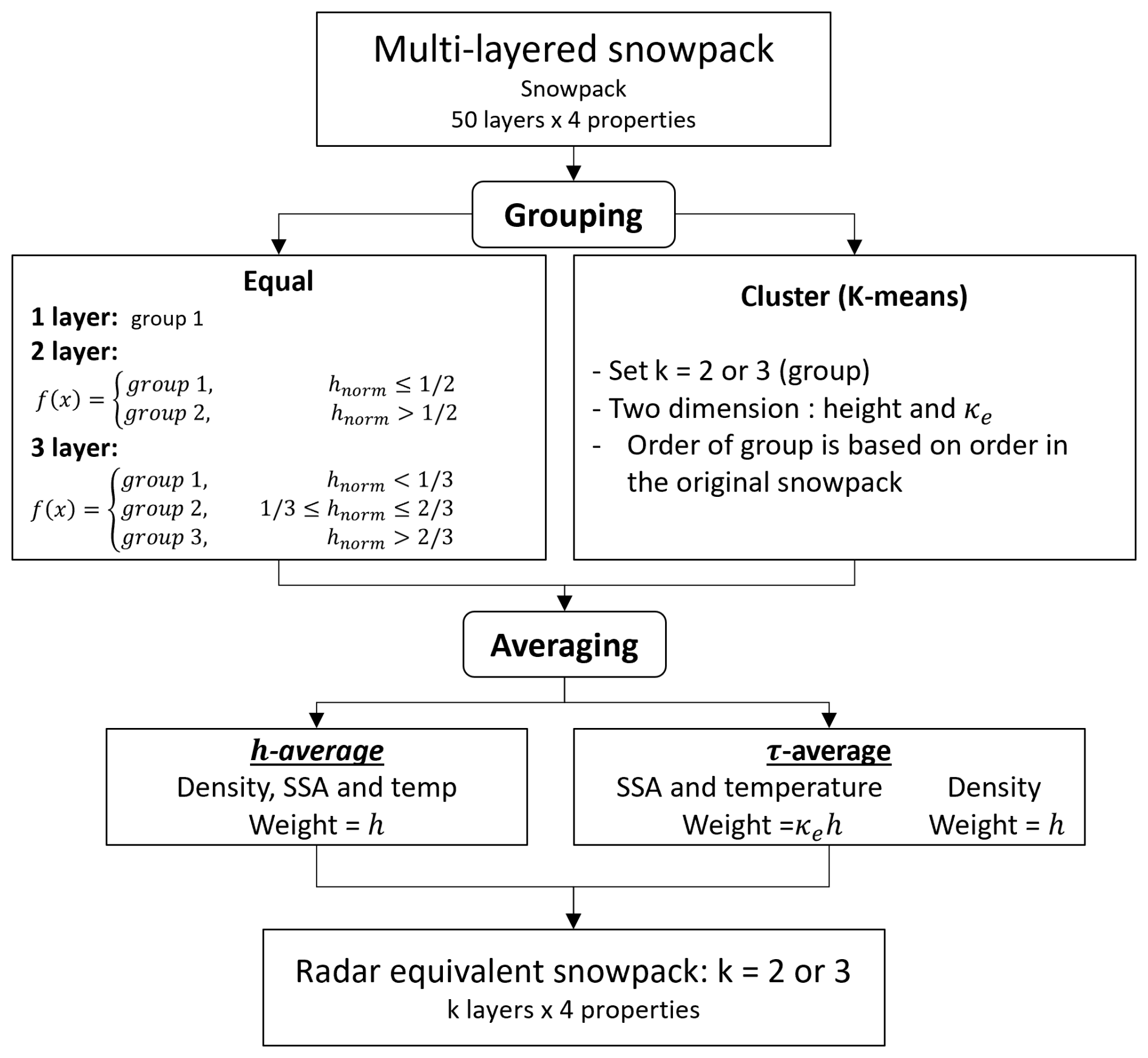
Figure 1 Schematic of the methodology. Necessary steps in the snowpack simplification are shown vertically, and the different options (grouping and averaging) are shown horizontally where h_norm is the normalized height and h is the layer thickness. The four snow properties considered are thickness, density, temperature, and SSA.

The grouping of the layers was done in two ways. The first method was used as a baseline comparison. This method (referred to as equal) aggregated layers based on the normalized height h_norm, which is the height of a layer divided by the thickness of the whole snowpack. For instance, if a snowpack is simplified into two layers, the top half of the snowpack, i.e., all layers with heights greater than one-half of the snowpack thickness, would be aggregated into a first layer and the bottom half would contain all layers with heights that are less than or equal to one-half of the snowpack thickness. This method is a basic way of obtaining an equivalent snowpack with layers of equal thickness. Also, a one-layer simplified snowpack was created by grouping all layers into one group to evaluate the worst-case scenario when reducing the number of layers. The second method, which is part of our proposed new methodology, was based on k-means clustering (Ikotun et al., 2023). This algorithm identifies groups within the parameter space by minimizing the variance within each group or cluster. First, it randomly initializes centroids for each group in the parameter space and then assigns each point to the initial groups based on the Euclidean distance to the nearest centroid. The centroids are updated to the mean position of all points within each group. The process is repeated iteratively until a convergence is reached (when the centroid positions no longer change significantly) or a fixed number of iterations is completed. A known issue with k-means clustering is that the random initialization of the centroids can lead to non-representative clusters due to a local minimum reached in the convergence. To avoid this issue, the k-means initialization (Arthur and Vassilvitskii, 2007) was used, which ensures a smart initial choice of the centroids based on the empirical distance distribution of the points, essentially selecting centroids that are furthest from each other. This speeds up the convergence and improves the quality of the clusters. In our case, the parameter space is the extinction coefficient κ_e of each layer and the respective layer height in the snowpack. Layers with strong extinction coefficients (high κ_e) will have strong interaction with the incident wave. A layer with a low extinction coefficient will be practically transparent to the incident wave. This method creates groups of layers based on their microwave properties κ_e and their locations in the snowpack.

Once the grouping of the layers was done, the snowpack layer properties (density, temperature, and SSA) were averaged. We investigated two different ways of averaging: (1) a weighted average based on h as a baseline (referred to as the h average) and (2) a new weighted average based on the optical thickness τ=κ_e h (Zhu et al., 2021) for SSA and temperature (referred to as the τ average). The h average is used for density in both average methods, as it ensures the conservation of SWE. The average density of a snowpack with multiple layers of thickness h can be defined by

$$\begin{array}{}\text{(5)}& \stackrel{\mathrm{‾}}{\mathit{\rho }}={\displaystyle \frac{{\sum }_{i=\mathrm{1}}^n{h}_i{\mathit{\rho }}_i}{{\sum }_{i=\mathrm{1}}^n{h}_i}}.\end{array}$$

If we replace ${\sum }_{i=\mathrm{1}}^n{h}_i$ with the thickness of the whole snowpack h_snow and rearrange Eq. (5), the SWE equation is obtained:

$$\begin{array}{}\text{(6)}& \mathrm{SWE}=\sum _{i=\mathrm{1}}^n{h}_i{\mathit{\rho }}_i=h_{\mathrm{snow}}\stackrel{\mathrm{‾}}{\mathit{\rho }}.\end{array}$$

Finally, the thickness of each group is calculated by adding all of the individual layer thicknesses within that group.

The backscatter was estimated for the reference simulation (maximum layering from SVS-2) and five other grouping methods referred to as 1-layer, 2-equal, and 3-equal, with the equal thickness layering method and two-cluster and three-cluster layers using the k-means cluster grouping. Both averaging methods were tested on the equal and cluster groupings to compare the performance of each method. The root mean squared error (RMSE) with the reference simulation is used to evaluate each method.

It is known that the backscatter in snow comes from both volume scattering and reflection at these interfaces, although interface reflection is small with respect to volume (except at nadir). When reducing the number of layers from 50 to 2, 48 interfaces are removed from the simulations. Although interface reflection is small with respect to volume, this reduces the overall internal layer reflections of the signal in the snowpack because of the reflected signal at each interface. However, if the permittivity contrast between two layers is low, the reflection will be negligible. To quantify the effect of the reflections at each snow layer interface, backscatter simulations using transparent internal layers were used to estimate the influence of all of the interfaces in the multilayered snowpack configurations. The experiment referred to as transparent was done by leaving the surface to the default SMRT interface (flat Fresnel) and changing all of the internal interfaces to transparent, which yields no reflection and full transmission of the radar signal at each interface. This means setting the transmission to 1 and the reflection to 0. The snow–ground interface was not modified. The difference in backscatter was estimated between the reference simulation and the transparent simulation to estimate how much the internal interfaces contribute to the total backscatter.

3 Results and discussions

3.1 Grouping and averaging methods

Figure 2 presents examples of the two-layer equivalent snowpacks (first column) and three-layer equivalent snowpacks (second column) derived from the two methods (equal and cluster) for two different dates at WFJ. The equal method is shown with the dashed lines, and the cluster method is shown with the colored symbols. The k-means method groups together layers with similar extinctions, whereas the equal-thickness method creates transitions that are not always consistent with transitions in scattering. For some vertical snow profiles, transitions between equal-thickness layers can coincide with a change in κ_e (e.g., in Fig. 2), but k-means consistently identifies changes in κ_e. One particular case of cluster grouping is seen in Fig. 2f, where the classification of certain layers is mixed (groups 1 and 2). The two layers classified as group 2 at approximately 50 cm depth were “added” to the bottom layer. The effect of this particular grouping is discussed later in the section.

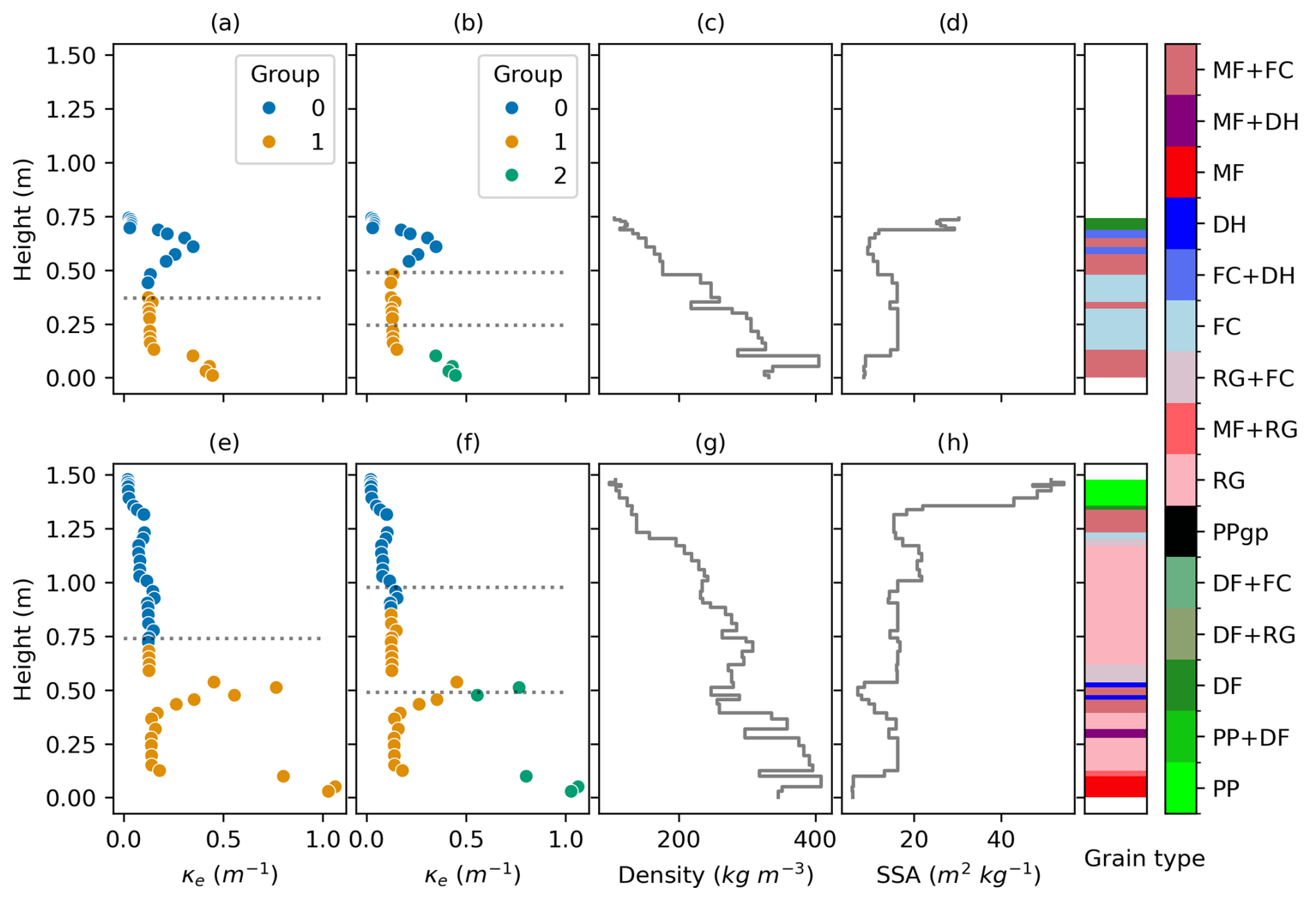
Figure 2 Snowpack properties (scattering, density, SSA, and grain type) from Crocus and SMRT simulations at WFJ for the winter of 2013–2014. The first row is 8 December 2013, and the second row is 9 February 2014. The grouping using the k-means clustering is shown by the colors in panels (a), (b), (e), and (f). The h_norm used for the equal-thickness grouping is also shown with the dashed lines. The colors and nomenclature for the grain types follow the international classification for seasonal snow on the ground (Fierz et al., 2009).

The grouping and averaging methods were first investigated at three different sites that represent alpine (WFJ), maritime (SAP), and arctic (TVC) snowpacks. Figure 3 shows the simulated backscatter with SMRT for the 2013–2014 winter season. For easier representation, only the grouping with three layers is shown here: 3-equal with the h-average method was worst in terms of reproducing the n-layer backscatter, 3-cluster with the h average improves the performance but still cannot consistently replicate the n-layer backscatter throughout the season, and 3-equal with a τ average achieved a similar performance to 3-cluster with the τ-average model but had issues early in the season for WFJ and SAP. Using the τ average was superior to the h average for preserving the backscatter. The backscatter of the arctic snowpack at TVC is well-represented for most grouping methods. Using the cluster method is not always better than equal grouping during the season. For some dates, the cluster is close to equal grouping (Fig. 2) and the resulting backscatter is similar.

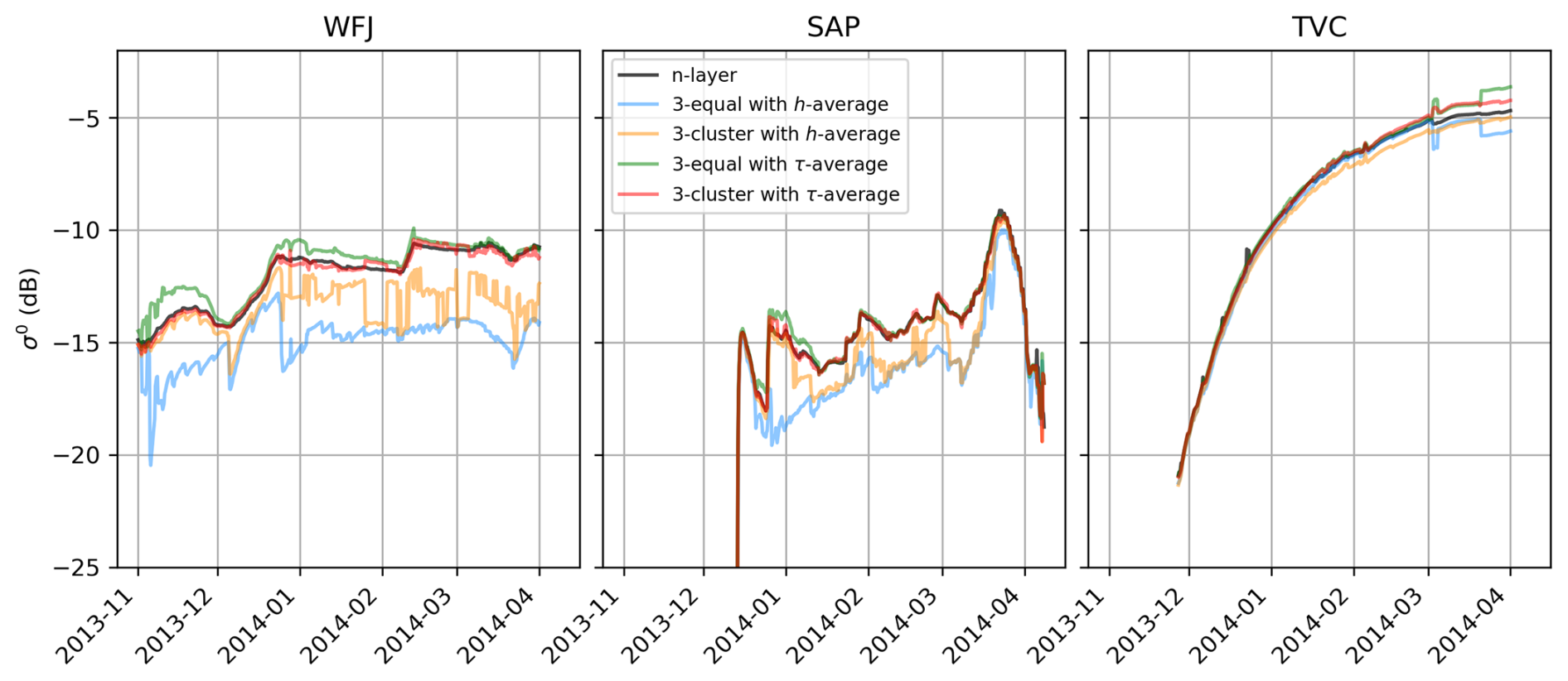
Figure 3 Backscatter time series for the reference simulations and different three-layer grouping and averaging methods. The simulations for the 2013–2014 season at WFJ, SAP, and TVC are shown.

To better understand the performance of the cluster approach, Fig. 4 shows biases for 3-equal and 3-cluster with the h-average method as a function of snow properties; 3-equal with the h-average method shows increased negative biases for low density and a high SSA at the WFJ and SAP sites compared to biases for the cluster method, which were smaller and constant across the density and SSA. These layers have less scattering and low SWE (high SSA and low density) than other snow layers, supporting the idea that these snow layers were better handled by the cluster grouping because of the ability to identify and group these transparent layers. Biases for both methods tend to increase as the snow layers are warmer. For TVC, biases remain relatively small (<1 dB) for the majority of the season because the SWE is fairly small (<100 mm), and changes in stratigraphy are less frequent due to the lack of precipitation. Arctic snowpacks also tend to have a simple stratigraphy well-represented by a two-layer snowpack (Vargel et al., 2020; Royer et al., 2021a).

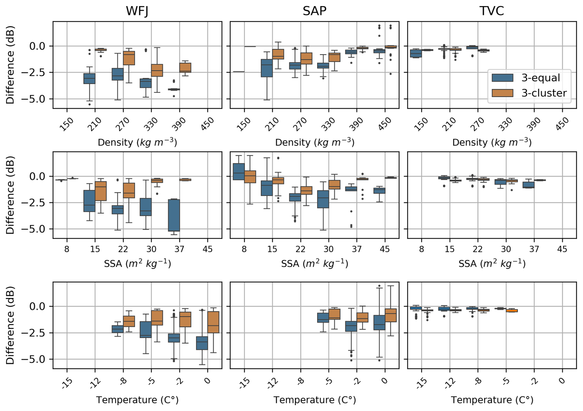
Figure 4 Boxplot of the difference in backscatter as a function of mean density, SSA, and temperature per simulation for the sites WFJ, SAP, and TVC for the 2013–2014 season.

Analysis of all sites and seasons (Table 2) produces results consistent with the example cases shown in Fig. 3. Not surprisingly, aggregating the layers into a one-layer snowpack with the h-average method resulted in the highest overall bias. Increasing the number of layers (from one to three) and using a cluster grouping resulted in a lower RMSE and a greater R² (Table 2). Again, 3-cluster with the τ-average method is the most promising method for preserving SWE and the scattering behavior because the RMSE for all of the sites is lowest (RMSE =0.5 dB and R²=0.98). TVC, KUT, and SWA had the highest RMSE (0.7–0.8 dB) compared to BYL, CDP, and UMQ, which had the lowest RMSE (0.3–0.4 dB). There is no pattern with respect to snow climate (alpine and arctic) and the performance of 3-cluster with the τ-average method; 2-cluster with the τ average and 3-equal with the τ average produced the second-best overall RMSE of 0.7 dB and R²=0.97, while 3-equal with the τ average achieved lesser but similar performance to 3-cluster with the τ-average model. This indicates that the cluster grouping is less important in terms of preserving the microwave behavior than the τ average of the snow properties.

Table 2 Overview of the RMSE and correlation coefficient (R²) of the estimated backscatter for the different grouping and averaging methods for all sites and all seasons. The column in bold shows the best-performing method.

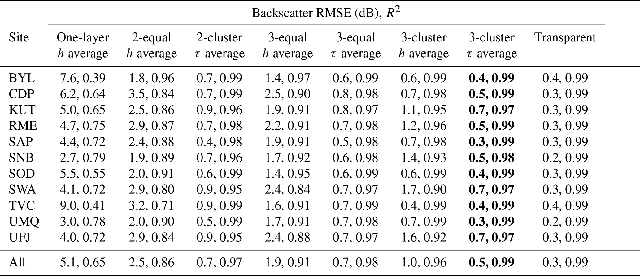
Averaging layers using the h average does not sufficiently reduce the backscatter RMSE below 1 dB. However, using the τ average brings the RMSE down to under 1 dB. The τ-average method was effective in preserving the backscatter because this averaging approach places more weight on strong scattering layers due to κ_e. The thickness is also a good indicator of scattering because a thicker layer will scatter more than a thin layer with the same scattering properties. This is an effective way of averaging snow properties and preserving the scattering behavior of the snowpack. The τ-average method seems the most promising method for preserving the scattering behavior.

Transparent layer simulations yielded on average an RMSE of 0.3 dB from full layering simulations (Table 2). This indicates that, on average, the internal layering contributions are around 0.3 dB based on the number of layers from SVS-2/Crocus simulations and the different sites and seasons. For the arctic sites (BYL, TVC, and UMQ), the RMSE values from 3-cluster with the τ-average method and the transparent experiment are the same, indicating that the snowpack reduction method almost perfectly preserves the scattering of the snowpack, with the exception of the layer contributions. For the other sites, especially the alpine sites (KUT, SWA, and UFJ), the RMSE of 0.7 dB for 3-cluster with the τ-average method is larger than the layering contribution, indicating that there are still some effects from the reduction method that are not accounted for.

The issue raised in Fig. 2 about mixed layers between groups can be discussed further with the results of the transparent layering. The two layers at 50 cm in Fig. 2f that were grouped with the layers at the bottom with three k-means do not affect the scattering effect of the snowpack since they will be accounted for in the τ average, whether they are in group 0 or group 1. However, attenuation of the scattering from these layers can differ if the layers are moved upward or downward in the snowpack. The other effect was the vertical change in permittivity that was modified, impacting the reflection of the signal in the internal layers. However, because the reflection of the internal layers was minimal (≈0.3 dB) and the change in backscatter was <1 dB for all of the sites, it was concluded that the overall effect of this special grouping case was minimal.

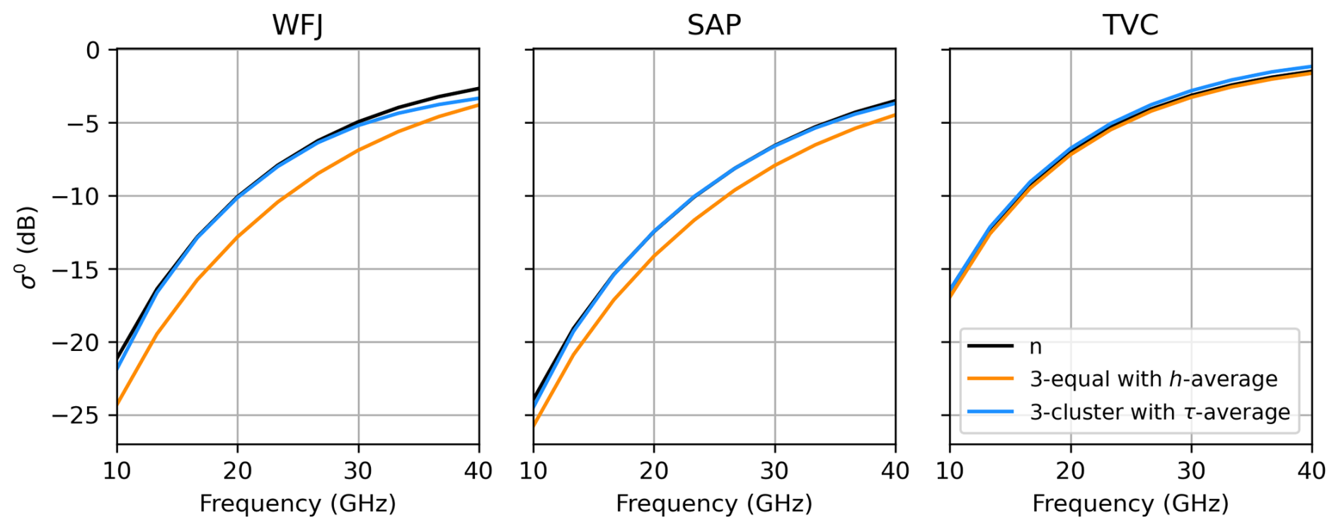
Figure 5 Backscatter simulations of 3-equal with the h-average and 3-cluster τ-average methods as a function of frequency.

The simulations were performed earlier at VV polarization since this will be the primary polarization of TSMM, but similar simulations were also done at HH polarization (not shown here) and yielded a higher RMSE of 0.1 dB than VV polarization.

3.2 Frequency dependence

An analysis of frequency dependence was conducted across the X-band to Ka-band range (10 to 40 GHz), encompassing regimes where volume scattering is significant. This interval includes the frequency utilized in the present study (17.25 GHz), which corresponds to the upper frequency selected for the Terrestrial Snow Mass Mission (Derksen et al., 2021). The errors between simulations with full layering and 3-cluster with the τ average were similar to the values reported in Table 2 from 10 to 30 GHz. The performance of 3-cluster with the τ-average method is based on κ_e, which is frequency-dependent. This allows us to obtain similar results when frequency (and sensitivity to volume scattering) increases. Although differences can be noted between sites, our method preserved similar performances from 10 to 30 GHz. At 10 GHz, a different simulation setup would be needed since the soil contribution will dominate. Above 40 GHz, 3-cluster with the τ-average method became similar to 3-equal with the h average because the backscatter came from the snow surface as the frequency increased and the penetration depth decreased.

3.3 Implications for SWE retrievals

In SWE retrieval applications, the number of variables that need to be optimized plays a crucial role in determining the accuracy and efficiency of the retrieval process. One of the most significant advantages of adopting a radar-equivalent snowpack representation is its ability to reduce the number of optimized variables without substantial loss of information. Now, an important choice still has to be made regarding whether two or three layers are best. We saw that backscatters from a two-layer snowpack are slightly degraded compared to using a three-layer snowpack (Table 2). Despite this small degradation when simplifying into two layers, retrieval applications could still benefit in terms of computational efficiency and reduced solution space, which can be advantageous for operational or large-scale applications. However, simplifying into three layers would offer a better representation of snowpacks across all climates.

In a Bayesian retrieval, calculating the mismatch term involves running a radiative transfer model and then optimizing the resulting posterior parameters. Using radar-equivalent snowpack would imply that the optimization is performed for a snowpack represented by a reduced number of layers rather than its full complexity. Concurrently, the prior distributions for snow properties, which are sourced from SVS-2, are also reduced to this number of layers. This consistent approach ensures that both the forward modeling for the mismatch term and the prior information are based on a comparable simplified structural representation of the snowpack.

4 Conclusions

In this paper, we showed the performance of our methods in simplifying complex multilayered snowpacks to three layers or less while preserving their microwave scattering behavior and bulk snow mass. We evaluated our method using simulated snow properties generated by the Crocus snowpack scheme at 11 sites, which were input into the SMRT model to calculate backscatter at 17.25 GHz and VV polarization. This emulates potential future measurements from the Canadian Terrestrial Snow Mass Mission. The method was a k-means clustering algorithm that grouped snow layers based on the extinction coefficient and the height of a layer in the snowpack. Then, a weighted average using the extinction coefficient and the thickness was applied to the snow properties, except for density, for which snow layer thickness was used as a weight to preserve SWE. We found that the averaging method was more important than the grouping method for preserving the backscatter. Reducing the original 50 snow layers to 3 layers using this method reproduced the snowpack backscatter of the original multilayered snowpacks with an overall RMSE of 0.5 dB and R²=0.98. Using this methodology in SWE retrieval algorithms allows snowpack simplification without nearly impacting the scattering behavior or compromising the geophysical properties. Reduction in the mathematical complexity of the SWE cost function and reduction in computation by up to 80 % (Appendix A1) can be gained by using fewer layers in SWE retrievals. We proposed radar-equivalent snowpack, a simple method that can also be applied to other fields of study that need to simplify a multilayered snowpack without compromising the electromagnetic properties of snow. The algorithm averages snow layers to obtain effective layers with snow properties that have an electromagnetic equivalent, so the potential application must be specific to the chosen frequency. This method could be adapted to passive microwave remote sensing where the signal is also highly dependent on snow scattering, including ice sheet or sea ice remote sensing where the microwave signal could be simplified to focus on radiation-relevant layers. For the TSMM workflow, this radar-equivalent snowpack allows for simplification of the modeled snowpack from SVS-2/Crocus and reduction of the number of unknowns in the SWE retrieval. It can also be used in assimilation schemes to reduce the computation time required to calculate a backscatter ensemble from a collection of snowpack members. For these reasons, this method offers an effective way of linking physical snow modeling and snow radiative transfer modeling in SWE retrievals.

Appendix A: Computation efficiency

Computation time was also estimated for each method to evaluate the gain in computational efficiency. The reduction in the computation time of the backscatter to reduce a complex multilayered snowpack (50 to 10 layers) to 2 or 3 layers is shown in Table A1. The largest reduction in computation time was from 50 layers to 2 layers at 87 %, and the smallest was from 10 to 3 layers at 39 %. Even the smallest reduction is considerable and motivates this work in the context of operational SWE retrieval implementations, where these computations have to be done at large scales.

Table A1 Computation time of backscatter with the SMRT and grouping methods. Results in various configurations of the number of layers are shown here. The grouping times for the k-means method are also shown. The backscatter computation time for three layers is 0.15 s, and for two layers it is 0.12 s. The grouping and averaging (3-cluster with a τ average) method takes 0.005 s.

Appendix B

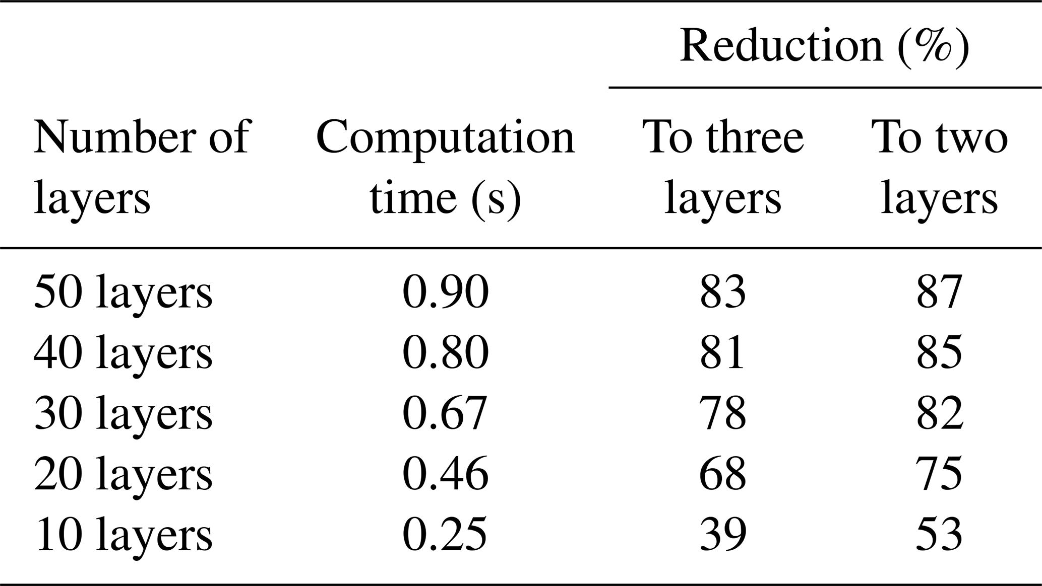
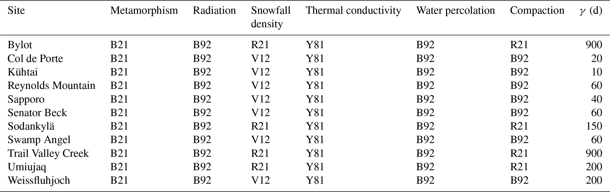
Table B1 Crocus schemes and parameters used at the different sites. The meaning of the Crocus schemes can be found in Lafaysse et al. (2017) and Woolley et al. (2024). The different options are defined in their respective papers – B21: modified C13 of Carmagnola et al. (2014); B92: Brun et al. (1992); R21: Royer et al. (2021b); V12: Vionnet et al. (2012); and Y81: Yen (1981). The γ parameter represents the snow aging coefficient and was determined at the sites in Gaillard et al. (2025), except for Reynolds Mountain, for which the default value of 60 d was used.