Meltwater from the Greenland ice sheet and its water isotope distribution in Dickson Fjord, East Greenland

Glacier retreat and mass loss in East Greenland have profound implications for global sea-level rise, making it crucial to understand the complex dynamics of glacier–ocean interactions. Currently, our knowledge of East Greenland glacial fjords is limited, and the processes occurring directly in front of these glaciers, particularly the fate of subglacial meltwater, remain poorly understood. In this study, conducted in Dickson Fjord, East Greenland, in August 2022, hydrographic and stable water isotope measurements at various depths and fjord locations were carried out, starting from the terminus of the marine-terminating glacier. Employing a drone-deployed ocean profiler, we obtained salinity and temperature profiles as close as 20 m from the glacier terminus. We found that the terminus is primarily in contact with a cold Polar Water layer, with temperatures ranging between −0.8 and −1.7 °C. Within this layer, we observed an increase in temperature close to the glacier terminus. In the surface water layer, we identified two distinct depleted water isotope signals originating from the glacier: one located at the surface and the other near the freshwater freezing line, separated by non-depleted water. Based on our findings, we hypothesise that subglacial meltwater undergoes freezing upon encountering the cold Polar Water at the terminus. The buoyant ice crystals (frazil) formed during this refreezing process would then ascend to the surface, where they encounter positive ocean temperatures and melt. This frazil ice crystal formation process would explain the temperature increase in the Polar Water layer (due to latent heat released during freezing) and the depleted water isotope signal around the freshwater freezing line.

1 Introduction

Climate change has triggered an accelerated mass loss from the Greenland ice sheet (GIS), substantially contributing to the rise in global sea levels and Arctic Ocean freshening (Velicogna, 2009; Straneo and Cenedese, 2015). A significant portion of GIS mass loss (88 %) can be attributed to melting at the front of marine-terminating glaciers (Mortensen et al., 2020). However, GIS mass loss remains poorly understood as most studies have focused mainly on marine-terminating glaciers in west and southeast Greenland. Glaciers in East Greenland are less studied, even though they are also experiencing notable ice loss through dynamic thinning (Arndt et al., 2015; Khan et al., 2014). Along with the increase in supraglacial melt, the interaction of the deeper warmer Atlantic Water mass with the glacier terminus has been found to increase subsurface melting (Straneo et al., 2012; Zhao, 2022; Holland et al., 2008), further contributing to GIS mass loss. However, the scarcity of measurements at the ice–ocean interface limits our understanding of the complex meltwater dynamics at the ice–ocean boundary (Mortensen et al., 2020; Straneo and Cenedese, 2015; Straneo et al., 2012; Zhao, 2022). While studies have been conducted in the water column in close proximity to Antarctic floating ice shelves (Fer et al., 2012; Stevens et al., 2014), comprehensive studies near the glacier terminus in East Greenland remain limited. Particularly, one of the main constraints for such studies derives from the life-threatening risk of sampling due to calving events (Holland et al., 2016).

Here, we present data from Dickson Fjord, East Greenland, at 72° N (Fig. 1). Dickson Fjord is part of the intricate Kempes fjord system, which includes Röhss Fjord and Rhedin Fjord. At Dickson Fjord's head lies the terminus of the Hisinger glacier, a marine-terminating glacier approximately 2.5 km wide and estimated to be around 150 m deep, serving as a major freshwater source into the fjord. The fate of the subglacial meltwater released at depth interacting with surrounding water is unknown. In this study we address the fate of glacial meltwater and the dynamics between glacier and fjord waters by using temperature and salinity measurements as close as 20 m to the terminus, along with in-fjord water isotope data. In addition, we identify and assess the mechanisms behind the observed temperature and salinity variations near the glacier terminus, assessing their implications for the thermohaline dynamics and meltwater distribution in Dickson Fjord. These findings contribute to ongoing efforts to accurately model and predict the impacts of glacial meltwater on the coastal region and its influence on ecosystem dynamics.

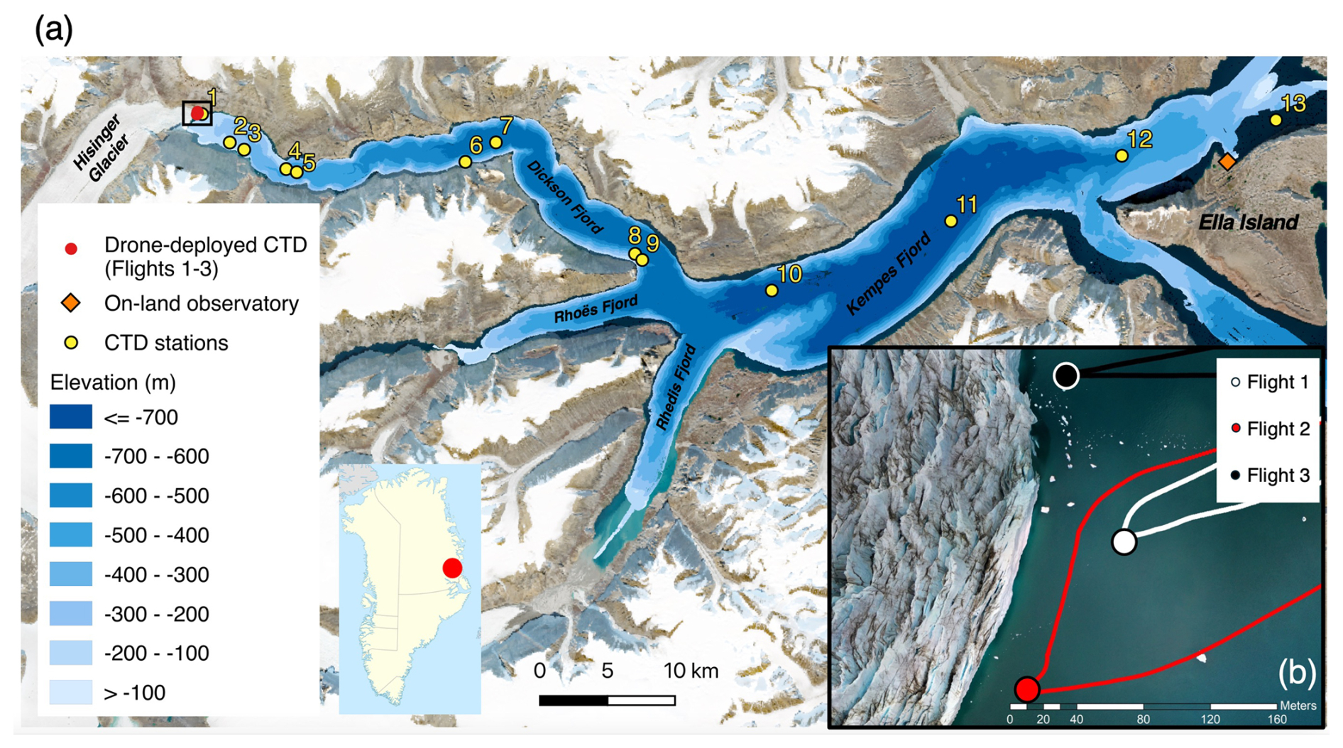
Figure 1 (a) Map of locations of measurement stations used in this study, including high-resolution bathymetry represented as a colour gradient. The green dots indicate the locations where the CTD was deployed. At stations 1, 5, 7, 9 and 13, water samples were collected for stable isotope analysis alongside the CTD deployment. The map was generated using Modified Copernicus Sentinel data August 2022/Sentinel Hub. (b) A close-up image of the flight trajectories of the drone-deployed CTD, courtesy of Jeffrey Taylor Kerby.

2 Theory and method

2.1 CTD data

To investigate the spatial variability in temperature and salinity in the fjord, we collected vertical CTD (RBRconcerto) profiles at various locations within Dickson Fjord up to Ella Island (Fig. 1a). To conduct measurements close to the glacier terminus, CTD measurements were done using a drone-deployed SonTek CastAway CTD (Poulsen et al., 2022). This allowed for three CTD casts to reach distances of around 20, 30 and 50 m from the glacier terminus (Fig. 1b). Due to constraints of the drone-deployed CTD, these casts do not exceed 100 m depth. For convenience, the stations have been numbered, with a distinction made between measurements conducted using the drone-deployed CTD (labelled flights 1–3) and the boat-deployed CTDs (stations 1–12) (Fig. 1a). The station number increases with the distance from the glacier. The measurements at stations 10 to 12 were conducted on 31 July; stations 2, 4, 6 and 8 on 2 August; stations 1, 3, 5, 7 and 9 and the drone-deployed casts on 14 August; and station 13 on 15 August.

The Practical Salinity Scale 1978 (PSS-78) was used to compute salinity and depth from the pressure, in situ temperature and conductivity measured by the CTDs. For calculation of the conservative temperature (temperature insensitive to pressure) and the specific heat capacity, used for calculations, the Python implementation of the Gibbs SeaWater (GSW) Oceanographic Toolbox of TEOS-10 package (The TEOS-10 Contributors, 2021) was used. Hydrographic sections of temperature, salinity and stable water isotopes were generated by linearly interpolating the data, with a resolution of 176 m along the horizontal distance and 0.6 m along the vertical depth. Scientific colour maps roma, romaO and hawaii (Crameri, 2023) have been used to prevent visual distortion of the data and to ensure accessibility for readers with colour vision deficiencies (Crameri et al., 2020).

2.2 Stable water isotope data

We collected stable water isotope samples from the water column to assess the presence and influence of glacier water, Polar Water and Atlantic Water. Samples were taken at five locations along the fjord, spanning 500 m near the glacier terminus to Ella Island, and at depths of 1, 5, 10, 20, 30, 50, 75, 100 and 150 m. At stations 1 and 13, additional samples were taken at depths of 200, 210, 220 (station 13) and 250 m (station 1). The samples were transferred to 2 mL glass vials and remained at room temperature until analysis. The stable hydrogen and oxygen isotope concentrations were determined using a cavity ring-down spectrometer, L2130-i Isotopic sH20 (Picarro Inc., USA).

To standardise the stable water isotope data measurements, the δ¹⁸O and δ²H values are expressed relative to the Vienna Standard Mean Ocean Water (VSMOW) as

$$\begin{array}{}\text{(1)}& {\displaystyle }\begin{array}{rl}{\mathit{\delta }}^{\mathrm{18}}\mathrm{O}\left(\mathrm{‰}\right)& =\left[{\displaystyle \frac{({}^{\mathrm{18}}\mathrm{O}{/}^{\mathrm{16}}\mathrm{O}{)}_{\mathrm{sample}}-({}^{\mathrm{18}}\mathrm{O}{/}^{\mathrm{16}}\mathrm{O}{)}_{\mathrm{VSMOW}}}{({}^{\mathrm{18}}\mathrm{O}{/}^{\mathrm{16}}\mathrm{O}{)}_{\mathrm{VSMOW}}}}\right]\\ & \cdot \mathrm{1000}\mathrm{‰},\end{array}\text{(2)}& {\displaystyle }\begin{array}{rl}{\mathit{\delta }}^{\mathrm{2}}\mathrm{H}\left(\mathrm{‰}\right)& =\left[{\displaystyle \frac{({}^{\mathrm{2}}\mathrm{H}{/}^{\mathrm{1}}\mathrm{H}{)}_{\mathrm{sample}}-({}^{\mathrm{2}}\mathrm{H}{/}^{\mathrm{1}}\mathrm{H}{)}_{\mathrm{VSMOW}}}{({}^{\mathrm{2}}\mathrm{H}{/}^{\mathrm{1}}\mathrm{H}{)}_{\mathrm{VSMOW}}}}\right]\\ & \cdot \mathrm{1000}\mathrm{‰}.\end{array}\end{array}$$

In Greenland, the δ¹⁸O value in glacial water has been measured to be −27.2 ± 0.2 ‰ (Rysgaard et al., 2024). To trace the origin of the ocean waters from the isotopic composition, the δ¹⁸O values can be plotted against the δ²H values. In the resulting diagram, samples of rainwater align along a straight line known as the meteoric water line (MWL), exhibiting a slope of about 8. These line equations are typically of the form ${\mathit{\delta }}^{\mathrm{2}}\mathrm{H}=\pm \mathrm{8}\cdot {\mathit{\delta }}^{\mathrm{18}}\mathrm{O}+\mathrm{d}$, where the constant term d is termed the deuterium excess and differs per region (Souchez et al., 2002). Interestingly, melting and refreezing have been found to decrease the slope of the δ²H–δ¹⁸O line, though the effect has no uniform effect on the d-excess value (Zhou et al., 2014). Given that the river water isotopic composition typically correlates well with precipitation composition, the river water isotope values are used to obtain local meteoric water lines (Zhou et al., 2014). In this study, isotope values will be compared to the Arctic Meteoric Water Line (AMWL), the Global Meteoric Water Line (GMWL), the Lena Meteoric Water Line (LMWL) and the Greenland ice sheet (GIS). The δ¹⁸O to δ²H line equations for the AMWL, LMWL and GMWL are taken from Willcox et al. (2023) and the GIS line equation from Rysgaard et al. (2024).

2.3 Atmospheric data

An on-land observatory on the north side of Ella Island (Ella Ø) measures atmospheric conditions, including air and skin temperature, relative humidity, and incoming radiation (Rysgaard et al., 2022). These data were used in heat budget calculations together with measurements of latent and sensible heat fluxes from an observatory in Zackenberg, East Greenland (74° N), to better understand the energy dynamics in the fjord (Sect. 3.5). Since quantities relevant for the latent and sensible heat fluxes, such as wind speed, relative humidity and temperature, are very similar between Zackenberg and the Ella Island observatories in August 2022, the average latent and sensible heat fluxes measured in Zackenberg during that period were used for the atmospheric heat estimate (Rysgaard et al., 2022). Important to note is that these values are not an exact representation of the actual latent and sensible heat fluxes, since they were not measured right above the water.

2.4 Water mass partition

To determine the water composition, water mass partitioning can be applied based on different water characteristics. Salinity, temperature, δ¹⁸O and δ²H are all characteristics that are specific to the different water types and can thus be used for water type identification. In a model brought forward by Washam et al. (2019), adapted by Mortensen et al. (2020), the subglacial freshwater and glacial ice melt partitions are calculated using both the observed salinity and temperature. Since this model assumes closed conditions, with only ice melting and freshwater inflow affecting water salinity and temperature, the model is not applicable in cases where external processes influence water temperature and salinity. To study whether the temperature increase closer to the terminus is caused by external circumstances or by warm subsurface meltwater mixing, the water masses were separately partitioned based on salinity, temperature and isotopic composition (δ¹⁸O). If the partition of meltwater computed based on the temperature does not correspond to the partition based on the salinity, this heat can not come from warm subsurface freshwater release and thus must come from external processes.

The following simple temperature-based partition formula has been used to compute the meltwater partition in the water body:

$$\begin{array}{}\text{(3)}& f_{\mathrm{T}}={\displaystyle \frac{T_{\mathrm{obs}}-T_{\mathrm{WT}}}{T_{\mathrm{MW}}-T_{\mathrm{WT}}}},\end{array}$$

where f_T represents the temperature-based meltwater fraction, T_obs the observed temperature, T_WT the temperature of the water type at that depth and T_MW the meltwater temperature. The same equation has been used for the partitioning based on water salinity and δ¹⁸O.

The meltwater temperature and salinity values were taken to be 0 °C and 0 PSU, respectively. Since the δ¹⁸O values of Polar Water are not depth-dependent, the measured values in the Kong Oscar fjord system for Polar Water (−1.1 ‰) and glacial meltwater (−27.2 ‰) are used (Rysgaard et al., 2024). For the δ¹⁸O-based water partitioning calculation, the surface waters were included, as these are going to be used to estimate the ratio of the different meltwater sources. Important to note is that the amount of surface water is likely underestimated due to sea ice formation resulting in a less depleted signal compared to the meltwater from which it is formed.

3 Results and discussion

3.1 Temperature and salinity

The temperature–depth and salinity–depth profiles for different stations along the fjord are shown in Fig. 2. To improve clarity, the plots in Fig. 2 include selected stations chosen based on their significance, showing noteworthy changes or unique characteristics. These profiles show the three distinct water layers typical of East Greenland glacial fjords: the surface water layer (0–20 m depth), the underlying Polar Water layer (20–120 m depth), and the Atlantic Water layer below (Straneo and Cenedese, 2015; Rysgaard et al., 2024). The surface layer is marked by low salinity values due to the freshwater dilution and high temperature caused by atmospheric warming, thus being the lightest layer and stably stratified. The underlying Polar Water layer has low temperatures below the freshwater freezing point, ranging from −0.8 to −1.7 °C, and salinity values between 31.8 and 32.1 PSU, decreasing in temperature and increasing in salinity with distance from the glacier terminus. The bottom Atlantic Water layer has a relatively stable temperature along the transect, measuring at 0.7 °C at the largest depth measured (300 m), along with characteristically high salinity values measuring at 34.6 PSU at its deepest point, corresponding to Eurasian Basin Atlantic Water (Willcox et al., 2023).

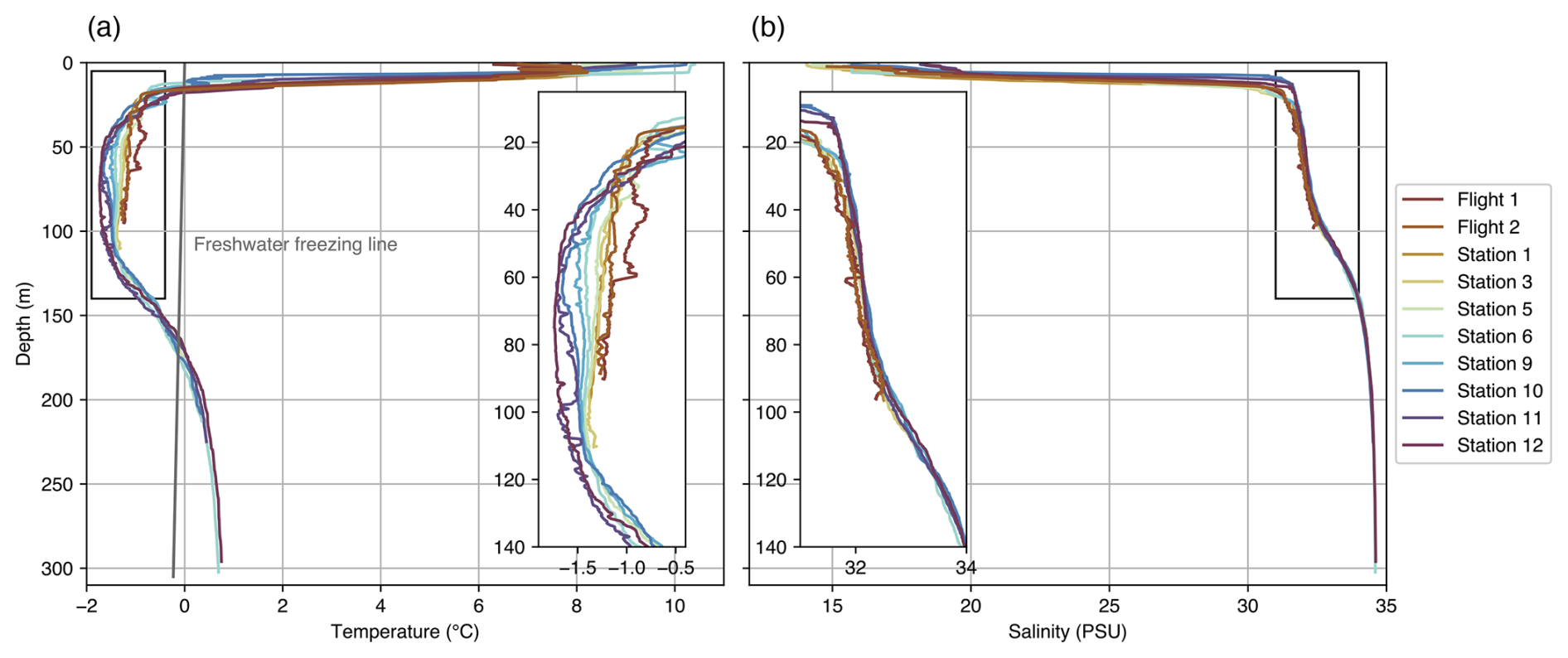
Figure 2 Temperature (a) and salinity (b) variations with depth measured at selected stations across the fjord. Zoomed-in sections are added between 5 and 135 m depth in both plots. In the temperature-depth plot, a pressure-dependent freshwater freezing line is added.

Since subsurface melt occurs when ambient seawater is above the pressure–salinity-dependent freezing point, the warm surface waters above the pressure-dependent freezing line (0 to 15 m) and deep Atlantic Water (from 170 m) could cause subsurface melting (Fried et al., 2018). Based on the bathymetric data shown in Fig. 1a, which indicate that the fjord terminus does not extend beyond approximately 150 m in depth – thereby limiting its interaction with Atlantic Water – we hypothesise that the primary subsurface melting occurs at the warmer surface water layer, in the upper 20 m.

The temperature–salinity (θ–S) structure (Fig. 3) reveals the key water types in Dickson Fjord, illustrating the presence and mixing of surface water, Polar Water and Atlantic Water layers. To more easily identify the spatial changes in the water types, grouping was applied based on the measuring location with respect to the terminus (Fig. 3a). Distinctions were made between the drone-deployed measurements, the deeper measurements relatively close to the glacier terminus (stations 1 and 2), in-fjord measurements up to station 9 and finally the out-fjord measurements up to Ella Island.

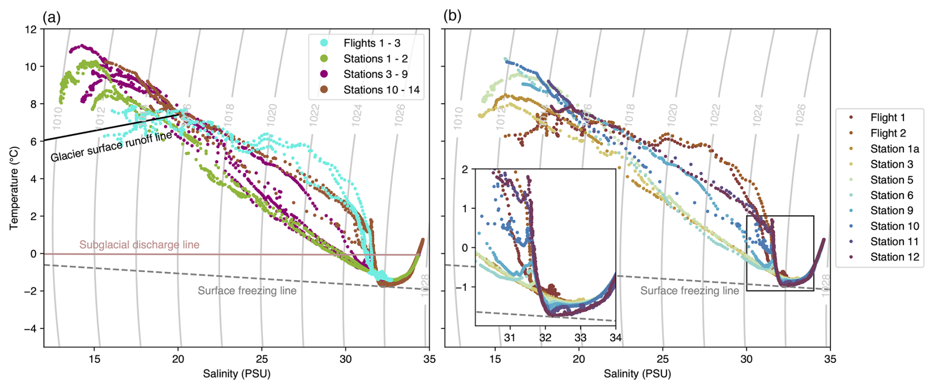
Figure 3 Temperature–salinity values of the profiles measured at all the stations grouped (a) and selected stations (b). Both plots include density lines (kg m⁻³) and the surface freezing line. The cluster plot includes a glacier surface runoff line connecting the surface waters with the glacial surface runoff and a subglacial discharge line connecting deep waters with subglacial discharge.

The θ–S values are relatively variable at salinities of around 31–32 PSU in Fig. 3. Figure 2 shows that this is due to relatively stable Polar Water layer salinity, whilst the temperature changes significantly. Additionally, Fig. 3c again clearly shows the Polar Water becoming colder at a distance further away from the glacier terminus, with the minimum temperature values (−1.74 °C) measured at station 12 at a salinity of 32 PSU nearly reaching the surface water freezing line values. Interestingly, the drone-deployed CTD measurements from flights 1–3 show lower temperatures at salinities below 18 PSU than the measurements conducted further away from the glacier terminus. The temperature of the flight measurements remains relatively constant, though fluctuating slightly between 6 and 7 °C, as salinity increases up to 26 PSU. This pattern contrasts with nearby stations 1 and 2, where warmer and fresher water cools from 8 to 2 °C as salinity increases in this range.

A glacier surface runoff line is plotted in Fig. 3a to investigate supraglacial runoff mixing (Mortensen et al., 2020). Thermal satellite data showed that these glacier surface waters are released with a temperature of approximately 4 °C (Fig. A1, Appendix A). As glacier surface runoff has a salinity of 0 PSU, the slope between these values would be a line connecting the surface waters with the point (θ, S) = (4 °C, 0 PSU). Interestingly, a slope change occurs in the lower-salinity waters (15–17 PSU), with the lowest-salinity water slope parallel to, or even steeper than, the glacier surface runoff line (Fig. 3a). This phenomenon, indicating freshwater input at the surface, appears up until station 5. To investigate the presence of subglacial discharge in the deeper water body layers, a subglacial discharge line was plotted. This represents the line connecting the deeper water body at approximately the depth corresponding to the draft of the tidewater glacier and the subglacial discharge water (Mortensen et al., 2020). Since subglacial discharge is freshwater at its melting temperature, this water type is characterised by the point (θ, S) = (0 °C, 0 PSU). The points do not fall along the subglacial discharge line, indicating no subglacial discharge plume is present.

To examine the spatial temperature and salinity patterns in more detail, temperature and salinity sections were generated (Fig. 4). Interestingly, there is little variation in the Polar Water (PW) and Atlantic Water (AW) layers between the profiles measured on 2 August (light purple) and 14 August (dark purple), as shown in Fig. 4b, c, e and f. As expected, there is a larger variation in the surface water layer, as evident from the 9 °C contour in Fig. 4a and the 17 PSU contour in Fig. 4d.

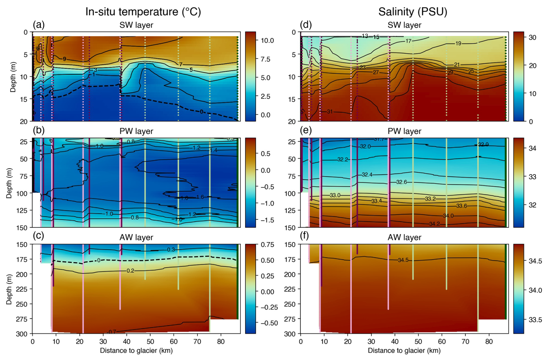
Figure 4 In situ temperature and practical salinity sections in the SW, PW and AW layers extending from 20 m to 87 km from the glacier terminus. The dotted light green, light purple, dark purple and dark green lines represent profiles measured on 31 July and 2, 14 and 15 August 2022, respectively. Contour lines have been added for every 2 units in the SW layers, for every 0.2 units in the PW layer and for every 0.5 units in the AW layer.

3.2 Stable water isotopes

To investigate further details in the spatial variation in the stable isotopes, along-fjord sections are shown in Fig. 5, along with a plot of δ¹⁸O vs. δ²H to trace the water origin. The δ¹⁸O and δ²H sections illustrate three distinct depleted water signal layers, as highlighted by the contours plotted in the δ¹⁸O section. The first of these is a shallow surface water layer, which can be distinguished in Fig. 5a by the contour values below −4 ‰ at depths less than 5 m. This depleted signal extends from the glacier terminus to approximately 35 km from the terminus. Below this surface layer, a second depleted signal is observed, extending from the terminus to 87 km, with the depletion decreasing with distance from the glacier. Notably, there is a sharp separation between these two signals at the 5 m depth, as marked by the −2 ‰ contour in Fig. 5a, where the values become less depleted. The third depleted signal, though less prominent than the surface signals, is found in the Polar Water layer at depths between 50 and 80 m, extending from the terminus to 87 km. Interestingly, this deeper signal becomes slightly more depleted further from the terminus, as marked by the −2 contour in Fig. 5a. In the δ¹⁸O vs. δ²H plot in Fig. 5c, the dataset values fall between the Arctic Meteoric Water Line (AMWL) and the Lena Meteoric Water Line (LMWL). Similarly to the meteoric water lines, the fitted line slope appears to be around 8, with a deuterium excess value (d) of 2.18.

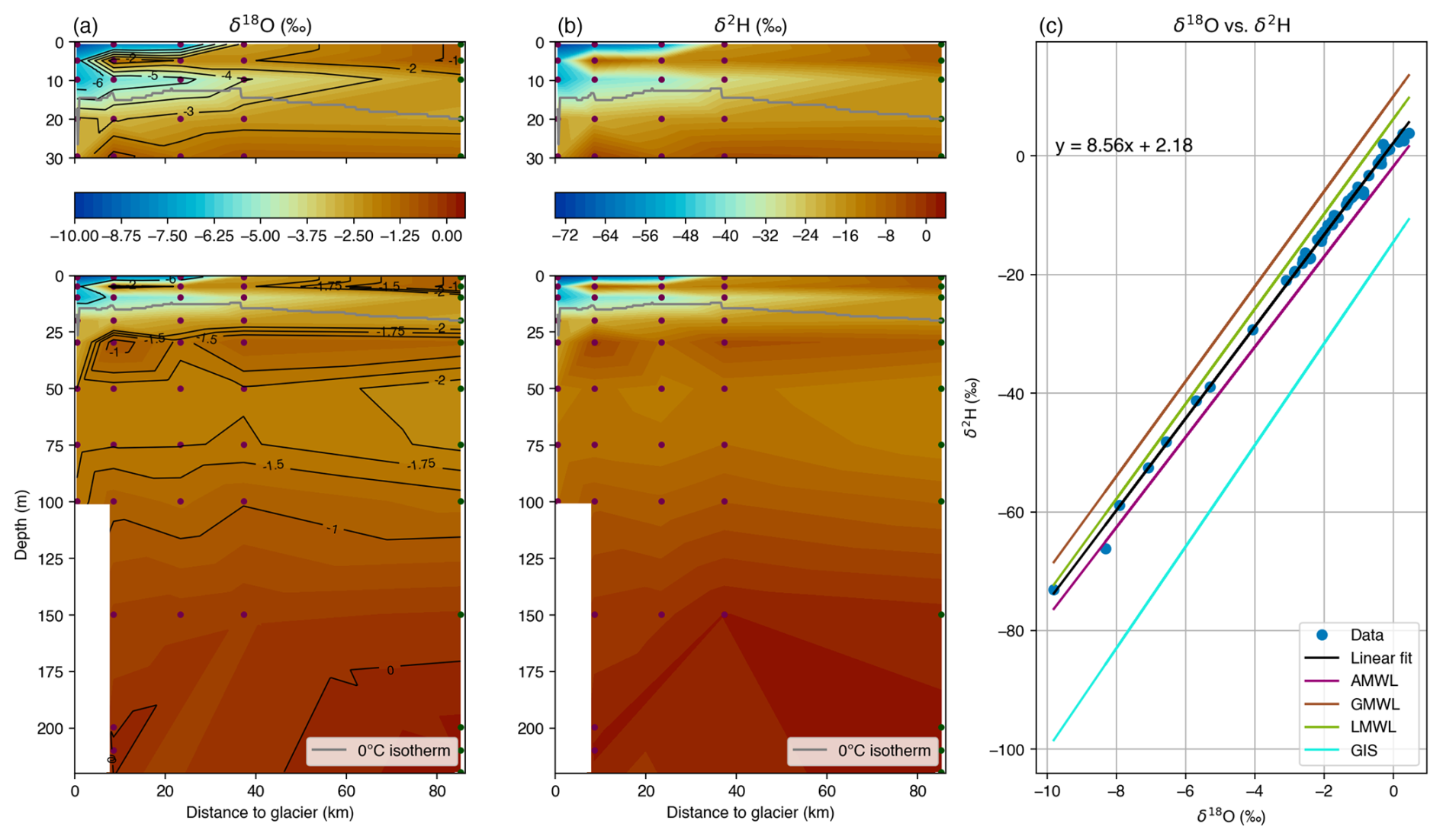
Figure 5 Sections of δ¹⁸O (a) and δ²H (b) extending from 0.5 to 87 km from the glacier terminus and a plot with the δ¹⁸O values plotted against the δ²H values (c). All the values are represented in units of per mille (‰). In (a) and (b), the dark purple and dark green dots represent the measurement data collected on 14 and 15 August, respectively. Additionally, a 0 °C isotherm is plotted to highlight the freshwater freezing point. Contours with varying intervals have been added to (a). In the rightmost plot, a solid black line represents the linear fit of the data points, plotted alongside the AMWL, the GMWL, the LMWL (Willcox et al., 2023) and the GIS line (Rysgaard et al., 2024).

The upper depleted signal, down to 5 m depth up to approximately 35 km from the glacier, is coupled with low salinity, which is typical of glacial meltwater. This upper surface meltwater signal likely results from glacial surface runoff, ice mélange and subsurface melting. The second depleted signal at around 10 m depth could be attributed to subsurface melting caused by positive ocean temperatures in contact with the terminus (e.g. Fried et al., 2018) or by melting frazil ice formed from the refreezing of subglacial discharge, or a combination of both. The frazil ice crystal processes will be explained in more detail in Sect. 3.4. Although, for most of the width, the terminus is too shallow to come into contact with the warmer Atlantic Water to cause surface melt at depth, there is still a slightly depleted water signal distinguishable in the Polar Water layer. This signal may result from Polar Water transported into the fjord, which has been measured to have δ¹⁸O values of around −2 ‰ at Kangerdlugssuaq Fjord, East Greenland (Azetsu-Scott and Tan, 1997), or it could originate from mixing within the fjord system.

In Fig. 5c the fitted line lies between the AMWL and the LMWL. A decrease in d-excess value could be attributed to contributions from the GIS, since the d-excess for the GIS line is much smaller compared to the relevant meteoric water lines shown. An interesting observation from the isotopic analysis of Rysgaard et al. (2024) is that measurements taken in the out-fjord region of East Greenland exhibit a closer alignment with the LMWL. This suggests a more substantial contribution from the Greenland ice sheet closer to the glacier. Further, the slope of the fitted line seems to be slightly less steep compared to the meteoric water lines, which could be the result of meltwater contribution to the water body, as described in Sect. 2.2.1. We compared our measurements to those by Azetsu-Scott and Tan (1997), who studied two sites in Kangerdlugssuaq Fjord: one near the terminus of an active tidewater glacier and another at the fjord's head. Their study showed a gradual increase in δ¹⁸O values with distance from the terminus, ranging from −15.0 ‰ near the glacier to −3.8 ‰ at the fjord's mouth at depths of 0 and 5 m. Similar to our results, they found lower (more negative) δ¹⁸O values at the surface compared to measurements at 5 m depth. Their measurements also show a difference in δ¹⁸O values at 0 and 5 m depth that persisted for approximately 50 km from the terminus. Beyond this point, the δ¹⁸O values are the same between 0 and 5 m, which we also see in Fig. 5a, showing the variability in glacial surface meltwater near the terminus.

Glacial meltwater sources can be identified by integrating δ¹⁸O isotopic data with temperature and salinity data (Hennig et al., 2024). Notably, the surface water measured beyond 35 km from the terminus, outside Dickson Fjord, is fresh (17–21 PSU; Fig. 4d) but not isotopically depleted (between −1 ‰ and −2 ‰; Fig. 5a). This surface freshwater may originate from seasonal ice melt (Solomon et al., 2021). During the freezing process, heavier isotopes are preferentially incorporated into the ice (fractionation factor of +1.6 ‰–2.3 ‰), resulting in sea ice meltwater being less isotopically depleted compared to the original seawater (Alkire et al., 2015).

To investigate the presence of sea ice meltwater, the salinity–δ¹⁸O relationship is shown in Fig. 6a. The lack of a clear linear correlation between salinity and δ¹⁸O suggests the influence of sea ice meltwater, particularly in the points with low salinity and low δ¹⁸O values in the top left of Fig. 6a (Azetsu-Scott and Tan, 1997). Station 1 is the only station showing some correlation between salinity and δ¹⁸O. A linear fit for station 1 gives a δ¹⁸O value of −14.5 ‰ at zero salinity, which is higher (less negative) than the measured δ¹⁸O for glacial meltwater (−27.2 ‰; Rysgaard et al., 2024). It is also higher than the values measured by Azetsu-Scott and Tan (1997), who found δ¹⁸O values at 0 salinity of −24.2 ‰ at the head of Kangerdlugssuaq fjord and −19.0 ‰ in the outer fjord. This higher value may be because the data point at 5 m depth shows a δ¹⁸O value that is higher than expected for its salinity (Fig. 6a). Additionally, Fig. 6b shows the temperature–salinity diagram with isotope colours, where the three freshest data points (<15 PSU) are the most depleted. The six low-salinity, less depleted δ¹⁸O points from Fig. 6a are clearly distinguishable within the range of 15–20.5 PSU and 7–10 °C. Along with these less depleted δ¹⁸O values, the salinity range 15–30 PSU shows a variability in isotope values, showing the presence of both glacier meltwater and PW in this layer.

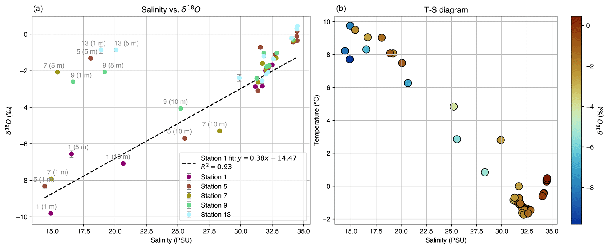
Figure 6 (a) The relationship between salinity and δ¹⁸O, with data points colour-coded based on station and labels indicating station numbers and depths for points with salinity below 29. A dashed black line indicates the linear fit for station 1, with the corresponding equation and R² value shown in the legend. (b) Temperature–salinity diagram with δ¹⁸O indicated with a colour gradient.

3.3 Water mass partitioning

Figure 7 presents the meltwater partition sections based on water type salinity, temperature and δ¹⁸O. The sections reveal a significant discrepancy between the temperature-based and salinity-based partition values, with the temperature-based values being significantly larger. This discrepancy confirms that the higher temperature close to the terminus in the Polar Water body does not originate from warmer liquid glacial meltwater.

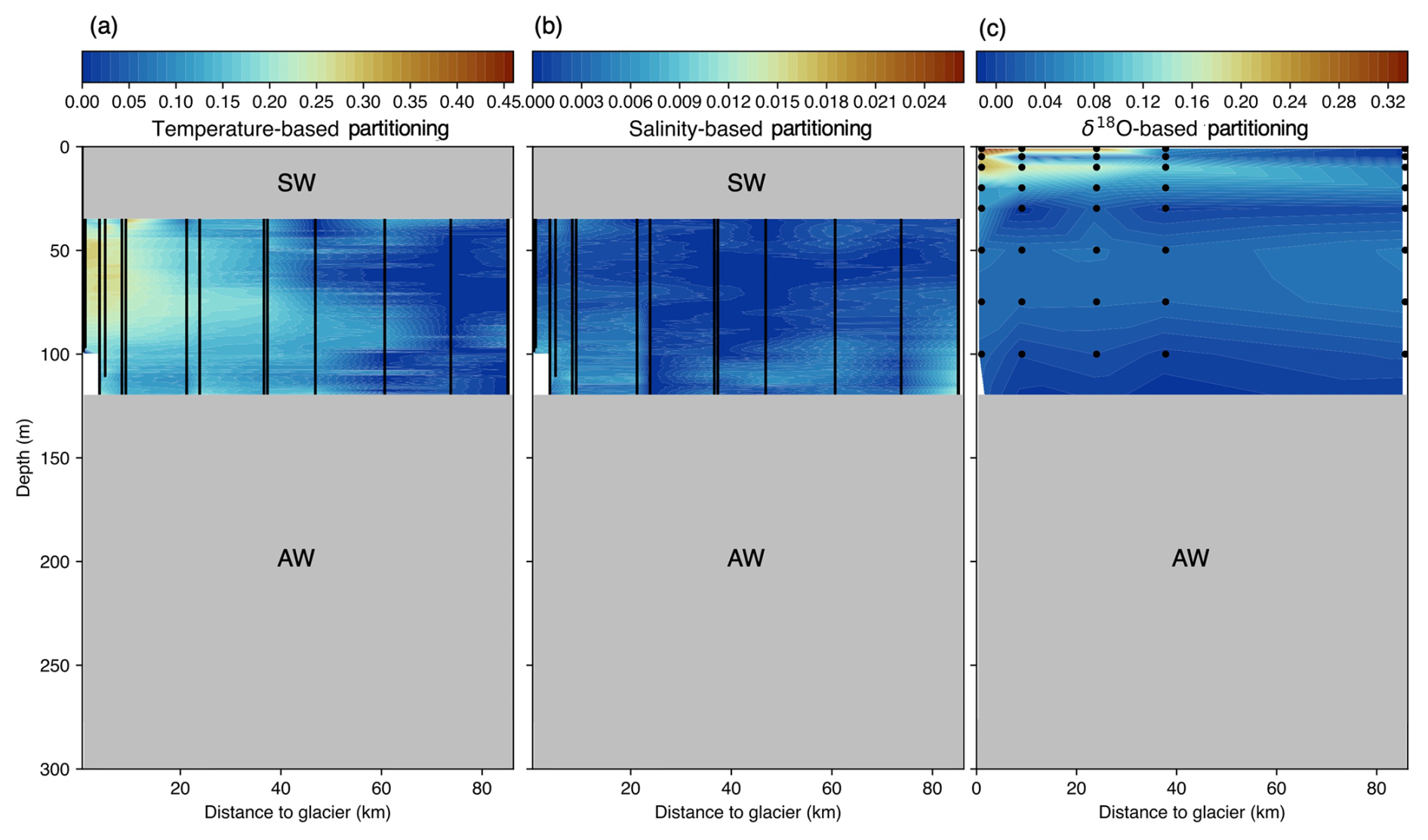
Figure 7 Graph depicting the Polar Water layer meltwater partition based on water temperature (a), salinity (b) and δ¹⁸O (c). The black dots represent the data points. The surface water (SW) and Atlantic Water (AW) layers are not considered in the temperature- and salinity-based partitioning calculation and are thus covered by grey blocks. In the δ¹⁸O partitioning, only Atlantic Water has been excluded from the partitioning.

Using the salinity-based meltwater partition values, the corresponding freshwater contribution to the temperature in the water body was computed. This contribution was then subtracted from the observed temperature section to calculate the excess heat required to reach the measured temperatures. This heat was obtained through element-wise multiplication of the excess temperature matrix with the specific heat capacity and density matrices. After applying a 2D Riemann sum to the resulting matrix and multiplying this value by the estimated average fjord width, 3 km, an excess Polar Water layer heat estimate of 1.1 ×10¹⁶ J was found in Dickson Fjord (up to station 9). The discrepancy between the Polar Water layer salinity-based and δ¹⁸O-based partitioning can be explained by the salinity values being compared to the minimum value at each depth rather than an absolute value since the salinity can also be changed by freshwater sources that are not subglacial meltwater. Thus, these values are taking the mixing and transition of the various water bodies into account, whereas with the δ¹⁸O-based partitioning this was not necessary. The only contribution to the δ¹⁸O depletion is glacial meltwater, freezing processes and precipitation, making it safe to assume a constant δ¹⁸O Polar Water value along the different depths but having a higher partitioning of meltwater in the Polar Water layer as a result (since the spatial variance of salinity and δ¹⁸O in only the Polar Water layer is not as high, comparatively).

Since the Dickson Fjord width remains relatively constant, the δ¹⁸O section can be used to roughly estimate the meltwater ratio in the fjord. The ratio of surface meltwater (SMW), subsurface meltwater (SSMW) and Polar Water layer meltwater (PLMW) was estimated to be $\mathrm{22}\mathit{\%}:\mathrm{31}\mathit{\%}:\mathrm{47}\mathit{\%}$. However, the surface meltwater partition is underestimated because the effect of sea ice formation, which decreases δ¹⁸O depletion, was not accounted for in the calculations.

3.4 Frazil ice crystal formation

Bathymetry measurements show that the terminus is exclusively in contact with the surface waters and cold Polar Water. Since the seawater temperatures in the Polar Water layer are below freshwater freezing temperature (Fig. 2a), we hypothesise that the meltwater refreezes once it is released at depth. Frazil ice crystals are then formed because of this freezing process, releasing latent heat to the ambient water. These ice crystals then slowly float to the surface due to their buoyancy (Dmitrenko et al., 2010), melting once they reach freshwater melting temperatures at the surface, releasing freshwater into the fjord. A schematic of this process is displayed in Fig. 8. A similar refreezing effect was observed by Marchenko et al. (2017) near the glacier terminus of Paula Glacier in Spitsbergen. In that paper, the authors also attribute the refreezing to meltwater mixing with seawater below the freshwater freezing point, leading to the formation of frazil ice crystals. A comparable process of frazil–platelet ice crystal formation has been described by Hoppmann et al. (2020), with a difference being that in our case, the primary freshwater source is surface freshwater released at depth rather than basal melt. This process could explain the excess heat in the Polar Water layer, as this may result from latent heat released by meltwater refreezing at depth. Additionally, the melting of ice crystals in the surface water layer would explain the freshwater input observed in the surface waters away from the terminus (up to station 5) in Fig. 3a. Assuming a stagnant water body, for the frazil ice crystal formation to account for the excess heat estimate in the Polar Water layer, the total volume of meltwater to be refrozen equals 3.4 ×10⁷ m³. Along with the excess heat, this refreezing process would also clarify the second surface depleted δ¹⁸O signal in Fig. 5a (indicated by the −4 ‰ contour), which indeed occurs around the freshwater freezing line, where the ice crystals would melt and the glacial freshwater be released. Since the Polar Water layer is likely more stagnant than the surface layer, this latent heat could build up over time. When this accumulated heat is then transported out of the fjord due to a net outward PW layer current, it may explain the observed heat increase up to 40 km from the terminus. Comparing the refreeze volume to the meltwater release estimates by Karlsson et al. (2023) this value seems to be close to the surface meltwater estimate of 3.6 ×10⁷ m³ in August 2022. However, while this hypothesis aligns with the low Polar Water temperatures and could explain the excess heat observed in the isotopic sections, more research is required to validate the presence of frazil ice crystals in the Polar Water body. In situ observation of these crystals is crucial for this validation, although obtaining these observations is challenging (Hoppmann et al., 2020). We successfully captured images of these crystals in the Polar Water body near the glacier terminus. This aspect of our work will be detailed and published elsewhere.

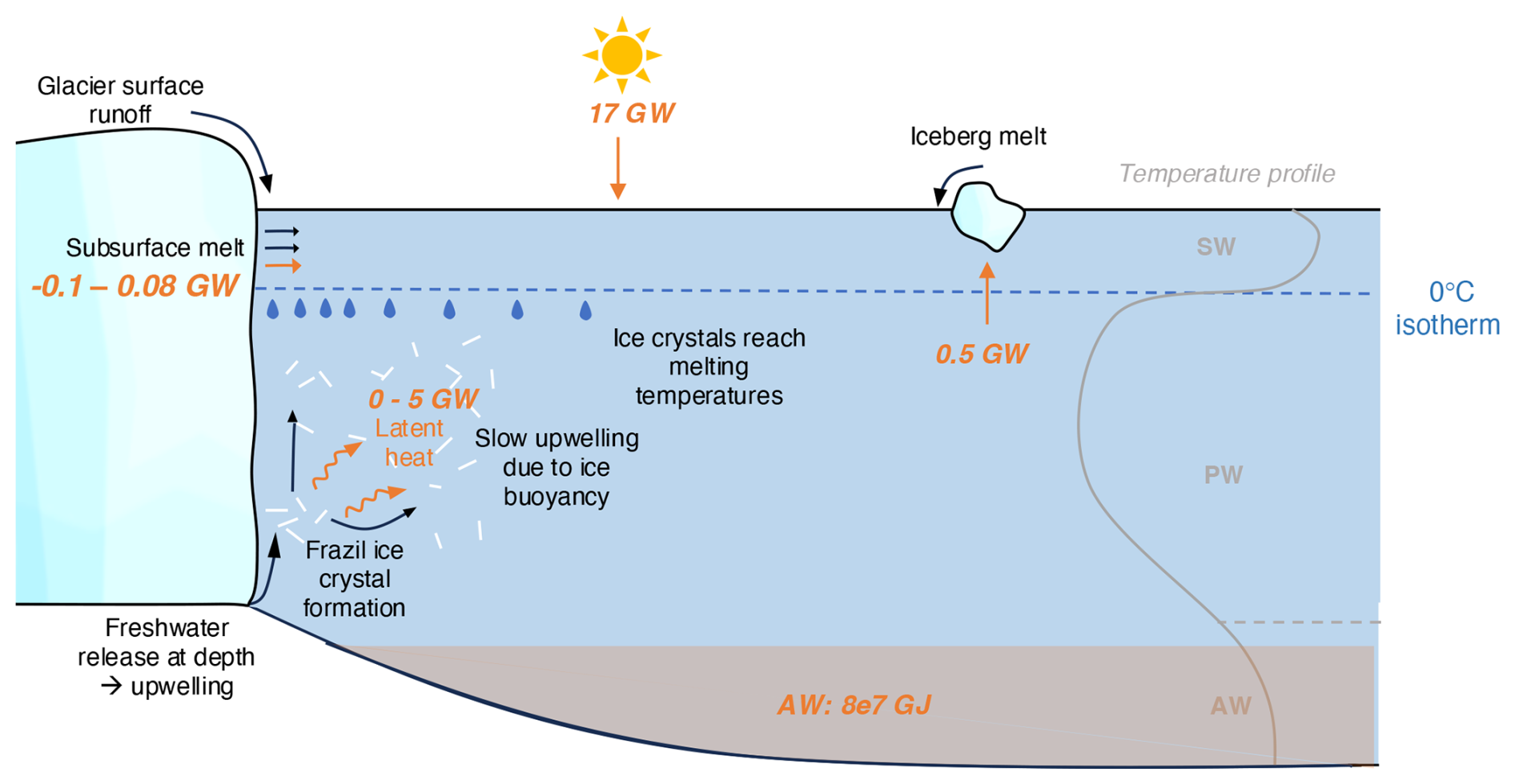
Figure 8 Schematic picture of our interpretation of the data depicting glacial meltwater refreezing and frazil ice crystal formation in the Polar Water layer. Orange arrows indicate the sources of heat flux, including glacier meltwater release (left), atmospheric heating (top) and iceberg melt (right), with their associated estimated values. The bottom light orange water body represents the heat stored in the Atlantic Water layer. A sketch of a typical measured temperature profile with the water types is included in grey, and the upper 0 °C isotherm is shown in blue.

3.5 Heat budget

A heat budget estimate was made to assess the different heat sources in Dickson Fjord. A similar approach was used by Bendtsen et al. (2015), where the authors conducted energy budget calculations for Kangersuneq. For these calculations, we assumed a stagnant water body in the fjord due to the absence of data on in-fjord water flows, which are challenging to obtain because moorings are often lost due to icebergs and other environmental factors.

For the heat balance estimates, the meltwater flux estimates by Karlsson et al. (2023) were used. They combined different data sets to give an estimate of the solid-ice discharge and surface and basal melt of the Hisinger glacier for the month of August every year between 2010 and 2020. Since August 2022 basal and surface melt have not been assessed yet, and these values do not seem to vary too much between years; the 2010–2020 August averages of these quantities were used for computations. These equal 3.6 ×10⁷ m³ for surface melt and 2.6 ×10⁶ m³ for basal melt. Important to note is that the surface melt values also represent the surface meltwater that is discharged at depth through glacial channels. Once the volume flux into the fjord is known, the following equation was used to compute the heat flux q:

$$\begin{array}{}\text{(4)}& q=\mathit{\rho }{c}_{p}Q\mathrm{\Delta }\mathit{\theta },\end{array}$$

with Δθ the difference between the water temperature of the in- or outflowing water and the ambient water, Q the volume flux, and ρ and c_p the density and specific heat capacity of the in- or outflowing water, respectively. The heat sources taken into account in this heat budget are the atmospheric heat (radiative, latent and sensible heat), the heat loss into melting solid ice discharge, the heat from surface glacier runoff, subglacial discharge and basal melt, and the potential latent heat from frazil ice crystal formation.

3.5.1 Atlantic Water layer heat

Assuming that the Atlantic Water layer has limited interaction with the glacier terminus and minimal heat exchange with the water bodies above, since the terminus does not reach Atlantic Water layer depths, this layer was excluded from the heat budget calculations. Nevertheless, its total heat content was estimated to highlight the substantial thermal energy stored within. This stored heat could become relevant during significant events such as substantial calving, potentially causing interactions between this layer and the overlaying water. For our heat budget calculations, the surface area of the fjord is approximated as 116 km², with an average depth of approximately 200 m, amounting to a total volume of around 23.2 km³.

3.5.2 Atmospheric heat

Through the on-land observatory, the 24 h averaged net incoming radiation measured at Ella Island from 21 to 31 August 2022 was obtained, which equals 123.4 W m⁻². Additionally, a mean August Atlantic Ocean albedo at 70° N (Payne, 1972) of 0.09 was found. Assuming minimal ice coverage in Dickson Fjord, this value is used for the energy influx calculation, resulting in an energy influx from radiation of approximately 13.0 GW. From the Zackenberg measurement station, we obtain an August average latent heat flux of −25.6 W m⁻² and a sensible heat flux of 61.5 W m⁻², measured at 2.5 m height near the fjord water. The total sensible and latent heat fluxes over the area of 116 km² amount to 7.1 and −3.0 GW. Subtracting the latent heat values from the incoming radiative heat flux and adding the sensible heat flux (as the sea surface temperature is colder than the atmosphere), the total atmospheric heat contribution was estimated at 17.1 GW.

3.5.3 Solid ice discharge heat loss

The energy that goes into melting glacial icebergs was computed using iceberg calving estimates, since this ice will be melted by the warm surface waters. According to computations by Karlsson et al. (2023), 3.64 ×10⁶ m³ (equivalent to approximately 9.7 m from the ice front) of ice calved off in August 2022. Assuming all this ice melts and using a latent heat of fusion of approximately 3.34 ×10⁸ J m⁻³, the heat rate going towards iceberg melting amounts to approximately 0.45 GW.

3.5.4 Glacial meltwater heat

As surface melt can be released in two ways, surface glacier runoff and subglacial discharge, the heat impact of this meltwater varies based on its discharge location. Due to this variability, a range of estimates was computed for the heat contributions of these meltwaters. To obtain this range, the heat contribution was computed for two scenarios: one where all surface melt is discharged at the surface (where ambient water temperatures are higher, resulting in a negative heat flux), and another where all meltwater is discharged at the coldest part of the Polar Water layer (resulting in a maximum heat contribution from this meltwater). For the first scenario, assuming all 3.6 ×10⁷ m³ is discharged at the surface and a Δθ of 2 °C, a total heat flux of −0.11 GW in August 2022 was obtained using Eq. (6). For the second scenario, assuming the meltwater discharged is around 0 °C, a specific heat capacity and density of, respectively, 4215 J kg⁻¹ K⁻¹ and 1000 kg m⁻³ were found, amounting to a total heat flux of around 0.08 GW in August 2022. Therefore, the heat flux due to glacial meltwater release in August 2022 was estimated to be in the range of −0.11–0.08 GW.

3.5.5 Frazil ice crystal latent heat

Since it remains unknown whether the frazil ice crystal formation occurs, as well as the quantity of ice crystals that are present in the water body, only a potential energy range can be estimated. For the upper limit, the sum of the surface and basal meltwater estimates was used, which equals 3.86 ×10⁷ m³. Assuming that all these crystals remain frozen and a latent heat of 3.34 ×10⁸ J m⁻³, this amounts to a maximum heat flux of 4.8 GW in August 2022. It is crucial to note that if the meltwater refreezes, the liquid state no longer contributes to the heat budget. Consequently, the values for surface glacier runoff and subglacial discharge are tied to the latent heat values. The average in-fjord depth of the water body was taken as 450 m, therefore estimating the total Atlantic Water volume to be 29 km³. Figure 2 shows a salinity of 34.6 and temperature value of 0.7 °C in the Atlantic Water layer at 300 m depth. Using these values, a specific heat capacity and density of 3979J kg⁻¹ K⁻¹ and 1029 kg m⁻³ were found, resulting in a heat content of approximately 8.3 ×10⁷ GJ.

In Fig. 8, a schematic illustrates the combined heat contribution estimated in this section. Whilst this offers an initial understanding of the heat sources and their magnitudes, it is crucial to acknowledge the numerous assumptions and estimates embedded in the calculations. Nevertheless, the heat budget estimate indicates that, apart from the latent heat release attributed to potential meltwater refreezing, there does not appear to be a heat source contributing to the temperature rise within the Polar Water layer. Comparing our findings to those of Bendtsen et al. (2015), we observe that our heat source estimates are significantly smaller. This is likely due to the much smaller surface area in our Dickson Fjord calculations (116 km² in Dickson vs. 400 km² in Kangersuneq).

4 Conclusions

This study aimed to understand the complex ice–ocean processes within Dickson Fjord during peak summer melt conditions (August 2022). By combining hydrographic and stable water isotope observations at various depths and locations, we investigated the fate of subglacial meltwater in a fjord dominated by cold Polar Water.

Bathymetry measurements showed that the terminus is exclusively in contact with surface waters and cold Polar Water. Since the seawater temperatures in the Polar Water layer are below the freshwater freezing point, we hypothesise that meltwater refreezes once it is released at depth. This refreezing process potentially led to the formation of frazil ice crystals, which release latent heat to the surrounding water. These ice crystals slowly float to the surface due to their buoyancy and melt once they reach freshwater melting temperatures, releasing freshwater into the fjord. This process is illustrated in Fig. 8 and is similar to the platelet ice crystal formation described by Hoppmann et al. (2020), with the key difference being that in our case, the primary freshwater source is surface freshwater released at depth rather than basal melt. The temperature and salinity data revealed a three-layer stably stratified water body: a fresh, warm surface layer; an underlying cold Polar Water layer; and a warm, saline Atlantic Water layer at the bottom. The glacier terminus was primarily in contact with cold Polar Water near the freezing point, with an increase in Polar Water layer temperature closer to the terminus. Water fraction calculations indicated that this heat increase could not be solely due to liquid meltwater release, with an unaccounted heat estimated at 1.1 ×10¹⁶ J. Isotope partitioning suggested an in-fjord meltwater distribution of 22 % surface meltwater, 31 % subsurface meltwater and 47 % Polar Water layer meltwater, though this likely underestimates surface meltwater due to unaccounted sea ice formation.

The process of meltwater refreezing at depth would explain the excess heat present in the Polar Water layer, attributed to latent heat release. To account for the excess heat estimate in the Polar Water layer through frazil ice crystal formation, the total volume of meltwater required to refreeze amounts to 3.4 ×10⁷ m³, assuming a stagnant water body. This refreezing process also clarifies the subsurface depleted d¹⁸O signal in Fig. 5a, occurring around the freshwater freezing line where ice crystals melt and release glacial freshwater. Comparing this refreeze volume to the meltwater release estimates by Karlsson et al. (2023), this value is close to the surface meltwater estimate of 3.6 ×10⁷ m³ in August 2022. While this hypothesis aligns with low Polar Water temperatures and could explain the excess heat observed in the isotopic sections, more research is required to validate the presence of frazil ice crystals in the Polar Water body. In situ observation of these crystals is crucial for validation, although obtaining these observations is challenging.

Further studies are needed to provide more precise estimates of subsurface freshwater inflow and fjord outflow to determine if the Polar Water layer heat increase can indeed be explained by meltwater refreezing (frazil ice formation). Simulations of freshwater release into saline waters and detailed fjord system models could enhance our understanding of fjord heat budgets and current flows. Additionally, research focusing on in-fjord currents, especially in- and outflows at different depths, could offer valuable insights into the fjord's heat content and dynamics. Continuous isotopic water sampling across various depths and locations would help identify the movement and outflow patterns of glacial meltwater. In conclusion, this study sheds light on the freshwater dynamics and glacier–ocean interactions within Dickson Fjord during peak summer melt conditions. The observed phenomena of frazil ice formation and unresolved questions underscore the need for further research to fully understand the complexities of glacial meltwater behaviour.

Appendix A: Thermal image Dickson Fjord

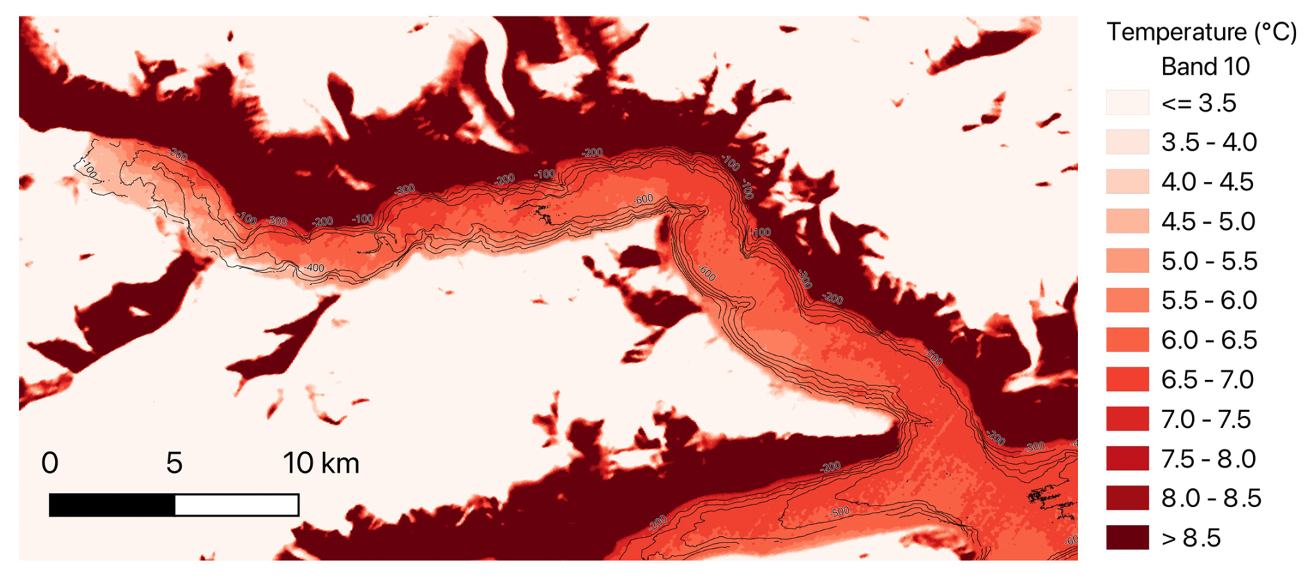
Figure A1 Thermal image of Dickson Fjord, including high-resolution 100 m bathymetry contour lines. The thermal image was generated using satellite data from the Landsat 8 OLI/TIRS satellite (Band 10) on 20 August 2022.