Impact of modulating surface heat flux through sea ice leads on Arctic sea ice in EC-Earth3 in different climates

This sensitivity study examines the impact of modulating surface sensible heat flux over leads – open-water areas within sea ice cover – to approximate finer-scale processes that are often underrepresented in climate models. We aim to assess how this parameterization (referred to as ECE3L) influences the persistent positive bias in Arctic sea ice (concentration and thickness) in the global climate model EC-Earth3 (ECE3). We performed two pairs of 50-year simulations using 1985 (cold-climate) and 2015 (warm-climate) forcing, with the latter characterized by thinner ice and weaker atmospheric boundary layer stability during winter. Our results show that modified heat flux alters surface air temperatures in the Arctic, with minimal impact on lower latitudes. The changes are more pronounced in the cold-climate experiment, particularly during Arctic winter. We also performed a historical ensemble comparison between ECE3L and ECE3 over a transient-climate period (1980–2014). We found that the spatial patterns in mean sea ice changes in the transient climate closely resembled those observed in the cold-climate experiment. However, the reduction in the total sea ice area and volume in ECE3L relative to ECE3 was nearly 4 times greater in the cold climate compared with the transient climate. This suggests that amplified heat flux through leads is less effective in a warming climate with decreasing winter stratification. Notably, ECE3L shows closer alignment with observational data and refines the declining sea ice volume trend overestimation in ECE3, reducing overestimated ensemble variability caused by excessive sea ice. This, in turn, amplifies sea ice sensitivity to Arctic warming, particularly in the marginal ice zone. These findings emphasize the importance of accurately representing surface heat flux through sea ice leads, which plays a critical role in capturing the influence of atmospheric stability on sea ice dynamics and regional Arctic amplification.

1 Introduction

Sea ice influences thermal interactions between the ocean and atmosphere by acting as an insulating barrier and reflective surface. An accelerated reduction in Arctic sea ice cover (extent and thickness) leads to increased solar absorption by the ocean (i.e. ice–albedo feedback mechanism), which in turn intensifies surface warming (Bhatt et al., 2014). As a result, Arctic warming rates have nearly quadrupled compared to the global average since satellite observations commenced in 1979 (Rantanen et al., 2022). The Arctic's rapid warming can increase the melting of the Greenland ice sheet, raise global sea levels, extend and intensify Arctic fire seasons, speed up permafrost thaw, and alter weather patterns in the heavily populated mid-latitudes regions of the Northern Hemisphere (AMAP, 2021; Eyring et al., 2021; Thomas, 2017; Johannessen et al., 2020).

Accurate modelling of Arctic sea ice is essential for understanding and predicting the impact of climate change. However, several Earth system models that contributed to the Coupled Model Intercomparison Project Phase 6 (CMIP6; Eyring et al., 2016), including EC-Earth3, tend to simulate excessive sea ice in winter and an early minimum in August (Keen et al., 2021; Doescher et al., 2022) instead of September, as indicated by observational, satellite-based datasets (Cavalieri et al., 1996; Stroeve et al., 2014; Fox-Kemper et al., 2021). The CMIP6 multi-model mean captures the observed decline in Arctic sea ice in general, while substantial variability exists both among different models and among ensemble members of the same model (Lee et al., 2023), highlighting internal variability as a key source of uncertainty in decadal trends (Dörr et al., 2023). A major challenge lies in ice thickness representation: models with thicker ice tend to exhibit a faster decline in sea ice volume than those with thinner ice, increasing uncertainty in reproducing the overall rate of decline (Lee et al., 2023; Massonnet et al., 2018). Ice thickness also influences feedback mechanisms, such as the ice–albedo effect, where thinner ice and earlier melt expose open water, accelerating warming (Bhatt et al., 2014). Additionally, missing processes like surface heat flux over sea ice leads, which mediate ocean–atmosphere heat exchange in winter, can amplify local warming (Esau, 2007; Marcq and Weiss, 2012). These factors contribute to uncertainties in modelling Arctic warming and in projecting future sea ice evolution and its climate impacts (Wunderling et al., 2020).

Several studies have highlighted the need for climate models to reduce biases in the historical climate mean state to improve projections of sea ice changes (Massonnet et al., 2018; Docquier and Koenigk, 2021; Keen et al., 2021; Kay et al., 2022). Particularly in a warming climate, the thinning of sea ice and snow cover increases the importance of thermodynamic processes, involving heat and energy exchange between the sea ice, atmosphere, and ocean surface (Massonnet et al., 2018; Landrum and Holland, 2022; Webster et al., 2021). Deser et al. (2010) demonstrated a connection between Arctic temperature inversion and sea ice loss, suggesting that the strong wintertime marine temperature inversion observed from 1980 to 1999 will diminish by 2080–2099. However, the presence of a positive bias in sea ice mean states can have profound consequences for the atmosphere, leading to unrealistic stable atmospheric stratification and ultimately damping the modelled sea ice sensitivity to external forcing.

In this study, we hypothesized that modulating upward heat flux through leads can help mitigate the seasonal bias in the coupled EC-Earth3 model and improve the simulation of Arctic sea ice. This hypothesis is based on the understanding that the absence of a parameterization for turbulent exchange over leads in global climate models hampers adequately capturing the exchange of heat and energy between the atmosphere and the ocean through these crucial areas (Esau, 2007; Marcq and Weiss, 2012). Consequently, this deficiency may result in an early onset of stable stratification and an extended period of sea ice growth.

Implementing a new modulating factor to the Norwegian Earth System Model (NorESM), in its atmosphere-only model configuration (https://blue-action.eu/, last access: 20 July 2025, Davy and Gao, 2019), significantly advanced our understanding of how heat fluxes through sea ice leads affect the Arctic's surface energy balance. This factor takes seasonal variations into account and varies based on the stability of the atmospheric boundary layer, increasing heat flux through leads to warm the air above during winter and dampening it during summer. Although the modulating factor shows promise in addressing known seasonal biases, its long-term climate impacts remain uncertain due to potential changes in atmospheric stability and the spatial distribution of leads (Deser et al., 2010), highlighting the need for further investigation.

To address these, we propose implementing the modulation factor into a coupled climate model. Specifically, this will allow us to investigate whether an amplified heat flux through sea ice leads in winter may better represent the transition to a warmer Arctic with less perennial sea ice, potentially reducing the importance of leads under climate change. Moreover, we aim to assess whether this modification can improve the sensitivity of climate models to external forcing in the Arctic. To do so, we will analyse changes in the trends in key essential climate variables (sea ice extent, area, volume, and surface air temperature) during a period of rapid Arctic change (1980–2014; Schweiger et al., 2019) due to the inclusion of the lead scheme. We will also identify the added value of this modification in reducing model bias on a regional scale.

2 Methods

2.1 Empirical relationship between surface heat flux amplification (A_lead) and sea ice leads

An empirical parameterization, introduced by Davy and Gao (2019) for the NorESM model, defines the relationship between surface sensible heat flux (SSHF) amplification and sea ice leads. This approach builds upon turbulence-resolving simulations of heat fluxes over leads of different widths and atmospheric stability (Esau, 2007), combined with satellite-derived lead width distributions (Marcq and Weiss, 2012), to better represent sub-grid-scale processes. Their sensitivity study, conducted using an atmosphere-only model configuration, shows an improved characterization of SSHF in regions with partial sea ice cover.

The amplification factor A_lead depends on atmospheric stability, quantified via the convective boundary layer length scale (λ_CBL) and sea ice concentration (SIC), with the latter defined as the fractional area of sea ice within a grid cell (in percent). The state-dependent λ_CBL is derived from an empirical formula based on the instantaneous air temperature gradient θ (200–300 m) in the atmospheric model. For grid cells with SIC≥90 %, A_lead reaches its maximum value (linearly interpolates to 1 for SIC≤70 %). A full derivation of this parameterization, including the governing equations and parameter choices, is provided in Appendix A.

2.2 The coupled EC-Earth3 model with implementation of A_lead

In our study, we used a well-documented, state-of-the-art global climate model EC-Earth3 (version v3.3), which is the model version that contributed to CMIP6 (Doescher et al., 2022). This model comprises three main components: atmosphere, ocean, and sea ice. The atmospheric component incorporates the Integrated Forecast System (IFS cycle 36r4) developed by the European Centre for Medium-Range Weather Forecasts (ECMWF), with a horizontal grid of TL255 and 91 vertical model levels. The ocean component uses version 3.6 of the Nucleus for European Modelling of the Ocean (NEMO3.6) embedded with version 3 of the Louvain-la-Neuve sea Ice Model (LIM3; Rousset et al., 2015). The NEMO-LIM3 set-up uses a nominal 1° resolution horizontal grid (i.e. ORCA1) and 75 vertical levels. In particular, the LIM3 sea ice model adopts an ice thickness distribution framework to deal with fine-scale ice thickness variations (Rousset et al., 2015).

EC-Earth3, hereafter referred to as ECE3, exhibits an Arctic sea ice bias in its mean state. While the total area of Arctic sea ice aligns well with satellite observations, there are generally large positive biases in the total volume of Arctic sea ice (Doescher et al., 2022), compared to the Pan-Arctic Ice–Ocean Modeling and Assimilation System (PIOMAS; Zhang and Rothrock, 2003), a reanalysis that has been extensively validated (Stroeve et al., 2014; Wang et al., 2016) and broadly used by the community as a reference product (Davy and Outten, 2020; Keen et al., 2021). In September, the model shows an evident overestimation of the Arctic sea ice thickness (SIT), with a bias of up to 2 m, while in March, ECE3 overestimates it in the central Arctic but underestimates it in the Bering and Kara seas relative to PIOMAS (see Fig. 13 in Doescher et al., 2022).

To alleviate the bias in the Arctic sea ice and assess its consequences on the global climate system, we incorporated the factor A_lead into the SSHF calculations within the coupled ECE3 framework, addressing a topic that has not been extensively explored in previous studies (Davy and Gao, 2019). A_lead is applied globally on the sea ice of both poles and updated at each model time step with the instantaneous conditions of the lower-level air temperature gradients θ and SIC on the atmospheric model grid. The EC-Earth3 simulations with the implementation of A_lead are hereafter referred to as ECE3L.

In ECE3L, all surface fluxes are computed in the atmosphere using state variables from the ocean–atmosphere interface and then remapped to the ocean and sea ice components via the OASIS3-MCT coupler (Doescher et al., 2022). The modulating factor, A_lead, influences only the sensible heat flux in the surface atmosphere by either amplifying or damping it over leads, depending on atmospheric stability. This adjustment can result in increases of up to 1.2, enhancing surface heat exchange over sea ice where SIC exceeds 70 %, particularly during winter. Conversely, in summer, the factor decreases from 1 to 0.9, leading to a reduction in surface heat exchange and producing the opposite effect on the surface atmosphere (see Fig. S1 in the Supplement and Sect. 3.2).

2.3 CMIP6 historical simulations and the comparison strategy

We first performed a pairwise comparison of single simulations between ECE3L and ECE3 (i.e. with/without A_lead) in cold and warm climates (hereafter referred to as ExpCold and ExpWarm, respectively). Here, we distinguished the warm-climate scenario by its characteristics of thinner ice and weaker atmospheric boundary layer stability during winter compared to the cold climate (Fig. 1). To exemplify the contrasting conditions, we arbitrarily selected the years 1985 and 2015 to represent the warm and cold periods, respectively. The coupled simulations used the CMIP6 historical external forcing from the given year (including solar radiation, greenhouse gas concentrations, aerosols, and land use). The ocean and atmospheric variables still freely evolve in the simulation without being constrained. The initial states are from one of the members of the ECE3 CMIP6 historical ensemble (see Fig. 3 by Doescher et al., 2022), specifically r5i1p1f1. We selected initial conditions from the historical simulation of r5i1p1f1 on 1 January in 1985 and 2015, respectively, and repeated external forcing for the respective years in a 50-year cycle. For each simulation, the first 20 years were designated as the spin-up period, with the subsequent 30 years for comparison purposes. We investigated (1) whether implementing the new scheme in coupled climate simulations would result in any global impact and (2) if this impact is influenced by the state of Arctic sea ice.

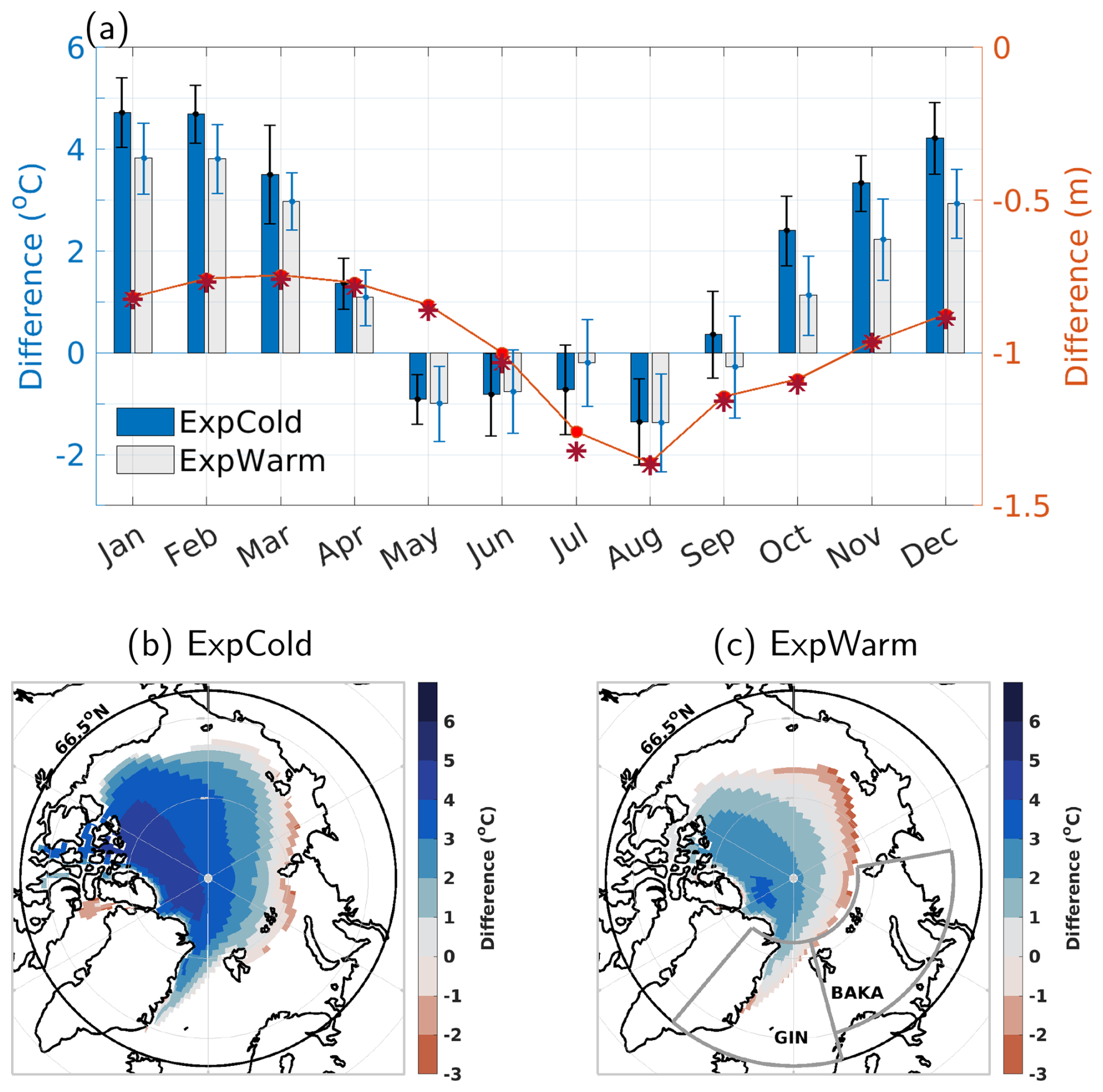
Figure 1 The ECE3 baseline simulation. Panel (a) presents the annual cycle of air temperature differences between the 850 and 1000 hPa levels over Arctic sea ice for the ExpCold (dark blue) and ExpWarm (light grey) scenarios. Error bars indicate 1 standard deviation of the 30-year variability. The temperature data are area-averaged for regions with a sea ice concentration (SIC) ≥70 % in the Arctic Ocean (66.5–90° N). Additionally, the 30-year mean differences in sea ice thickness between ExpWarm and ExpCold are shown on the right y axis, using solid circles (SIC≥70 %) and stars (SIC≥80 %). Panels (b) and (c) illustrate air temperature differences in October using 30-year averages in ExpCold and ExpWarm, respectively. The thick black line indicates the Arctic Circle (66.5° N), within which the sea ice area for SIC ≥70 % is calculated in panel (a) for each month. The thick grey lines mark the Greenland–Iceland–Norwegian (GIN) seas (40° W–15° E, 66.5–82° N) and the Barents and Kara (BAKA) seas (15–100° E, 70–82° N) used in Fig. 12.

Next, we investigated how the presence of leads in Arctic sea ice affects the coupled climate system in a transient climate, particularly during significant Arctic warming due to climate change (1980–2014). Specifically, we focused on two key questions:

1. How might the importance of these open leads change during winter due to shifts in atmospheric stability?

2. How does the differing sea ice evolution influence the modelled Arctic warming?

To address these, we performed a 20-member ensemble simulation using ECE3L and compared it with a 20-member ECE3 ensemble (Doescher et al., 2022), both utilizing the same historical forcing from CMIP6. The 20 members used were selected from the broader 25-member ECE3 CMIP6 ensemble (i.e.  r1–r25i1p1f1, as shown in Fig. 3 of Doescher et al., 2022). Only 20 out of 25 members are publicly accessible through the Earth System Grid Federation (ESGF, https://esgf.llnl.gov, last access: 20 July 2025). These simulations were performed by the EC-Earth consortium following the CMIP6 protocol (Eyring et al., 2016) for historical simulations of CMIP6 (1850–2014).

To generate the ECE3L ensemble, we started with the initial conditions of two ECE3 members from 1960 (i.e. r5i1p1f1 and r8i1p1f1), applied the A_lead factor, and ran each simulation through a 15-year spin-up period. From 1975, we populated each of these simulations into 10 separate runs by introducing small random perturbations (around 10⁻⁵ K) to the 3D temperature field in the atmosphere, which caused ensemble members to diverge within days (see Sect. 4.1 and Fig. S5). This resulted in a 20-member ECE3L ensemble that ran until 2014. Details of the experimental set-up are summarized in Table 1.

Table 1 Summary of the pairwise experiments (ECE3 vs. ECE3L).

^* ECE3 is a 25-member (r1–r25i1p1f1) ensemble (Doescher et al., 2022), with the realizations 6, 9, 11, 13, and 15 not being publicly accessible.

2.4 Validation data and metrics

The model evaluation covers the 1980–2014 period, aligning with the availability of satellite-based observational sea ice datasets in the Arctic. Our analysis involves comparing the two ensemble simulations. First, we calculate the bias, which was derived from the differences between the ensemble mean and the observed data. Second, we quantify the improvements by calculating the differences between the ECE3L and ECE3 ensemble means. These calculations enable us to evaluate the model's ability to replicate observed conditions and to understand how the inclusion of A_lead influences its performance.

For sea ice thickness, we relied on the PIOMAS reanalysis. Although PIOMAS is not strictly an observational dataset, it is a valuable reference because it has been well validated against observations (e.g. Stroeve et al., 2014; Wang et al., 2016). It also provides well-quantified measures of uncertainty (Schweiger et al., 2011) and is commonly used to evaluate climate models (Davy and Outten, 2020; Keen et al., 2021). For sea ice concentration, we used two independent observational datasets: one referred to as NSIDC-0051, which is derived from passive microwave data and has been processed using the NASA Team algorithm (Cavalieri et al., 1996), and the other referred to as OSI-450a, known as the global sea ice concentration climate data record, version 3.0 (2022). The latter dataset was sourced from the Ocean and Sea Ice Satellite Application Facility (OSI SAF). Given that PIOMAS assimilates sea ice concentration data from NSIDC products, we considered NSIDC-0051 to be the primary reference. The data from OSI-450a served as a secondary reference.

For model evaluation, we maintained consistency by regridding all sea ice data, from both climate models and observations, to the NSIDC-0051 polar stereographic grid with a 25 km spatial resolution, following Lin et al. (2021). We calculated sea ice area, extent (SIC>15 %), and volume (i.e. multiplying sea ice area by the sea ice thickness) across the entire Northern Hemisphere ice-covered region using monthly mean data from 1980 to 2014. To evaluate the accuracy of modelled sea ice edges compared to observations, we used the integrated ice-edge error (IIEE) metric introduced by Goessling et al. (2016), applying a criterion of SIC = 15 % to define the sea ice edge. The IIEE quantifies the total area where the modelled SIC differs by more than 15 % from the reference data. It accounts for regions where the model either overestimates (O) or underestimates (U) SIC relative to the 15 % threshold. In summary, the IIEE is calculated as the sum of these areas: $\text{IIEE}=O+U$. This metric offers valuable insights into how well the modelled sea ice edges align with observational references (e.g. Ponsoni et al., 2023).

To evaluate how changes in surface heat flux can influence temperature patterns and trends in the Arctic and globally, we selected four global surface temperature datasets as reference fields. These datasets include ERA5 (Hersbach et al., 2020), NCEP2 (Kanamitsu et al., 2002), and JRA-55 (Kobayashi et al., 2015), which are three atmospheric reanalysis datasets providing air temperature at 2 m (T2m). Additionally, we use the Berkeley Earth Land/Ocean temperature dataset (BEST; Rohde and Hausfather, 2020), which is different from reanalysis datasets as it combines its own land surface temperature records with air temperature data and utilizes the HadSST4 dataset for sea surface temperatures (SSTs; Titchner and Rayner, 2014). Following Rantanen et al. (2022), local Arctic amplification is defined as the ratio of the temperature trend at each grid point to the global mean temperature trend, and the Arctic region is defined as the area encircled by the Arctic Circle (66.5–90° N). The slopes of linear trends in surface temperatures used least-squares fitting for the annual mean values. In this study, our main objective is to evaluate how amplified heat flux reduces the overestimation of modelled sea ice in the Arctic. Therefore, we do not include an analysis on the underestimated sea ice in the Antarctic.

3 Cold vs. warm climate

3.1 Atmospheric stability and sea ice variability

The turbulent processes over sea ice are affected by the temperature difference between the air and the ice surface, which is influenced by sea ice concentration (lead cover) and ice thickness (Lüpkes et al., 2008). In the ECE3 (baseline) simulations, the occurrence of the low-level winter temperature inversion is defined as positive air temperature differences between 850 and 1000 hPa, following the method of Deser et al. (2010). In Fig. 1a, the winter temperature inversion over Arctic sea ice (SIC≥70 %) is considerably weaker and shorter in ExpWarm compared to ExpCold on a 30-year average. Particularly during the early freeze-up months (October and November), mean differences in a warmer climate are nearly half the size of those in a colder climate, with the central Arctic pack ice (SIC≥70 %) experiencing over 1 m of thinning and more than 2×10⁶ km² of shrinkage during summer (Fig. 1b and c) compared to ExpCold. The comparison between two baseline simulations suggests that the effect of parameterizing turbulent process on sea ice becomes less pronounced during Arctic warming, likely due to a reduction in the strength and duration of winter temperature inversion.

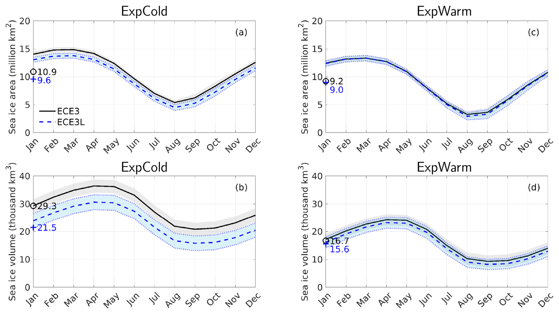
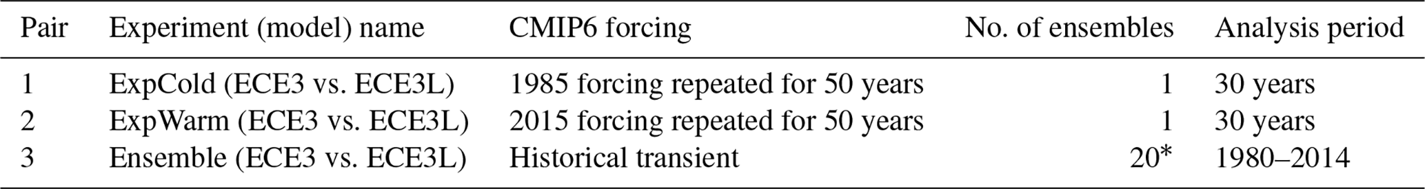
Figure 2 Comparison of the Arctic's annual cycle under a constant forcing between ECE3 (solid black line) and ECE3L (dashed blue line) for (a) sea ice area and (b) sea ice volume. Simulations are performed for ExpCold, characterized by thicker ice and stronger stability of the atmospheric boundary layer during winter in the Arctic Ocean. Values are shown as the mean (thick line) and 1 standard deviation (shaded area) over the last 30 years. The full time series of simulations is shown in Fig. S2. Panels (c) and (d) are the same as panels (a) and (b) but for ExpWarm with thinner ice and weaker static stability. SIA and SIV are calculated with the cdficediags tool (from CDFTOOLS 3.0). Numbers and symbols indicate the 30-year mean for the respective variables for ECE3 (open black circles) and ECE3L (blue crosses). The mean differences are statistically significant (p<0.05, two-sided t test) in panels (a), (b), and (d) but not in panel (c).

The 30-year mean Arctic sea ice area (SIA) and sea ice volume (SIV) in the ECE3 simulations for ExpWarm account for 84 % and 57 % of those for ExpCold, respectively (Fig. 2). This is equivalent to a decrease in the mean thickness, defined as the total SIV divided by SIA, from 2.7 to 1.8 m. In the ECE3L simulations, the 30-year mean changes caused by modified heat fluxes through leads are less pronounced in ExpWarm than in ExpCold (Fig. 2). Specifically, SIA is 2 % (12 %) less in ECE3L than in ECE3, while SIV is 7 % (27 %) less in ECE3L during the 30-year time frame for ExpWarm (ExpCold). The mean differences are statistically significant (p<0.05 in a two-sided t test), except for SIA in ExpWarm (p>0.05 in Fig. 2c). The results support our hypothesis that the model's response to the modulation of surface heat flux can be influenced by the winter temperature inversion and the extent of thick ice (Fig. 1). In ExpCold, the modulation of heat fluxes in ECE3L consistently reduces SIA and SIV after the spin-up, leading to thinner ice compared to ECE3. In ExpWarm, however, ECE3L exhibits both increases and decreases in sea ice with minimal impact on overall thickness (see the full time series in Fig. S2). The interannual variability in ECE3L closely aligns with that of ECE3 across all months in both ExpCold and ExpWarm (Fig. 2), indicating that the parameterization does not alter the system's internal variability.

Globally, we find that the 30-year mean of global surface temperature in ExpCold is 0.21 °C higher in ECE3L than ECE3, which falls within the range of model variability across the ECE3 20 members of historical simulations (which is 0.24 °C for the respective year). Similarly, the change is only 0.02 °C higher between ECE3L and ECE3 in ExpWarm, relative to the model spread of 0.18 °C. This indicates that the change in global mean surface temperature induced by the modulation of heat flux over sea ice in ECE3L is within the range of natural variability represented by the model ensemble. In particular, the modification does not cause global surface temperature drift, and both models exhibit robust internal variability, as illustrated in Fig. S2c.

3.2 Local and remote influences of sea ice leads

The region with thick ice (2 m isoline in Fig. 3a and c) in winter is considerably smaller in ExpWarm compared to ExpCold. Consequently, the thinning of sea ice differs between these two climate scenarios. In ExpCold (Fig. 3b), it reaches a maximum of −1 m in the central Arctic, particularly in the region from north of Greenland to the Beaufort Sea. In ExpWarm (Fig. 3d), the largest reduction (−0.5 m) shifts to the central Arctic, north of the Laptev and East Siberian seas. This shift coincides with regions experiencing peak winter amplification of heat flux through leads (refer to Fig. S1a and c). This spatial pattern is governed by the prevailing conditions of atmospheric instability. In Fig. 4a and c, the sea ice cover shows similarities between ExpCold and ExpWarm in ECE3L. However, when compared to ECE3, there is a considerable reduction in sea ice concentration (where SIC<70 %) in the North Atlantic marginal ice zone in ExpCold, whereas there are only small changes in the Greenland Sea in ExpWarm, as illustrated in Fig. 4b and d. These findings suggest that overall sea ice thinning, particularly at the ice margins, is a key driver of the sea ice concentration reduction during Arctic winters. In these dynamic marginal zones, where the ice is often thin and fractured, even small reductions in thickness can lead to substantial decreases in ice extent. In contrast, the concentration in the central Arctic's pack ice remains close to 100 % during winter, even with thickness reductions of 1 m or more. This thinning at the margins coincides with a significant rise in surface air temperature by approximately 2° (Fig. 5), indicating a warmer atmospheric boundary layer extending southwards.

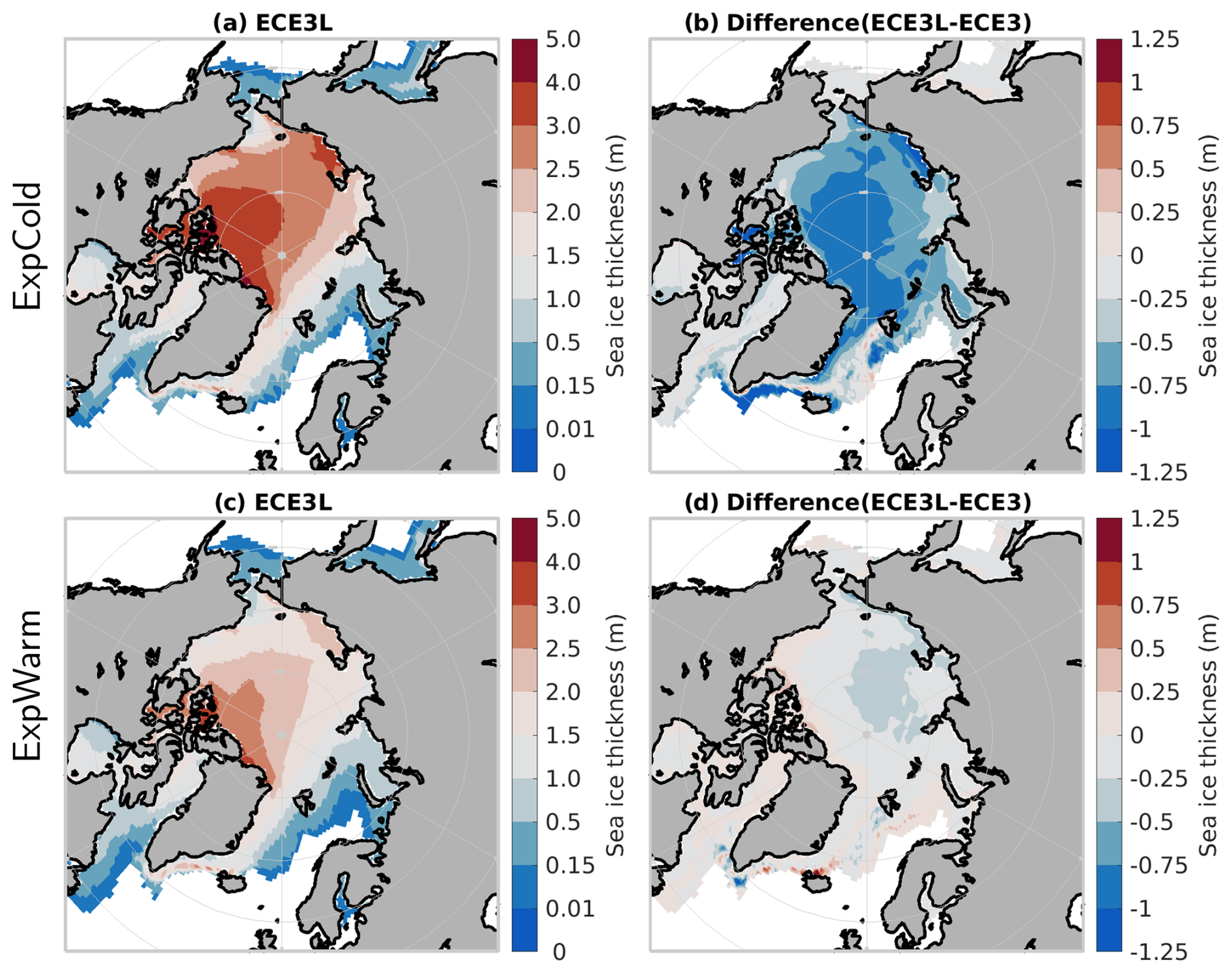
Figure 3 The late-winter (March) Arctic sea ice thickness under a constant forcing for ExpCold (a) ECE3L and (b) the ECE3L minus ECE3 differences. Panels (c) and (d) are the same as panels (a) and (b) but for ExpWarm. Values are shown as 30-year averages, as in Fig. 2. Note that a nonlinear colour scale is used in panels (a) and (c) to emphasize low ice thicknesses. Thicknesses under 0.01 m are not shown. Note that the PIOMAS domain is defined as SIT>0.15 m (see colour bar). The late-summer Arctic is shown in Fig. S3.

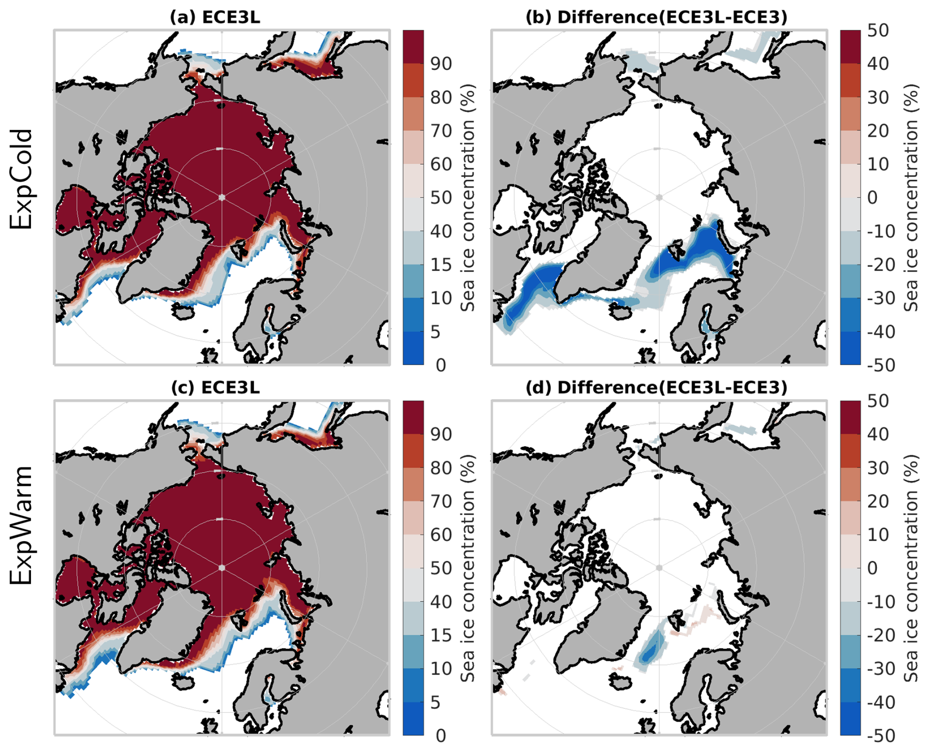
Figure 4 The late-winter (March) Arctic sea ice concentration under a constant forcing for ExpCold (a) ECE3L and (b) the ECE3L minus ECE3 differences. Panels (c) and (d) are the same as panels (a) and (b) but for ExpWarm. Values are shown as 30-year averages, as in Fig. 2. Note that a nonlinear colour scale is used to emphasize low ice concentrations. Concentrations under 5 % are not shown. The late-summer Arctic is shown in Fig. S4.

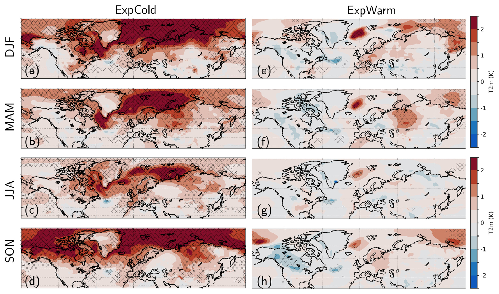
Figure 5 Seasonal differences in the 2 m temperature (in K) between ECE3L and ECE3 in the Northern Hemisphere (20–90° N) for ExpCold (a–d) and ExpWarm (e–h). Stippling indicates areas with statistically significant differences (p<0.05) as determined by a two-sided t test.

In Arctic summer (A_lead<1), sea ice thinning patterns remain consistent with winter (Fig. S3), indicating the dominant role of winter amplification. The thicker ice in the Pacific marginal seas compared to north of Greenland is present in both ECE3 and ECE3L and results from a known EC-Earth3 bias (Doescher et al., 2022), not the modulation effect (Fig. S3d), which applies only in the stratified central Arctic (Fig. 1). Additionally, there is a notable reduction in sea ice concentration of up to 30 % in ExpCold compared to less than 20 % in ExpWarm, as illustrated in Fig. S4. These results clearly show a reduction in the magnitude of heat flux amplification, corresponding to a decline in the mean states of sea ice as the climate shifts from colder to warmer conditions, observed in both the winter and summer months.

Statistically significant differences in the surface air temperature between ECE3L and ECE3 are noted at high latitudes in all seasons in ExpCold (Fig. 5), unlike in ExpWarm where the differences are minor. In regions with less sea ice in ECE3L compared to ECE3, the surface is warmer in ECE3L, especially in non-summer seasons. These findings underscore the role of sea ice in shaping polar surface temperatures. A warmer atmosphere can facilitate greater moisture convergence, increasing precipitation, especially in the Arctic. Therefore, variations in precipitation generally reflect the temperature differences between ECE3L and ECE3, with the magnitude being negligible (not shown), aligning with the findings of Kay et al. (2022).

4 Transient climate: comparison of historical ensemble simulations

4.1 Enhanced performance: reduced seasonal bias and narrower model spread

The ensemble mean of ECE3L consistently shows a lower sea ice area and volume than that of ECE3 throughout the annual cycle, with the largest differences noted during winter when the sea ice area and volume in ECE3 reach their peak (Fig. 6). The ensemble means show significant differences for both Arctic sea ice area and volume climatologies (p<0.05 in a two-sided t test). ECE3L more closely aligns with the observed seasonal cycle than ECE3. However, during the summer months (June–August), both models slightly underestimate sea ice area, with ECE3L showing a slightly larger mean difference of $-\mathrm{0.6}\times {\mathrm{10}}^{\mathrm{6}}$ km² compared to $-\mathrm{0.4}\times {\mathrm{10}}^{\mathrm{6}}$ km² for ECE3 in June. This underestimation aligns with a common bias across several coupled CMIP6 models, including ECE3, where the minimum summer Arctic sea ice area occurs in August rather than September (Keen et al., 2021; Doescher et al., 2022). Consequently, the largest biases are observed in September, amounting to 0.7×10⁶ km² for ECE3L and 1×10⁶ km² for ECE3. Both ensembles consistently overestimate the Arctic sea ice volume throughout the year, with positive monthly mean biases ranging from 6×10³ to 11.2×10³ km³ in ECE3L and from 7.8×10³ to 12.9×10³ km³ in ECE3. These biases are reduced year-round by the lead scheme; however, they are not significantly different from those in the ECE3 historical ensemble. The ensemble spreads range from 2.6×10³ to 3.2×10³ km³ in ECE3L and from 4.8×10³ to 5.5×10³ km³ in ECE3.

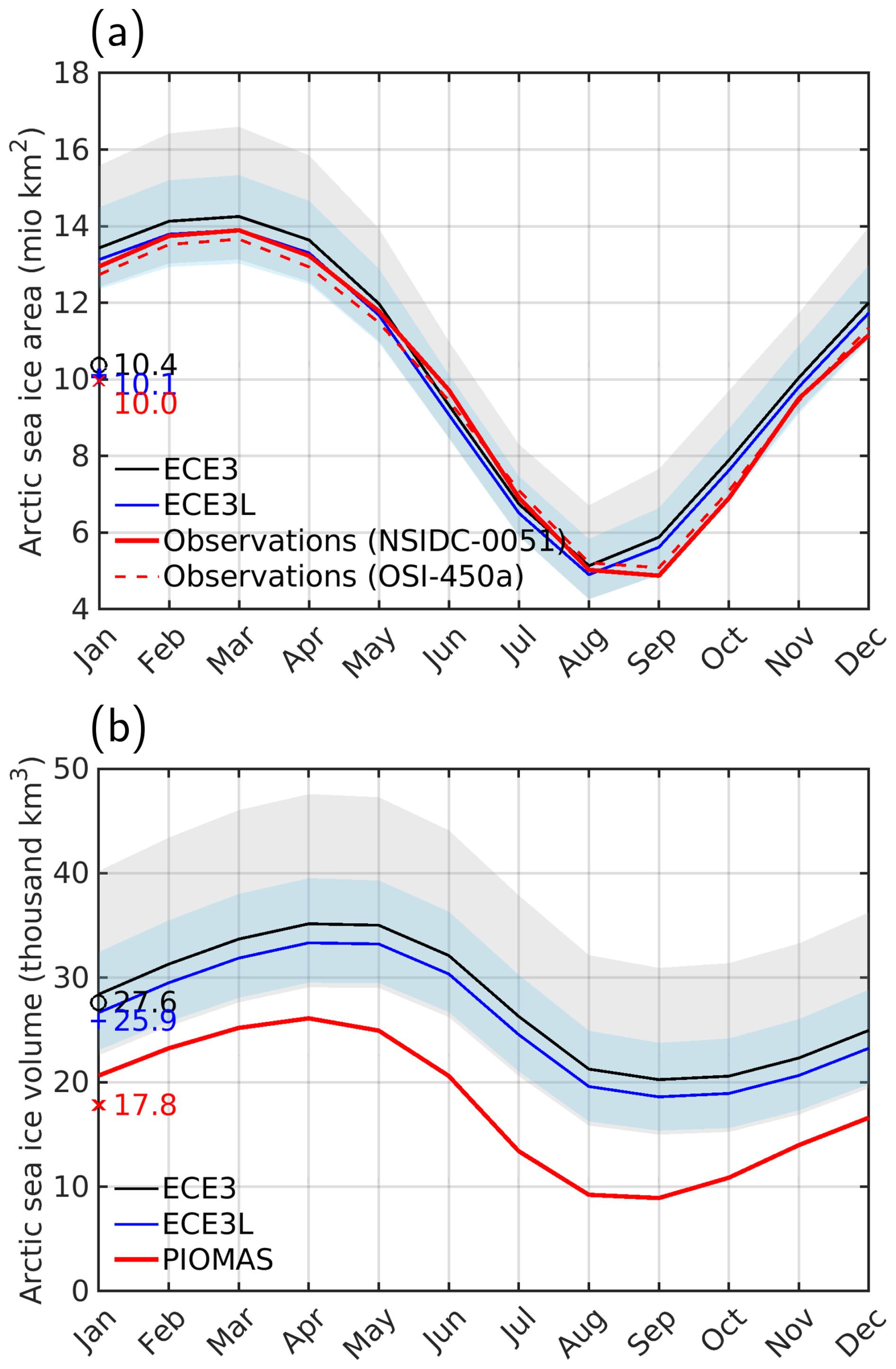
Figure 6 Comparison of the annual cycle in the transient climate (1980–2014) between ECE3 (black) and ECE3L (blue) for (a) Arctic sea ice area and (b) Arctic sea ice volume. Thick lines represent the ensemble means, while the shaded areas indicate the spread between the 5th and 95th percentiles across 20 ensemble members (grey for ECE3 and light blue for ECE3L). Observations for the sea ice area include the NSIDC and OSI-450a datasets, both remapped to the NSIDC-0051 grid. Sea ice volume is based on the PIOMAS domain criteria (thickness >0.15 m). The mean differences are statistically significant (p<0.05, two-sided t test).

Further comparisons highlight that the September Arctic sea ice extent in the ECE3L ensemble closely matches observations from 1980 to 2014, outperforming ECE3 (Fig. 7b). Across most years, ECE3L consistently shows a lower September sea ice extent than ECE3 (Fig. 8a). In March, the Arctic sea ice volume in ECE3L shows a closer alignment with the PIOMAS reanalysis, demonstrating its improved performance over ECE3 (Figs. 7c and d and 8b). In Fig. 8, the September sea ice extent and the March sea ice volume show significantly different ensemble means (p<0.05), driven mainly by external forcing. After detrending, residuals for both are no longer significantly different (p>0.05). Despite these improvements, both models do not fully capture the observed trends in sea ice decline. In September, the models underestimate the declining trend in sea ice extent, showing a decrease of $-\mathrm{0.6}\times {\mathrm{10}}^{\mathrm{6}}$ km² per decade compared to the observed $-\mathrm{0.9}\times {\mathrm{10}}^{\mathrm{6}}$ km² per decade. Similarly, in March, both models overestimate the declining trend in sea ice volume, with trends of $-\mathrm{3.4}\times {\mathrm{10}}^{\mathrm{3}}$ km³ per decade for ECE3 and $-\mathrm{3.1}\times {\mathrm{10}}^{\mathrm{3}}$ km³ for ECE3L, against an observed $-\mathrm{2.5}\times {\mathrm{10}}^{\mathrm{3}}$ km³ from PIOMAS.

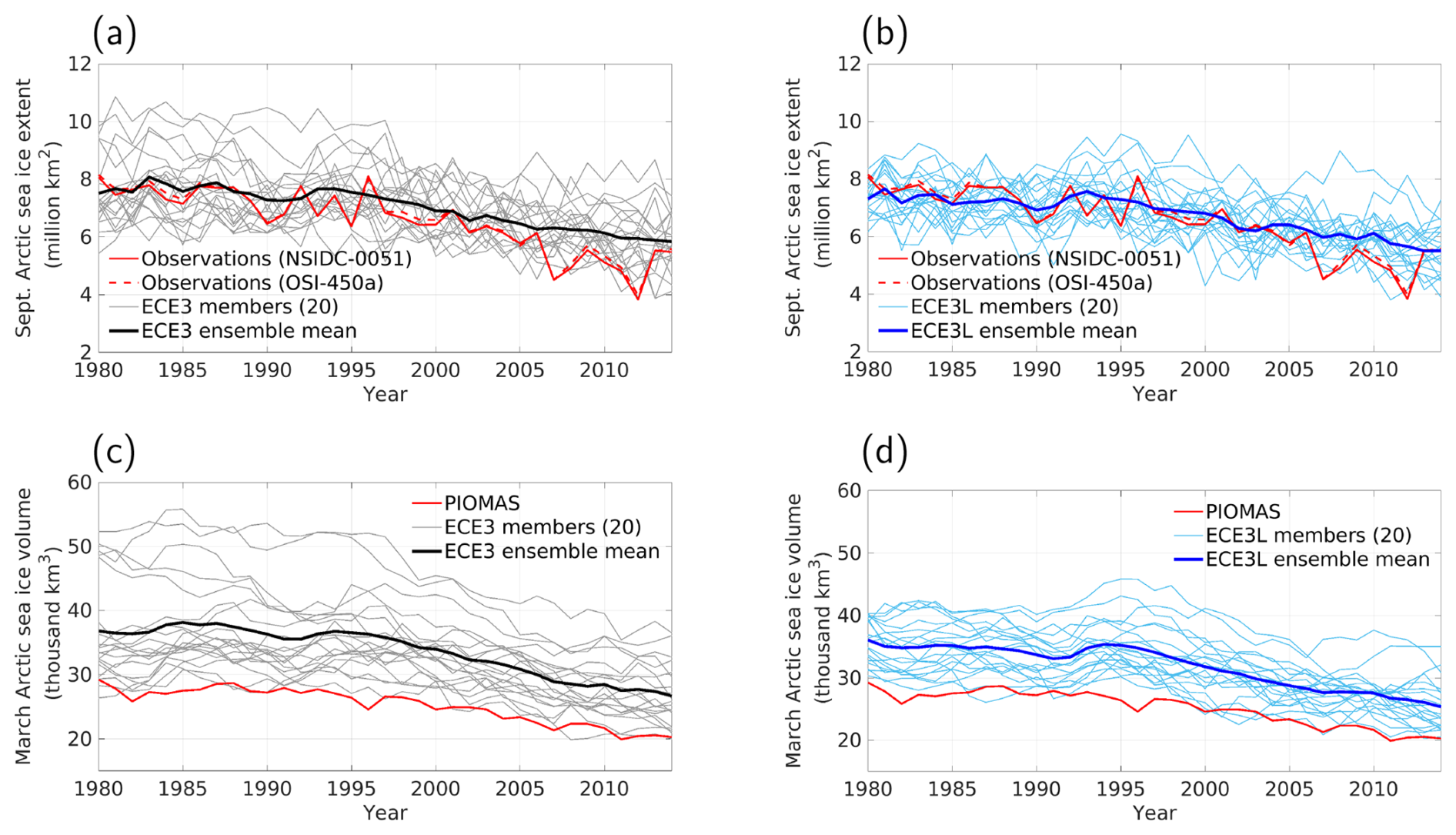
Figure 7 Arctic sea ice temporal evolution in the transient climate (1980–2014). Panel (a) presents the September extent (SIC>15 %) ensemble of ECE3. Panel (b) is the same as panel (a) but for ECE3L. Observations are from NSIDC with area pole-filling as well as OSI-450a. All datasets are remapped to the NSIDC-0051 grid. Panels (c) and (d) are the same as panels (a) and (b) but for the March volume (following the definition of the PIOMAS domain for areas thicker than 0.15 m).

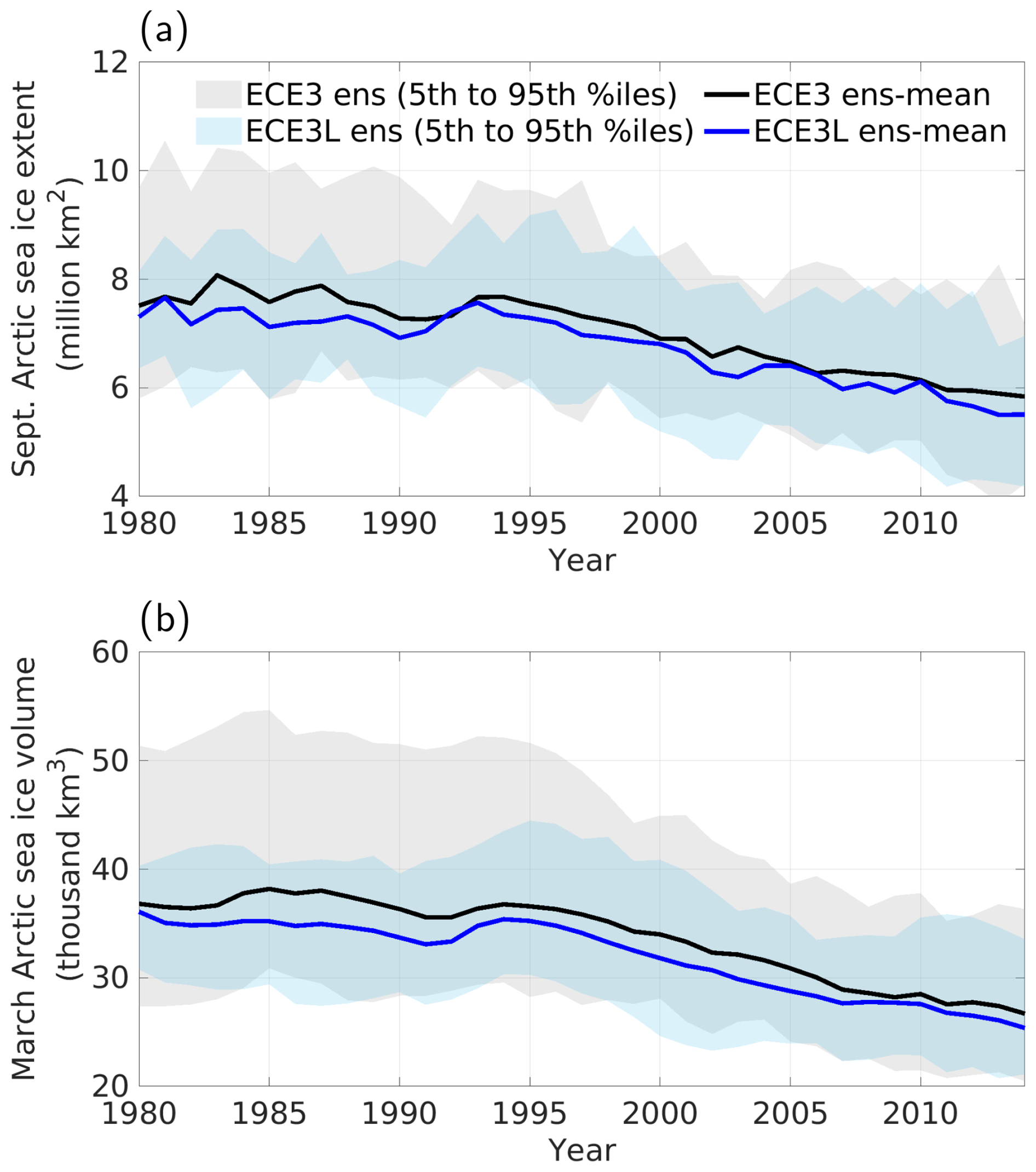
Figure 8 ECE3 and ECE3L Arctic sea ice (1980–2014). Panel (a) presents the September extent ensemble mean and the 5th to the 95th percentiles of 20 members, while panel (b) shows the March volume ensemble mean and the 5th to the 95th percentiles of 20 members. Ensemble mean differences are statistically significant (p<0.05, two-sided t test); however, after detrending, residuals for both models are not significantly different (p>0.05).

The model spread of ECE3 exhibits notable decadal changes before and after the 1990s in the transient climate, whereas ECE3L shows a relatively consistent and smaller spread across the same period (Figs. 7 and 8). This stability in ECE3L is accompanied by substantial reductions in overestimated sea ice area and volume prior to 1990, suggesting that incorporating the amplification effect through leads in the central pack ice refines the model's estimates of the declining sea ice volume trend overestimated in ECE3, at least to some extent. A supporting analysis (Fig. S5) shows that the initialized ECE3L ensemble recovers the internal variability in the Atlantic Meridional Overturning Circulation (AMOC) and global mean temperatures after a short spin-up, indicating that the smaller model spread in sea ice metrics is not an artefact of the initialization method but rather a result of reduced bias achieved through the new parameterization.

In this sensitivity study, the parameterization amplifies winter heat loss to reduce ice thickness and dampens summer heat uptake to delay melt, potentially addressing seasonal biases such as excessive winter ice thickness and premature summer melting, which would otherwise shift the annual minimum from September to August (Doescher et al., 2022; Keen et al., 2021). In ECE3, A_lead is most effective in colder conditions with excessive sea ice, where greater sea ice coverage and atmospheric stability contribute to large model variability before 1990 (Fig. 7). However, as the Arctic warms, its influence weakens due to reduced winter stratification and continued summer sea ice retreat (Deser et al., 2010). Consequently, its impact on mitigating summer sea ice bias remains limited. Thus, the smaller spread in ECE3L is a direct result of bias reduction in sea ice representation rather than an artificial constraint on variability.

4.2 Enhanced performance: reduced regional bias and improved representation of the sea ice edge

Arctic sea ice thickness fields reveal the impacts of heat flux modulation during the March maximum and September minimum periods (Fig. 9). Ensemble mean comparisons show that, in March, the mean SIT in the central Arctic for ECE3L in the transient climate generally exceeds 3 m, greater than the 30-year mean of ExpCold (Figs. 3a and 9a). The reduction in SIT between ECE3L and ECE3 (i.e. thinning of central pack ice where SIC≥70 %) is also lower in the transient climate than in ExpCold (Figs. 3b and 9b). Similarly, in September, the central Arctic SIT for ECE3L in the transient climate remains greater than in ExpCold, with changes (ECE3L minus ECE3) again being more pronounced in ExpCold (Figs. S3a and b and 9c and d). Notably, in ECE3, the mean SIT in March is slightly higher in the central Arctic in ExpCold than in the transient climate, with minimal differences observed in summer (not shown). The generally thicker ice in ECE3L in the transient climate is due to the diminished effect of heat flux amplification on ice thinning, compared to the more pronounced effect in ExpCold.

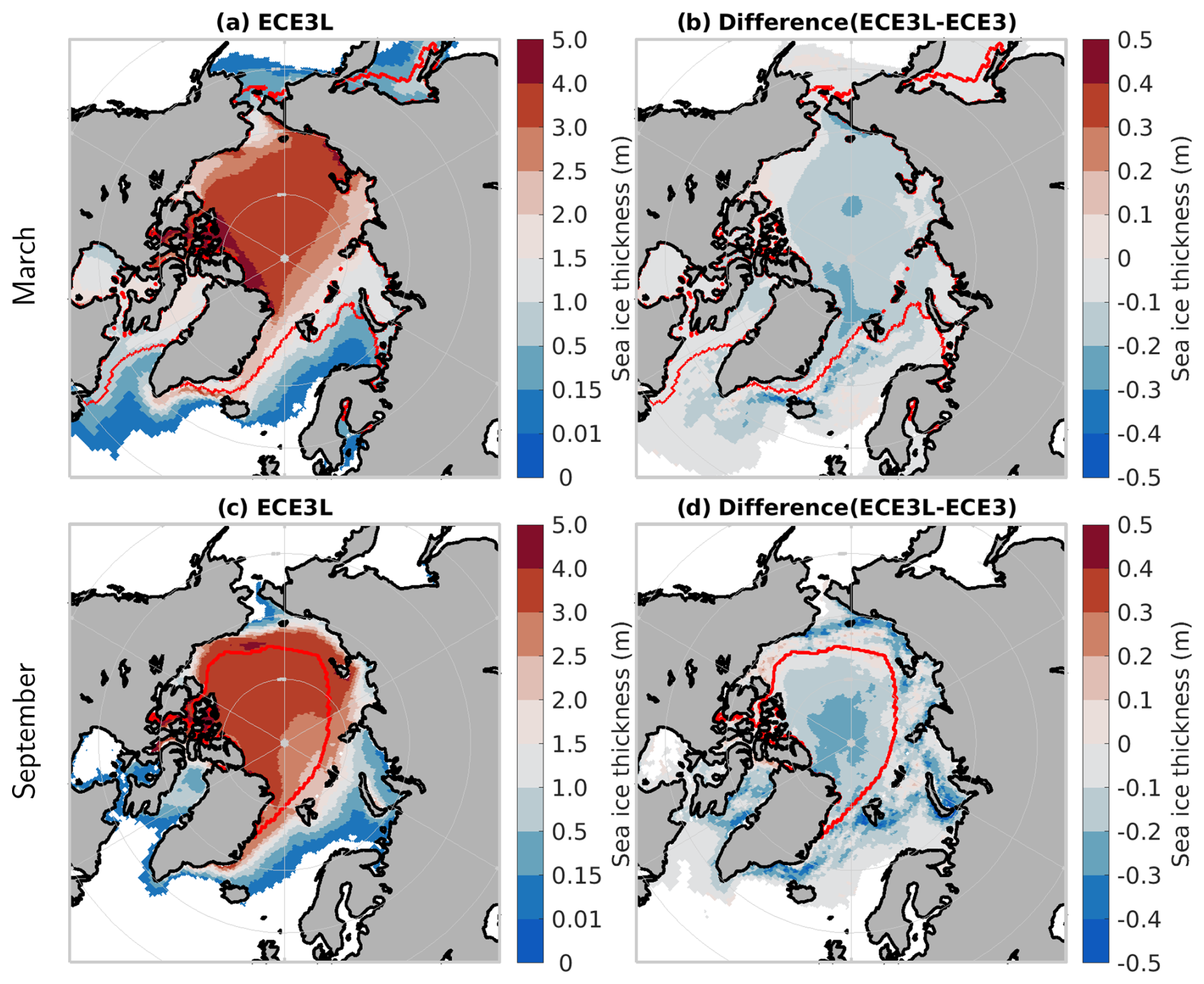
Figure 9 Ensemble mean Arctic maps (1980–2014) for the (a) ECE3L March sea ice thickness and (b) ECE3L minus ECE3 difference. Panels (c) and (d) are the same as panels (a) and (b) but for September. Note that a nonlinear colour scale is used in panels (a) and (c) to emphasize low ice thicknesses. Thicknesses under 0.01 m are not shown. Note that the PIOMAS domain is defined as SIT>0.15 m (see colour bar). The areas with SIC≥70 % in both ECE3 and ECE3L are encompassed by red lines.

The Arctic sea ice concentration maps for March and September climatologies in both ensemble means (Fig. S6) closely resemble those observed in the mean states for ExpCold (Figs. 4a and b and S4a and b), although with moderate differences between ECE3L and ECE3. To accurately assess these models, we employ the integrated ice-edge error (IIEE) metric with a 15 % threshold for the sea ice edge (Goessling et al., 2016) and then compare the results with satellite observations from NSIDC (Fig. 10). As documented by Doescher et al. (2022), in March, ECE3 tends to overestimate the ice concentration near the ice margins in the Atlantic sector, whereas it underestimating the ice concentration in the Bering Sea and Sea of Okhotsk (denoted in Fig. 10d). ECE3L shows a notable improvement in reducing the positive bias found in the Atlantic sector, although it slightly increases the negative bias in the Pacific sector, noted in the Sea of Okhotsk. In September, ECE3 generally overestimates the sea ice concentration at ice margins, except in the Kara Sea, where it is underestimated. The improvement by ECE3L is particularly noticeable in the Atlantic sector. These findings are corroborated by an alternative satellite dataset (OSI-450a; not shown), aligning with Doescher et al. (2022). The monthly IIEE time series indicate that ECE3L consistently outperforms ECE3 across all months (not shown), with Fig. 11 illustrating significant differences in IIEE for March and September (p<0.05), as examples, and no detected trend over time. Notably, the model spread of ECE3, especially in winter months, has dramatically decreased since the 2000s. In contrast, the model spread of ECE3L has remained relatively low, with no apparent decadal shifts.

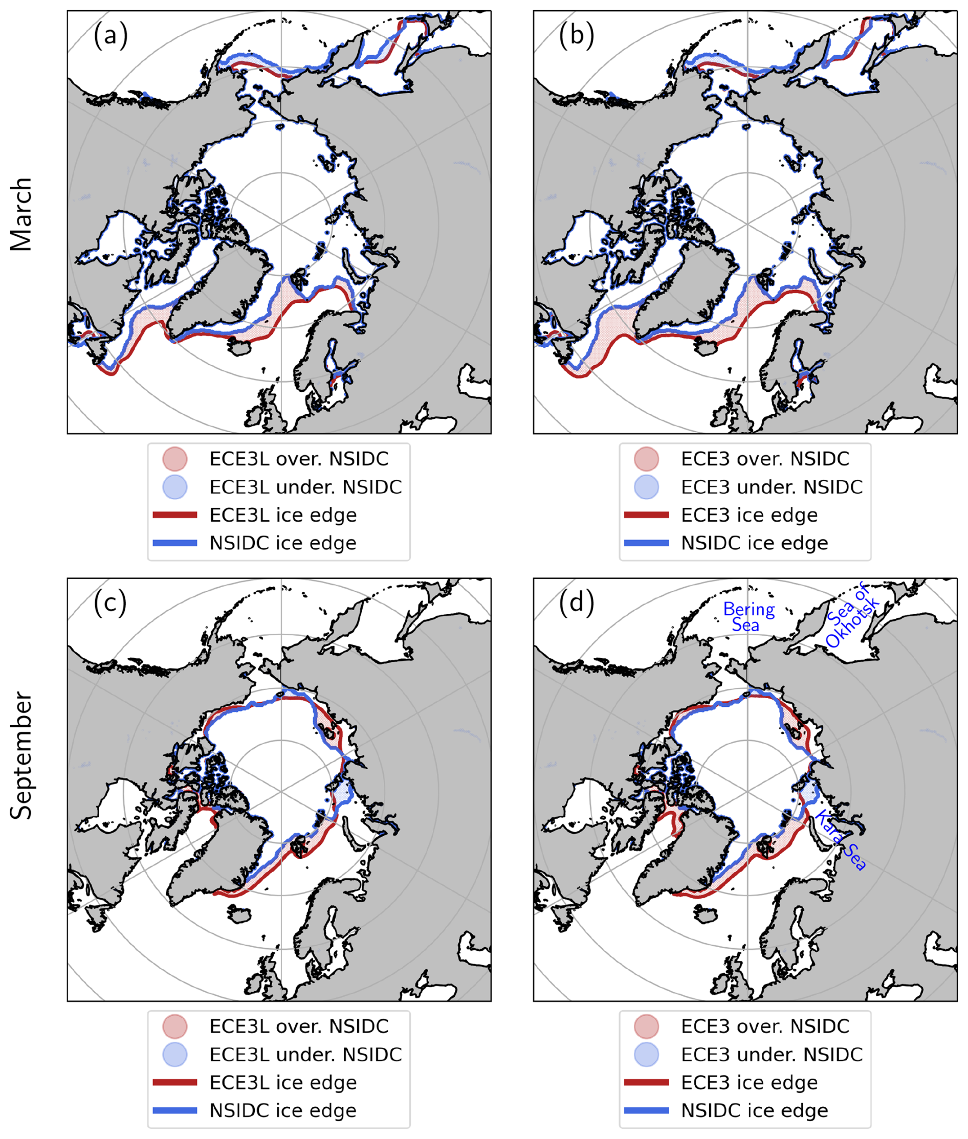
Figure 10 The integrated ice-edge error (IIEE; defined in Sect. 2.4) maps of ECE3L (a) and ECE3 (b) vs. NSIDC-0051 for the March sea ice climatology (1980–2014). Red and blue indicate whether the model's ensemble mean overestimates or underestimates the ice edge prescribed by NSIDC-0051, respectively. Panels (c) and (d) are the same as panels (a) and (b) but for September sea ice. The sea ice edge is defined by the 15 % sea ice concentration contour.

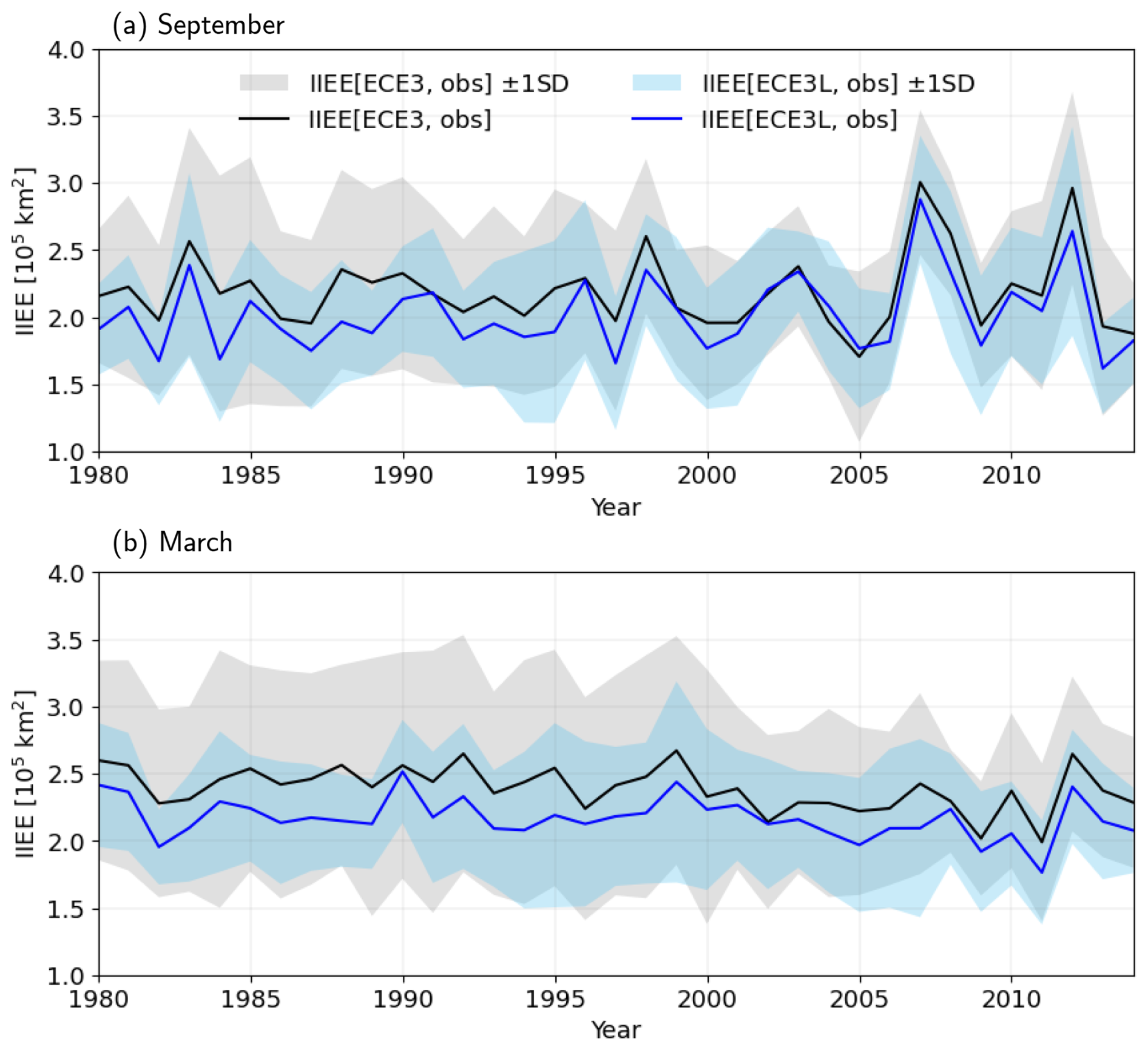
Figure 11 The temporal evolution of the integrated ice-edge error (IIEE) for September (a) and March (b) estimated for ECE3 (black) and ECE3L (blue) relative to NSIDC-0051 during the 1980–2014 period, with the ensemble means (thick line) and the model spread (the shaded area) indicated as 1 standard deviation from the mean across 20 members. The sea ice edge is defined by the 15 % sea ice concentration contour. Ensemble mean differences are statistically significant (p<0.05, two-sided t test); no trends are detected over time.

In summary, the annual climatologies for the changing sea ice conditions in the transient climate, as represented by the ECE3 and ECE3L ensemble means (Fig. 6), closely match those of the repeated climate scenario for ExpCold (Fig. 2). For the 1980–2014 period, the sea ice area and volume were 10.4×10⁶ km² and 27.6×10³ km³, respectively, representing a 3 % and 7 % reduction compared to ExpCold, with a sea ice area and volume of 10.9×10⁶ km² and 29.3×10³ km³, respectively, showing reductions of 12 % and 27 %. Notably, the mean sea ice thickness (defined as SIV divided by SIA) under both climate conditions for ECE3 is 2.7 m, yet the reductions in area and volume by ECE3L (relative to ECE3) are nearly 4 times larger under the repeated forcing of ExpCold than under transient historical forcing. This underscores the diminishing influence of sea ice leads on modifying the Arctic climate, largely due to the decreased occurrence of stable stratification in the winter as the Arctic warms.

5 Discussion

5.1 Implication of the differing sea ice evolution for Arctic warming

This study provides valuable insights for Arctic climate modelling. By incorporating a modulating factor for surface sensible heat flux over sea ice to account for processes over leads, the EC-Earth3 model shows closer agreement with the observed Arctic sea ice extent and volume, particularly under colder climate conditions. This adjustment mitigates a known bias in earlier simulations. Such developments offer a step forward in understanding the Arctic's response to climate change, with the potential to enhance the reliability and predictive capabilities of global climate models. Recent research emphasizes the importance of accurately representing sea ice processes to capture the complex feedback mechanisms that drive Arctic amplification and impact global climate patterns (AMAP, 2021; Docquier and Koenigk, 2021; Kay et al., 2022). The parameterization introduced in this study supports these insights, emphasizing the need to represent finer-scale ocean–sea ice–atmosphere coupling processes.

Focusing on surface warming, a primary indicator of climatic impacts, this section evaluates the differing impacts of sea ice evolution modelled by ECE3 and ECE3L on climate change. Specifically, it explores how these variations affect regional warming patterns, thereby enhancing our understanding of both the localized and broader implications of Arctic warming. Given the challenges in accurately measuring absolute T2m in the Arctic and globally (Rantanen et al., 2022; Tian et al., 2024), it remains uncertain whether ECE3L provides a better representation of the mean state and the warming trend. To address this, we computed the average of four observational or reanalysis datasets as reference fields, aiming to reduce warm-bias artefacts over Arctic sea ice in reanalyses under very cold conditions (Tian et al., 2024). As no differences were found in global mean temperatures between the ECE3 and ECE3L ensemble means, our subsequent analysis focuses on temperature trend maps to infer the local amplification ratio relative to the global warming rate. The temperature trend maps for 1980–2014 (Fig. 12a–c) show that ECE3L more closely aligns with observed trends along the ice edge in the North Atlantic sector of the Arctic compared to ECE3, which overestimates the warming trend in the Barents Sea, while underestimating it in the Greenland and Labrador seas. Additionally, ECE3L represents the warming trend in the East Siberian Sea, unlike ECE3, which consistently underestimates the trend in the Pacific sector of the Arctic (specific locations given in Fig. S1d).

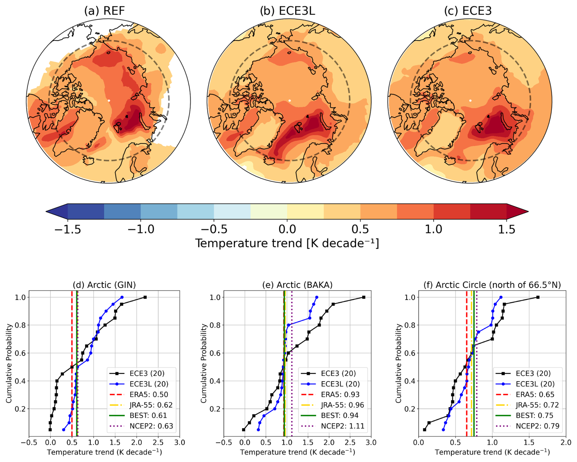
Figure 12 (a–c) Annual mean temperature trends for the transient climate (1980–2014), derived from the average of the observational datasets, ECE3L and ECE3. Areas without statistical significance are masked in panel (a), whereas panels (b) and (c) display significant trends across all areas. (d–f) Cumulative probability plots of the temperature trend from the ECE3 (black) and ECE3L (blue) ensembles for three regions: (d) the Greenland–Iceland–Norwegian (GIN) seas (40° W–15° E, 66.5–82° N), (e) the Barents and Kara (BAKA) seas (15–100° E, 70–82° N), and (f) the Arctic Circle. The locations of the GIN and BAKA regions are shown in Fig. 1c. The dashed grey lines in panels (a)–(c) depict the Arctic Circle (66.5° N latitude). Observations are from ERA5, BEST, JRA-55, and NCEP2.

The cumulative distribution function (CDF) analysis in Fig. 12d–f emphasizes regional differences in ensemble performance, with ECE3L exhibiting reduced variability and a central tendency that aligns more closely with observations than ECE3. This results in a more consistent representation of warming trends across the Greenland–Iceland–Norwegian (GIN) seas, the Barents and Kara (BAKA) seas, and the broader Arctic. Consequently, ECE3L achieves closer alignment with observed local amplification ratios (the ratio of local warming to global mean warming; Rantanen et al., 2022), leading to more confined estimates of Arctic amplification.

Constraining ensemble variability, which may incidentally improve certain forecast scores (Peterson et al., 2022), is not our objective. Instead, we aim to assess how the missing representation of heat flux over leads influences Arctic climate simulations. The narrower spread in ECE3L arises from the amplification effect of A_lead on surface heat exchange, rather than from deliberate tuning. This underscores the sensitivity of sea ice states to sub-grid-scale heat flux processes, highlighting the need for further investigation.

5.2 Advances and limitations

Current climate models often exhibit significant seasonal biases in sea ice simulations, which compromise the accuracy of long-term climate projections for the Arctic (Doescher et al., 2022; Keen et al., 2021). Studies by Deser et al. (2010) and Frankignoul and Kwonb (2024) highlight how misrepresentations of critical feedback mechanisms, such as the ice–albedo feedback, can lead to inaccuracies in seasonal sea ice predictions. This feedback is crucial in Arctic amplification, where retreating sea ice results in more open water, which absorbs more solar radiation, further warming the region and exacerbating sea ice melt in a cycle that accelerates the decline of Arctic sea ice. These biases not only impact the Arctic atmospheric stability but also influence seasonal atmospheric and oceanic circulations (Frankignoul and Kwonb, 2024).

To improve the accuracy of seasonal predictions and climate projections for the Arctic, it is essential to account for unresolved oceanic and atmospheric coupling processes (Eyring et al., 2021; Docquier and Koenigk, 2021). Turbulent heat exchanges over leads, which affect Arctic climate dynamics, require finer-scale process parameterization due to their fractal nature, spanning from metres to kilometres (Marcq and Weiss, 2012; Esau, 2007). This fractal complexity introduces uncertainty, particularly related to the properties of sea ice floes, such as the thickness, damage, and age, which remain poorly quantified. Addressing this gap, Davy and Gao (2019) introduced a fixed fractal dimension derived from satellite observations. Recent studies using large-eddy simulations (LESs) have further underscored that the lead width, background wind, and surrounding ice roughness can strongly influence heat flux (Gryschka et al., 2023), suggesting that reducing the structural uncertainties in models will require new, high-resolution data sources, like drone-based measurements.

The present study builds on this foundation by performing a sensitivity analysis focused on sensible heat flux, avoiding assumptions about the latent heat flux response to leads due to the absence of data from the original LESs of Esau (2007). Using the heat flux modulation factor developed by Davy and Gao (2019), in which the scale sensitivity is derived from the model results of Esau (2007), we incorporated this approach directly into a coupled climate model, a topic that has not been extensively explored in previous studies (Davy and Gao, 2019). This modification enhances the model's sensitivity to local sea ice and atmospheric conditions, improving Arctic sea ice simulations. Notably, our comparative analysis shows that ECE3L aligns more closely with the PIOMAS and NSIDC datasets (Schweiger et al., 2011; Stroeve et al., 2014) and reduces the model spread, particularly under conditions of thicker ice in the central Arctic and stronger winter atmospheric stability. Moreover, while our modifications influence Arctic conditions, they show limited global implications, consistent with the findings of Kay et al. (2022), thereby highlighting the potential for refining predictions of sea ice dynamics and their climatic impacts.

Despite these advancements in modelling the Arctic climate, significant challenges remain. Current models, including EC-Earth3, often struggle to capture the accelerated loss of Arctic sea ice that has been observed since the late 1990s (Lee et al., 2023). The mean state of sea ice, especially its thickness, is crucial for activating key feedback mechanisms that enhance model sensitivity to external forcing (Massonnet et al., 2018; Wunderling et al., 2020). These feedbacks are vital for reliably predicting the timing and implications of an ice-free summer in the Arctic Ocean. Additionally, ECE3L consistently overestimates sea ice volume up to the end of the analysis period, with the influence of sea ice leads expected to diminish in future climate simulations due to the decreasing coverage of thick ice and weakening winter stratification. Moreover, the new scheme does not fully recover the observed September minimum, underscoring persistent challenges in simulating late-summer sea ice loss. This limitation stems from its focus on atmosphere–ice heat flux modification, without directly addressing ocean–ice dynamics, which are crucial for accurately capturing summer retreat (Docquier and Koenigk, 2021). Addressing these deficiencies requires further research, particularly into how variations in sea ice and snow thickness affect heat and energy exchanges in the Arctic (Landrum and Holland, 2022). It is also essential to investigate how different representations of these processes can alter climate model sensitivity to external forcing (Webster et al., 2018).

Furthermore, this study relies on specific model configurations and parameterizations, which may not be directly applicable across different climate models. As indicated by Chen et al. (2023), significant inter-model spread in Arctic sea ice thickness within CMIP6 simulations compared to PIOMAS data highlight the need for broader application tests. Exploring the adaptability of the modulating factor approach across different models could help validate and generalize the findings, ultimately enhancing global climate projections.

The modulation factor A_lead is applied globally, including in the Antarctic. However, its local effect is confined to sea ice in the Weddell Sea and Ross Sea in ECE3L (not shown), due to a substantial warm bias in the Southern Ocean and the resulting underestimation of Antarctic sea ice, as identified in the ECE3 CMIP6 historical simulations (see Figs. 10 and 14 of Doescher et al., 2022). This diminishes the effect of parameterization in the Antarctic. Further refining parameterization to account for thinner sea ice in both the Antarctic and warming Arctic could provide insights into the contrasting behaviours and feedback mechanisms of sea ice, enhancing our understanding of polar climate interactions and potentially improving the accuracy of global climate projections.

6 Conclusions

This study explored whether and how the persistent positive bias in Arctic sea ice simulated within the global climate model EC-Earth3 can be alleviated in different climates by introducing a modulating factor, which adjusts surface sensible heat flux through leads in the central pack ice. Our evaluation, involving two sets of 50-year simulations and comparisons with two historical ensembles, demonstrates that the lead parameterization (ECE3L) significantly influence winter surface air temperatures in the Arctic, while having minimal impact on non-polar regions.

The spatial patterns in mean sea ice changes from 1980 to 2014 in ECE3L closely mirror those simulated using 1985 forcing (cold climate). However, the reduction in total Arctic sea ice area and volume is nearly 4 times greater in the cold climate, a period characterized by stronger atmospheric stability. This suggests that while the impact of amplified heat flux through leads is less effective under warming conditions, it remains crucial in colder climates, where ice loss and surface warming are more pronounced. As a result, this parameterization does not accelerate the transition to a warmer Arctic with less perennial sea ice; instead, it refines the long-term trends in sea ice volume decline and Arctic warming overestimated in ECE3. ECE3L shows reduced ensemble variability, leading to enhanced sea ice sensitivity to Arctic warming and providing more constrained estimates of Arctic amplification. Improved agreement with observational and reanalysis data, particularly in the North Atlantic marginal ice zone, emphasizes the critical role of atmospheric stability in shaping both sea ice states and the broader patterns of Arctic amplification.

In a warmer climate, the modulating factor can either increase or decrease sea ice states depending on prevailing atmospheric stability and the mean sea ice thickness, making the overall effects minimal and uncertain. This underscores the importance of accurately simulating sea ice dynamics to better understand the Arctic climate response to forcing. The next step is to refine the parameterization to include an ice-thickness-dependent modulation factor, effectively incorporating both Antarctic and Arctic sea ice simulations in a warming climate. This will help explore their broader implications for global climate projections.

Appendix A: Parameterization of surface heat flux over sea ice leads in a climate model

A1 Empirical relationship between the lead width and surface sensible heat flux amplification

Initially Esau (2007) established an empirical relationship between the lead width and sensible heat flux, quantified as an amplification effect, measuring the extra flux from leads compared to open water with the same air–sea temperature differences, using large-eddy simulations (LESs). Leads on the scale of a few kilometres in width produced the strongest amplification, aligning well with observed data (Fig. A1a) and contrasting with previous assumptions that narrow leads (1–25 m) yield the highest flux per unit area (Marcq and Weiss, 2012). This underscores the need to include 3D turbulence effects in parameterizing complex small-scale heat flux processes.

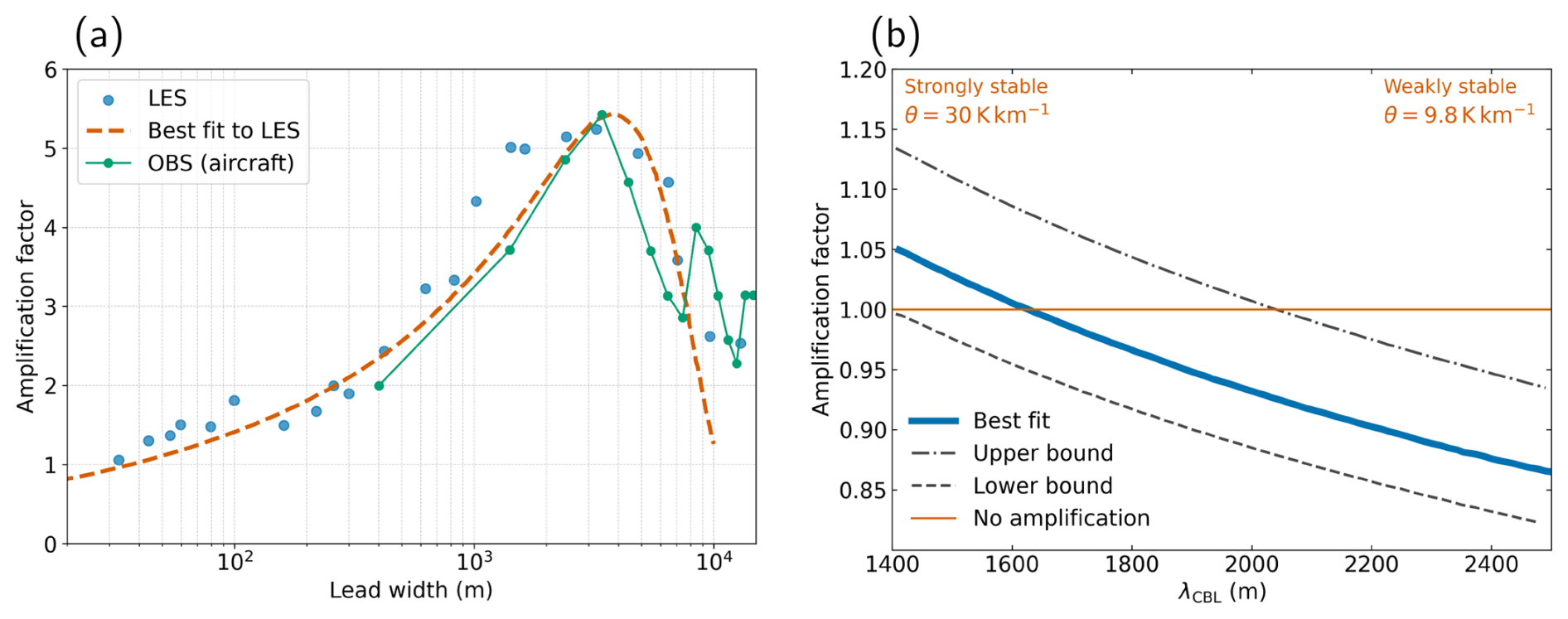
Figure A1 (a) The heat flux amplification factor (relative to open water) as a function of lead width, adapted from Esau (2007). Blue dots represent individual LESs, the dashed red line shows the best fit to LES data, and green dots indicate aircraft observations over the Baltic Sea. (b) The total sensible heat flux amplification across all leads. Panels (a) and (b) are adopted from Figs. 1 and 4 in Davy and Gao (2019), respectively.

Readers are encouraged to refer to Esau (2007), particularly Tables 1 and 2 and Fig. 4 in that publication, which detail how the amplification effect varies with atmospheric stability, defined by the convective boundary layer length scale (λ_CBL in metres), and lead width (x in metres). The best fit to two sets of LES results for weakly stratified (θ=9.7 K km⁻¹, λ_CBL=2500 m) and strongly stratified (θ=30.7 K km⁻¹, λ_CBL=1400 m) conditions is given in Eq. (A1).

$$\begin{array}{}\text{(A1)}& {\displaystyle }{\displaystyle }A\left(x\right)=\mathrm{5}{\left({\displaystyle \frac{x}{{\mathit{\lambda }}_{\text{CBL}}}}\right)}^{\frac{\mathrm{1}}{\mathrm{3}}}\exp \left({\displaystyle \frac{-{\left(\frac{x}{{\mathit{\lambda }}_{\text{CBL}}}-\mathrm{1}\right)}^{\mathrm{2}}}{\mathrm{4.84}}}\right)\end{array}$$

Here, A(x) represents the amplification factor, indicating how much greater the sensible heat flux per unit area is from the lead compared to open water.

A2 The lead width distribution from satellite observations

Satellite observations suggest that the lead width follows a power-law distribution with a negative exponent, indicating that narrow leads are most common (Marcq and Weiss, 2012, their Eq. 11).

$$\begin{array}{}\text{(A2)}& {\displaystyle }{\displaystyle }P\left(x\right)={\displaystyle \frac{a-\mathrm{1}}{L_{\mathrm{0}}}}{\left({\displaystyle \frac{x}{L_{\mathrm{0}}}}\right)}^{-a}\end{array}$$

Here, P represents the probability of finding a lead of width (x in metres), with L₀ (10 m) as the lower bound, determined by satellite resolution. The exponent a (where a>1) characterizes the steepness of the distribution. For more details, see Marcq and Weiss (2012), particularly their Figs. 2–4.

Marcq and Weiss (2012) applied two luminosity thresholds to distinguish leads from ice, producing two sets of power-law coefficients. As neither threshold is objectively preferable, Davy and Gao (2019) averaged these estimates, accounting for uncertainty to evaluate the total, large-scale effect of leads on the surface energy balance. The best estimates for a are 2.2 (low threshold) and 2.55 (high threshold).

A3 Integrating the lead width distribution for the total amplification factor

Davy and Gao (2019) calculated a total amplification factor for a grid cell with mixed ice and open water, assuming that the open water results from leads following the observed power-law distribution. This was done by integrating the product of the lead width probability distribution and the LES-derived amplification factor, as shown in Eq. (A3).

$$\begin{array}{}\text{(A3)}& {\displaystyle }{\displaystyle }\widehat{A}=\underset{L_{\mathrm{0}}}{\overset{\mathrm{\infty }}{\int }}A\left(x\right)P\left(x\right)\mathrm{d}x\end{array}$$

Here, $\widehat{A}$ represents the total amplification of sensible heat flux from leads within the grid cell, compared to that from an equal area of open water, and A(x) and P(x) are defined in Eqs. (A1) and (A2), respectively.

This equation requires a numerical solver to calculate the total amplification factor over a range of λ_CBL, based on LESs from Esau (2007) that cover conditions from strong stability (θ=30.7 K km⁻¹) to weak stability (θ=9.7 K km⁻¹). The results, shown in Fig. A1b, are best fit by an empirical relation between the maximum total amplification factor A_max and λ_CBL, as expressed in Eq. (A4).

$$\begin{array}{}\text{(A4)}& {\displaystyle }{\displaystyle }{A}_{\text{max}}=c_{\mathrm{1}}\cdot {\mathit{\lambda }}_{\text{CBL}}^{\mathrm{2}}-c_{\mathrm{2}}\cdot {\mathit{\lambda }}_{\text{CBL}}+c_{\mathrm{3}},\text{ if SIC}\ge \mathrm{90}\mathrm{\%}\end{array}$$

Here, $c_{\mathrm{1}}=\mathrm{6.012}\times {\mathrm{10}}^{-\mathrm{8}}$, $c_{\mathrm{2}}=-\mathrm{4.036}\times {\mathrm{10}}^{-\mathrm{4}}$, and c₃=1.56, with a cap of [0.8, 1.2].

The effective factor A_lead is linearly interpolated between 1 and A_max, as defined in Eq. (A5).

$$\begin{array}{ll}{\displaystyle }{A}_{\text{lead}}=& {\displaystyle }\mathrm{1}+(A_{\text{max}}-\mathrm{1})\cdot {\displaystyle \frac{max(\mathrm{0},\text{SIC}-\mathrm{70})}{\mathrm{90}-\mathrm{70}}},\\ \text{(A5)}& {\displaystyle }& {\displaystyle }\text{ if SIC}<\mathrm{90}\mathrm{\%}\end{array}$$

When the fraction of open water exceeds 30 % (i.e. SIC≤70 %), A_lead becomes a constant value of 1.

A4 Implementation to the EC-Earth3 model

The depth of the convective boundary layer (λ_CBL in metres) is determined using Eq. (A6), where the key parameter $\mathit{\theta }=\frac{\mathrm{d}T}{\mathrm{d}z}$ (in  K m⁻¹) characterizes the atmospheric stability at a height of between 200 and 300 m, depending on the vertical resolution of the atmospheric model (Davy and Gao, 2019). In the EC-Earth3 model configuration, temperature changes (ΔT, in K) between model levels 86 and 91, which correspond to approximate heights of 200–250 m from the Earth's surface, are used. The empirical expression in Eq. (A6) is conveniently expressed using ΔT with constant values of $\widehat{c_{\mathrm{4}}}=\mathrm{230}$ m K⁻¹ and c₅=2100 m, so that the resulting λ_CBL typically ranges from 1400 to 2500 m. This range was derived from the LESs, which were tested under conditions from strongly stable stratification (30.7 K km⁻¹) to weak stratification (9.7 K km⁻¹). No more strongly stable stratification was observed in the lowest model level. The constants c₄ and c₅ were adjusted based on the temperature changes between the specified model levels in the EC-Earth3 model configuration. These values were chosen to be consistent with the results of the original LESs of Esau (2007), and they will be different if different model levels or atmospheric models are employed.

$$\begin{array}{}\text{(A6)}& {\displaystyle }{\displaystyle }{\mathit{\lambda }}_{\text{CBL}}=c_{\mathrm{4}}{\displaystyle \frac{\mathrm{d}T}{\mathrm{d}z}}+c_{\mathrm{5}}=\widehat{c_{\mathrm{4}}}\cdot \mathrm{\Delta }T+c_{\mathrm{5}}\end{array}$$

Figure S1 shows examples of A_lead for ExpCold and ExpWarm in the Arctic, respectively. This calculation is based on the lapse rate and sea ice concentration from previous atmosphere-only (AGCM) simulations in the Blue-Action project with EC-Earth3 (Liang et al., 2020). The AGCM simulations were forced by the historical forcing of CMIP6 and the surface boundary conditions from global daily $\mathrm{1}/\mathrm{4}$° SSTs and SICs from the UK Met Office Hadley Centre Sea Ice and Sea Surface Temperature dataset (version 2.2.0.0; https://www.metoffice.gov.uk/hadobs/hadisst2/, last access: 21 July 2025, Titchner and Rayner, 2014.) The modulation effects exhibit remarkable seasonal variation, influenced by the background atmospheric stability, in the Arctic regions (see Fig. S1). During the winter months, there is an additional heat flux from the warm ocean through the leads to the atmosphere by means of the modulating factor above 1. In contrast, during the summer months, the surface heat flux through the leads is reduced because the modulating factor is below 1. The areas where the lead parameterization takes effect (SIC>70 %) and ice cover is thicker than 2 m have experienced substantial reductions from ExpCold to ExpWarm, particularly in the summer (as seen in Fig. S1b and d). This suggests that the sea ice state, along with the presence of leads, has undergone significant changes during this period. These seasonal and interannual variations in the impact of leads on heat flux through the sea ice play a crucial role in the dynamics of the Arctic regions and their response to changing climate conditions.