Aspect controls on the spatial redistribution of snow water equivalence through the lateral flow of liquid water in a subalpine catchment

Quantifying subalpine snowpack parameters as they vary through time with respect to aspect and position on slope is important for estimating the seasonal storage of snow water resources. Snow depth and density are dynamic parameters that change throughout the progression of the accumulation and melt periods, with direct implications on the distribution of snow water equivalence (SWE) across a landscape. Additionally, changes in density can infer physical processes occurring within the snowpack, such as compaction, liquid water ponding, and lateral flow. In this study, we measure snow depth and density throughout the Dry Lake watershed, a 0.25 km² watershed in northern Colorado, USA, using L-band (1.0 GHz) ground-penetrating radar (GPR) and coincident depth probing. We calibrated these surveys using snow pit observations and a SNOTEL station. A physical snowpack model, SNOWPACK, with inputs from a local remote automated weather station and a SNOTEL station produced simulations of snow depth, snow density, and liquid water content (LWC). The model simulations indicate mid-winter melt events produced LWC on the south aspect that is less present in the north aspect and flat areas. These mid-winter melt events, in combination with observations, are interpreted to result in the lateral flow of LWC downslope and the redistribution of SWE. Further observations show a steady increase in soil moisture in sensors at the SNOTEL station throughout the winter in the flat terrain and ice layer formation on the south aspect snow pits during mid-winter surveys. Other key observations include ponding of liquid water at the base of the north aspect during the later spring season melt phase evidenced by GPR transects. We further develop a perceptual model for the aspect controls on the distribution and movement of SWE during the winter and spring seasons. In summary, for the Dry Lake watershed mid-winter melt events are observed on south aspects and interpreted to cause a redistribution of SWE downslope, while spring melt brings liquid water ponding at the base of north aspects. These differences in snowmelt dynamics are based primarily on aspect, providing important processes to consider for spatially and temporally extensive SWE measurements moving forward.

1 Introduction

Accurately quantifying the spatial and temporal variability of snow water equivalence (SWE) can provide valuable insights for water resources. The variability of SWE can inform spring and summer streamflow generation (Li et al., 2017), soil moisture levels (McNamara et al., 2005), and groundwater recharge (Brooks et al., 2021). Additionally, the timing and quantity of runoff from snowmelt can help predict flooding, drought, streamflow volumes, and reservoir storage (Zeinivand and De Smedt, 2010; Modi et al., 2022; Bishay et al., 2023). SWE is commonly measured using weather station networks, like the SNOTEL network in the western United States, that utilize snow pillows, snow depth sensors, soil moisture, and precipitation gauges. However, these sites offer limited use in streamflow forecasting due to them being point measurements and forecast methods not accounting for deviation from climate stationarity (Sturm et al., 2017; Bales et al., 2006). Shifting global patterns in moisture delivery contribute to the increased importance in measuring SWE for snow-dominated catchments (Clow, 2010; Nolin et al., 2021). Thus, the expansion of snowpack monitoring is necessary to account for spatial and temporal variability found in mountainous environments (Painter et al., 2016; Fassnacht, 2021).

Snowpack properties are sensitive to energy balance dynamics, which is typically expressed in four phases: (1) the accumulation phase, (2) the warming phase in which the average snowpack temperature increases towards 0 °C, (3) the ripening phase in which phase changing occurs but liquid water is retained in the snowpack, and (4) the output phase where further inputs of energy cause melting to leave the snowpack as snowmelt output (Dingman, 2015). Terrain features like aspect can drastically alter the energy balance, especially in mid-latitude regions where sun incidence angle will preferentially expose south aspects to shortwave radiation during the day (Molotch and Meromy, 2014; Hinckley et al., 2014; Erickson et al., 2005). Canopy is another feature that can alter snowpack energy balance (Musselman et al., 2008; Webb, 2017). Canopies can prolong melt by shielding snow from shortwave radiation (Musselman et al., 2012; Varhola et al., 2010; Lundquist et al., 2013). Canopy will also influence the wind redistribution of snow, increasing the variability of snow accumulation and melt (McGrath et al., 2019; Webb et al., 2020b). Similarly, topography can influence wind sheltering and redistribution (Elder et al., 1991; Marks et al., 2002; Winstral et al., 2002). Once the snowpack melts, hillslope processes and soil texture will influence the hydrologic flow paths that form (Webb et al., 2018a; Hinckley et al., 2014; Jencso and McGlynn, 2011).

The snowmelt input for hydrologic response will rely on the spatiotemporal distribution of SWE, often collected through surveys. Snowpack properties such as bulk snow density are often assumed to be relatively uniform across landscapes based off storm accumulation patterns which can be predicted by air temperature (Valt et al., 2018). Snow density is commonly measured by massing a known volume of a cylinder or a triangular prism, which can be completed as a snow course survey with a federal sampler or with other tools in a snow pit (Kinar and Pomeroy, 2015). Additionally, dry-snow density can be derived from dielectric permittivity (Kovacs et al., 1995; Webb et al., 2021b), which measures the resistance of a medium to the formation of an electric field. Permittivity defines the velocity at which a radar wave will travel through a medium such as snow, allowing active radar systems to estimate bulk snow density. Permittivity may also be used to estimate bulk snow liquid water content (LWC), provided an estimate of dry-snow density or bulk density is available (Heilig et al., 2015; Koch et al., 2014; Mitterer et al., 2011; Schmid et al., 2015). Thus, ground-penetrating radar (GPR) can provide an opportunity to survey spatial patterns with high precision and control over survey locations. Additionally, emerging technologies such as L-band InSAR depend on knowledge concerning the variability of snowpack properties to constrain uncertainty and improve snow products (Tarricone et al., 2023).

Snowpack properties like snow depth and snow surface wetness are increasingly being surveyed using remote sensing techniques like airborne lidar, multispectral sensors, and synthetic aperture radar (SAR) (Currier et al., 2019; Painter et al., 2016; Skiles et al., 2018; Tarricone et al., 2023). These products often work best in tandem with one another to provide validation, introducing a strong argument for using multiple methods in assessing snowmelt. C-band SAR has been shown as capable of detecting snowmelt and complements snow cover products from Sentinel-2 (Guiot et al., 2023). However, the resolution of these products may be limited and unable to capture small-scale variability as it is influenced by terrain (Fassnacht et al., 2018). One example of higher-resolution data is products produced by the Airborne Snow Observatory (ASO) such as spectral albedo, SWE, and depth for basins using lidar and multispectral remote sensing platforms (Painter et al., 2016). These products are appropriate for understanding large-scale spatial patterns and resolutions as fine as 3 m; however, these data must rely on modeled snow densities to produce extensive SWE estimates and only represent a brief snapshot in time (Raleigh and Small, 2017). The use of ground-based survey techniques such as GPR allows surveys at intermediate spatial scales (between point-based stations and airborne platforms). When paired with precise measurements of snow depth (d_s), snow dielectric permittivity (ε) can be used to estimate snow density and liquid water content (Sommerfeld and Rocchio, 1993; Kovacs et al., 1995; Webb et al., 2018c; Bonnell et al., 2021; McGrath et al., 2022). Because the GPR signal is sensitive to properties such as snow density, GPR surveys enable the interpretation of snowpack properties as they relate to various physiographic controls (Webb, 2017; McGrath et al., 2019; Tarricone et al., 2023; Marshall and Koh, 2008; Bonnell et al., 2021; McGrath et al., 2022). For these reasons, GPR has been broadly used to observe ε to estimate snow properties (Marshall et al., 2005; Webb, 2017). GPR data can also be collected with minimal disturbance to the snowpack, unlike snow pits, is less time consuming, and d_s observations can be easily be gathered using a depth probe along the same survey track.

Therefore, to assess seasonal variability in the spatiotemporal distribution of SWE as it relates to energy balance dynamics, we employ L-band GPR technology to survey snow depth and density with respect to north and south aspect slopes and the relative position on each slope. We use these techniques to answer the following research question: how do variations in snowmelt dynamics impact snow density and SWE distribution throughout the snow season based on aspect and relative location on a hillslope? We aim to answer this question in a manner that will provide insights to snowmelt dynamics for mid-latitude forested mountains that develop a seasonally persistent snowpack.

2 Methods

2.1 Study site description

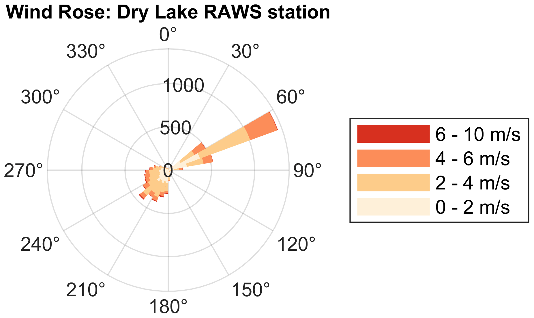
The study site for this research is in the Dry Lake watershed, a small watershed that is ideal for studying snow processes in northern Colorado, USA. The watershed is ∼ 0.25 km², with year-round, hourly data collection from a SNOTEL station and a remote automated weather station (RAWS) located within the extents of the watershed. Elevations range from 2500 to 2660 m above sea level (m a.s.l.), and the primary study area depicted in Fig. 1 has a mean elevation of 2545 m a.s.l. The SNOTEL station at the site measures a median peak SWE of approximately 510 mm occurring in early April (median date of 10 April from 1991–2020). Wind direction at Dry Lake is predominantly in the northeast to east direction (Appendix A), parallel to the contours of the north and south aspect hillslopes of the watershed.

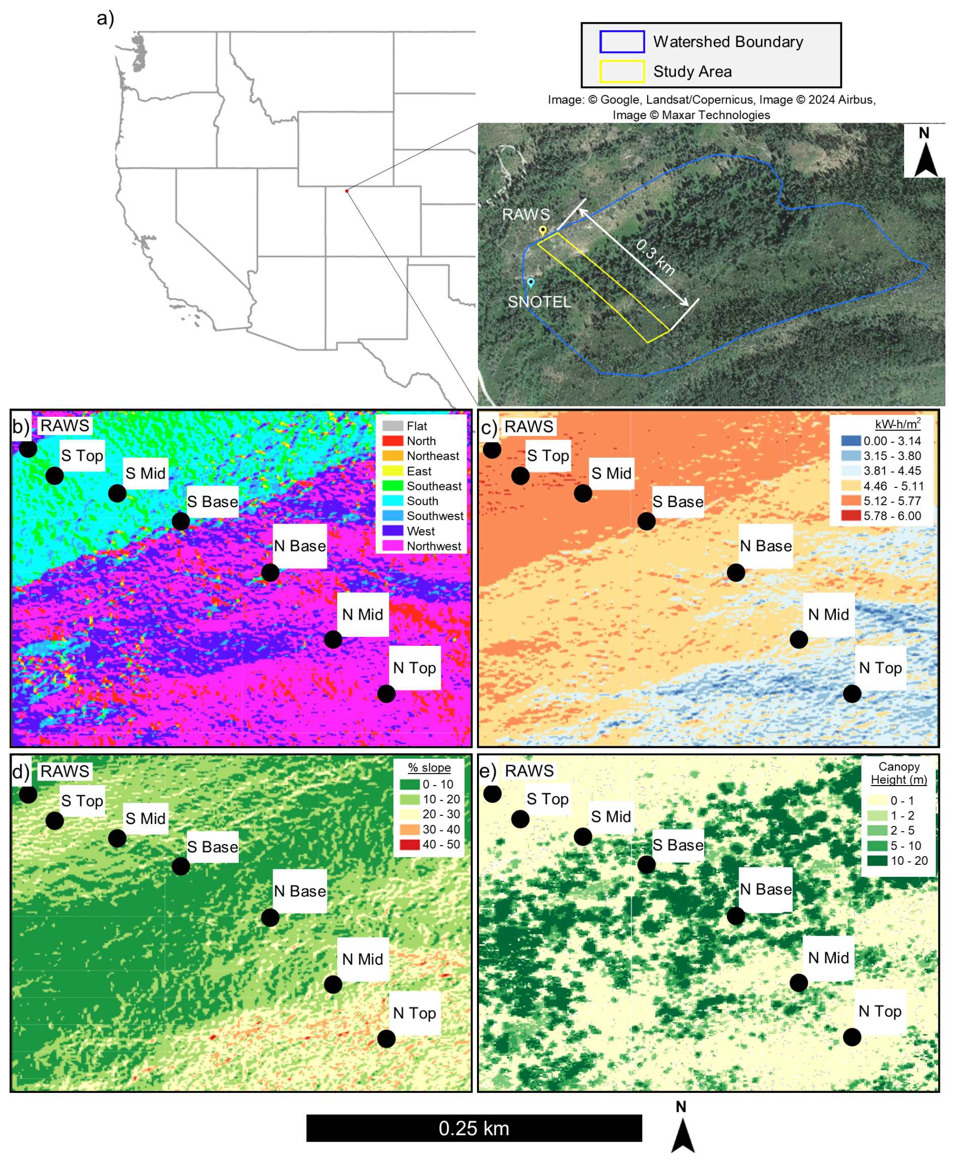
Figure 1 (a) The location and imagery of the Dry Lake watershed, including the general location within the western USA. (Imagery gathered via Google Earth Pro v. 7; Google Earth, 2024; © Google.) (b) Aspect map, (c) solar radiation model for 1 March, (d) percent slope of terrain, and (e) canopy height. Survey transect locations are indicated by black circles.

The soils in the Dry Lake watershed are loam on the flatter aspects, with observations of highly organic soils in the flat area at the base of the north aspect hillslope, cobbly sandy loam on the north aspect, and loam with very cobbly loam on the south aspect (Webb et al., 2018a). A layer of forest litter, or duff layer, also forms on the north aspect hillslope at a depth of approximately 8–15 cm, with depths up to 20 cm at the base of the slope. Depth to bedrock ranges from 0.12 m to greater than 1 m, with a mean depth to bedrock of 0.40 m. A small stream runs from the northeast to the southwest, with an outlet near the SNOTEL station. The lower area consists of mixed coniferous trees and is populated with ferns in the summer months, and the lower portion of the south aspect is populated by deciduous aspen canopy.

Lidar data were used to develop terrain and canopy height datasets to quantify the spatial variability of the site (Co, 2016). Using a 1 m digital elevation model (DEM), the flat terrain shares low-angle north- to west-facing surfaces and contains the tallest canopy height, resulting in moderate solar radiation (Fig. 1b). The north aspect consists of a mixture of north- to west-facing surfaces and the south aspect consists of primarily south- to southeast-facing surfaces. Solar radiation was calculated using the solar radiation tool in ArcGIS Pro for 1 March (Fig. 1c). The north aspect has medium to low solar radiation from terrain shading, and the highest solar radiation is seen on the south aspect hillslope. Also from the DEM, the north aspect is slightly steeper than the south aspect. A canopy height was also calculated (Fig. 1d), showing denser canopy at the base of the hillslopes, a shorter sparse canopy at the middle of the north aspect, and open canopy near the top of the north aspect. There is less canopy influence during winter months on the south aspect due to fewer trees and those trees being deciduous species.

2.2 Data collection

In the winter and spring of 2023 (12 January through 1 May), seven transects were established to collect data at varying positions on the flat, north, and south aspects. The spatial distribution of these transects was designed to capture changes in snow properties related to aspect and position on slope, including the base, middle, and top of slopes (Fig. 1). Transects were selected with minimal canopy influence with respect to shading and wind drifts. A flat terrain transect was taken by traversing a circle around the SNOTEL station, whereas all other transects were ∼ 20 m in length perpendicular to the fall line (i.e., parallel to slope contours). The base of the north aspect has some shading from coniferous canopy, though shading is predominantly from the terrain at this location, whereas the base of the south aspect has some slight shading from a deciduous canopy. These data were collected approximately once every month from January to May, resulting in five survey dates in 2023 (12 January, 6 February, 25 February, 1 April, and 1 May). All transects included GPR data collected with surface-coupled, common offset GPR units pulled over the snow. The first three surveys used a plastic sled to hold the GPR, whereas the GPR was pulled freely without a sled during the final two surveys. Both methods of towing were manually towed behind an individual on skis. Two GPR systems were used: a pulseEKKO GPR system for four of the surveys and a Mala Geosciences GPR system during one of the surveys due to the pulseEKKO being at another location at the time of survey. The pulseEKKO system used a shielded antenna at 1000 MHz. The Mala GPR system used a 1600 MHz antenna and was only used during the 25 February survey. Following the GPR, depth measurements were collected in the track of the GPR at 2 m spacing (Webb and Mooney, 2024a). Depending on the length of the transect, the number of depth measurements ranged from 8 to 30 measurements, with an average of 13 manually probed d_s measurements to average for each transect area (López-Moreno et al., 2011).

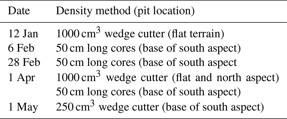
Snow pits were additionally dug to measure bulk density of the snowpack within the flat terrain, on the north aspect, and at the base of the south aspect (Webb and Mooney, 2024b). GPR transects were conducted next to the snow pits to calibrate GPR-derived density measurements for each survey date. When time allowed, 1000 cm³ wedge cutters were used to determine a density profile at 10 cm intervals. During days when time was limited, ∼ 50 cm long cores with diameter of ∼ 6.2 cm were used to estimate snow density. Thus, each snow pit had 2–20 measurements of density, depending on the time available for pit observations to derive bulk density. A table noting survey dates and density methods is available in Appendix B (Table B1). Notes were also taken about qualitative observations of liquid water ponding or ice lenses with depth of occurrence and approximate thickness.

2.3 Data processing

Radar data for each transect were processed using ReflexW, a software developed for near-surface geophysical data processing and interpretation. The first processing step was to apply a dewow filter, which removes low-frequency noise in the time domain by subtracting a running mean from the central point. Applying this filter allows the trace to have a mean of zero, which removes any slope in the trace and allows for positive and negative signals throughout the trace. A time-zero correction was applied next by selecting the first airwave break. A gain filter was then applied to account for signal attenuation and geometrical spreading loss as the wave propagates through the snow by amplifying the strength of later arrivals. An AGC-Gain function was used, which applies a multiplying factor to successive regions of the trace in time, dampening noise. The next step was to edit trace range along the x axis. This step can be used to remove time periods when the GPR was not moving. During data collection, there are periods of standstill between when the device is powered on and when the transect data are being collected, as well as between when the transect ends and when the device is turned off. Removing the traces before and after effectively crops the radargram to only include the transect data and not oversample the ends of the transect. Finally, a background removal filter is applied. This filter removes any excess noise and excess banding that may be present in the traces. In this step, the processing is set for all data at 1 ns or greater to retain the surface wave, which retains the clarity of the surface wave and soil–snow interface wave during picking. Next, the surface and soil–snow interface reflections were “picked” using a semi-automatic picking tool in ReflexW. Figure 2a displays an example of a radargram showing the snow surface reflection and snow–soil interface reflection. The surface wave reflection was then subtracted from the snow–soil interface reflection to determine the two-way-travel time (TWT) through the snow (Webb and Mooney, 2024c). Images of all radargrams are available in the Supplement (Figs. S1–S32).

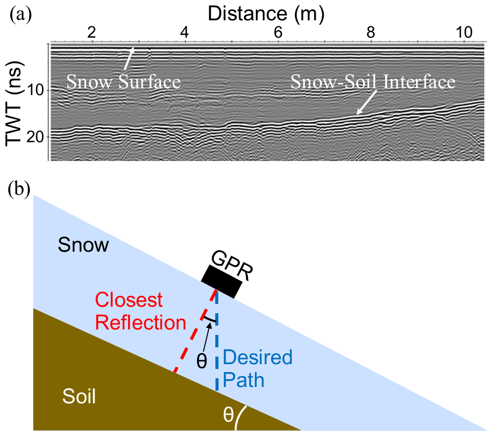
Figure 2 (a) An example of a processed radargram and the snow surface and snow–soil interface reflections. (b) A graphical depiction of the correction for slope angle to align TWT and depth probing for each transect.

The median TWT (ns) for each GPR transect and associated average measured d_s (m) were used for the following calculations to estimate bulk snowpack density by first calculating radar wave velocity (v),

$$\begin{array}{}\text{(1)}& v={\displaystyle \frac{d_{\mathrm{s}}}{\frac{\mathrm{TWT}}{\mathrm{2}}}},\end{array}$$

where v is in m ns⁻¹, and ε is calculated with the speed of light (c) in a vacuum,

$$\begin{array}{}\text{(2)}& \mathit{\epsilon }={\left({\displaystyle \frac{c}{v}}\right)}^{\mathrm{2}},\end{array}$$

and bulk density (ρ_s, kg m⁻³) is estimated using Kovacs et al. (1995),

$$\begin{array}{}\text{(3)}& {\mathit{\rho }}_{\mathrm{s}}={\displaystyle \frac{\sqrt{\mathit{\epsilon }}-\mathrm{1}}{\mathrm{0.845}}}\cdot \mathrm{1000}.\end{array}$$

SWE was also calculated by multiplying the estimate of ρ_s by the observed d_s.

When traveling in sloped terrain, the GPR TWT needs to be corrected since a GPR will receive the reflection of the closest reflector that will tend to be normal to the slope. Thus, we adjusted the TWT to be in line with gravity to ensure the same direction of depth probing by dividing by the cosine of the slope angle (Fig. 2b). GPR transects were also conducted next to snow pits and the SNOTEL station to calibrate GPR-derived ρ_s estimates for each survey date based on average bias when comparing the transects with an adjacent snow pit or SNOTEL station data.

2.4 Uncertainty estimation of survey data

The above-described methods in estimating ρ_s and SWE require additional estimates of uncertainty. We used the standard deviation (σ) of the GPR TWT and manually measured d_s data to estimate the uncertainty associated with the derived values using Eqs. (1), (2), and (3). Due to d_s and GPR TWT being correlated to one another and not independent, we estimate the range of v through

$$\begin{array}{}\text{(4)}& {\displaystyle }{v}_{+\mathit{\sigma }}={\displaystyle \frac{d_{\mathrm{s}}+{\mathit{\sigma }}_{d_{\mathrm{s}}}}{\frac{\mathrm{TWT}+{\mathit{\sigma }}_{\mathrm{TWT}}}{\mathrm{2}}}},\text{(5)}& {\displaystyle }{v}_{-\mathit{\sigma }}={\displaystyle \frac{d_{\mathrm{s}}-{\mathit{\sigma }}_{d_{\mathrm{s}}}}{\frac{\mathrm{TWT}-{\mathit{\sigma }}_{\mathrm{TWT}}}{\mathrm{2}}}},\end{array}$$

where v_+σ and v_−σ are the v calculated with variables plus or minus their associated σ, respectively; and ${\mathit{\sigma }}_{d_{\mathrm{s}}}$ and σ_TWT are the σ associated with d_s and GPR TWT, respectively. These values of v_+σ and v_−σ were then used to propagate this variability through Eqs. (2) and (3).

2.5 Meteorological data

Hourly data from SNOTEL and RAWS stations in the Dry Lake study site were utilized for the 2023 water year to contextualize field measurements taken during the observation period and as inputs into a physical snowpack model. The Dry Lake SNOTEL station is centrally located in the watershed in flat terrain at 2521 m a.s.l. (8271 ft), while the Dry Lake Colorado RAWS station is at 2536 m (8320 ft) elevation on the ridge of the south aspect of the study area. The SNOTEL data include hourly measurements of precipitation, SWE, wind speed, air temperature, snow depth, and soil moisture. Midnight values are quality controlled by snow survey staff to account for error in sensors; however, hourly data are not edited at the time of this study. Using the following rules, hourly data from SNOTEL were corrected to create continuous, hourly data for model input: (1) accumulated precipitation cannot decrease; (2) if there is an increase in snow depth, there must be an increase in SWE; (3) an increase in SWE should prompt an increase in accumulated precipitation; and (4) hourly data must fit within the limits of the preceding and following midnight values, but hourly patterns can be preserved. Note that this processing method assumes that wind redistribution and canopy unloading is negligible, which is a reasonable assumption for this SNOTEL station based on observations and distance from any canopy. From these hourly data, ρ_s was calculated for the SNOTEL station by dividing SNOTEL observed SWE by d_s. Physically impossible densities were removed (i.e., negative densities and those greater than the density of water) by replacing those values with the value from a previous time step. Figure 3 displays the processed SNOTEL SWE, cumulative precipitation, d_s, and ρ_s data used for this study. The RAWS data include hourly precipitation, wind speed, wind direction, relative humidity, max wind gust speed and direction, and incoming shortwave radiation. Downward longwave radiation, necessary for the physical snowpack model, was collected for the area using Hydrology Data Rods, NLDAS Primary Forcing Data (Teng et al., 2016; Xia et al., 2012).

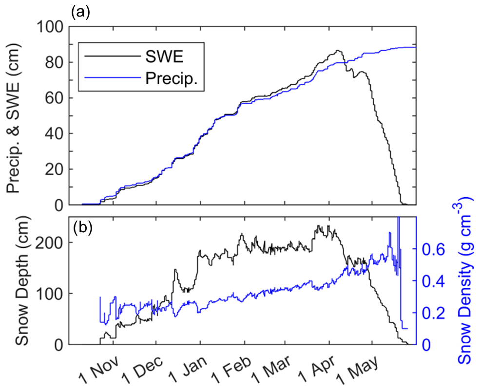
Figure 3 SNOTEL data for the 2023 water year showing (a) observed SWE and cumulative precipitation and (b) observed snow depth and calculated snow density.

2.6 SNOWPACK modeling

The SNOWPACK model (Bartelt and Lehning, 2002) simulates seasonal snowpack based on weather station data. This study uses SNOWPACK due to past studies validating the liquid water representation in the model structure (e.g., Wever et al., 2014). We used SNOWPACK to represent energy balance changes occurring on each aspect of the watershed to contextualize observations made in the field, with the primary objective of informing the researchers about the timing of snowmelt events. SNOWPACK discretizes the vertical snow profile into multiple layers to account for energy and mass transfer through the accumulation and melt phases of the snowpack. In addition to closing the mass and energy balances per time step, the model includes physically based routines for internal snowpack processes. Simulated snow depth, SWE, snowpack temperature, and stratigraphy have been extensively validated for SNOWPACK (Jennings et al., 2018b; Lundy et al., 2001; Meromy et al., 2015; Rutter et al., 2009). SNOWPACK has also been shown as a successful tool in predicting snow liquid water content (LWC) in previous studies (Wever et al., 2014; Würzer et al., 2017; Webb et al., 2021a).

Simulations were run at hourly time steps with quality-controlled observations of air temperature, relative humidity, wind speed, incoming shortwave radiation, incoming longwave radiation, and precipitation to simulate the accumulation and melt of a snowpack. The first simulation represents the flat terrain of the study area using mostly SNOTEL data. The second simulation represents the north aspect hillslope. The third simulation represents the south aspect hillslope near the exposed ridge at the top extent of elevation for the study area, using mostly RAWS station data (which is positioned on the ridge of the south aspect). Incoming shortwave radiation for each simulation used the RAWS station data and a location-specific multiplication factor determined by the 1 March solar radiation model from the 1 m DEM (Fig. 1c). The precipitation phase threshold was increased from the default SNOWPACK to a value of 2.5 °C because the Rocky Mountains of the western United States have some of the highest rain–snow thresholds in the Northern Hemisphere (Jennings et al., 2018a). Turbulent energy exchange was simulated using the bulk Richardson number approach as this stability correction produced the best model performance at another subalpine site in Colorado (Jennings et al., 2018b). We did not define soil layers in SNOWPACK simulations because the primary focus of the modeling component is to inform us of the timing of snowmelt events. Additionally, canopy was not considered in our modeling to represent general conditions for each terrain condition. Further details on parameter decisions for the SNOWPACK simulations are offered in Appendix C.

3 Results

3.1 Transect data

For the 2023 water year the SNOTEL peak SWE occurred on 6 April at 866 mm, followed by rapid decreases in snow depth and SWE. We found the flat terrain transect observations followed similar snow depth and SWE patterns to SNOTEL data. In this location, transect data showed similar peak snow depth but slightly lower SWE and ρ_s values during the 1 April survey (Fig. 4a). In general, the flat terrain transect data compared well with SNOTEL data.

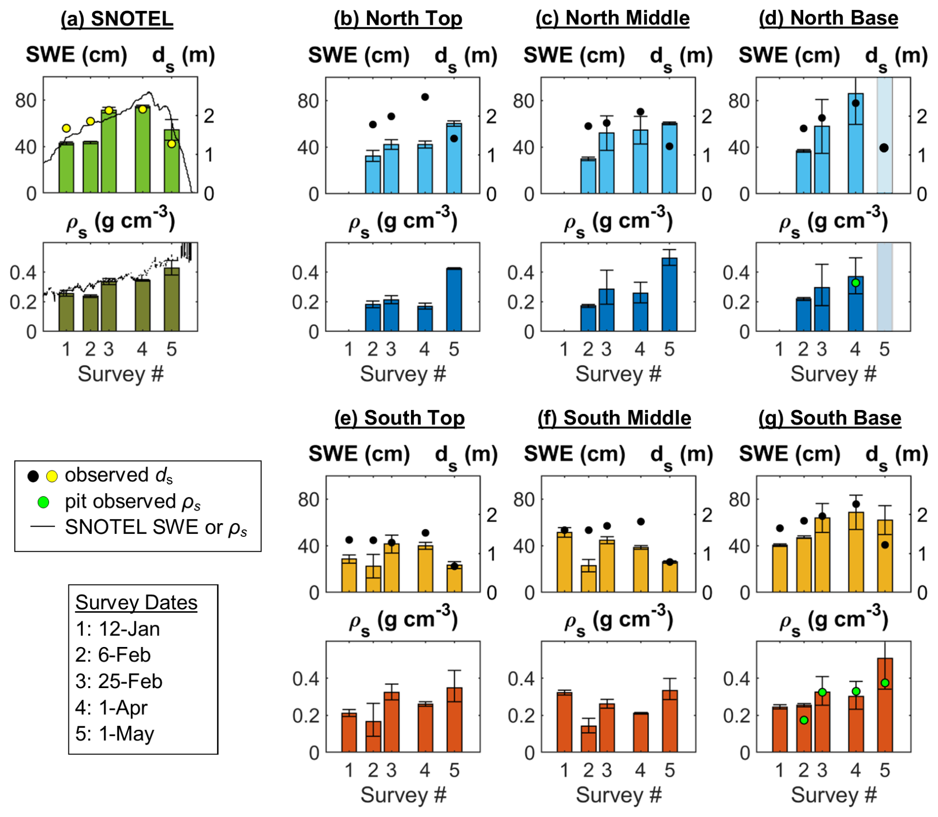
Figure 4 Results from the transect observations including calculated SWE, observed d_s, and GPR-derived ρ_s for (a) flat terrain around the SNOTEL station, (b) north top, (c) north middle, (d) north base, (e) south top, (f) south middle, and (g) south base locations. Pit measured average densities are shown when collected, and SNOTEL station data are displayed for additional comparisons of SWE and ρ_s. Uncertainty bars are shown for SWE and GPR-derived ρ_s using σ of collected data. Note that the GPR results that gave unrealistic values due to the presence of liquid water are slightly greyed in panel (d).

Snow depth on the north aspect follows a similar pattern to the flat terrain, with increases during the accumulation phase and a rapid decrease starting in April (Fig. 4b–d), though this period also resulted in large increases in ρ_s, indicating an increased rate of densification, while SWE increases slightly. North aspect d_s values are highest overall, with the top of slope consistently producing the deepest snow throughout the season (Fig. 4b). However, we observed two distinct patterns in ρ_s on the north aspect. The first pattern is for the top and middle of the north aspect slope, showing a relatively consistent ρ_s through the early surveys and a large increase of ρ_s for the May survey (Fig. 4b–c). The second pattern occurred at the base of slope, showing a consistent increase from February to April. This base of the north aspect also resulted in an unrealistic value during the May survey (Fig. 4d) that we interpret as being the result of excessive liquid water content due to a very low radar velocity and high relative dielectric permittivity (e.g., Bradford et al., 2009). This location has also been previously observed to result in excessive liquid water during spring snowmelt (Webb et al., 2018a), though no snow pit was dug at this location in May for the 2023 water year.

We found the south aspect transects had unique patterns relative to the flat terrain and north aspect during both the accumulation and melt phases of the snowpack (Fig. 4). The d_s values at the top and middle position of the south aspect show gradual increases from January to April, with both gains and losses in SWE during this time (Fig. 4e–f). The base of the south aspect sees a similar pattern of increasing depth, but with SWE consistently increasing from January through April surveys (Fig. 4g). All transects on the south aspect experienced a decline in SWE from the April to May surveys, though the smallest change occurs at the base of the south aspect, coinciding with a large increase in ρ_s at this location (Fig. 4e–g).

The variability in collected data showed average σ_TWT of 0.57 ns (4.5 %) and ${\mathit{\sigma }}_{d_{\mathrm{s}}}$ of 0.11 m (6.8 %). This resulted in an average uncertainty in mean ρ_s of 46.2 kg m⁻³ (17.0 %) and an average uncertainty in derived SWE of 6.1 cm (17.4 %) prior to calibration to snow pits and SNOTEL observations. These uncertainty averages do not include the base of the north aspect hillslope data from 1 May. Figure 4 shows this uncertainty associated with the ρ_s and SWE derived from GPR and manual d_s. The lowest variability was observed in the transect around the SNOTEL station (Fig. 4a), and the highest variability was observed at the base of the north aspect (Fig. 4d). The values of σ in collected data and resulting v, ε, ρ_s, and SWE for each transect are available in Appendix D.

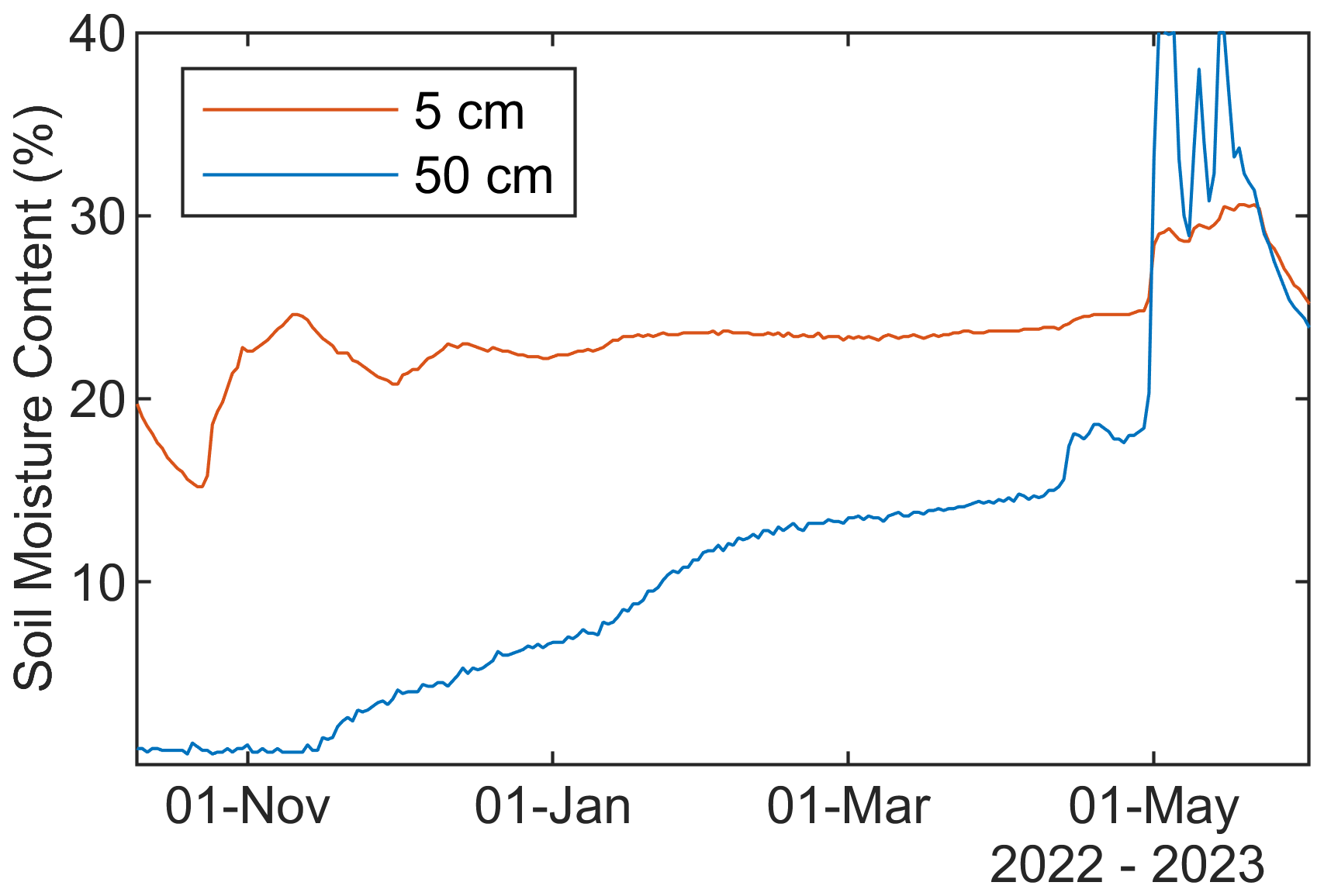
Qualitative observations were also noted during transect surveys, including surface melt on the south aspect forming small runnels in the afternoon during the 1 April survey. While wet snow was qualitatively observed in snow pits on other aspects as well, the south aspect was the only location that was observed to pond on layers and form snow surface runnels. We interpret this to indicate that the south aspect slope transports some liquid water laterally through the snowpack at times when other areas of the watershed do not. Additionally, soil moisture sensors at the SNOTEL station show a steady rise in soil moisture through snow accumulation, indicating a steady source of moisture throughout the winter (Fig. 5).

Figure 5 Soil moisture data from the SNOTEL site at depths of 5 and 50 cm.

3.2 Snow pit observations

In general, the snow pits show patterns of increasing density with depth and time, as expected, with ice lenses and layers forming from the upper to mid-snowpack in all pit locations (Fig. 7). The flat terrain pit did not have any ice lenses/layers in January, but one ice lens was observed in April that was approximately 3 cm thick and ∼ 230 cm above the ground (Fig. 7a). The north aspect only had a single snow pit observation during the 1 April survey, but 10 ice lenses/layers were observed throughout the snowpack from 30 to 210 cm above the ground – all were approximately 1–2 cm thick (Fig. 7b). Seven of the 10 observed ice lenses/layers were observed within a 70 cm section of the pit, from 110–180 cm above the ground (240 cm total pit depth). Pits dug at the base of the south aspect showed a single ice layer during the 28 February and 1 April surveys. This ice layer was approximately 4 cm thick at ∼ 150 cm above ground in February and approximately 11 cm thick ∼ 70 cm above ground in April (Fig. 7c).

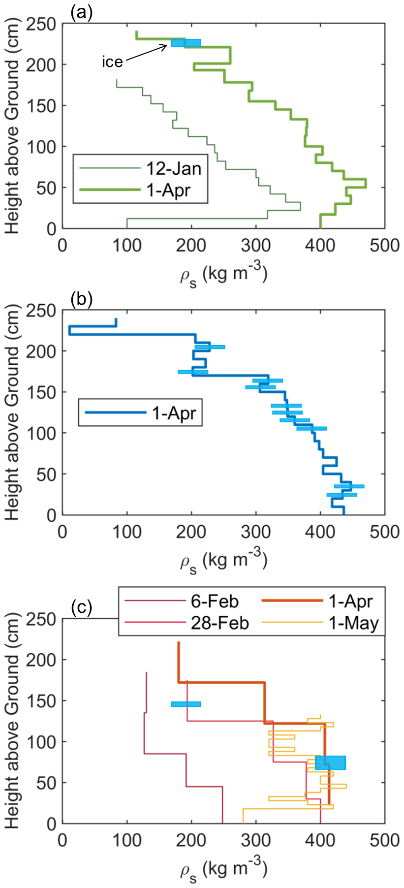
Figure 6 Snow pit observations of ρ_s and ice layers/lenses for (a) flat terrain, (b) north aspect, and (c) the base of the south aspect. We estimate an uncertainty of approximately 10 % for these density measurements.

3.3 SNOWPACK modeling results

Modeling of d_s, ρ_s, SWE, and snow LWC was completed using the SNOWPACK model to simulate accumulation and melt on the flat terrain, north aspect, and south aspect areas of the study site. The flat terrain simulation produced results matching the SNOTEL data well during accumulation, but with slightly different melt rates in May. The north aspect simulation resulted in the largest snow depths and longest snow persistence (Fig. 7a–b). The south aspect simulation showed the lowest snow depth and the earliest melt-out date. The simulated ρ_s in SNOWPACK is similar across each aspect until April when melt begins. SNOWPACK-simulated bulk ρ_s showed a root mean squared error of 48 kg m⁻³ when compared to pit-observed ρ_s. During the first two surveys (12 January and 6 February) SNOWPACK overestimated ρ_s, whereas it underestimated ρ_s during the late February and May surveys (28 February and 1 May). SNOWPACK-simulated ρ_s was within 10 kg m⁻³ of pit-observed ρ_s for all three pits on 1 April, representing a bias of less than 2 % near peak SWE. All model simulations indicate a spike in density prior to completely melting out, but with different amplitudes and timing. The simulated SWE shows similar patterns relative to SNOTEL data. SWE peaks in both the flat and south aspect simulations on 5 April (∼ 810 and ∼ 285 mm, respectively), the date of a snowstorm prior to a period of warmer weather, whereas peak SWE in the north aspect model occurred on 24 April at ∼ 920 mm. In comparing the SNOWPACK-simulated SWE to GPR-estimated SWE near simulated peak SWE dates, we see the flat terrain had an estimated 744 mm from GPR (833 mm from SNOTEL pillow) compared to a simulated 786 mm for 1 April (∼ 5 % difference), the north aspect slope had an estimated 603 mm compared to a simulated 813 mm (∼ 35 % difference), and the south aspect slope had an estimated 392 mm compared to the 265 mm simulated for 1 Apr (∼ 33 % difference). The SNOWPACK simulation captures the increase and decrease in SWE relative to the north and south aspect, respectively, with similar magnitude differences compared to transect estimates of SWE near peak SWE.

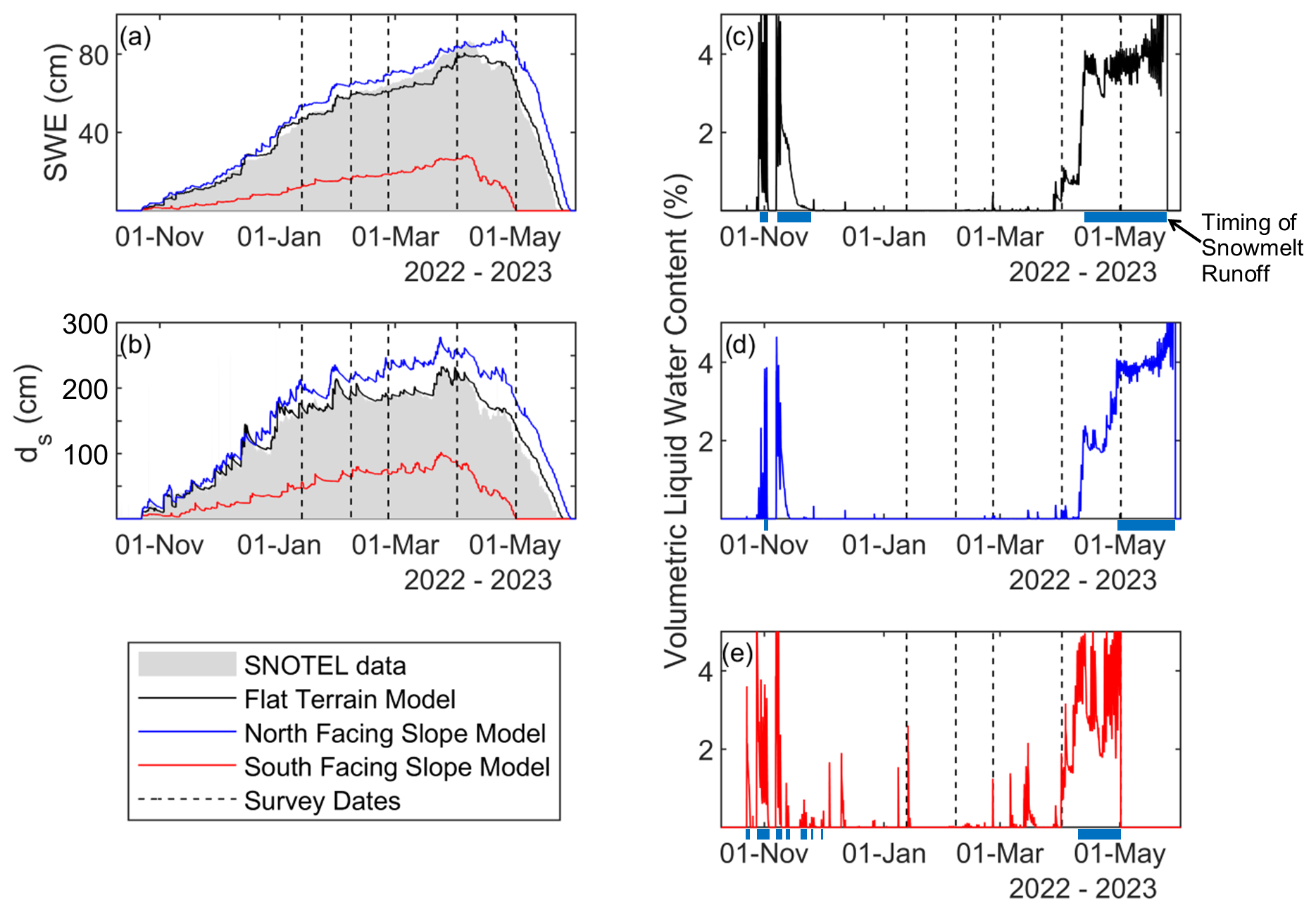
Figure 7 Results from the SNOWPACK simulations including (a) SWE, (b) d_s, and (c–e) volumetric liquid water content. Panels (c)–(e) also show when simulated snowmelt runoff from the snowpack is occurring as blue bars. Results show comparison to SNOTEL data as well as timing with survey dates.

All SNOWPACK simulations show intermittent surface melt events (Fig. 7c–d), with the largest and most regular occurring on the south aspect simulation (Fig. 7e). The flat terrain and north aspect simulations did not result in volumetric LWC values greater than 0.5 % for the period of December through March (Fig. 7c–d). However, south aspect simulated bulk volumetric LWC increases to 1 % or more nine times from December through March (Fig. 7e). Additionally, simulated LWC at the base of the snowpack, indicating timing of simulated snowmelt runoff, occurs only during the early accumulation season and after peak SWE for all simulations (Fig. 7c–e).

4 Discussion

This study observed snow density variation with aspect and position on slope using pit calibrated GPR transects. The results showed flat terrain transect data that matched well with SNOTEL d_s and SWE measurements (Fig. 4). The flat terrain SNOWPACK simulation results also matched well with observational data from the SNOTEL station as well as survey transect data (Fig. 7). SWE varied slightly from the measured to the simulated data, likely due to precipitation uncertainties relative to snow on the ground as observed by the snow pillow. The results of this study also suggest ponding of LWC in the snowpack at the base of the north aspect during the ripening and melt phase, whereas mid-season surface melt occurring on the south aspect hillslope is interpreted as redistributing SWE down towards the base of the slope. Variations in snow depth and density along both hillslopes have implications for SWE distribution and peak timing, indicating the importance of aspect-specific considerations for modeling of SWE and melt processes (Sexstone and Fassnacht, 2014; Lopez-Moreno et al., 2013).

4.1 Limitations of study

It is important to also discuss the limitations of the present study and potential ways to overcome these in future studies. The SNOWPACK simulations used could be further calibrated. In future studies the use of a multi-dimensional model could also be beneficial to further consider the influence of forest canopy and wind transport – factors that have been found to be just as important as aspect (Mazzotti et al., 2023). However, there is not currently a hydrologic model that incorporates lateral flow through snow, so more snow pits along with quantitative observations of LWC and lateral flow processes could further our understanding (e.g., Thompson et al., 2016). The use of sensors installed within a snowpack could also provide further time-series data (e.g., Díaz et al., 2017) to observe the presence and ponding of liquid water at locations of interest. These observations could provide more precise observations rather than the bulk estimates using the methods in the present study.

The uncertainty associated with the GPR and manual depth probing could also be improved using depth derived from lidar for more spatially continuous data. The magnitude of uncertainty found in the present study is similar to other studies pointing towards snow depth being the greatest source of uncertainty when using Eq. (3) (McGrath et al., 2022) and higher than other studies using lidar for snow depth (Meehan et al., 2024). The estimated uncertainty of ∼ 45 kg m⁻³ (prior to calibration) is similar in magnitude to the mean bias of 48 kg m⁻³ (mean absolute deviation of 60 kg m⁻³) of the transect ρ_s estimates relative to snow pit and SNOTEL data. This direct comparison was used for calibration due to the observation of liquid water being present in snow pit observations during surveys, indicating that the relative uncertainty of using Eqs. (1), (2), and (3) is likely lower than that estimated for dry-snow conditions along the transects of this study. After calibrating the transect ρ_s estimates to snow pit and SNOTEL data, the mean error was less than 5 kg m⁻³ (mean absolute deviation of 45 kg m⁻³).

4.2 Perceptual model

The Northern Hemisphere incidence angle of the sun allows for more exposure on the south aspect compared to the north aspect, which is shaded more of the time. This influences the energy balance of the snowpack by reducing energy inputs to the north aspect and increasing energy inputs to the south aspect, resulting in differences in accumulation and melt dynamics (Molotch and Meromy, 2014; Erickson et al., 2005). Additionally, the south aspect does not receive canopy shading in the winter because it is canopy-free in the top half of slope and is populated with deciduous aspen on the lower half of slope, which lose their canopy during the winter (Musselman et al., 2008; Varhola et al., 2010). There is some coniferous canopy on the north aspect slope, though the canopy is denser at the base of the slope. This difference in canopy cover is likely attributed to aspect as the deeper snow and increased soil moisture on the northern aspect increases the amount of plant available water for vegetation growth (Webb et al., 2023). However, transects were selected to have minimal canopy influence for hillslope observations, though this could not be accomplished at the base of the north aspect that did have some canopy shading.

The north aspect is an area of lower solar radiation exposure resulting in greater snow depths and later melt throughout the winter and spring seasons relative to other locations observed for this study. The north aspect hillslope is partially forested as well, which is likely a result of terrain shading and greater water availability during the growing season. This coniferous canopy remains intact throughout the winter months, providing shelter from wind and solar radiation, allowing snow to accumulate and persist longer. The survey transect higher up on the north aspect resulted in greater depths. Further down at the middle of the slope, depth decreases slightly with minimal SWE differences relative to the top of the slope. The transect in the middle of the north aspect has partial canopy coverage with parts near the drip edge of trees that likely resulted in some interception but also canopy sloughing that caused the lower depths and higher densities at this location relative to the top of the north aspect. The base of the north aspect is in a small opening of the mostly forested location of this study, though interception did not cause a large difference in accumulated snow depth (Fig. 4e). The most notable difference at the base of the north aspect is the steady increase in snow density through the observation period, with an unrealistic increase in ρ_s during the May survey (ρ_s > 1000 kg m⁻³). Once the snowpack begins to ripen, ρ_s spikes to values that are not physically possible, indicated by the GPR signal slowing, likely from liquid water in the snowpack. This could be a result of the exposed areas of the slope producing meltwater which flows downhill and ponds at the base of the slope as previously observed at this site (Webb et al., 2018a). Unlike the south aspect, here on the north aspect most of the SWE has remained on the hillslope through the winter, rather than melting intermittently with mid-season melt events. This excess of water on the north aspect slope, paired with shallow fine-grained soils with low infiltration capability, could explain ponding of liquid water at the base occurring with the onset of the melt phase. Snow pits dug on 1 April at the base of the slope further support this interpretation, as several ice lenses/layers distributed throughout the snowpack were observed, indicating the presence of multiple hydraulic barriers with the potential to divert liquid water laterally in the snowpack the entire length of the hill slope (Eiriksson et al., 2013; Webb et al., 2018b).

The increased exposure on the south aspect resulted in SWE losses from three mechanisms: melt, sublimation, and wind scouring. Wind sensors on the RAWS station indicate that wind speeds top out at 6–10 m s⁻¹, with most gusts coming from the northeast. The precipitation at this ridgeline sensor is lower compared to the SNOTEL sensors in the flats, likely a result of stronger winds blowing snow over the gauge. These kinds of wind could contribute to scouring of snow. Blowing snow is also more susceptible to sublimation (Vionnet et al., 2013). Modeling of snow depth and SWE on the south aspect are largely a product of precipitation input from RAWS data, resulting in lower values compared to measurements (Fig. 7). Melt-out dates reflect these lower precipitation inputs as well, with observable snow depth surveyed on 1 May, while the model simulated this as the last day of snow cover for the south aspect (Fig. 7). Despite model differences in melt-out dates, the simulated LWC parameter shows when surface melt occurred due to its root in physical processes and qualitative comparison to snow pit observations. The south aspect simulation reveals several mid-season surface melt events that were also qualitatively observed during surveys and were not present in the flat or north aspect models, which is a response to increased solar radiation exposure on the south aspect hillslope. These mid-winter surface melt events did not result in simulated LWC reaching the bottom of the snowpack. These mid-winter melt events on the south aspect also coincide with increased density at the base of slope (Fig. 4) and the formation and thickening of an observed ice layer (Fig. 6), which we are interpreting as an indication of likely downhill migration of SWE through intra-snowpack flow paths (Webb et al., 2020a; Webb et al., 2022; Eiriksson et al., 2013). The ice layer observed at the base of the south aspect is indicative of lateral flow in sloping terrain (Webb et al., 2018b; Schlumpf et al., 2024) as it is likely thick enough at 7 cm to create a hydraulic barrier and promote lateral flow. Observations of surface melt occurring on the south aspect also included small runnels forming late in the afternoon during the April survey, which further supports this interpretation. Additionally, soil moisture sensors at the SNOTEL station indicate a steady rise in soil moisture that aligns with snowpack accumulation, indicating a steady source of moisture throughout the winter (Fig. 5). With lateral groundwater fluxes from outside this watershed assumed to be negligible, the source of soil moisture rise is likely from melting snow on the south aspect as snow elsewhere in the watershed remains cold enough to not provide moisture inputs (Supplement Tables S1–S7). These results indicate the input of snowmelt from the south aspect may be providing connectivity to the stream and water sources to potentially maintain baseflow through the winter, though streamflow data are not available for this location. Further quantification of subsurface properties such as porosity and saturation of soils on the slope could clarify these processes and fully describe vadose zone hydrologic connectivity and water movement.

The energy balance proved to have a large effect on field data and modeling as the south aspect simulations encompassed greater energy inputs and exposure than the north aspect, resulting in different accumulation and melt dynamics. While these specific basin dynamics are not applicable to every snowpack, there are some general patterns that can be applied to areas with similar characteristics. For instance, (1) north aspects in this type of environment may experience lateral flow of water through snow and in the shallow subsurface, causing accumulation and ponding of liquid water at the base of the slope during spring ripening and snowmelt (Fig. 8b; Webb et al., 2018a), and (2) open-canopy south aspects that develop a seasonally persistent snowpack have greater potential for mid-winter melt events, interpreted in this study to cause a redistribution of SWE through liquid water transport downslope, increasing SWE and soil moisture (Fig. 8a). Figure 8 offers an update to the Webb et al. (2018a) perceptual model of these aspect controls on liquid water movement, with descriptions of the dominant processes during the winter and spring periods. Canopy and wind drifting influences are not interpreted as major contributions to the redistribution of SWE at Dry Lake due to the wind direction being parallel to the study slope contours and observations of drifting not occurring at our transect locations. However, some canopy shading will influence the observations at the base of the north aspect hillslope, though terrain shading dominates the energy balance as previously mentioned. Further, the deciduous canopy at the base of the south aspect has been observed to have more SWE than on the hillslope (Webb, 2017), but under-canopy conditions here generally have lower snow density, whereas we observed an increase in density at the base of the south aspect slope. Thus, we interpret the lateral flow of liquid water to be an important factor in the redistribution of SWE as presented in the perceptual model for the Dry Lake site (Fig. 8), though we are unable to fully disentangle the influence of canopy and lateral flow from one another.

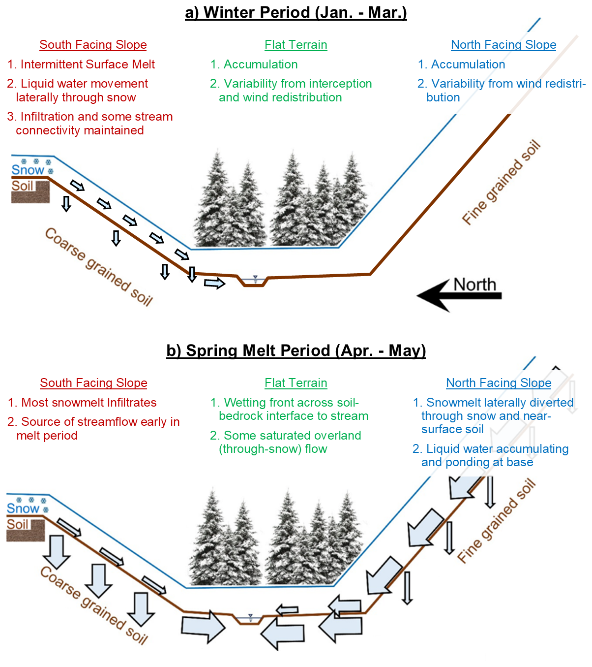
Figure 8 Perceptual model of interpretation of processes during (a) the winter period (January through March) and (b) the spring melt period (April through May). Panel (b) is modified from Webb et al. (2018a).

The main objective of this study was to determine how SWE and snow density change with aspect and position on hillslope. We found that sloped areas can have quite different melt dynamics which can greatly influence snow density. In particular, the base of slope seemed to be an area of greater SWE following different melt mechanisms (Fig. 8). Each aspect melts at different times because of varying energy balance dynamics. The north aspect experiences primarily accumulation during winter and distribution of mass through melt processes during the spring ripening and snowmelt periods in April, whereas the south aspect is responding to mid-winter melt, which is distributing mass to the base of slope during this time.

Assessing patterns in snow density and the influence of the movement of liquid water throughout a watershed and snow season can provide important context to measuring and modeling snow (Webb et al., 2022). Snowmelt and catchment liquid water input into a system have historically been associated with snowmelt rates; however, snowmelt rates are dependent on complex energy balance interactions between the snowpack and its environment. The traditional four-phase snowpack model of a homogenous snowpack going through accumulation, warming, ripening, and melt (Dingman, 2015) may not be representative of all snowpacks everywhere in a single watershed at a given time, especially when considering hillslope processes. Position on slope, aspect, and snowpack phases were found to be factors for snow density and presence of liquid water. Areas with higher energy input may see a greater range of density and more dynamic snowpack conditions. Paired with well-known depth variation, these parameters could have a compounding effect on SWE, further emphasizing the importance of quantifying the spatial variability of density at the catchment scale. Importantly, other studies have found that canopy structure and weather can be just as important as the topography component focused on in this study (Mazzotti et al., 2023). These results support further quantification of catchment-scale density for measurement of SWE, especially on different aspects as they have a significant influence on snowpack energy balance. Similar studies are needed to further understand density variation in systems with different energy balance dynamics or future projections of energy balance scenarios.

5 Conclusions

This study found that aspect produces snowpack melt and SWE distribution dynamics that are different from a traditional flat area one-dimensional perceptual model. In general, there is a pattern of downhill SWE migration and densification at the base of either hillslope which is largely influenced by energy input timing. Of these, the north aspect behaved more like the flat areas during the accumulation phase, with a large change at the onset of April melt interpreted to cause liquid water ponding at the base of the hillslope. The south aspect was found to be susceptible to mid-season melt events that increased snow density, which we interpret is occurring through the redistribution of SWE via the lateral flow of liquid water to the base of the hillslope. These differences between aspects are most related to solar radiation inputs.

Appendix A

In this Appendix, we present the wind rose produced for the observed winter and snowmelt season at the RAWS station (Fig. A1).

Figure A1 Wind rose for the Dry Lake RAWS site.

Appendix B

In this Appendix, we present the density methods that were used for each of the surveys (Table B1).

Table B1 Date and density measurement methods for each of the snow surveys.

Appendix C

In this Appendix, we provide further details of the SNOWPACK simulation parameterizations. We provide details in the tables below that describe common data sources and modeling decisions for all simulations (Table C1) as well as data sources and model decisions for the south aspect simulation (Table C2), flat aspect simulation (Table C3), and north aspect simulation (Table C4). If a parameter is not listed in the tables, then the default choice in SNOWPACK was used.

Table C1 Data sources and model decisions that are common to all SNOWPACK model simulations in this study.

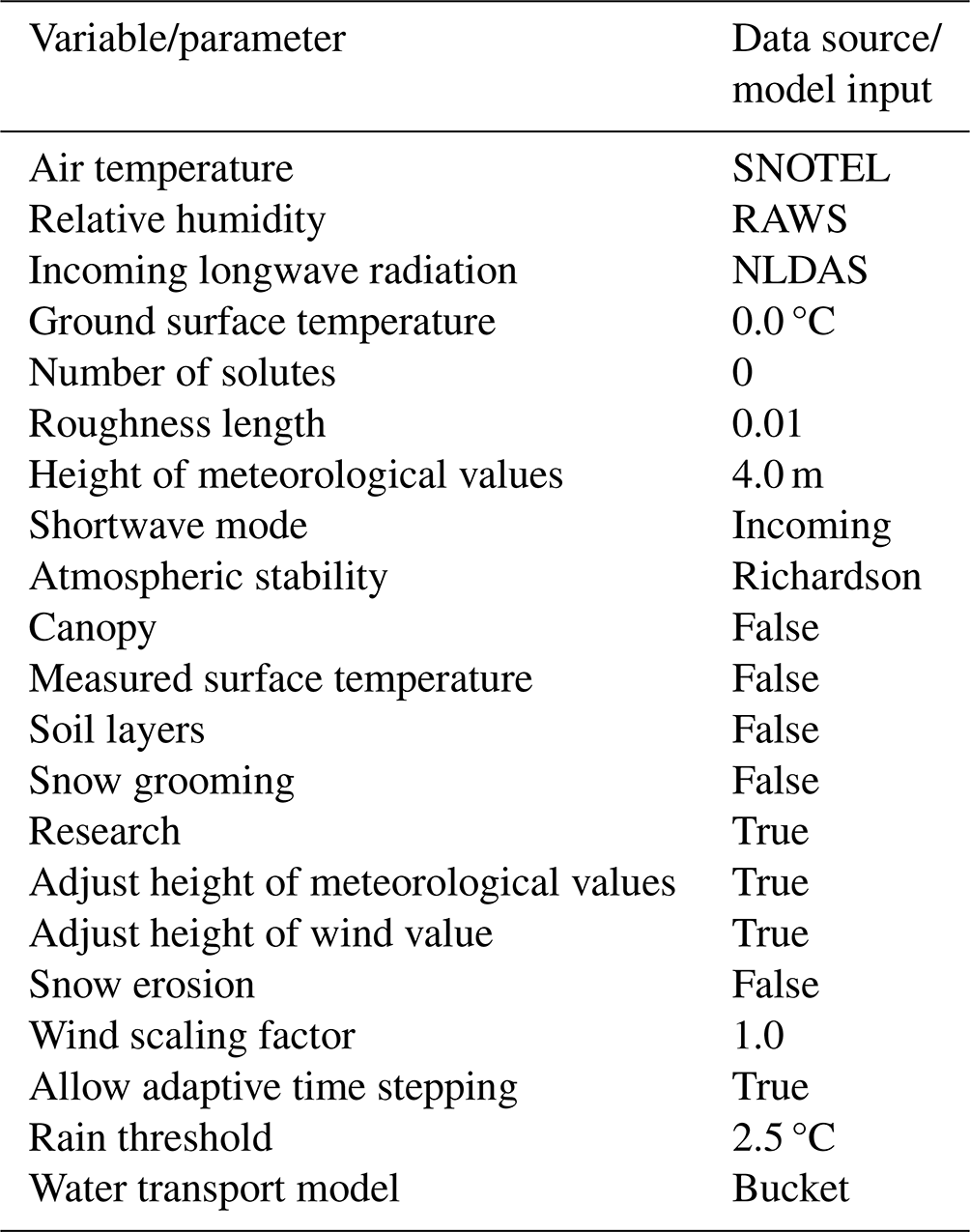
Table C2 Data sources and model decisions that were used for the flat aspect SNOWPACK model simulations in this study. Note that the shortwave radiation parameter includes the data source and multiplication factor discussed in the main text.

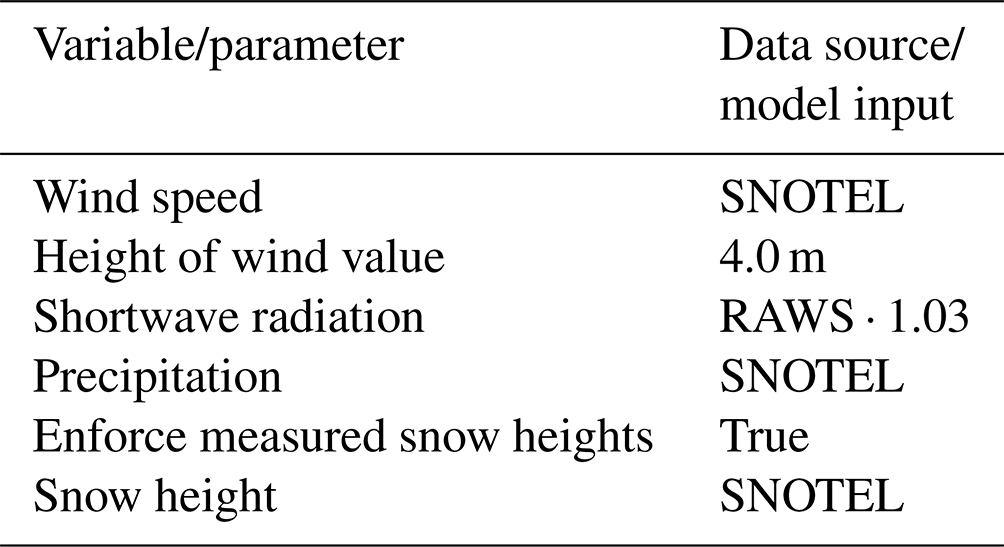
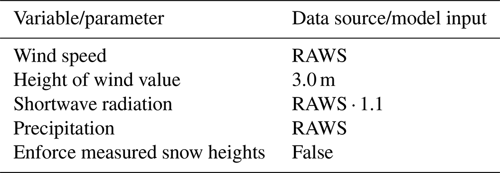
Table C3 Data sources and model decisions that were used for the north aspect SNOWPACK model simulations in this study. Note that the shortwave radiation parameter includes the data source and multiplication factor discussed in the main text.

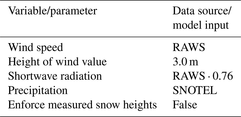
Table C4 Data sources and model decisions that were used for the south aspect SNOWPACK model simulations in this study. Note that the shortwave radiation parameter includes the data source and multiplication factor discussed in the main text.

Appendix D

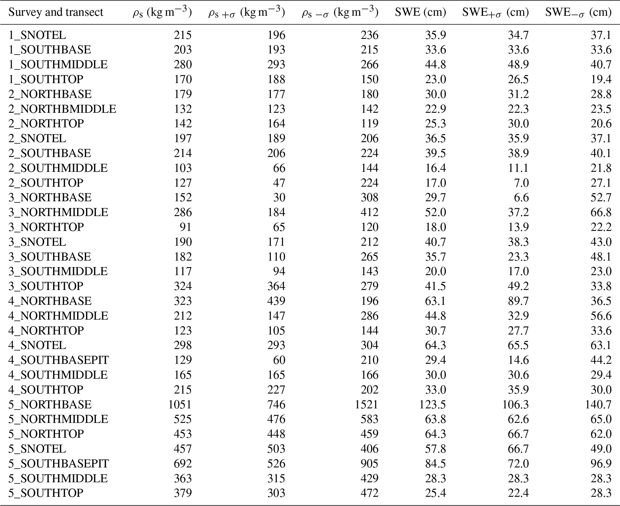
In this Appendix, we provide median GPR TWT and mean manually collected d_s for each transect as well as the σ for each survey. We then provide the results of using the data ±σ in Eqs. (1), (2), and (3) for the derived ρ_s and SWE estimates.

Table D1 Data collected including median GPR TWT, mean d_s, and the associated σ for each survey date and transect. Survey dates are indicated in order as numbers as follows: 1 for 12 January, 2 for 6 February, 3 for 25 February, 4 for 1 April, and 5 for 1 May.

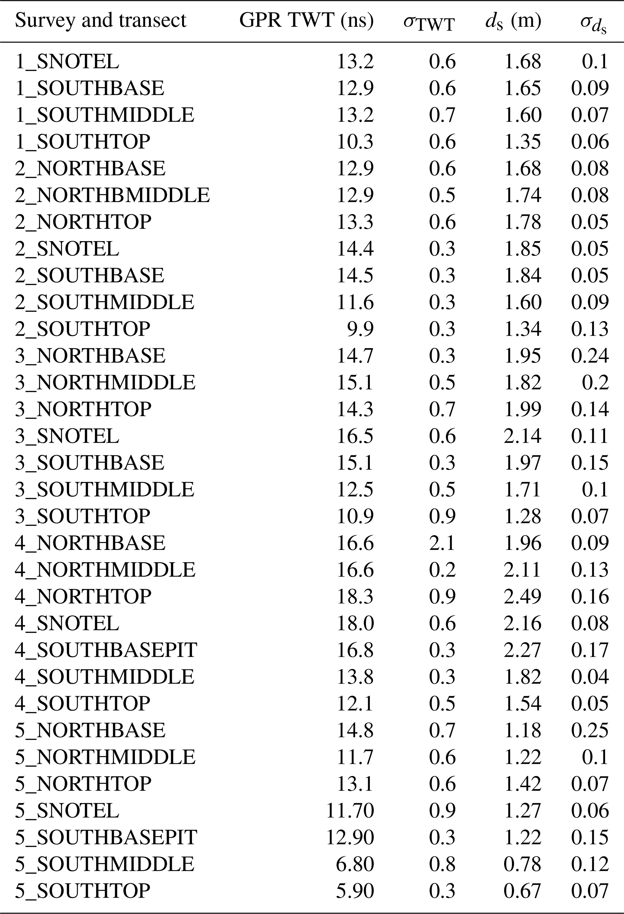
Table D2 Calculated v and ε values calculated using the mean/median data in addition to using the mean/median data ±σ. Survey dates are indicated as numbers as follows: 1 for 12 January, 2 for 6 February, 3 for 25 February, 4 for 1 April, and 5 for 1 May.

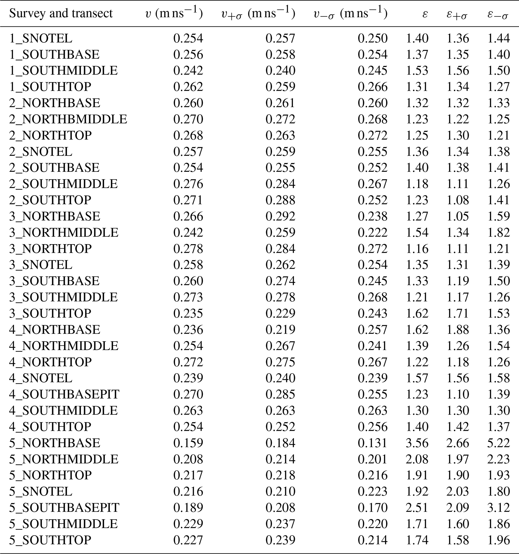
Table D3 Calculated ρ_s and SWE values using the mean/median data in addition to using the mean/median data ±σ. Survey dates are indicated in order as numbers as follows: 1 for 12 January, 2 for 6 February, 3 for 25 February, 4 for 1 April, and 5 for 1 May.