Trends in the annual snow melt-out day over the French Alps and Pyrenees from 38 years of high-resolution satellite data (1986–2023)

Information on the spatial–temporal variability of seasonal snow cover duration over long time periods is critical for studying the responses of mountain ecosystems to climate change. However, this information is often lacking due to the sparse distribution of in situ observations or the lack of adequate remote sensing products. Here, we combined snow cover data from 10 different optical platforms, i.e. SPOT (Satellites Pour l'Observation de la Terre) 1–5, Landsat 5–8, and Sentinel-2A and Sentinel-2B, to build a time series of the annual snow melt-out day (SMOD, i.e. the first day of no snow cover) at 20 m resolution across the French Alps and Pyrenees (43 × 10³ km²). We evaluated the pixel-wise accuracy of the computed SMOD using in situ snow measurements at 276 stations. We found that the residuals are unbiased (median error of 1 d) despite a dispersion (RMSE of 28 d), which suggests that this dataset can be used to study SMOD trends after spatial aggregation. We found average reductions of 21.4 d (5.78 d per decade) over the French Alps and 16 d (4.33 d per decade) over the Pyrenees over the period 1986–2023. The SMOD reduction is robust and significant in most parts of the French Alps and can reach 1 month above 3000 m. The trends are less consistent and more spatially variable in the Pyrenees. This dataset is available for future studies of mountain ecosystem changes and is updated every year using Sentinel-2 data.

1 Introduction

In mountainous regions, hydrological and ecological processes are strongly influenced by seasonal snow cover. As a result, ongoing snow cover changes due to global warming threaten the sustainability of numerous ecosystem services (Hock et al., 2019; Adler et al., 2022). Specifically, the annual snow melt-out day (SMOD, also named the snow cover melting day, i.e. the first day of no snow cover or the first no-snow day) modulates the onset of the vegetation growing season and therefore has a profound impact on soil processes, vegetation phenology, and productivity (Alonso-González et al., 2024; Choler, 2015; Francon et al., 2023; Jonas et al., 2008; Revuelto et al., 2022; Edwards et al., 2007; Choler et al., 2024).

The Copernicus Climate Change Service report on the European state of the climate highlights the fact that Europe is the fastest-warming continent in the world, with warming occurring at a rate twice that of the rest of the world (Copernicus Climate Change Service (C3S), 2024). In the French Alps from 1959 to 2010, the near-surface air temperature increased at a rate of 0.25–0.4 ± 0.2 ° per decade (Beaumet et al., 2021), consistent with rates reported in the rest of the European Alps (Hock et al., 2019; Rottler et al., 2019; Scherrer, 2020; Monteiro and Morin, 2023). In the Pyrenees, the near-surface air temperature increased by 0.2 °C per decade between 1959 and 2010 (OPCC-CTP, 2018). Previous studies have also identified long-term changes in the seasonal snow in European mountain areas (Notarnicola, 2022), including the Pyrenees (López-Moreno et al., 2020; Pons et al., 2010; Vidaller et al., 2021) and the Alps (Durand et al., 2009; Marty et al., 2017; Matiu et al., 2021; Scherrer et al., 2004; Schöner et al., 2019; Valt and Cianfarra, 2010; Dedieu et al., 2014). In the Mont Blanc massif, the highest peak of the European Alps, SMODs decreased at all elevations between the 2 decades 1965–1975 and 2005–2015 (CREA, 2024). However, little is known about the SMOD trends at larger scales in the European mountains, limiting our ability to understand and anticipate the responses of mountain ecosystems to climate change. As detailed below, this knowledge gap is due to the lack of observations of the extent of the snow cover on the land surface, or snow cover area (SCA), with the right combination of spatial and temporal density and extent, especially at high elevations (Hock et al., 2019). This work aims to fill this gap in the French Alps and Pyrenees.

We first defined the scientific requirements for computing SMOD trends in mountainous regions: (i) a spatial resolution lower than 100 m, (ii) a temporal depth exceeding 30 years, and (iii) an effective revisit frequency of better than 1 month. The first requirement comes from the complex topography of mountainous regions. In particular, the snow cover sensitivity to climate warming varies with the terrain slope and aspect (López-Moreno et al., 2014), and the spatial variability of mountain snow depth is typically within a range of less than 100 m (Blöschl, 1999; Mendoza et al., 2020; Trujillo et al., 2007). Hence, resolutions lower than 100 m are needed to decipher the influence of snow on alpine vegetation (Dedieu et al., 2016). The second requirement aims to limit the impact of natural climate variability such as the North Atlantic Oscillation, which extends to decadal scales in western Europe (Hurrell, 1995). In the European Alps and Pyrenees, the signs and magnitudes of snow cover trends become unstable if periods of less than 30 years are considered (López-Moreno et al., 2020; Monteiro and Morin, 2023). In general, a period of at least 30 years is recommended to enable the analysis of climate-driven snow trends (Bormann et al., 2018). The third requirement is motivated by the need to identify a SMOD with sufficient accuracy to analyse its trend, whose magnitude could be of the order of 1 week to 1 month over the past 3 decades (e.g. Hüsler et al., 2014; López-Moreno et al., 2020; Durand et al., 2008; Matiu et al., 2021). The accuracy of the SMOD is directly linked to the density of snow observations throughout the year (Hüsler et al., 2014).

We reviewed the different data sources that could be used to fulfil these requirements: in situ data, numerical snowpack modelling, and remote sensing. The in situ measurements have significant limitations due to the generally low number of long-term high-elevation sites and their uneven distribution (López-Moreno et al., 2020; Matiu et al., 2021). Stations above 2500 m are rare, representing 5 % of the stations used by Monteiro and Morin (2023) in the European Alps and 3 % of the stations used by López-Moreno et al. (2020) in the French Pyrenees. This hampers the interpolation of in situ trends at regional scales (Rohrer et al., 2013). Snowpack modelling can provide spatially continuous snow cover information. However, the temporal heterogeneity of the available meteorological data used for the atmospheric forcings can add biases to the long-term trends, especially in high-elevation regions, due to the scarcity of meteorological stations (Vernay et al., 2022).

Remote sensing is an effective tool for studying snow cover evolution over large regions. Advanced Very High Resolution Radiometer (AVHRR) data (1 km resolution) were used to determine snow cover trends since 1985 in the Alps (Hüsler et al., 2014). The MODIS instrument, active since 2000, allowed the production of a 500 m resolution dataset of daily global snow cover parameters (Dietz et al., 2015) and was used to show a negative snow cover duration trend of 17 d per decade across the Alps (Fugazza et al., 2021). The American Landsat program has provided an opportunity to map the snow-covered area at a higher resolution (60–30 m) since 1972, with each of the satellites from Landsat 1 to Landsat 9 capturing freely available images of continental surfaces with a revisit time of 16 d. The program kept two Landsat satellites active at the same time, improving the revisit time to 8 d (Loveland and Irons, 2016). This combination of available temporal depth and decametric spatial resolution unlocked new analyses of snow cover dynamics in mountainous regions (Choler et al., 2024; Bayle et al., 2023; Carlson et al., 2017; Margulis et al., 2016; Hu et al., 2020; Rumpf et al., 2022; Koehler et al., 2022a, b). Since 2017, our ability to characterize the snow cover evolution in mountains has progressed further with the Sentinel-2 mission, which offers a unique combination of systematic global coverage of land surfaces, a 5 d revisit time under consistent viewing conditions, high spatial resolutions (10, 20, and 60 m), and multi-spectral observations (Gascoin et al., 2019). Therefore, satellite remote sensing appears to be a promising and relevant method for addressing the objectives of this work. However, most satellite missions with freely available data fulfil only one or two of the requirements defined above. Despite their daily revisit times, MODIS and AVHRR spatial resolutions are not sufficient. The MODIS and Sentinel-2 periods of record are still too short. Landsat mission revisit times may be theoretically sufficient but are not guaranteed due to technical constraints (Ju and Roy, 2008; Zhang et al., 2022). Accounting for cloud cover, the effective revisit of Landsat is approximately one observation per month or less, which hinders applications in mountain ecosystems (Bayle et al., 2024b).

In 2015, the French Space Agency (Centre National d'Études Spatiales, CNES) started to open the archive of SPOT (Satellites Pour l'Observation de la Terre) images through the SPOT World Heritage (SWH) project. The SPOT program consists of five satellites, which observed Earth with three to four spectral bands with spatial resolutions of 10 and 20 m. SWH led to the release of nearly 20 million SPOT 1–5 products from 1986 to 2015. Since SPOT acquired images on demand, determining the average revisit frequency is challenging. Nevertheless, as acquisitions over western Europe were requested more often, we found that SWH significantly increases the number of available observations from Landsat only over the French Alps and Pyrenees (Barrou Dumont et al., 2023). In these regions, SWH offers the opportunity to enhance the temporal revisit of high-resolution multi-spectral imagery since the 1980s, thereby helping us to fulfil the above requirements. The low radiometric depth and the absence of a shortwave infrared band (SWIR) in SPOT images pose challenges for snow cover and cloud classification. However, we showed that this issue can be addressed efficiently using an image emulation approach to train a deep-learning algorithm (Barrou Dumont et al., 2024).

In this article, we merged the time series of SPOT, Landsat, and Sentinel-2 snow cover products to compute SMOD trends over the period 1986–2023, covering a domain of 43 × 10³ km² that includes the French Alps and Pyrenees at 20 m resolution (1.1 × 10⁸ pixels). We evaluated this new dataset using in situ SMOD observations in both mountain ranges. The combination of the high spatial resolution and the temporal depth of this dataset allowed us to analyse the spatial variability of the SMOD trend at fine spatial scales.

2 Data

2.1 Satellite products

We describe the satellite datasets following the remote sensing nomenclature which separates products by processing level. Level 1C refers to orthorectified top-of-atmosphere reflectances. Level 2B refers to a labelled image of the surface properties at the time of the acquisition, in this case three classes: snow, no snow, and cloud. The three collections of satellite data used in this work are SWH (SPOT 1–5), DLR-Landsat (Landsat 5–8), and the Theia L2 snow product (Sentinel-2A, Sentinel-2B, and Landsat 8) hereafter called Theia. We merged the SWH and DLR-Landsat datasets into a single dataset which we refer to as SWHLX.

2.1.1 SWHLX

SWH

Each SPOT satellite had two identical instruments. The first generation (SPOT 1–3) was equipped with twin High-Resolution Visible (HRV) instruments with green, red, and near-infrared (NIR) bands at 20 m spatial resolution. SPOT 4 was equipped with twin High-Resolution Visible and InfraRed (HRVIR) instruments which had the same geometric multi-spectral imaging characteristics as the HRV instrument but with the addition of a SWIR band of 20 m resolution. The SPOT 5 High Geometrical Resolution (HRG) twin instruments had the same multi-spectral characteristics as HRVIR except for an improved spatial resolution of 10 m for the three visible bands. The Theia data and services hub (https://www.theia-land.fr/product/SPOT-world-heritage-fr/, last access: 3 April 2024) provides a subset of 130 514 SPOT 1–5 60 km × 60 km images that were processed to Level 1C, mostly over French territory and Africa; 22 868 of these Level-1C images cover the French Alps and Pyrenees from 1986 to 2015 and were used in this study. We processed them to Level 2B using an algorithm which was designed to cope with the low radiometric quality of SPOT images and the lack of a shortwave infrared band in SPOT 1–3 (Barrou Dumont et al., 2024). This algorithm was marginally adjusted for this study to reduce an overestimation of the cloud mask. These adjustments are described in Appendix A.

DLR-Landsat

We used Level-2B products from Landsat 5–8 images of the Alps generated by Koehler et al. (2022a, b). They employed a modified threshold-based classification method (Hu et al., 2020, 2019b, a) to identify snow pixels using a decision tree that applies thresholds from the Normalized Difference Snow Index (NDSI) and Normalized Difference Vegetation Index (NDVI), along with a new index based on blue and NIR bands to better distinguish snow from clouds and other land features. Additional masking techniques for water bodies, topological shadows, and thermal thresholds were also implemented. We used these products for the period 1986–2015 (up to 2017 for Landsat 7). On average, these Landsat-derived Level-2B products achieved overall accuracies of 87.5 % for the Landsat 5 TM sensor, 95.5 % for the Landsat 7 ETM+ sensor, and 95.5 % for the Landsat 8 OLI sensor (Koehler et al., 2022a).

The DLR-Landsat dataset initially only covered the French Alps with 2916 products from five Landsat tiles (acquisition path/row combinations 195–196/28 and 194–196/29), each covering an area of approximately 173 km × 183 km. It was extended for this work with 3079 Landsat 5–9 images from five Landsat tiles (acquisition path/row combinations 198–200/30 and 197–198/31) covering the Pyrenees, reaching a total of 5995 Landsat 2B products. The Pyrenees images were selected and the 2B products generated following the same methodology as Koehler et al. (2022a, b). Landsat 4 images were not included in the study as their number was negligible in the area and period of study.

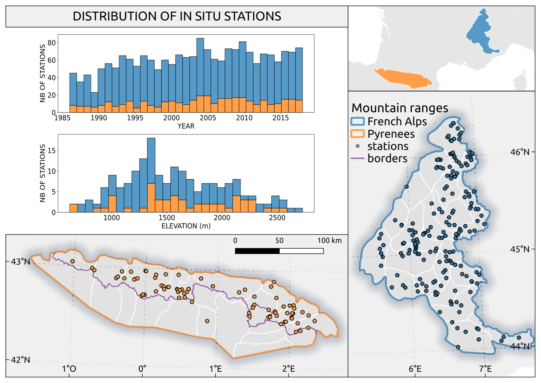
Figure 1 The 84 in situ snow depth stations' spatial distribution across the Pyrenees (left map) and the 192 stations across the French Alps (right map), together with their distribution across the years (top histogram) and elevations (bottom histogram). The bars of the histograms are stacked. The stations are from the Météo-France network, which is why only four stations are on the Spanish side.

2.1.2 Theia

For the period 2014–2023, we used the Level-2B products derived from Sentinel-2A, Sentinel-2B, and Landsat 8 that are routinely distributed by Theia (Gascoin et al., 2019). These products have been available over the study area since 2015 when the cloud fraction in the image is below 90 %. Landsat 8 processing was discontinued in August 2021. After that date, the only source of data is Sentinel-2. However, this only degrades the revisit time from 4 to 5 d. The SCA detection was evaluated in the French Alps and Pyrenees and had an accuracy of 94 % (Gascoin et al., 2019). A more comprehensive evaluation was conducted at a pan-European scale and yielded comparable results (Barrou Dumont et al., 2021).

2.2 Auxiliary data

The elevation of the analysed pixels was sourced from the Copernicus 30 m resolution digital elevation model GLO-30 (ESA and Airbus, 2022). The forest cover was derived from the Copernicus 20 m resolution tree cover density (TCD) for 2015 (EEA, 2018). The glacier areas were obtained from the Randolph Glacier Inventory (RGI) version 6.0, which provides the glacier outlines for 2010 (RGI Consortium, 2017). The water mask was derived from the Copernicus EU-Hydro river network database for 2006–2012 (EEA, 2020).

2.3 The in situ data

We used time series of snow depth at ground stations from the Météo-France network (Fig. 1). Each time series was obtained by assimilating in situ snow depth observations in a model run forced by the SAFRAN–SURFEX/ISBA–Crocus–MEPRA (S2M) reanalysis (Vernay et al., 2022). The assimilation method is direct insertion, which means that the reconstructed snow depth is equal to the observation when available. This method was developed to fill gaps in snow depth time series measurements due to sensor failures or the absence of a human observer (in the case of manual measurements). This dataset was previously used in the Pyrenees (López-Moreno et al., 2020). Station coordinates were not recorded with a consistent precision (between 10⁻¹ and 10⁻⁶°). Since the size of a 20 m pixel corresponds to the 10⁻⁴° order, only stations with a position precision of 10⁻⁴ and below were used. We excluded stations located in pixels with a tree cover density greater than 50 %, as done for the satellite data processing (Sect. 3.1). Some stations became active later in the study period, and other stations ceased activity earlier in the period, but, overall, the number of active stations increased over the years.

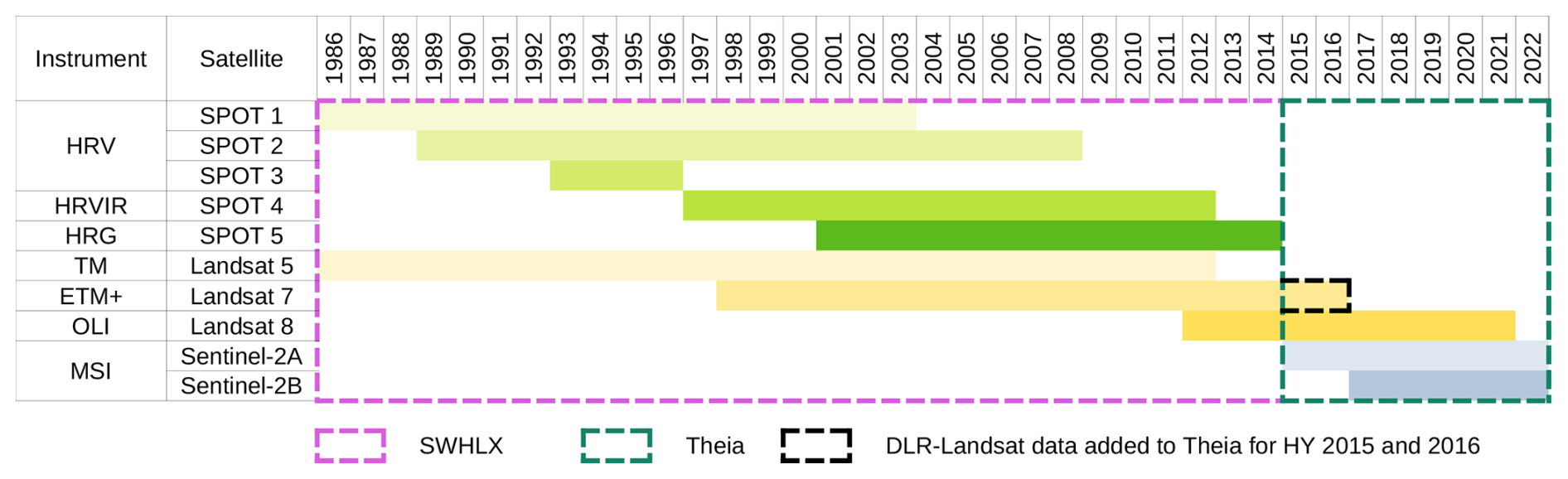
Figure 2 Satellite product distribution in the time series across the hydrological years. The dotted rectangles represent the dataset SWHLX (pink), Theia (green), and Landsat 7 products from DLR-Landsat (black) added to Theia.

3 Method

This section presents the method for generating 20 m resolution SMOD time series and their associated trends. SMODs were determined by hydrological year (HY), starting on 1 September. For example, the period between 1 September 2000 and 31 August 2001 referred to HY 2000, or 2000/2001. The trends were computed from combinations of SWHLX (HYs 1986–2014) and Theia (HYs 2015–2023) (Fig. 2). Since the SWH and DLR-Landsat datasets were generated from different approaches, we also evaluated their agreement using products that were generated from images acquired on the same day (see Appendix C1). The same thing was done between Sentinel-2 and Landsat 8 products for the Theia dataset (see Appendix C2). Then, we concatenated the SWHLX and Theia datasets. For HYs 2015 and 2016, the DLR-Landsat products (Landsat 7) were added to the Theia dataset to compensate for the absence of Sentinel-2B (launched in 2017).

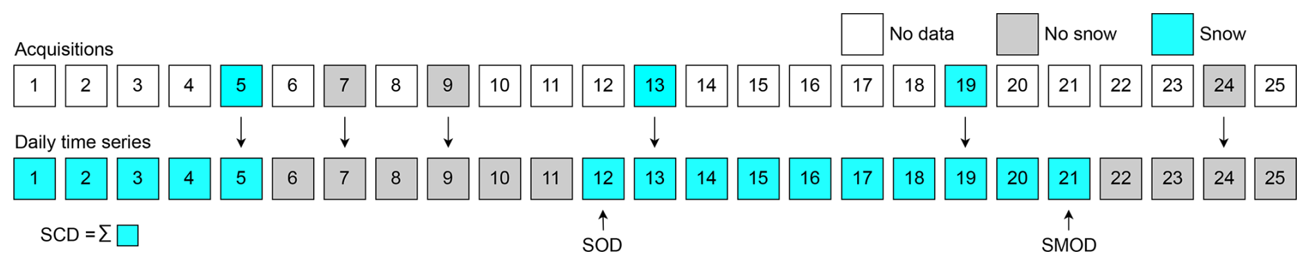
Figure 3 The 25 d hydrological period of snow, no-snow, and no-data days representing how snow periods are interpolated. The longest snow cover duration (SCD) starts with the snow onset day (SOD) on day 12 and ends with the snow melt-out day (SMOD) on day 21.

3.1 Calculation of the snow melt-out day

We defined a SMOD as the last day of the longest uninterrupted snow-covered period in the hydrological year (Monteiro and Morin, 2023). All SPOT and Landsat products were re-projected using a nearest-neighbour interpolation and cropped to the same reference system as Sentinel-2 products, i.e. a 20 m resolution grid of 110 km by 110 km in the Universal Transverse Mercator organized by tile and called the Military Grid Reference System. To obtain a daily time series of snow and no-snow labels from the Level-2B product time series, we used a nearest-neighbour interpolation between snow (1) and no-snow (0) observations in the time dimension (Fig. 3). For cases of odd numbers of days between a snow day and a no-snow day, the central day was considered a no-snow day. This process also filled missing data due to cloud cover or the failure of the scan line corrector in Landsat 7 imagery. For the Theia dataset, we interpolated daily values near the beginning and end of each HY by using Level-2B Theia products found within a margin of 15 d outside the HY. We observed that this method was insufficient with SWHLX in some areas with a short no-snow season due to its shorter revisit time. Hence, we assumed that persistent snow cover is negligible outside the glacier areas as defined by the RGI and assigned all non-glacier pixels the no-snow label on the day before and the day after each HY to improve the interpolation near the beginning and end of the HY in the case of a long period without observations. For cases where two Level-2B products from different sensors were available on the same day, the products were merged into a single raster by giving priority to (i) clear-sky observations and (ii) the pixel value from the highest-resolution sensor. For example, a SPOT snow pixel (20 m) had priority over a Landsat no-snow pixel (30 m), but a Landsat no-snow pixel had priority over a SPOT cloud pixel. Finally, we marked as no-data days the SMOD pixels whose tree cover density was greater than 50 % or which were located in the glacier mask or water mask.

3.2 Evaluation of snow melt-out days

We evaluated the satellite-derived SMOD from SWHLX and Theia with in situ SMODs (Sect. 2.3). To compute the in situ SMOD from the reconstructed in situ snow depth time series (Sect. 2.3), we used a snow depth threshold HS₀ to separate the daily snow depths into binary snow or no-snow labels. That is, a snow label was assigned if the snow depth was greater than or equal to HS₀. We used a HS₀ value of 1 cm as it was already identified as the best threshold for Sentinel-2 snow products (Barrou Dumont et al., 2021). We tested the sensitivity of the results to HS₀ with increments of 1 cm and found no significant differences for values below 5 cm (not shown here). Then, we computed the SMOD for each hydrological year from the same definition, i.e. the last day of the longest uninterrupted snow period. We excluded every SMOD value which coincided with a missing value in the original observed time series, since they were reconstructed using the model at that time step. In this way, we only evaluated the satellite SMOD with observed values, but we still took advantage of the entire reconstructed time series to identify the longest uninterrupted snow period. The agreement between the in situ and satellite SMODs was evaluated using the statistical distribution of the residuals for every hydrological year at each station's ΔSMOD (Eq. 1):

$$\begin{array}{}\text{(1)}& \mathrm{\Delta }\mathrm{SMOD}={\mathrm{SMOD}}_{\mathrm{year},\mathrm{station}}^{\mathrm{satellite}}-{\mathrm{SMOD}}_{\mathrm{year},\mathrm{station}}^{\mathrm{in}\mathrm{situ}}.\end{array}$$

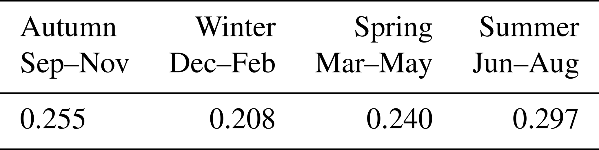
The SMOD accuracy is expected to increase with the number of clear-sky observations, as a higher number of clear-sky observations reduces the importance of the interpolation in the SMOD calculation. Therefore, we sought to establish a relationship between the number of annual clear-sky observations (NOBS) and the SMOD errors. However, our in situ dataset did not sample the full distribution of the topography in the study region. Thus, we generated an additional reference dataset from the Theia products, taking advantage of the high revisit of combined Sentinel-2 and Landsat 8 acquisitions to produce a spatially distributed reference SMOD dataset. We selected all Theia Level-2B products of tile 31TCH (Pyrenees) for HY 2017. We randomly sampled a subset of these products, following the seasonal probability of SPOT and Landsat acquisitions during the period 1986–2014. This probability was obtained by normalizing the seasonal distribution of SWHLX data from HY 1986 to HY 2015 (Table 1). From this undersampled time series of Theia products, we re-computed the SMOD and NOBS. The process was repeated by incrementally increasing the sampling size from 10 images to the number of available Sentinel-2 images minus 1. At each increment, the random sampling was repeated five times. This generated dataset allowed us to study the relationship between the sampled ΔSMOD and NOBS values. To characterize the SMOD errors, we used the median absolute error (MAE), the root mean square error (RMSE), and the interquartile range (IQR) (Appendix B).

Table 1 Seasonal weights used to sample Theia products to emulate SWHLX acquisitions over tile 31TCH.

We also evaluated the temporal stability of the SMOD error, because a time-dependent error could create spurious trends (Bayle et al., 2024b). Hence, we analysed the temporal evolution of ΔSMODs at two stations where SMOD values are available over the entire study period while respecting the minimum number of observations that we defined as a threshold for computing trends (see Sect. 3.3).

3.3 Snow melt-out day trends

SMOD trends were computed using a Mann–Kendall (MK) test of the combined time series of SWHLX and Theia. The MK test is a method for detecting consistently increasing or decreasing trends in temporal series (Kendall, 1948; Mann, 1945) and is often used in snow hydrology, including SMOD trend analysis (Klein et al., 2016; Nedelcev and Jenicek, 2021; Wang et al., 2016; López-Moreno et al., 2020). We used the Python implementation pymannkendall (Hussain and Mahmud, 2019) to compute the MK test and the slope of the trend using the Theil–Sen method (Sen, 1968). We considered a trend to be statistically significant if its p value was below 0.05. To evaluate the distribution of trends by elevation, we discretized the digital elevation model with the same 300 m elevation bands as those of the SAFRAN system (Durand et al., 1999). The analysis was stratified by a region of approximately 1000 km² and within each massif by topographical class (Fig. 4). The regions called “massifs” are relatively homogeneous with respect to their principal climatological characteristics at a given elevation, slope, and aspect (Durand et al., 1999). We restricted this analysis to elevation bands at 1500 m ± 150 m and above to focus on areas of seasonal snow cover. As a reference, in the Pyrenees, there is snow on the ground at least 50 % of the time between December and April at elevations above 1600 m (Gascoin et al., 2015). For every triplet of year, massif, and elevation band, we calculated the median of all the corresponding SMOD pixel values (no glaciers, TCD ≤ 50). We excluded the triplets for which less than 1000 valid SMOD values were available. For every combination of massif and elevation band, a trend was obtained by calculating the Sen slope from the SMOD time series.

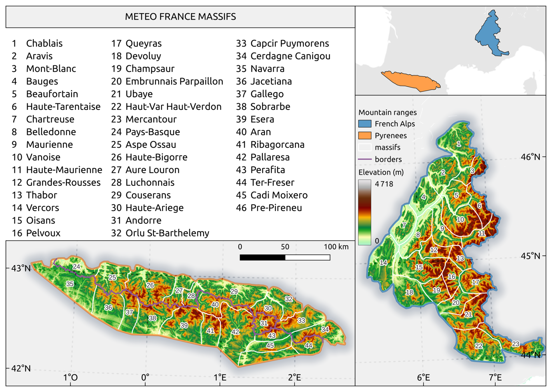
Figure 4 Pyrenees and French Alps divided into 23 massifs each. Massifs 35–46 are on the Spanish side of the Pyrenees (except for Andorra).

Trends were also calculated using the classes of topographical aspect and diurnal anisotropic heat (DAH). DAH represents the distribution of the heating of the surface by the Sun. It has been used to study snow spatial variability during the ablation season (Cristea et al., 2017) and plant growth responses to changes in snow cover at above-treeline elevations (Choler, 2023). It can be approximated by Eq. (2) (Böhner and Antonić, 2009), where a is the aspect of the slope, β is the slope angle, and α_max is the aspect with the maximum total heat surplus after a day–night cycle.

$$\begin{array}{}\text{(2)}& \text{DAH}=\cos ({\mathit{\alpha }}_{\text{max}}-a)\times \arctan \mathit{\beta }\end{array}$$

We used α_max = 212° (a direction between south and south-west) following Bayle et al. (2024a).

Since the accuracy of SMOD is expected to decrease when the number of observations is low, we only considered the cases when NOBS was above a threshold. This minimum NOBS threshold (NOBS_min) was applied in the SMOD pixel selection process before calculating the SMOD medians. However, a high NOBS_min threshold might prevent the calculation of SMOD medians for some combinations of massif and elevation band, especially in the years 1986 and 1987, when the available acquisitions were lower. Hence, we assessed the sensitivity of SMOD medians and their availability to NOBS_min.

Another source of uncertainty is the interannual variability, which can create spurious trends if the period of trend calculation is too short with respect to the natural variability. To test the robustness of our SMOD trends to the study period, we computed a trend matrix of every possible time period of 20 HYs or more between 1986 and 2022 for every combination of massif and elevation band. The trend of a period was only calculated if the SMOD median values of the first and last HYs of the period were available and if at least 95 % of the period's years were available (19 years for a period of 20 years, 35 years for a period of 37 years).

4 Results

The first part of this section presents an evaluation of SMODs obtained from both SWHLX and Theia against in situ data, together with a study of their uncertainties. The second part answers the second question of this work and leverages the high spatial resolution of the data to establish SMOD trends for HY 1986 to HY 2022 stratified with respect to the massifs delimited by Météo-France and the topographical classes.

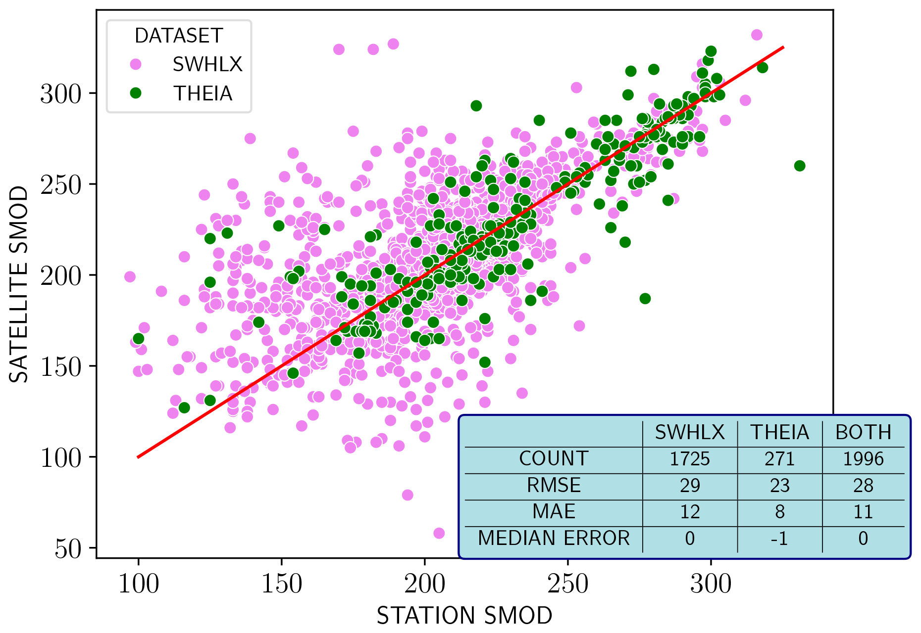
Figure 5 Scatterplots between satellite-based SMODs and station SMODs at HS₀ = 1 for the combination of Theia and SWHLX between HYs 1986 and 2018.

4.1 Evaluation of snow melt-out days

Our in situ data spanned HYs 1986 to 2018. With HS₀ = 1 and for the Theia dataset, we found an MAE of 8 d, an RMSE of 23 d, and a median ΔSMOD of −1 d (Fig. 5). Combining Theia and SWHLX gave an MAE of 11 d, an RMSE of 28 d, and a median ΔSMOD of 0 d. Both SWHLX and Theia performed better at higher SMODs, corresponding to June and July (i.e. above 275 d).

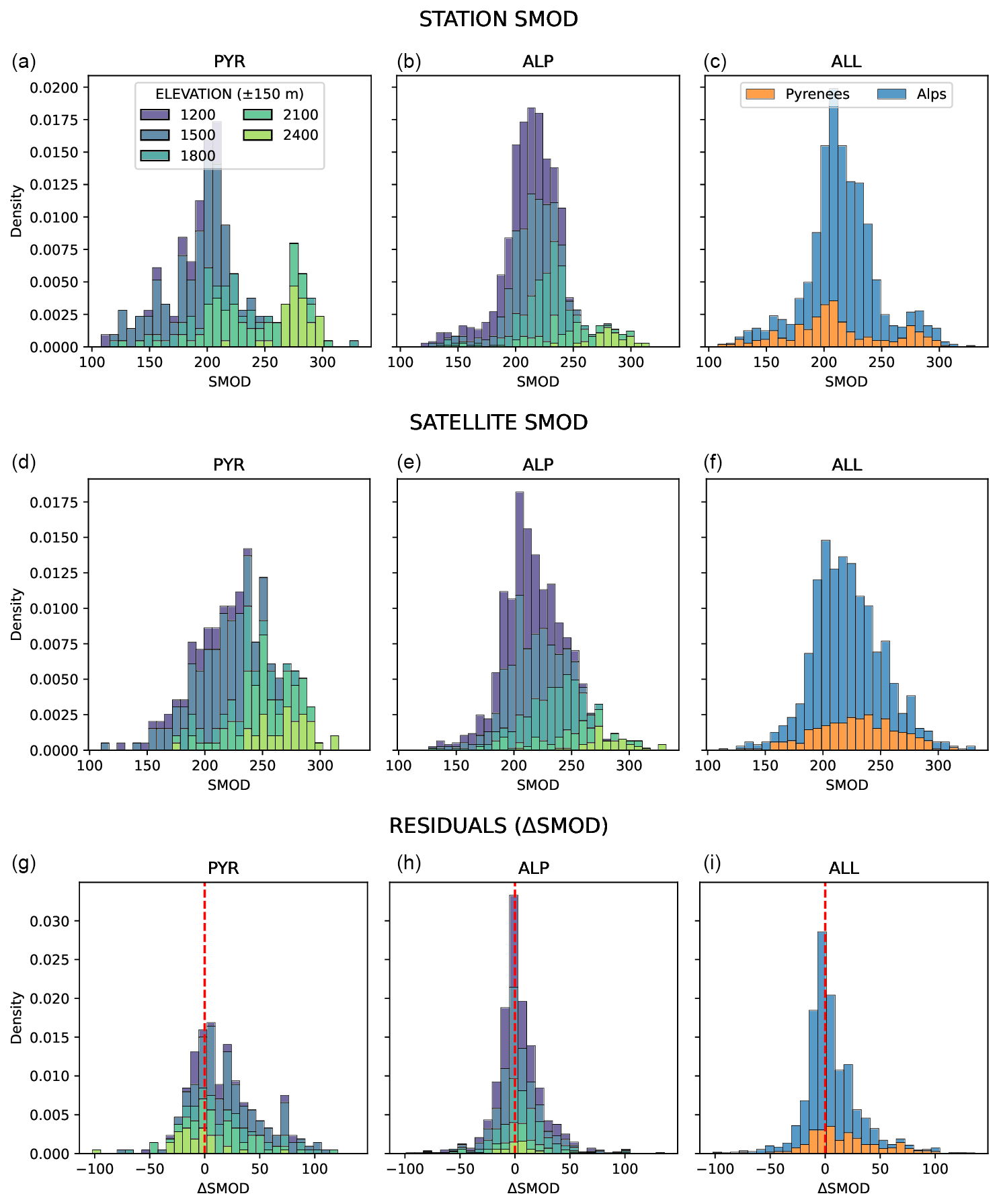
Figure 6 Normalized histogram of the in situ SMOD, satellite (SWHLX + Theia) SMOD, and residuals (ΔSMOD) stratified by elevation bands in the Pyrenees (a, d, g) and Alps (b, e, h). The right column (c, f, i) compares both mountain ranges.

Both in situ and satellite-based SMODs tended towards 200 (19–20 March) at lower elevations (1200 ± 150 m) and up to 280 (7–8 June) at 2400 ± 150 m (Fig. 6). We observed no significant bias towards an overestimation or underestimation with satellite-based SMODs in the Alps, but we observed an overestimation in the Pyrenees for every available elevation band except for 2400 m. This calls for caution when interpreting trends in the Pyrenees. The better performance in the Alps contributed to the overall results due to the lower number of in situ data in the Pyrenees and their lower elevation. From both stations which provide a SMOD reference value over the full study period, we did not find a clear trend in the evolution of the bias over time (Fig. D1).

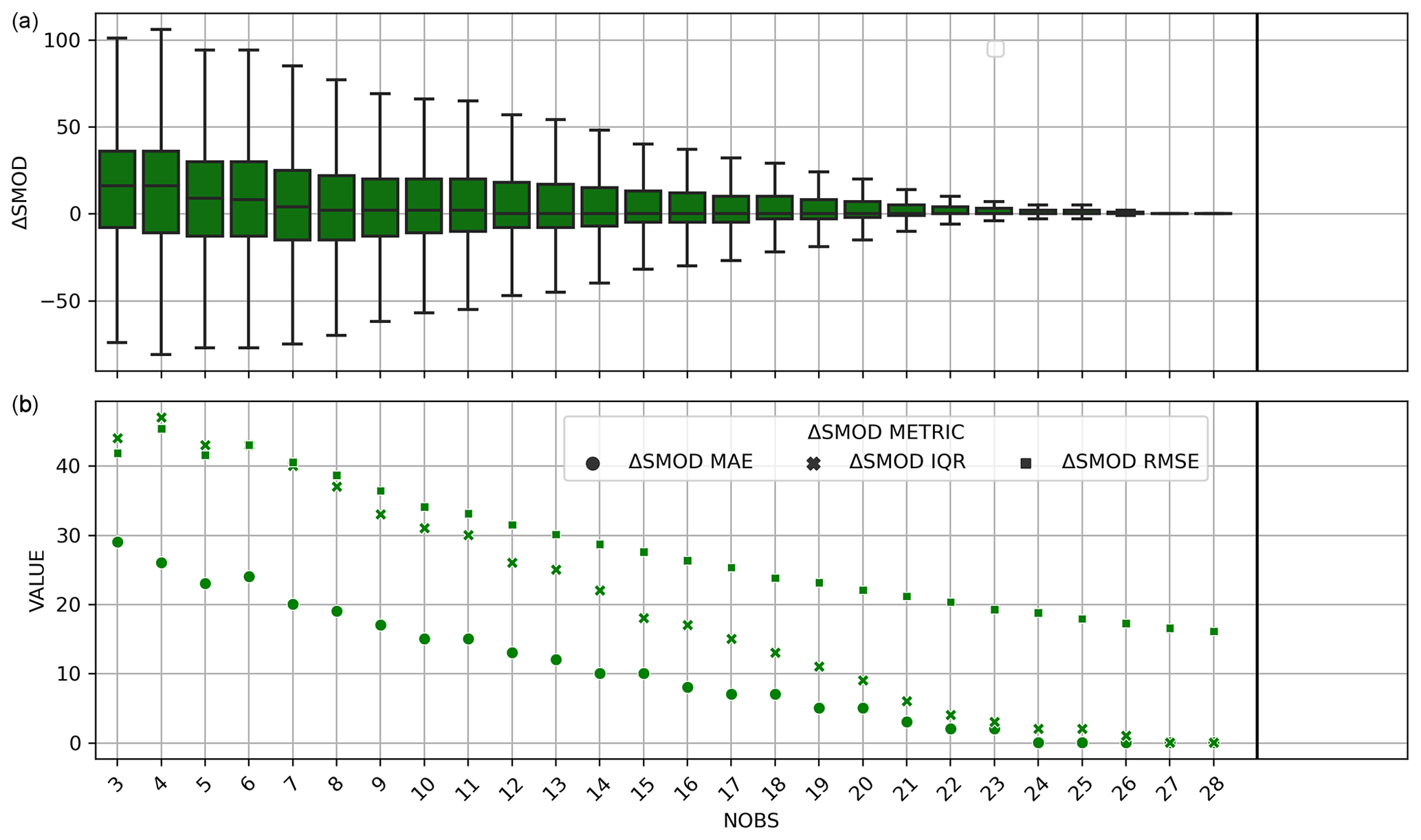
Figure 7 (a) ΔSMOD distribution per NOBS from the synthetic dataset derived from Sentinel-2 over the 31TCH tile for HY 2017. (b) ΔSMOD MAE, IQR, and RMSE per NOBS from the synthetic dataset derived from Sentinel-2 over the 31TCH tile for HY 2017.

The synthetic dataset derived from the Theia products allowed us to sample a larger number (> 10 000) of data (Fig. 7). We found an error variance that was significantly higher than 0 for NOBS ≤ 26 and a bias for NOBS ≤ 11 which starts increasing for NOBS ≤ 7. Excluding outliers, ΔSMOD was below 30 d for NOBS ≥ 19. We observed a negative correlation between NOBS and the different error metrics for NOBS ≤ 26 (Fig. 7). Beyond NOBS = 26, the error metrics were less sensitive to the NOBS value.

4.2 Snow melt-out day trends

Based on the previous analysis, we selected NOBS_min = 10 as the threshold before aggregating SMOD values by region and computing the SMOD trends. We found that higher NOBS values led to a significant reduction in the available combinations of HY, massif, and elevation bands from which a SMOD median could be calculated (Fig. D2 in the Appendix). Despite the large error that can be obtained with NOBS = 10 at the pixel level, the median values by massif and elevation band were similar to the ones that can be obtained with a higher NOBS_min (Fig. D3 in the Appendix). For these reasons, NOBS_min = 10 was chosen to report the results below, but we repeated the analysis with higher values and found similar results, albeit with more gaps.

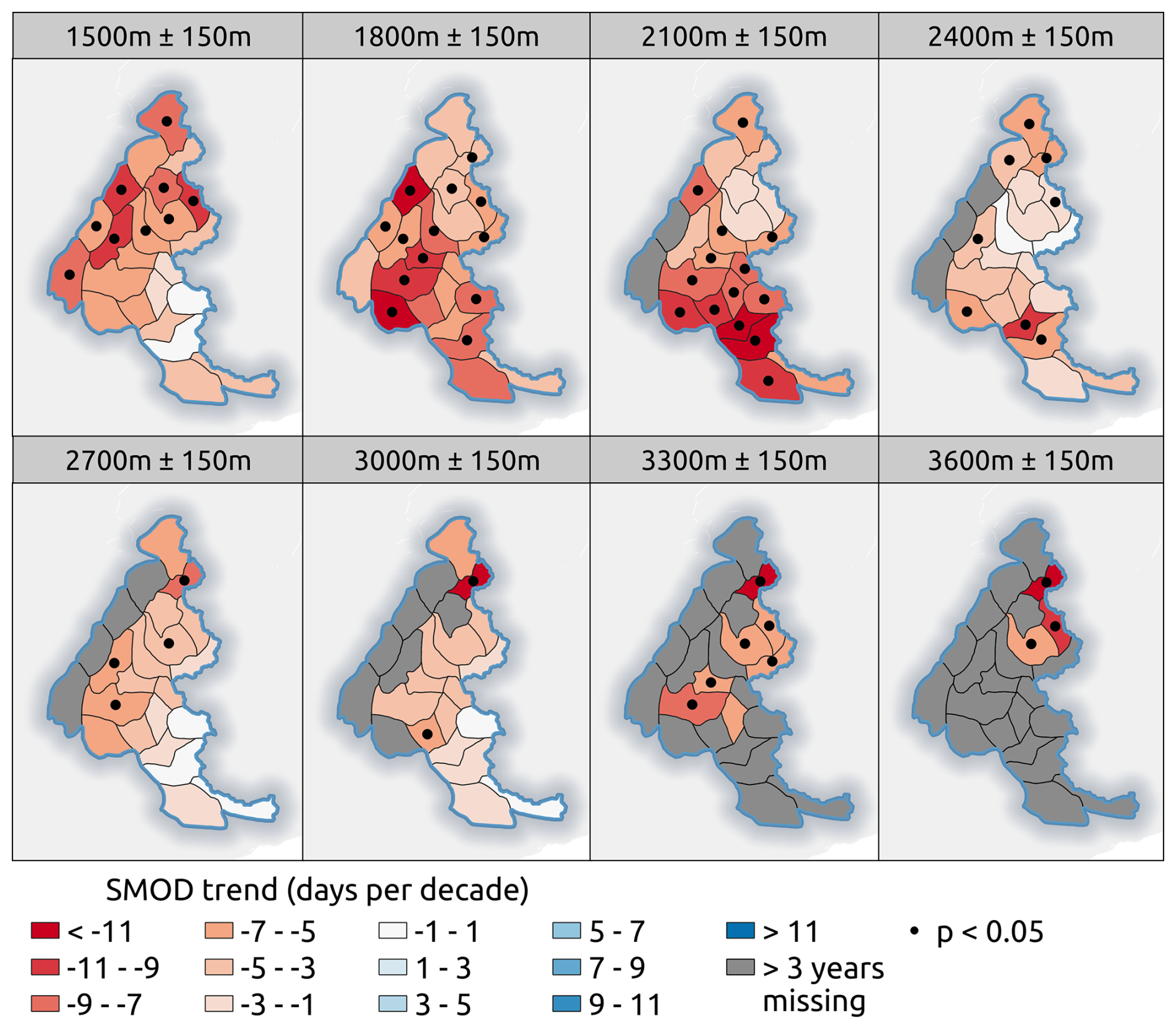
Figure 8 French Alps massif-wise SMOD trends for HYs 1986 to 2022. SMOD values were aggregated from ≥ 1000 pixels with NOBS_min ≥ 10. Areas are grey when less than 35 years of SMOD data were available due to us not having enough pixels or due to non-existent elevation bands. Dots identify statistically significant trends (p value < 0.05).

For HYs 1986 to 2022, all statistically significant trends were negative. In the French Alps, non-significant trends were either negative or less than ± 1 d per decade (Fig. 8). Significant negative trends were mostly seen in the northern massifs at 1500 m, in the central east at 1800 m, and in the central south at 2100 m. The trends generally became weaker at 2400 m and stronger again at 2700 m and above. At 2400 m and above, the Mont Blanc massif had a consistently significant decreasing trend which reached −14 d per decade at 3000 m.

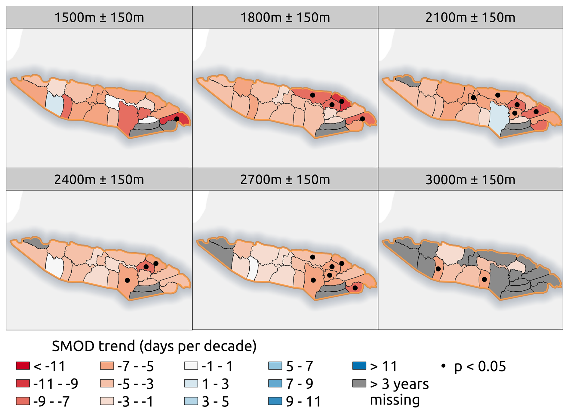
Figure 9 Pyrenees massif-wise SMOD trends for HYs 1986 to 2022. SMOD values were aggregated from ≥ 1000 pixels with NOBS_min ≥ 10. Areas are grey when less than 35 years of SMOD data were available due to us not having enough pixels or due to non-existent elevation bands. Dots identify statistically significant trends (p value < 0.05).

In the Pyrenees, all statistically significant trends were also negative and mostly found in the eastern half (Fig. 9). The Pre-Pireneu and Cadi Moixero massifs were not represented because they were not sufficiently covered by the Sentinel-2 tiles. Negative trends were less pronounced than in the Alps, and non-significant positive trends were also observed below the 2100 m elevation band. Most of the data at 1500 m were missing on the Spanish side due to the lack of SPOT 1C images further inside Spanish territory. Stratification of the analysis with respect to aspect and DAH revealed significant trends (see Figs. S1–S4 in the Supplement), especially on south- and west-facing slopes in massifs such as Haut-Var, Haut-Verdon, and Aspe Ossau. However, we did not find a clear influence of aspect or DAH on the distribution of the SMOD trends. There were too few valid SMOD trends on north- and east-facing slopes to report values for these classes.

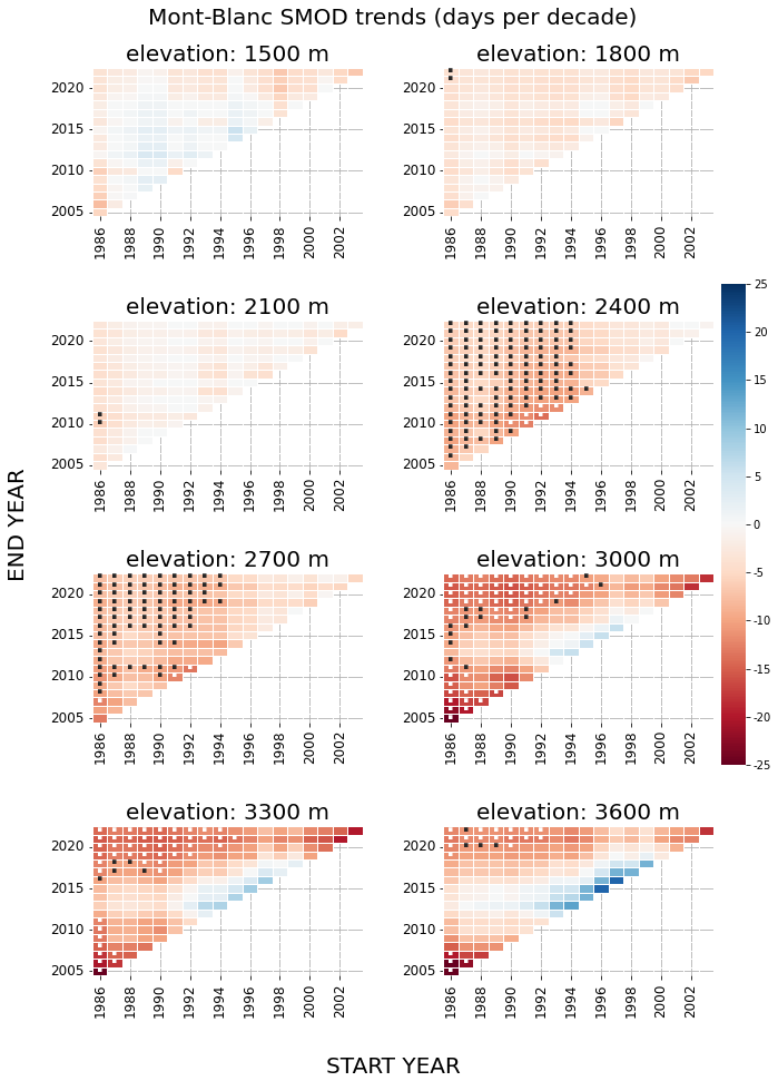
Figure 10 Mont Blanc massif (French Alps). Results of the Mann–Kendall test over the trend of the SMOD median of each elevation band (± 150) are filtered for NOBS_min ≥ 10 and applied to all possible combinations of start and end dates involving at least 20 years for HYs 1986 to 2022. Colors indicate the SMOD trend in days per decade, and dots indicate statistically significant trends (p value < 0.05).

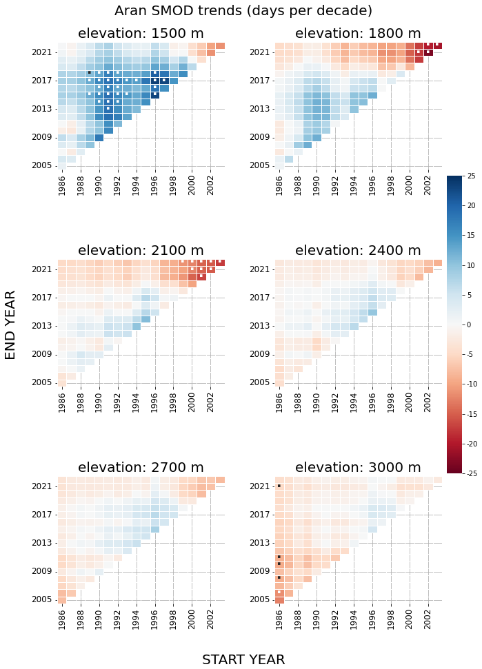
Figure 11 Aran massif (Pyrenees). Results of the Mann–Kendall test over the trend of the SMOD median of each elevation band (± 150) are filtered for NOBS_min ≥ 10 and applied to all possible combinations of start and end dates involving at least 20 years for HYs 1986 to 2022. Colors indicate the SMOD trend in days per decade, and dots indicate statistically significant trends (p value < 0.05).

We found that the trends were sensitive to the period of computation (start and end years), but the impact was more evident in the Pyrenees. Here we show Mont Blanc in the French Alps (Fig. 10) and the Aran massif in the Pyrenees (Fig. 11). In the Mont Blanc massif, the trends can become positive (non-significant) for periods starting between 1992 and 1999 and ending between 2011 and 2018. In the Aran massif, at 1500 and 1800 m, we find positive (significant) trends for periods ending before 2020. Above 1800 m, and similarly to the Alps, we found an interval of (non-significant) positive trends with starting years near 1995.

5 Discussion

5.1 Snow melt-out day errors

The satellite SMOD was in relatively good agreement with the in situ SMOD, with half of the ΔSMOD below 11 d. We found an overestimation of the SMOD that was similar to previous works using MODIS data. Dietz et al. (2012) observed SMOD overestimations that were larger than underestimations from daily MODIS time series over Europe, and the same was observed over the Tian Shan (Wang and Xie, 2009). Notarnicola (2020) also reported positive biases at low and middle latitudes (including the Alps and Pyrenees) while showing negative biases at high latitudes, similarly to Lindsay et al. (2015), who found negative biases over Alaska. The main hypotheses mentioned to explain the biases were the uncertainties caused by cloud pixels delaying the observation of snow or no-snow days and the impact of MODIS medium-resolution pixels covering heterogenous mountain topography and snow–no-snow transition areas as well as forested and urban areas close to the ground stations used for validation. Positive biases were also found over European mountains using lower resolutions (Metsämäki et al., 2018). Their histogram of ΔSMOD values between 0.1° resolution optical images and 25 km microwave images was distributed similarly (a mode at zero and positive values reaching up to 100 d) to the one shown above with a similar RMSE.

The French Alps showed no negative or positive bias. In contrast, the French Pyrenees showed positive biases at elevation bands from 1500 to 2100 m and a smaller negative bias at 2400 m. Results are more uncertain on the Spanish side of the Pyrenees, where only four stations were available. While the in situ data in the 2400 m elevation band were limited and should be treated with caution, the Alps and Pyrenees data indicate that the SMOD error is reduced at higher elevations. To determine whether the changes in bias with elevation could be partially explained by variations in TCD, we calculated the correlation between TCD and elevation for all pixels with elevations greater than 1200 m and TCD values between 1 and 50. We found no correlation (−0.01) between the two. Our hypothesis for the lower performances over the Pyrenees compared to the Alps is that the mountain range suffers from both a reduced number of high-elevation stations and a smaller proportion of NOBS above or equal to 25. The proportions of NOBS ≥ 25 are 77.4 % for 1201 values over the Alps and 61 % for 308 values over the Pyrenees (Fig. 12).

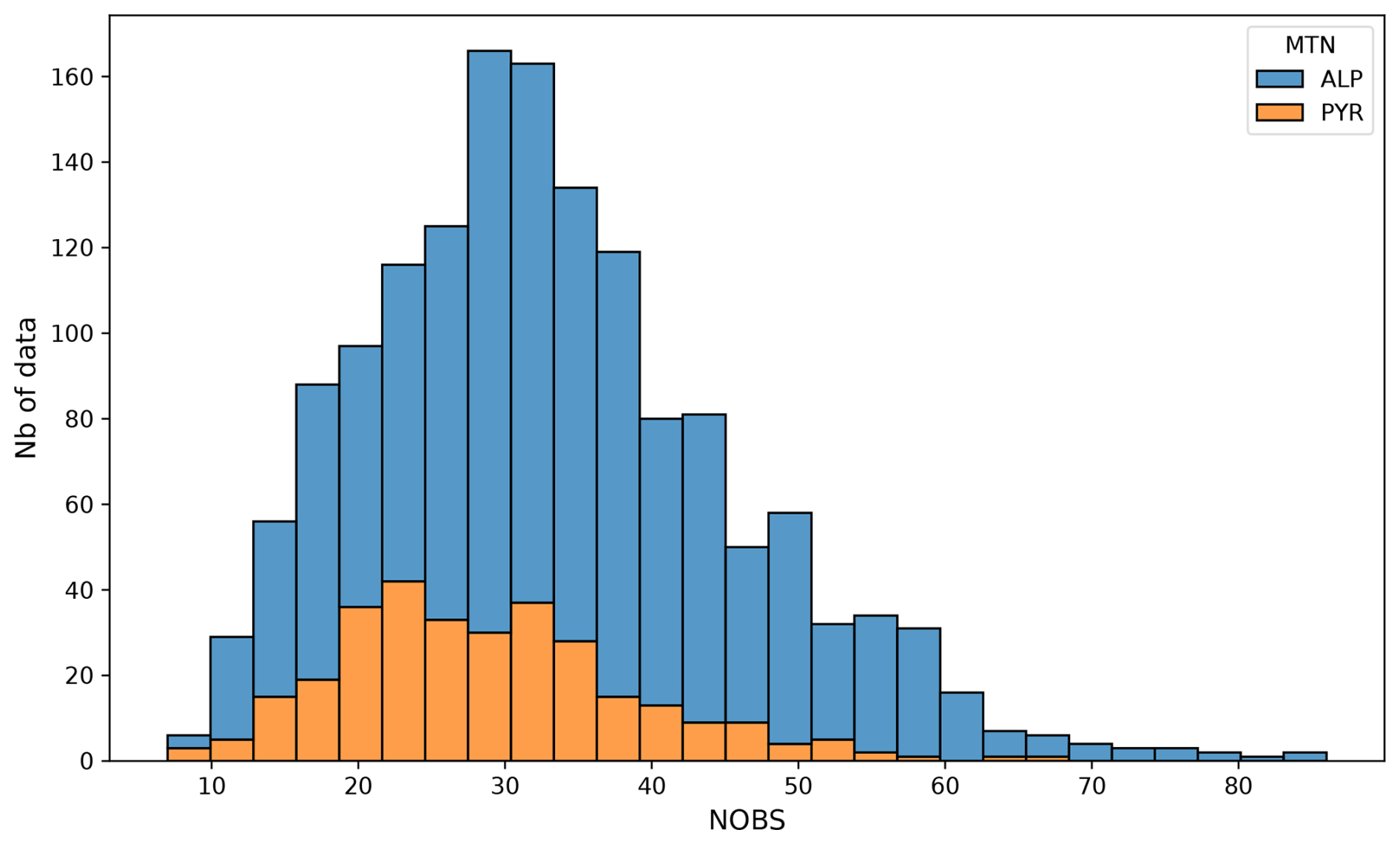
Figure 12 Distribution of NOBS values between the stations of the Alps and the stations of the Pyrenees.

We note that the errors discussed above were obtained at the pixel level. Hence, they represent an upper bound of the error on the SMOD values that were eventually used for the trend analysis, since we performed a spatial aggregation of at least 1000 pixel values before computing the trends (Sect. 3.3).

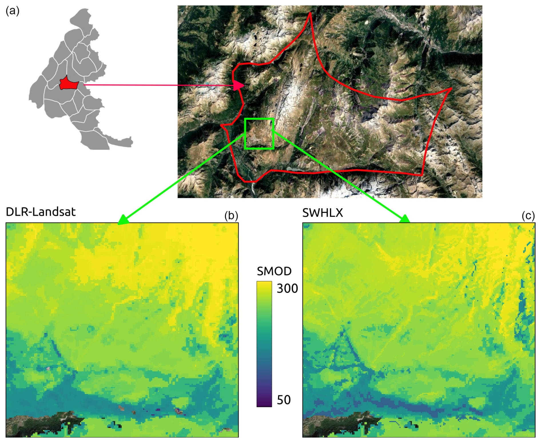
Figure 13 Alpe d'Huez, hydrological year 1997: comparison between the 20 m resolution SMOD maps from DLR-Landsat (b) and SWHLX (c).

SWH enables us to partly overcome the lack of cloud-free observations when using Landsat data only, especially in areas where Landsat revisit times are long (Barrou Dumont et al., 2023). SMOD images can also be computed at 20 m instead of 30 m, and the enhanced spatial–temporal resolution of a combined SWH–Landsat dataset results in a SMOD image with more spatial details than a SMOD image from Landsat only (Fig. 13). However, it should be noted that this benefit is spatially variable due to the on-demand acquisition mode of SPOT satellites. In the Pyrenees, for example, we observed that SWH acquisitions were more frequent over French territory.

5.2 Snow melt-out day trends

A low number of statistically significant trends, together with the presence of positive trends at elevation bands of 1500 and 2100 m for shorter uninterrupted periods, was also observed in the Pyrenees by López-Moreno et al. (2020) between 1986 and 2018. They specifically found an increase in the snow duration at the Aspe Ossau massif and increases in the snow depths at Navarra at 1500 m and Luchonnais at 2100 m. These observations coincide for Aspe Ossau and Navarra, with satellite-based positive SMOD trends calculated for periods of 20 years or more over the same areas (see Fig. D4 in the Appendix). They do not coincide with the satellite-based neutral and negative trends calculated at Luchonnais at 2100 m.

Notarnicola (2022) found, for the 1982–2020 period over the Pyrenees, a small (< 5 %) non-significant increase in the SCA between December and May that is consistent with the positive trends of SMOD seen at low elevations. The overall absence of significant trends over the Pyrenees for the 1986–2023 period can be explained by the influence of the Mediterranean climate on the southern and eastern Pyrenees, which is characterized by high interannual variability. Despite a well-identified warming trend (OPCC-CTP, 2018), natural climate variability and in particular winter precipitation variability can mask the effect of warming on snow cover duration. In particular, the variability in snowfall is partly controlled by the North Atlantic Oscillation at decadal timescales (Lemus-Canovas et al., 2024).

We found mostly negative SMOD trends in the French Alps, ranging between −3 and −10 d per decade, in agreement with previous studies in the European Alps over similar time periods using in situ data (Klein et al., 2016; Matiu et al., 2021), reanalyses (Monteiro and Morin, 2023), or satellite observations (Notarnicola, 2022).

We found significant trends at high elevations, unlike previous works using coarser-resolution remote sensing data (Hüsler et al., 2014), which highlights the value of high-resolution remote sensing in this scope. In particular, trends are significant and strongly negative for elevations above 2100 m in the Mont Blanc massif, which is consistent with previous work (CREA, 2024). Negative trends are stronger in the northern Alps at 1500 m and in the southern Alps at 2100 m. This was also observed by Durand et al. (2009) for the 1958–2005 period. This spatial gradient is consistent with the Alps' climate, as seasonal snow is found at higher elevations in the southern Alps. Our dataset also shows that trends in the Mont Blanc massif were positive (non-significant) for periods starting between 1992 and 1999 and ending between 2011 and 2018 and negative for periods starting in 2000 and after. This illustrates the importance of using remote sensing time series spanning multiple decades to draw robust conclusions regarding snow cover trends in European mountains. However, our dataset still remains too small to characterize some multi-decadal climatic variations. In particular, in the Alps, Durand et al. (2009) and Marty (2008) hypothesized the presence of a break year in the mid-1980s marking an abrupt transition between two periods, with the first having significantly higher snow cover duration and snow depth than the second. A similar conclusion was drawn from recent reanalyses (Monteiro and Morin, 2023; Beaumet et al., 2021). Our study period started either in or after this break year and thus does not capture this transition.

6 Conclusions

The objective of this work was to analyse SMOD trends in the French Alps and Pyrenees as well as their spatial variability. We combined different collections of SPOT, Landsat, and Sentinel-2 products to create an unprecedented time series of high-resolution snow cover products. We used this dataset to compute 20 m resolution SMOD images for 37 hydrological years from September 1986 to August 2023. Despite numerous challenges in terms of image processing, temporal gap filling, and data fusion, the estimated SMODs were in agreement with SMOD data obtained from the in situ snow depth time series. This allowed us to estimate SMOD trends from HYs 1986 to 2022 for different regions by topographical class (elevation, aspect, and DAH).

We found a general reduction in the SMOD, revealing a widespread trend towards an earlier disappearance of the snow cover, with an average reduction of 5.78 d per decade over the French Alps and a standard deviation of 4.88 d per decade. Over the Pyrenees, we found an average reduction of 4.33 d per decade with a standard deviation of 4.64 d per decade. The results were less homogeneous in the Pyrenees, where we also found a few positive trends at 1500 m, but these trends were not robust to changing periods. Overall, the results were consistent with previous studies over these mountain ranges. However, the studied period might not be long enough to detect trends in areas of short-lived snow cover (“marginal snowpacks”, López-Moreno et al., 2024) and areas under the influence of the Mediterranean climate. Other points of interest are the following:

• In the French Alps, there is a transition of the statistically significant negative trends from the north at 1500 m to the south at 2100 m. This may reflect the climatic gradient like the increasing elevation of the 0° isotherm.

• There is a strong correlation between the pixel-wise SMOD uncertainties and the NOBS when the latter is under 26, and a linear function of NOBS could be used to model the SMOD error and generate a pixel-wise quality mask accompanying the SMOD products for more local applications.

• The 20 m resolution pixels give enough data points to build SMOD medians robust to the uncertainties from the lower NOBS and to build significant trends from deeper levels of stratification (massif, elevation, aspect, and DAH).

Other snow phenology variables like the snow onset day or the snow cover duration could also be estimated using the same dataset. However, the snow onset day is probably subject to higher uncertainty due to the presence of clouds when the snow season begins. Ultimately, the snow cover products (Level 2B) could be used to evaluate and/or constrain climatological reanalyses of the snow cover through data assimilation in combination with in situ data and existing meteorological models. For that purpose, the error observation could be estimated from our results as a function of the number of available observations. Finally, the same satellite data could be used to study vegetation trends with the near-infrared band of the images.

Appendix A: Snow and cloud classification in historical SPOT images

Barrou Dumont et al. (2024) developed an emulator of SPOT images from Sentinel-2 Level-1C images to train a statistical model of snow and cloud classification in SPOT images. Indeed, the emulation approach allowed pairing of a pseudo-SPOT image with a Sentinel-2 Level-2B product that provides the labels (snow, no snow, and cloud) required for the training. The trained model was a U-Net convolutional neural network (Ronneberger et al., 2015), which yielded high precision in detecting snow and minimal false snow pixel identification. However, haze and highly transparent and semi-transparent clouds could be detected in Sentinel-2 images thanks to their higher number of spectral bands and their radiometric quality. These clouds were almost invisible in pseudo-SPOT images, creating “false” clouds in the training dataset and causing an overestimation of cloud pixels by U-Net.

To solve this issue, we filtered the cloud pixels from the training data according to how they were detected. The cloud mask in the Level-2B products was generated with the MAJA software, which provides information on the way in which a cloud pixel was detected (Hagolle et al., 2017). In particular, one way of detecting clouds was a combination of pixel-wise mono-temporal reflectance thresholds in the blue, red, NIR, and SWIR bands. Cloud pixels detected with the mono-temporal threshold were certain to also be visible in the SPOT 1–5 instruments. Keeping only these cloud pixels reduced the number of misleading labels.

Cloud shadow pixels were also removed from the training to capitalize on the observation of Barrou Dumont et al. (2024) that U-Net was able to detect snow in less illuminated areas.

We also changed the number of times the training dataset was run through the neural network (number of epochs). In Barrou Dumont et al. (2024), this starts with short parallel preliminary training for 40 epochs to look for the best weight initialization where U-Net can converge to a state of minimum loss, and it continues with more intensive training for 200 epochs. One solution to ensure that U-Net converges to the state of minimum loss afforded by its architecture and the training data is to remove the limit on the number of epochs and to stop each training step when U-Net stops improving for a given number of epochs (40 for preliminary training, 200 for intensive training).

One U-Net model was trained for each of the five SPOT instruments and by mountain range (French Alps and Pyrenees), i.e. a total of 10 models. The SWIR band in SPOT 4 HRVIR and SPOT 5 HRG was emulated and included as an additional input in the training of the SPOT 4 and SPOT 5 models. For the Pyrenees, Sentinel-2 training images were selected randomly using the same methodology as Barrou Dumont et al. (2024). For the French Alps, the Sentinel-2 tiles are 31TGM, 31TGL, 31TGK, 31TGJ, 32TLS, 32TLR, 32TLQ, and 32TLP, and only complete images (data on the image edges) were selected (the complete images correspond to a relative orbit number of 108 for the French Alps). This represented totals of 46 images over the Pyrenees and 92 images over the French Alps. Inference was then applied to each model to extract snow and cloud cover maps from the entire SPOT dataset. Because the inference of a pixel depends on the value of the surrounding pixels, we masked pixels too close (2000 m) to the border of the image or too close to no-data areas of the image to ensure equal performance of the neural network across the data.

Appendix B: Statistical metrics

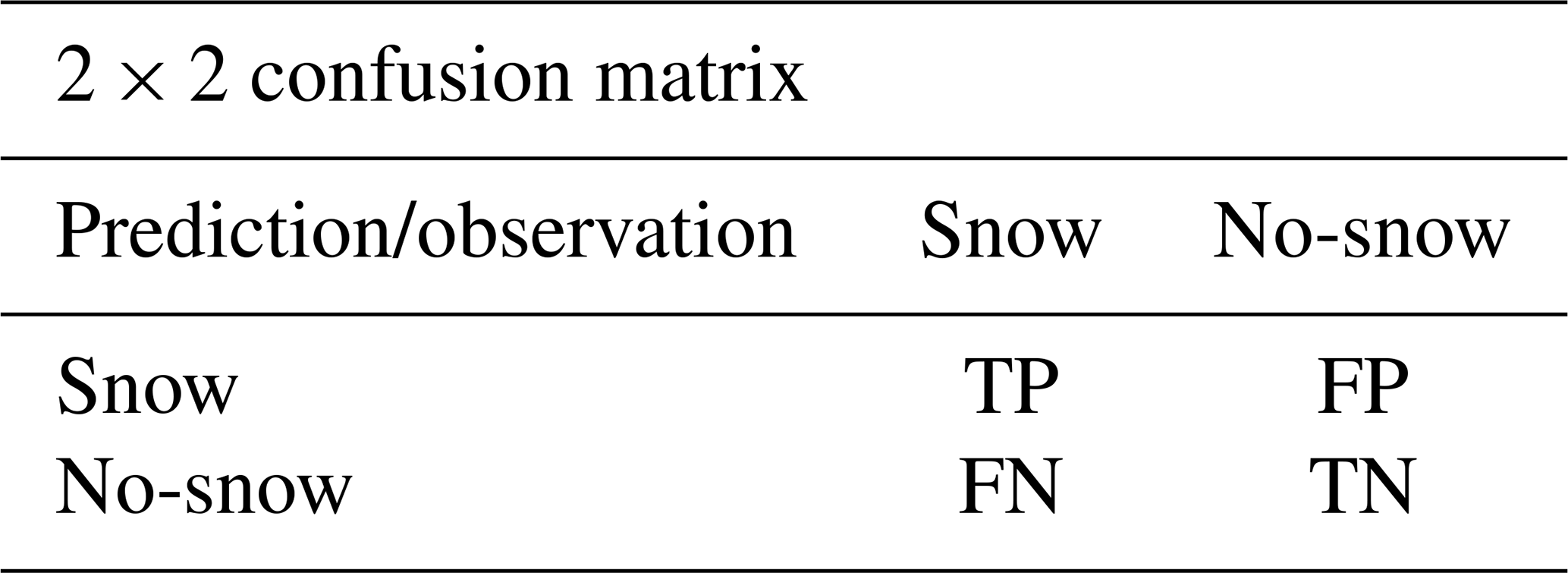
The confusion matrix aggregates the different combinations of predicted and observed (e.g. ground truth) values. When the prediction is a binary choice (snow or snow-free), the correct prediction of the value of interest (snow) is called a true positive (TP) and its incorrect prediction is called a false positive (FP). The correct prediction of the alternative value (snow-free) is called a true negative (TN), and its incorrect prediction is called a false negative (FN) (Table B1). These metrics can then be used to calculate the precision (which is the fraction of correct predictions of snow), the recall (which is the fraction of observed snow which has been retrieved), and the F1 score (which is the harmonic mean of the precision and the recall) (Eq. B1). The F1 score is particularly well adapted to evaluating a classifier over an unbalanced dataset, which is to be expected when using satellite images of mountain ranges.

Table B1 Confusion matrix between predictions and observations of the snow and no-snow classes.

$$\begin{array}{}\text{(B1)}& \begin{array}{rl}{\text{Precision}}_{\text{snow}}& ={\displaystyle \frac{\text{TP}}{\text{TP}+\text{FP}}}\\ {\text{Recall}}_{\text{snow}}& ={\displaystyle \frac{\text{TP}}{\text{TP}+\text{FN}}}\\ {\text{F1}}_{\text{snow}}& ={\displaystyle \frac{\mathrm{2}\times {\text{Precision}}_{\text{snow}}\times {\text{Recall}}_{\text{snow}}}{{\text{Precision}}_{\text{snow}}+{\text{Recall}}_{\text{snow}}}}\end{array}\end{array}$$

Common metrics for the evaluation of continual outputs like the SMOD include the RMSE, which is the quadratic mean of the difference between predicted and observed values. Because the errors are squared, the RMSE is sensitive to outliers, as even a few large errors can raise its value significantly. The MAE is the median of the differences where the sign of the difference is ignored to avoid cancellations between positive and negative errors. In contrast to the RMSE, the MAE is not affected by outliers. The IQR is the difference between the 75th and 25th percentiles of a dataset. The RMSE is expressed as

$$\begin{array}{}\text{(B2)}& \text{RMSE}(y,\widehat{y})=\sqrt{{\displaystyle \frac{{\sum }_{i=\mathrm{0}}^{N-\mathrm{1}}(y_i-{\widehat{y}}_i{)}^{\mathrm{2}}}{N}}},\end{array}$$

with i the value number, N the number of values, y the predicted value, and $\widehat{y}$ the observed value.

Appendix C: Agreements between satellite products

C1 Evaluation of SWH and DLR-Landsat agreement

To assess the differences and similarities between the SWH and DLR-Landsat datasets, pairs of overlapping SPOT and Landsat Level-2B products were assembled from same-day acquisitions and were re-projected to 30 m resolution (using nearest-neighbour resampling). A comparison of the two datasets was first made qualitatively with a visual comparison of the Level-2B products between the SPOT instruments HRV, HRVIR, and HGR and the Landsat instruments TM, ETM+, and OLI in both cloudy and cloud-free contexts. A quantitative assessment was also conducted by computing a contingency matrix of the labels, excluding pixels under the water and glacier masks and with TCD > 50 %. The comparison was restricted to the snow and no-snow labels, excluding cloud pixels, because cloud cover can change in the time interval between two same-day acquisitions. Landsat Level-2B products have a shadowed area and water body label, which was merged with the cloud label as no-data values. From the contingency matrix between SWH and DLR-Landsat data, we derived the F1, recall, and precision scores of SWH (see Appendix B). The use of these metrics typically implies that a predicted dataset is compared to a reference dataset, but, in this case, they served to study the similarities between both datasets.

Table C1 Distribution of snow and cloud labels among the SWH and DLR-Landsat pairs.

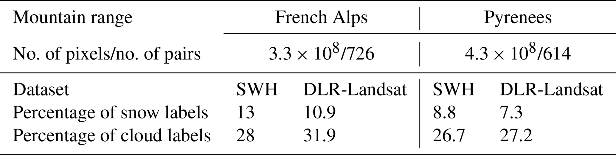
We assembled 1340 pairs of Landsat (DLR-Landsat) and SPOT (SWH) products acquired on the same day. There were more snow pixels and fewer cloud pixels from SWH than from DLR-Landsat (Table C1), and the differences were larger in the Alps than in the Pyrenees. When cross-masking cloud labels from both datasets, both products had high agreement with each other, with a snow recall of 0.99 and a snow precision of 0.98 for an F1 score of 0.98. Visual comparisons can be found in the Appendix (Figs. C1–C3). They illustrate the overall good agreement between both datasets despite the different methods to generate them as well as the differences in the classifications. Border areas between the snow-covered and no-snow regions contained ambiguous pixels that were harder to classify correctly (Fig. C1). The DLR-Landsat method hid these pixels under a cloud label, avoiding the risk of generating false snow positives. Inversely, SWH 2B products classified those pixels as either snow or no-snow. Other noticeable differences between DLR-Landsat and SWH were that SWH overestimated the sizes of existing clouds (Fig. C2) and that shadowed snow areas were misclassified as clouds with the DLR-Landsat approach (Fig. C3).

C2 Evaluation of Sentinel-2 and Landsat 8 agreement in the Theia dataset

The same quantitative evaluation of Appendix C1 was applied over eight pairs of snow products from Landsat 8 (L8) and Sentinel-2 (S2). These image pairs were acquired on the same day between November 2017 and June 2018, covering areas in the Alps and Pyrenees. From a dataset of 7.7 × 10⁷ pixels, 34 % and 31 % were classified as snow by S2 and L8, respectively; 96 % of the L8 snow pixels were detected with S2, and 89 % of the S2 snow pixels were detected with L8, for an F1 score of 0.92 between the two products.

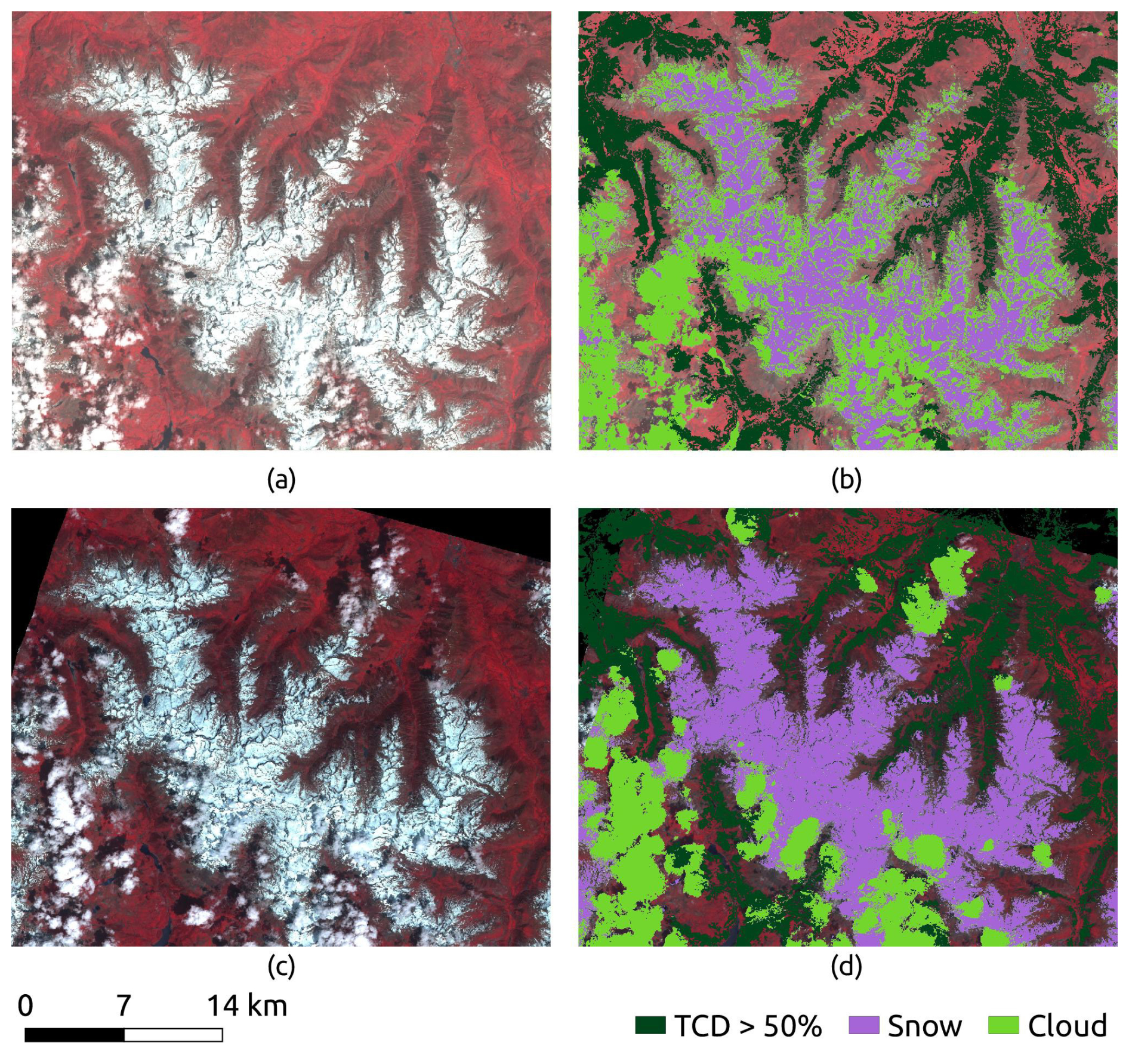
Figure C1 The Pyrenees on 25 May 1987: 30 km × 30 km scene with (a) the Landsat 5 TM image (green, red, and SWIR), (b) the DLR-Landsat 2B product, (c) the SPOT 1 HRV image (green, red, and NIR), and (d) the SWH 2B product.

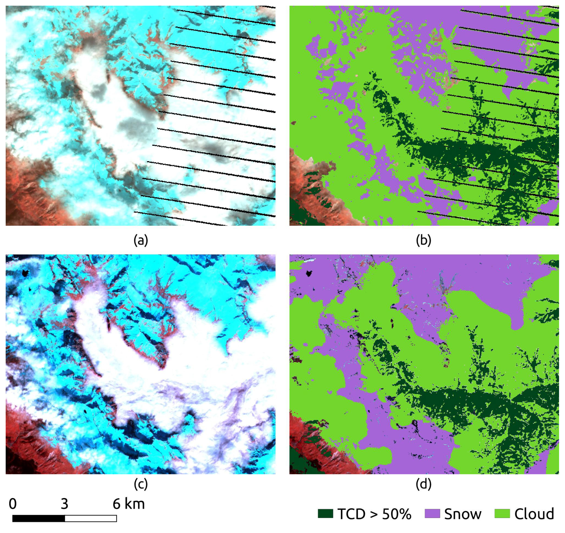
Figure C2 The Alps on 13 October 2005: 12 km × 12 km scene with (a) the Landsat 7 ETM+ image (green, red, and SWIR), (b) the DLR-Landsat 2B product, (c) the SPOT 4 HRVIR image (green, red, and SWIR), and (d) the SWH 2B product.

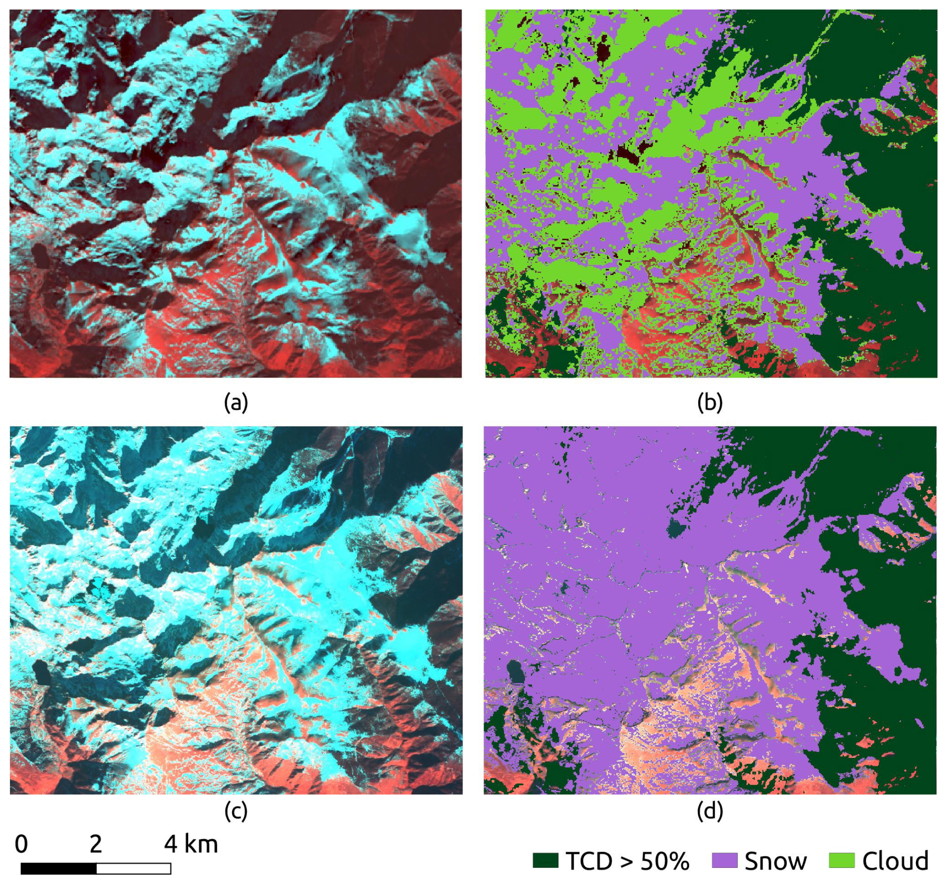
Figure C3 The Alps on 3 December 2013: 12 km × 12 km scene with (a) the Landsat 8 OLI image (green, red, and SWIR), (b) the DLR-Landsat 2B product, (c) the SPOT 5 HRG image (green, red, and SWIR), and (d) the SWH 2B product.

Appendix D: Additional figures

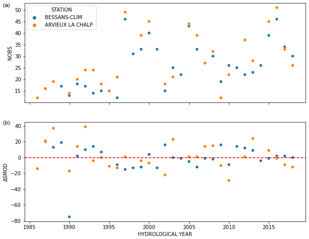
Figure D1 Yearly NOBS (a) and ΔSMOD (b) values from the two stations which only recorded observed snowmelt dates (not gap-filled) for the entirety of the study period.

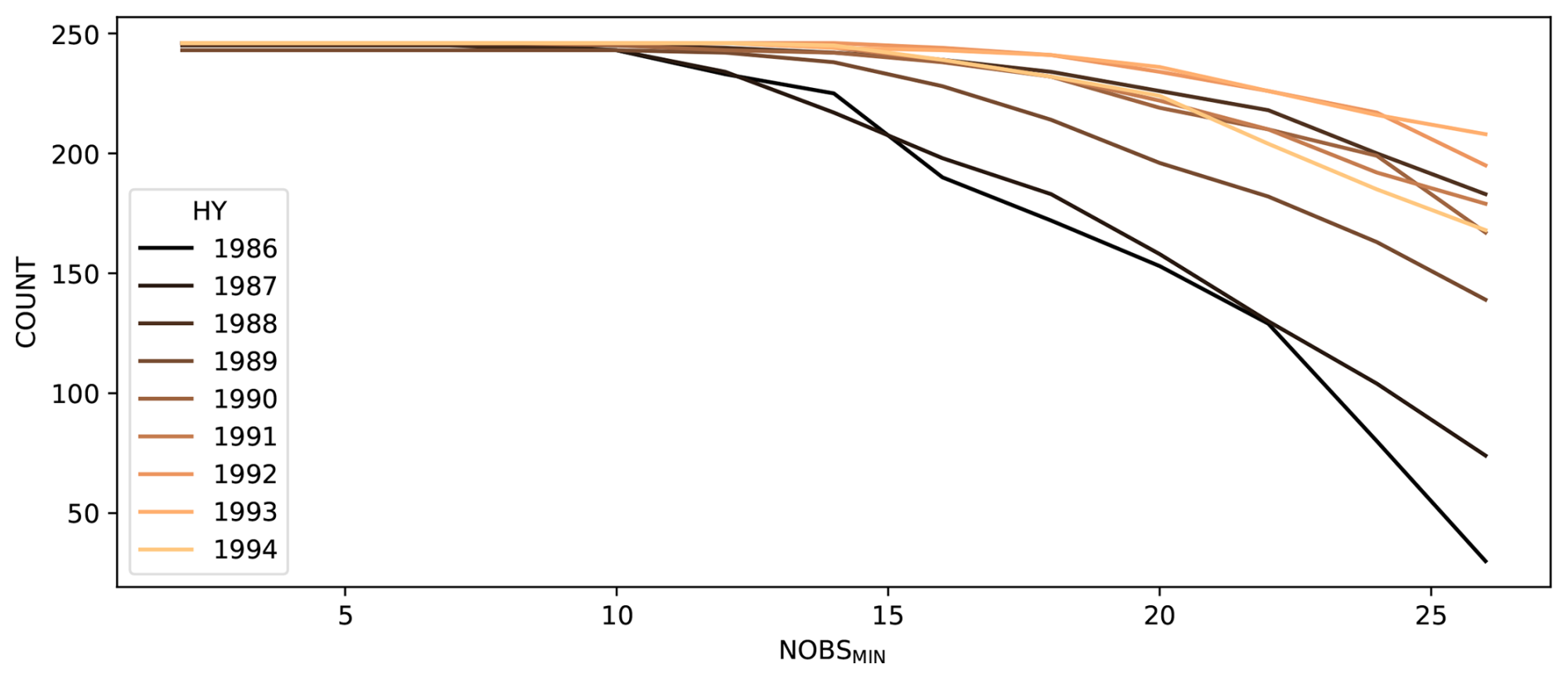
Figure D2 Number of available SMOD medians from every combination of massif and elevation band as a function of NOBS_min for all HYs before 1995. A loss of data was observed for NOBS_min thresholds above 10, with a stronger effect before 1989. For later periods, a NOBS_min of 26 still allows us to maintain most of the available combinations of massif and elevation band. For 1986, a NOBS_min of 26 reduces the available combinations of massif and elevation band to 28.

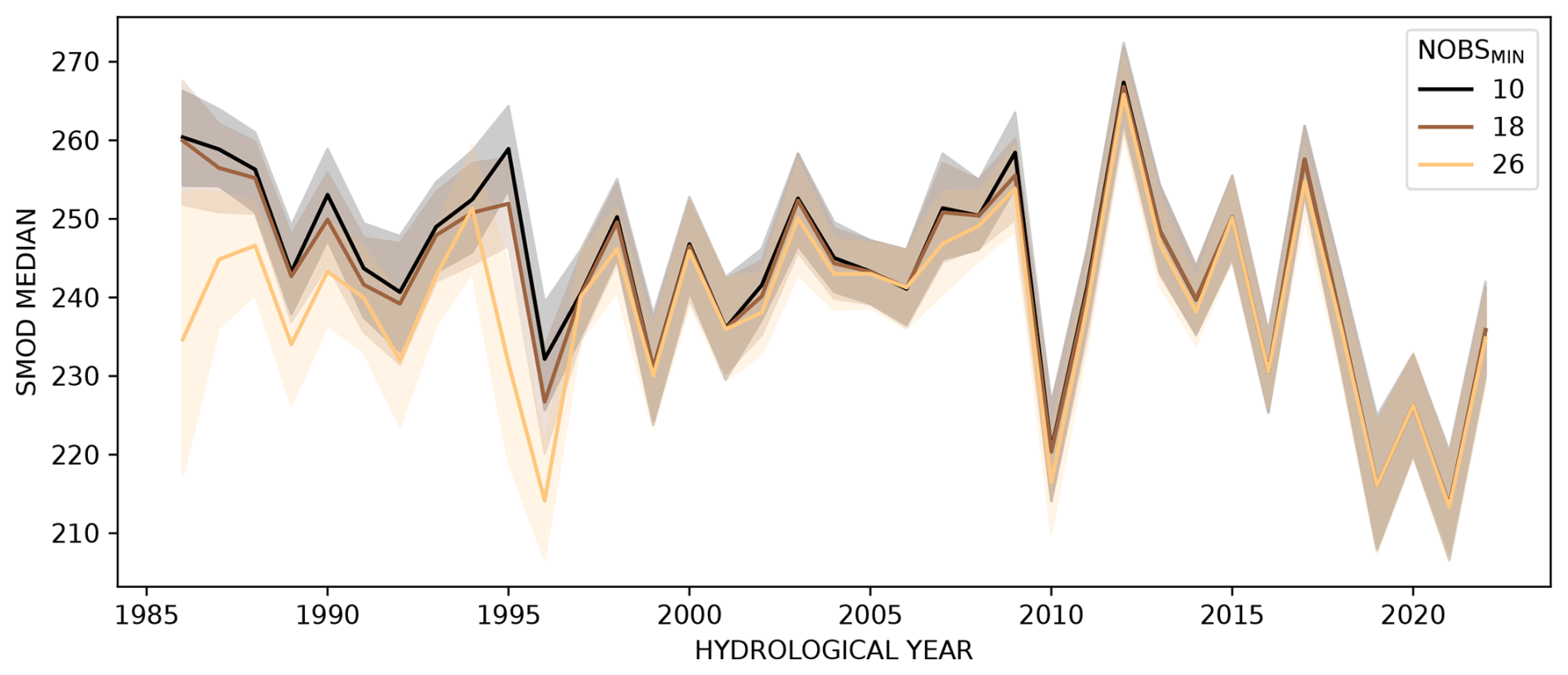
Figure D3 Yearly average of the SMOD medians from each combination of massif and elevation band, with a confidence interval of 95 %, for NOBS_min values of 10, 18, and 26. The distribution is robust to NOBS_min, except for earlier years at a NOBS_min value of 26, due to the significant reduction in the available combinations.

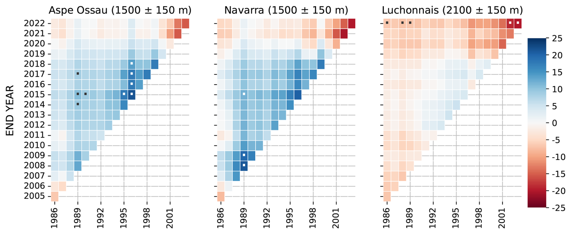
Figure D4 Massifs Aspe Ossau (1500 m), Navarra (1500 m), and Luchonnais (2100 m). Results of the Mann–Kendall test over the trend of the SMOD median are filtered for NOBS_min ≥ 10 and applied to all possible combinations of start and end dates involving at least 20 years for HYs 1986 to 2022. Colors indicate the SMOD trend in days per decade, and dots indicate statistically significant trends (p value < 0.05).