Role of elevation feedbacks and ice sheet–climate interactions on future Greenland ice sheet melt

The Greenland ice sheet (GrIS) stores freshwater equal to more than 7 m of potential sea level rise (SLR) and strongly interacts with the Arctic, North Atlantic and global climate. Over the last few decades, the ice sheet has been losing mass at a rate that is projected to increase. Interactions between the GrIS and the climate have the potential to amplify or reduce GrIS mass balance responses to ongoing and projected warming. Here, we investigate the impact of ice sheet–climate interactions on the climate and mass balance of the GrIS using the Community Ice Sheet Model version 2 (CISM2) coupled with the Community Earth System Model version 2 (CESM2). To this end, we compare two idealized multi-century simulations with a non-evolving and evolving ice sheet topography in which we apply an annual 1 % increase in CO₂ concentrations, starting from pre-industrial (PI) until stabilization at 4×PI CO₂ concentrations (4×CO₂). By comparing the one- and two-way coupled simulations, we find significant changes in atmospheric blocking, precipitation and cloud formation over Greenland as the GrIS topography evolves, acting as negative feedbacks on mass loss. We also attribute part of the overestimation of mass loss in the one-way coupled simulation to an overestimation of melt in the ablation area caused by the use of a uniform temperature lapse rate to reflect the elevation differences between the atmospheric and ice sheet grids. Furthermore, we investigate ice sheet–climate interactions in a simulation branched in year 350 from our two-way coupled simulation in which we annually reduce atmospheric CO₂ by 5 % until PI concentrations are reached. During the 350-year 4×CO₂ forcing period, the ice sheet loses a total mass of 1.1 m sea level equivalent, and part of its margins retreat landward. When the PI CO₂ concentration is restored, melt decreases rapidly, leading to a small positive surface mass balance. Combined with the strongly reduced ice discharge resulting from the widespread retreat of the ice sheet margin, this halts GrIS mass loss despite a remaining global warming of 2 K. The GrIS, Arctic and North Atlantic strongly interact, causing a complex transitional phase towards a colder climate during the century following the CO₂ reduction. Elevated atmospheric temperatures, larger ocean heat transport and deteriorated state of the snowpack, compared to the initial pre-industrial state, result in limited regrowth of the ice sheet under reintroduced PI CO₂ conditions.

1 Introduction

Over the past century, the rate of global mean sea level rise (SLR) has exceeded any previous period (Fox-Kemper et al., 2021) and has been accelerating since the late 1960s (Dangendorf et al., 2019). Melt of the Greenland ice sheet (GrIS), storing more than 7 m of potential SLR (Morlighem et al., 2017), has caused ∼18 % of contemporary SLR (Otosaka et al., 2023), and its contribution is expected to increase (Bamber et al., 2019; Goelzer et al., 2020). The Sixth Assessment Report (AR6) of the Intergovernmental Panel on Climate Change (IPCC; Fox-Kemper et al., 2021) attributes the largest uncertainties in future sea level rise to the Greenland and Antarctic ice sheets. Therefore, understanding the physical drivers for GrIS mass loss and adequate numerical modeling of their effects on the GrIS mass balance are crucial to provide reliable projections of global and regional SLR.

Contemporary climate change, caused by anthropogenic greenhouse gas emissions (Jones et al., 2013; Ribes and Terray, 2013), influences surface mass processes over the GrIS in connection with rising Northern Hemisphere summer temperatures (Hanna et al., 2008). Moreover, changes in the GrIS have the potential to influence local and global climate (Vizcaíno, 2014) because of their interaction with key components of the Earth system through various processes and feedbacks (Fyke et al., 2018). Important feedback mechanisms include the positive melt–elevation feedback (Edwards et al., 2014; Vizcaíno, 2014; Fyke et al., 2018), the positive melt–albedo feedback (Box et al., 2012; Fyke et al., 2018) and the negative melt–discharge feedback (Goelzer et al., 2013; Fürst et al., 2015; Vizcaíno et al., 2015). The strong coupling between the GrIS and the atmosphere potentially influences atmospheric circulation and precipitation patterns (Ridley et al., 2005; Fyke et al., 2018). The GrIS heavily interacts with the ocean, as the North Atlantic Meridional Overturning Circulation (NAMOC) influences GrIS temperatures, while freshwater influxes as a result of GrIS mass loss can influence the strength of the NAMOC (Driesschaert et al., 2007). Accounting for these interactions between the Earth system and the GrIS in climate models is critical to obtain reliable projections of SLR and GrIS evolution (Vizcaíno, 2014; Fyke et al., 2018). It has been shown that one-way coupled simulations, in which changes in the state of the GrIS are not communicated to the Earth system model (ESM), overestimate multi-centennial GrIS mass loss (Ridley et al., 2005; Gregory et al., 2020) as several feedbacks are not represented in these simulations. Ridley et al. (2005) identify more precipitation and less melt in a two-way coupled simulation, in which the GrIS is an interactive component within the Earth system model and attribute this to a change in atmospheric circulation patterns over Greenland. In contrast, Gregory et al. (2020) attribute the reduced mass loss to an increase in cloud fraction, causing an increase in reflected shortwave radiation. Next to that, they find a land-inward migration of precipitation patterns caused by topographic changes.

Considering that by 2022, global temperatures have increased by 1.09 °C (0.95–1.20) compared to the 1850–1900 baseline (Gulev et al., 2023), reaching the 1.5 °C goal of the Paris Agreement is becoming less likely over time (Matthews and Wynes, 2022). The rapidly increasing global temperatures call for the investigation of “overshoot” scenarios in which this temperature threshold is surpassed. Such an overshoot could have important implications for the evolution of the GrIS-induced SLR as global mean sea level (GMSL) could rise substantially under the higher temperatures during such an overshoot period (Schwinger et al., 2022). Due to the nonlinear and tipping nature of the Earth system, there might be non-reversible effects associated with an overshoot scenario. Consequently, investigating the response of the GrIS to these kinds of scenarios is of great importance for assessing the implications of following an overshoot pathway. Previous work (Ridley et al., 2010; Robinson et al., 2012; Gregory et al., 2020; Bochow et al., 2023) shows that temperature and volume thresholds for irreversible GrIS mass loss might exist. These model-based studies show that if temperature overshoots are limited and the ice sheet does not lose a critical ice volume, mass loss can be halted or might even be reversible. However, a thorough model-based assessment of the role played by ice sheet–climate feedbacks in the reversibility of enhanced deglaciation rates is currently lacking. As ice sheet–climate interactions could potentially accelerate or slow down the changes in GMSL caused by the response of the GrIS to CO₂ reduction, it is important to account for them to obtain a reliable projection of SLR in an overshoot scenario.

Considering these ice sheet–climate feedbacks and interactions can be done by coupling an ice sheet model with an Earth system model or a regional climate model. Over the past few years, there has been a lot of development regarding these kinds of models (e.g., Ridley et al., 2005; Gregory et al., 2020; Madsen et al., 2022; Delhasse, 2024).

In this paper, we use a coupled ice sheet–Earth system model setup to assess the impact of ice sheet-climate interactions on the mass balance of the GrIS. We evaluate the impact of these interactions under an idealized extreme warming scenario, in which we annually increase atmospheric CO₂ by 1 % from pre-industrial (PI) concentrations until 4 times the PI CO₂. We begin by comparing two simulations with this idealized forcing, of which one allows for changes in the GrIS topography to be communicated to the Earth system model (two-way coupling) and one does not (one-way coupling). We then branch a third simulation from the two-way coupled simulation in year 350 (i.e., after 2 centuries of sustained 4×CO₂ conditions), where we bring back PI CO₂ concentrations with an annual 5 % decrease (covering 27 years), to assess the impact of ice sheet–climate interactions on the response of GrIS deglaciation rates to CO₂ reduction.

In Sect. 2, we describe the coupled model setup, the simulations conducted and our analysis methods. Section 3 assesses the influence of the coupling on the simulated GrIS mass loss, and Sect. 4 gives an overview of the most important elevation feedbacks that influence the GrIS mass balance. In Sect. 5, we investigate other ice sheet–climate interactions and address GrIS mass balance response resulting from the reintroduction of PI CO₂ conditions. We discuss our results and draw conclusions in Sects. 6 and 7, respectively.

2 Method

2.1 Model description

We use the Community Earth System Model version 2 (CESM2; Danabasoglu et al., 2020) and the Community Ice Sheet Model version 2 (CISM2; Lipscomb et al., 2019), which are coupled to account for an evolving ice sheet. CESM2 is a state-of-the-art community-developed ESM, developed by the US National Science Foundation (NSF) National Center for Atmospheric Research (NCAR). CESM2 can produce a realistic surface mass balance (SMB; van Kampenhout et al., 2020) over the GrIS using a surface energy balance (SEB) scheme. CESM2 consists of different component models for land and land biochemistry, atmosphere, river runoff, surface waves, ocean and marine biochemistry, sea ice, and land ice, which are coupled to exchange states and fluxes via a hub-and-spoke architecture (Danabasoglu et al., 2020).

The atmosphere model is the Community Atmosphere Model version 6 (CAM6; Gettelman et al., 2019), which runs on a nominal 1° (1.25° in longitude and 0.9° in latitude) grid and has 32 vertical levels. The Community Land Model version 5 (CLM5; Lawrence et al., 2019) shares the horizontal grid of the atmosphere model. In this land model, every grid cell is divided into one or multiple fractions of land units, which can be glacier, lake, wetland, urban, vegetation and crop surface. Calculations are carried out separately over the different land units. The model has a fixed number of vertical layers for the soil, whereas there is a variable number of layers for snow and firn, with a maximum snow depth of 10 m water equivalent (w.e.). The model allows for the compaction of snow into firn. Accumulation of snow over 10 $\mathrm{m}\mathrm{w}.\mathrm{e}.$ in a grid cell is transferred as positive SMB to the ice sheet model. If snow and firn are melted away, further melt of ice is transferred as negative SMB (ice ablation) to the ice sheet model. Changes within the 10 $\mathrm{m}\mathrm{w}.\mathrm{e}.$ snow layer are not communicated to the ice sheet model and are only considered in the land model. The snow albedo is calculated with the SNow, ICe and Aerosol Radiation Model (SNICAR; Flanner et al., 2021). The surface runoff from melt and rain is routed to the ocean using the Model for Scale Adaptive River Transport (MOSART; Li et al., 2013). Modeling the ocean is done using the Parallel Ocean Program version 2 (POP2; Smith et al., 2010). POP2 has a resolution of a nominal 1°, with a uniform resolution equal to 1.125° in the zonal direction. The sea ice model is the Los Alamos National Laboratory sea ice model version 5 (CICE5; Hunke et al., 2017). This component shares the horizontal grid with the ocean model. The model consists of an ice thermodynamics model, an ice dynamics model, and a transport model that computes both horizontal transport and transport in thickness space.

The GrIS is modeled using the Community Ice Sheet Model version 2 (CISM2; Lipscomb et al., 2019). CISM2 is a parallel 3D thermodynamics model, which solves the momentum balance and computes the ice sheet thickness and temperature (Lipscomb et al., 2019). This ice sheet model has a 4 km rectangular grid, with 11 vertical sigma levels. The model uses approximations of the Stokes equations for incompressible viscous flow and a pseudo-plastic sliding law to parameterize basal sliding. Floating ice at marine margins is immediately discharged to the ocean using a flotation criterion (Muntjewerf et al., 2021).

2.2 Coupling description

By applying two-way coupling between CISM2 and CESM2, interactions and feedbacks between the ice sheet and the climate are accounted for in the projected evolution of GrIS mass loss. The coupling of the ice sheet model is bi-directional with the land and atmosphere models and uni-directional with the ocean model (Fig. 1) and has an annual frequency, except for the communication of the GrIS topography to the atmosphere model, which is done every 5 or 10 model years. This means that the ocean model will receive updated freshwater fluxes from ice discharge and that the land and atmosphere models will receive an updated topography from the ice sheet model. Therefore, topography-related feedbacks will affect the state of the GrIS and the climate. In the land model, the SMB is computed by subtracting the runoff and sublimation from the precipitation over the ice sheet. Precipitation is the sum of snow and rain. Snow directly contributes positively to the SMB, while rain can have either a net SMB contribution of zero if it runs off or a positive contribution if it refreezes. Melted snow and ice can also be divided into a fraction that contributes to the runoff and a fraction that refreezes. Therefore, additionally, we can express the SMB as follows:

$$\begin{array}{}\text{(1)}& \begin{array}{rl}\text{SMB}& =\text{snow}+\text{refreezing}-\text{melt}\\ & -\text{sublimation}.\end{array}\end{array}$$

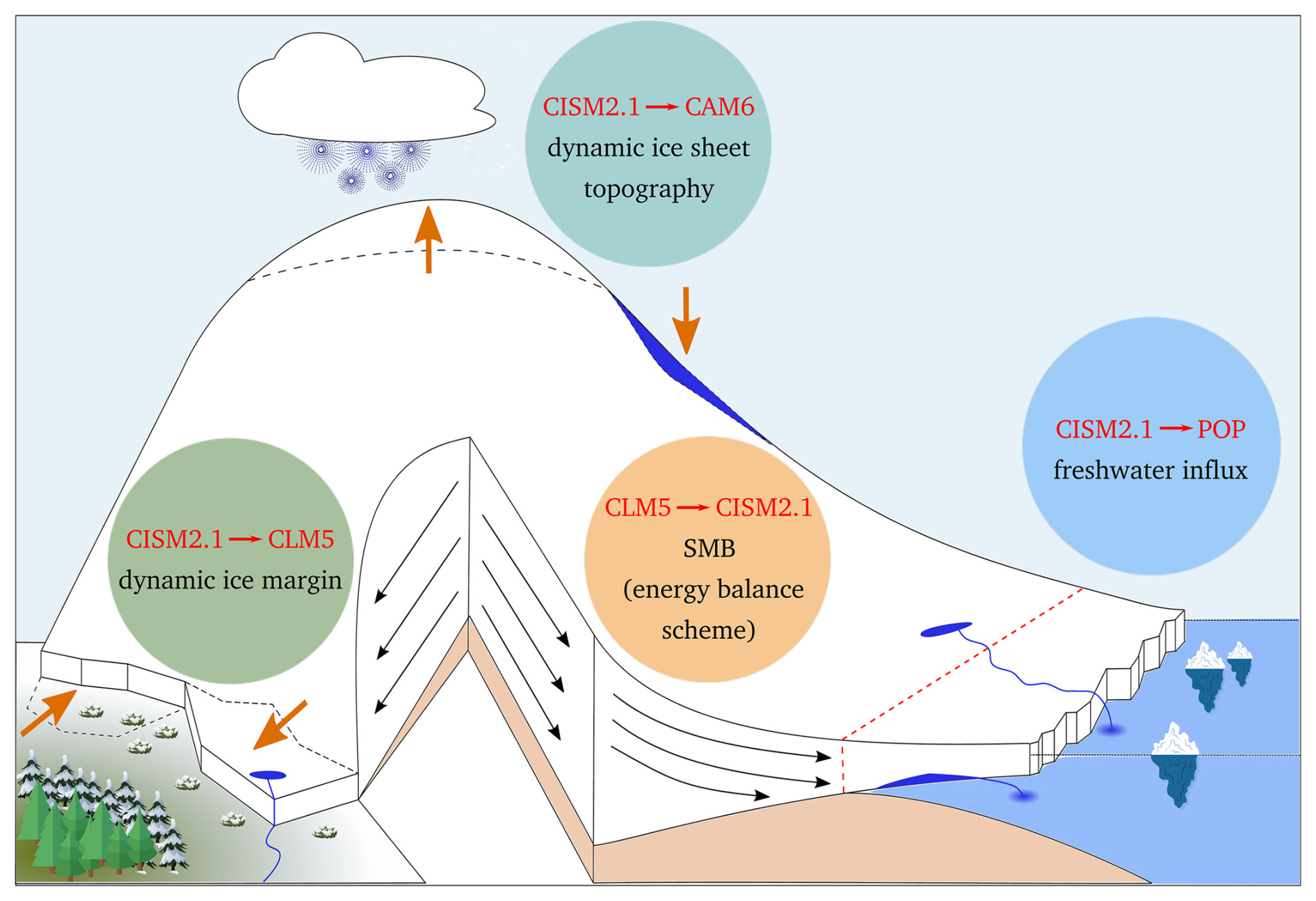
Figure 1 Schematic of four elements of coupling between ice sheets and other Earth system components, courtesy of Michele Petrini (Muntjewerf et al., 2021). The land model (CLM5) receives the location of the ice sheet margin from the ice sheet model (CISM2). The land and the atmosphere (CAM6) models receive the dynamic GrIS topography from the ice sheet model. The ice sheet model provides the freshwater influx from ice discharge to the ocean model (POP), while the land model provides the freshwater fluxes from surface runoff. The ice sheet model itself receives the SMB from the land model to compute changes in the GrIS topography and extent.

The model computes the energy available for melt using the surface energy balance (SEB):

$$\begin{array}{}\text{(2)}& \begin{array}{rl}\text{melt}& =\text{net shortwave}+\text{net longwave}\\ & +\text{latent heat}+\text{sensible heat}\\ & +\text{ground heat}.\end{array}\end{array}$$

The SMB and SEB are computed for multiple elevation classes (Sellevold et al., 2019), which allows for resolving the large heterogeneity around the steep ice sheet margins and for the remapping of the SMB on the ice sheet model grid, which is done using trilinear interpolation and renormalization (Muntjewerf et al., 2021). For every elevation class, the grid cell temperature is downscaled using a uniform lapse rate of −6 K km⁻¹. Precipitation falls as snow if the elevation-corrected near-surface temperature is below −2 °C and as rain if this temperature is above 0 °C. Between −2 and 0 °C, precipitation falls as a mix of rain and snow (Muntjewerf et al., 2021). Based on the downscaled temperature, precipitation and surface energy fluxes, the SMB is computed for every elevation class. Then, the SMB for a grid cell in the land model is the area-weighted average of these elevation classes. Finally, in the ice sheet model, the total GrIS mass balance (MB) is computed as the sum of the SMB downscaled from the elevation classes, basal mass balance and ice discharge. As the ice sheet loses or gains mass, the updated topography and ice sheet margins are communicated to the land model. Here, the land units and topographic height are updated according to the updated ice sheet margins and topography, redistributing the weights of the different elevation classes (Muntjewerf et al., 2021). The changing ice sheet topography influences not only the computations in the land model but also those in the atmosphere component as the topography influences atmospheric circulation. Therefore, the ice sheet topography computed in the ice sheet model is communicated to the atmosphere model, where it is remapped to the atmospheric grid in the form of surface geopotential height (Muntjewerf et al., 2021). Regarding the uni-directional coupling with the ocean, the ice sheet model computes the annual ice discharge and basal melting, which is communicated to the ocean model and then supplied to the ocean at a constant rate throughout the following year. Coupling from the ocean to the ice sheet model is not yet implemented. Therefore, ocean-forced melting of marine-terminating glaciers is not accounted for (Muntjewerf et al., 2021), which could lead to biases in the computed ice discharge. Runoff as a result of melt and rain, computed in the land model, is distributed to the ocean using the river transport model and is therefore seasonally variable.

In this study, we compare with a one-way coupled simulation to quantify elevation feedbacks. The one-way coupled simulation is a simulation in which changes in ice sheet elevation and extent are not communicated to the other model components. The GrIS topography is constant in the land and the atmosphere model, and the freshwater fluxes from the GrIS into the ocean model are fixed. The topography and freshwater fluxes in the one-way configuration are the same as the initial state of the two-way coupled simulation after the spin-up procedure (Lofverstrom et al., 2020). The resulting climate and SMB are downscaled from the fixed land and atmosphere model topography using elevation classes (Sellevold et al., 2019), with a temperature lapse rate of −6 K km⁻¹, and are interpolated onto the ice sheet model grid. The coupler communicates the downscaled SMB to the ice sheet model, where a new ice sheet topography is computed. However, this is not communicated to the other model components when using one-way coupling. This implies that in the one-way setup, the downscaling procedure is used to account for both spatial heterogeneity within a grid cell and elevation differences between the ice sheet model and land and atmosphere models caused by ice sheet mass loss. Since the surface albedo is computed in the land model and the land model allows for the albedo to change, the surface albedo is updated in both the one-way and two-way coupled simulation. Therefore, when snow and ice melt or snow accumulates, the albedo is updated.

2.3 Simulation design

We compare a one-way and a two-way coupled simulation, which are both forced with a 4×CO₂ scenario (Fig. 2a). In this scenario, we apply a yearly 1 % increase in CO₂ concentration until 4 times the PI CO₂ concentration (1140 ppm) is reached in year 140. After year 140, we keep the CO₂ concentration constant at 4×CO₂ until year 500. The 4×CO₂ scenario is an extreme warming scenario and, after the year 140, has a similar radiative forcing to that of the SSP5-85 scenario at the end of the 21st century (Muntjewerf et al., 2020a). The one-way coupled simulation is an extension of the simulation done by Muntjewerf et al. (2020b). Next, we analyze another simulation branched from our two-way coupled simulation, in which we decrease the CO₂ concentration by an annual 5 % between years 350 and 377 until PI CO₂ conditions are reached, after which the CO₂ concentration remains constant until year 925 (Fig. 9a). The climate and ice sheet exchange information every year for the first 500 years of the simulation. After year 500, the climate does not change rapidly anymore. Therefore, to save computational resources, the coupling is done every 5 years after the year 500. Next to the CO₂ forcing experiments, we use a 300-year two-way coupled PI control simulation (Danabasoglu, 2019) with a constant PI CO₂ concentration for comparison.

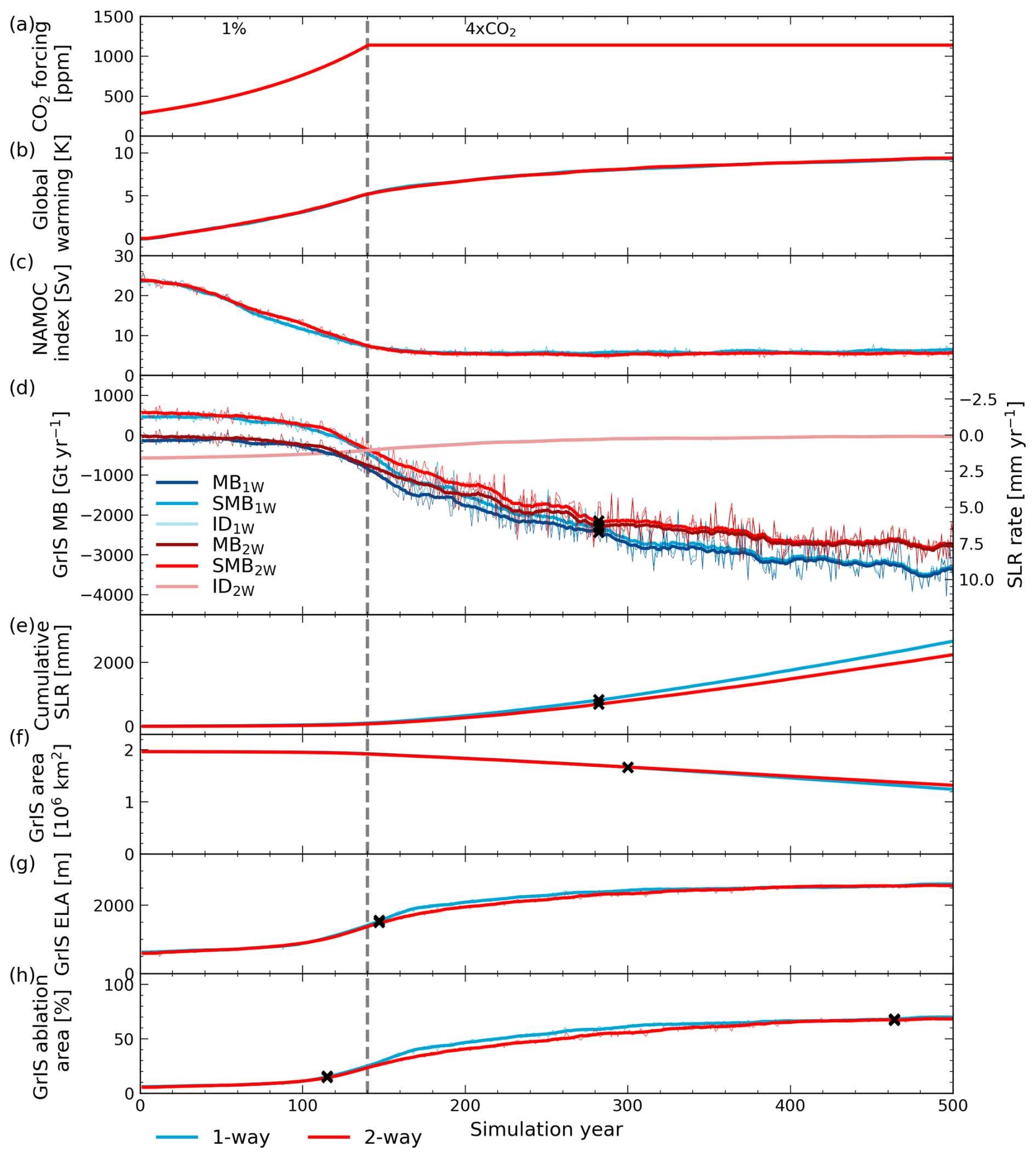
Figure 2 Comparison of forcing, climate and ice sheet evolution of one-way (blue) and two-way (red) coupled simulations for (a) CO₂ forcing [ppm], (b) global warming [K], (c) NAMOC index [Sv], (d) GrIS total mass balance (MB) [Gt yr⁻¹] and its components ice discharge (ID) and surface mass balance (SMB) (the basal mass balance is not displayed as its contribution is limited), (e) GrIS-induced cumulative sea level rise [mm], (f) GrIS area [10⁶ km²], (g) GrIS equilibrium line altitude [m] and (h) GrIS ablation area compared to total GrIS area [%]. The mass balance (components) in (d) can be directly converted to the GrIS-induced SLR rate [mm yr⁻¹]. The dashed grey line indicates the end of the 1 % CO₂ ramp-up period and the start of the continuous 4×CO₂ period. If the differences between the one- and two-way coupled simulations become significant throughout the simulation, the first year of significant difference is marked with a black cross. In (e) the year of significance for the annual SLR is given. In (g) and (h) the year of significant difference before the convergence between the two simulations is given as well.

We consider 20 data points in time for centered moving averages and periodic means to obtain a climatological mean state and variability. This means that before the year 500, 20 years are considered, whereas after the year 500, 100 years are considered. As the climate evolves less rapidly after the year 500, a 100-year mean will be able to represent the mean state of the climate while being consistent in terms of variability compared to the period before the year 500.

2.4 Emergence and recovery

We use the emergence concept applied by Fyke et al. (2014) to assess whether the differences between the one- and two-way simulations are significant. We define the first year of significant difference as the first year when the 20-year centered moving average of the differences between the one- and two-way simulation emerged from the natural variability of the differences. We define the natural variability of the differences as all absolute values smaller than 1 standard deviation of the differences (1σ_differences). To obtain σ_differences, we use the standard deviations computed from the two-way coupled PI control simulation (σ_control). We assume that this control simulation can represent the mean state of a similar one-way control simulation as the ice sheet is nearly in equilibrium, with a limited mean SLR rate of 0.03 mm yr⁻¹, and its variance only represents natural variability. Then, using error propagation, we can express the 1σ_differences interval in terms of σ_control as $[-{\mathit{\sigma }}_{\text{control}}\sqrt{\mathrm{2}}$, ${\mathit{\sigma }}_{\text{control}}\sqrt{\mathrm{2}}]$. When the 20-year centered moving average of the difference has migrated permanently outside the 1σ interval, we consider the signal emerged.

To assess whether climate and ice sheet variables can recover to their PI state after the reintroduction of PI CO₂ levels, we apply a modified approach of the aforementioned emergence concept. A variable is considered recovered if the 20-year centered moving average returns within 1 standard deviation (1σ) of the PI mean and stays within the 1σ interval (obtained from the PI control simulation) for the remainder of the simulation. In case a variable has not recovered by the end of the simulation, we compute an extrapolated year of recovery from the remaining linear trend over the last 100 years (825–925) and the remaining anomaly of the mean state of the variable in the last 100 years of the simulation with respect to the closest boundary of the 1σ confidence interval. We compute the relative amount of recovery by comparing the remaining anomaly in the final 100 years of the simulation to the maximum response during the 4×CO₂ forcing period.

3 Simulated mass loss in the one- and two-way coupled simulation

To assess the impact of simulating an interactive ice sheet, we first consider differences in the global and regional climate to see whether this affects or is affected by GrIS mass loss. As a response to the CO₂ forcing (Fig. 2a), global temperatures rise, with a global warming response of nearly 10 K by year 500, which is not affected by the coupling (Fig. 2b). Under the 4×CO₂ forcing, the North Atlantic Meridional Overturning Circulation (NAMOC; the maximum strength of the overturning stream function north of 28° N and below 500 m depth) collapses in around 150 years in both simulations (Fig. 2c). A near-zero GrIS integrated mass balance in the first 120 years (Fig. 2d) results in limited mass loss in this period (Fig. 2e). During these years, the NAMOC evolution in the one- and two-way coupled simulations is similar, showing that this NAMOC collapse is not strongly related to increased freshwater fluxes from the GrIS.

After year 120, there is an accelerating decrease in SMB, which is the strongest in the one-way coupled simulation (Figs. 2d and A1g–j), leading to the separation of the SLR curves at the year 282 (Fig. 2e). In contrast, the contribution from ice discharge decreases in both simulations due to the melt–discharge feedback as the ice sheet starts retreating (Fig. A1b–e). Because of the small ice discharge contribution in both simulations, the total mass balance differences emerge in the same year as the SMB. After emergence, the one-way coupled simulation consistently projects 17.0±0.4 % more mass loss (p<0.01). GrIS area loss acceleration is slightly delayed compared to the mass loss, and the differences become significant in year 300 (Fig. 2f). Ice mass is mainly lost at the margins, although less strongly in the two-way coupled simulation (Fig. A1b–e). The increased melting of the ice sheet is reflected in the rise in the equilibrium line altitude (ELA; Fig. 2g) and the expansion of the ablation area (the area with negative SMB; Fig. 2h). As melting is stronger in the one-way case, the ablation area expands faster and the ELA heightens faster. However, the ELA and percentage of the ice sheet that experiences ablation in the two simulations converge in years 320 and 400, respectively. As the GrIS loses mass, the equilibrium line moves more inland, but its altitude does not increase strongly anymore as the ice sheet's elevation decreases simultaneously. As the ice sheet extent becomes smaller, parts of the ablation area are lost, slowing down the increase in the total percentage of the ablation area. The period of this slow increase is reached later in the two-way simulation but results in a period (years 400–464) during which ablation and accumulation areas are similar in both simulations.

4 Climate feedback response to a dynamic GrIS topography

The differences in the mass balance evolutions of the two simulations indicate that the local climate and GrIS surface processes are affected by the coupling. We first consider the positive melt–elevation feedback, which enhances mass loss, and assess its representation in the one-way coupled configuration as we compute the climate using a fixed topography in the one-way simulation. Then, we analyze feedbacks related to atmospheric processes by considering atmospheric circulation, clouds and precipitation.

4.1 The melt-elevation feedback

The melt response to the CO₂ forcing causes a lowering of the topography (Fig. A1a–e). This triggers the melt–elevation feedback (Fig. 3), as lower elevations coincide with higher temperatures, and consequently enhances the melt–albedo feedback, as bare ice and melting snow have a lower albedo. In the two-way simulation, we account for this by allowing the topography to evolve in the land model, while in the one-way simulation, the topography is constant. The effect of incorporating a dynamic topography on the melt becomes significant in year 215, and accounting for this leads to 66 % more melt in the land model in the two-way simulation compared to the one-way simulation by year 500. Since both simulations include an interactive calculation of the albedo, the melt differences include both the melt–elevation and the resulting enhancement of the melt–albedo feedback. A quantification of the strength of this feedback has been done by Muntjewerf et al. (2020b). Next to the albedo, the melt is affected by atmospheric-related feedbacks as well.

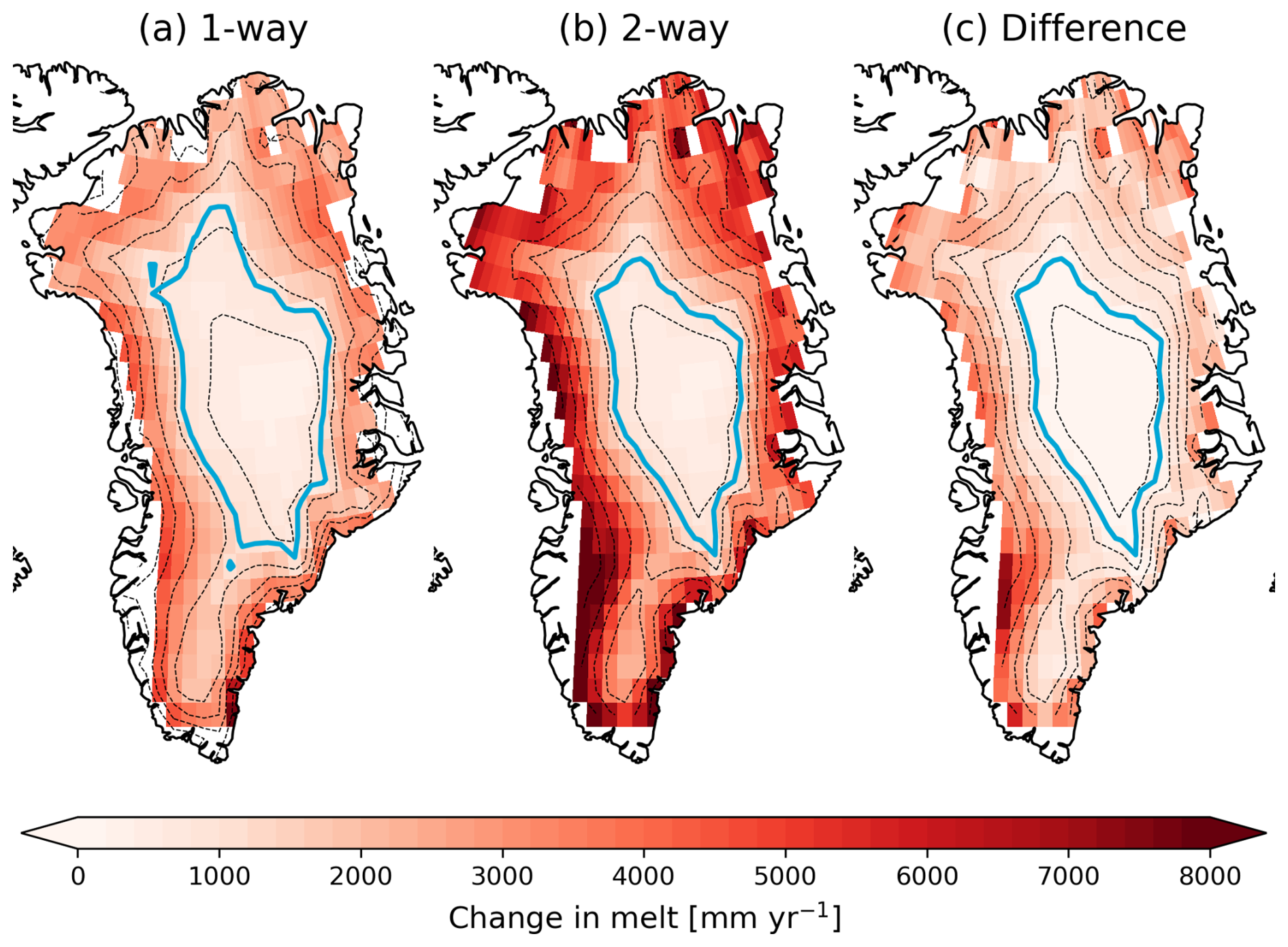
Figure 3 Change in melt [mm yr⁻¹] as modeled by the land model (CLM5) for years 480–500 with respect to the control simulation over the ice sheet extent of the two-way simulation for the (a) one-way and (b) two-way coupled simulation. (c) difference between (a) and (b), showing the effect of topographic change on melt evolution. The dashed black lines depict contour lines for every 500 m elevation of (a) the one-way and (b–c) the two-way simulation. The light blue line represents the ELA of (a) the one-way and (b–c) the two-way simulation. All changes are significant according to the emergence criterion (Sect. 2.4).

The 2 m air temperature (T_2 m) increase as a response to elevation changes causes changes in the GrIS surface energy fluxes. The downscaling of the T_2 m and the downwelling longwave radiation (LW_in) has a large influence on the computed SEB (Sellevold et al., 2019). To assess the effect of the elevation change on these variables, we compute lapse rates resulting from elevation changes (Fig. 4 – monthly means, Fig. A2 – seasonal maps) and compare them with the applied lapse rates for elevation change in the one-way coupled simulation (Table 1). These lapse rates are computed by dividing the difference in the mean state of a variable between the one- and two-way simulation by the difference in elevation between the one- and two-way simulation for the years 480–500. Thresholds of 250 m elevation difference and an ice sheet fraction of 90 % of the grid cell are taken to exclude grid cells in which most of the changes are not caused by elevation changes. It should be noted that these lapse rates describe the change in a variable caused by GrIS surface changes rather than the rate of change over a changing pressure level as described by the free-atmospheric lapse rate.

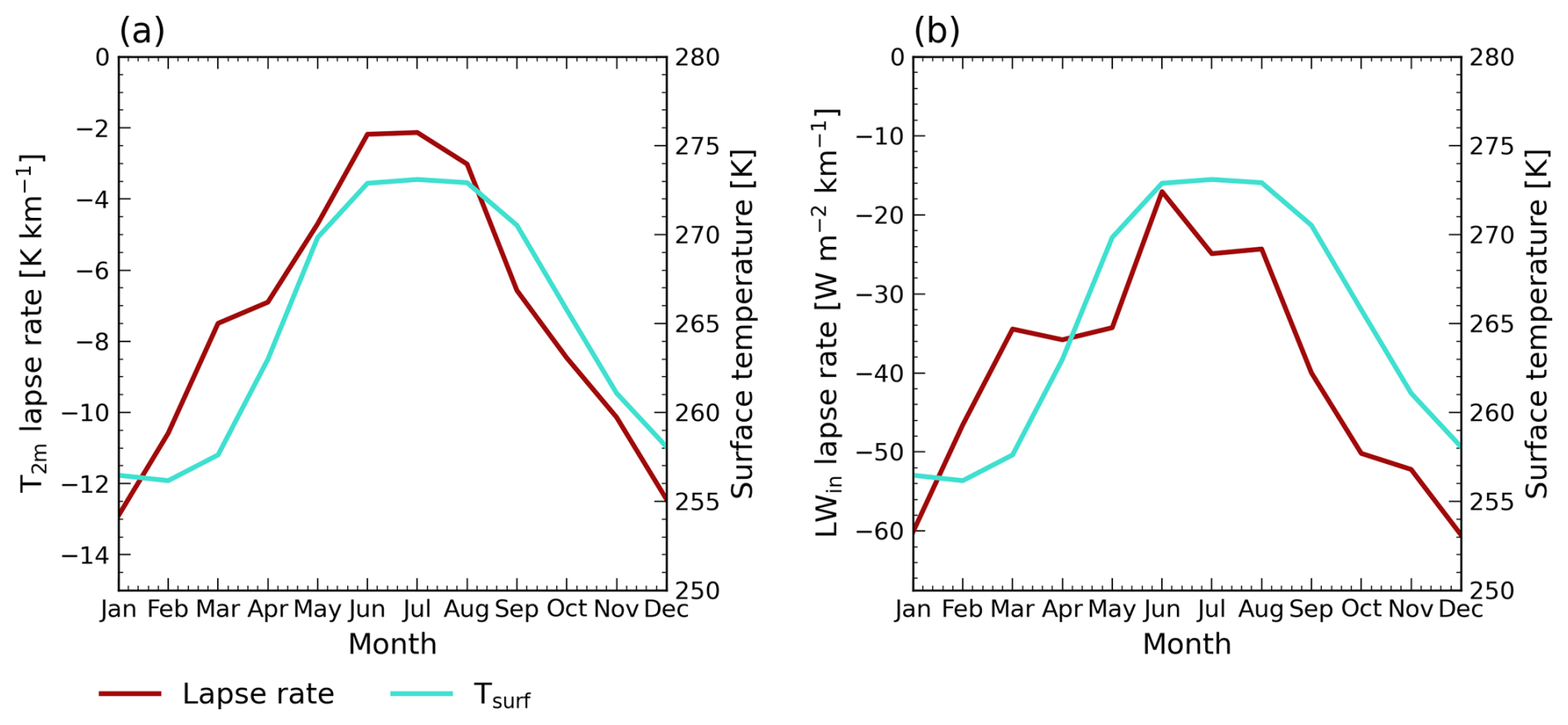
Figure 4 Monthly mean lapse rates (dark red) for (a) 2 m air temperature [K km⁻¹] and (b) incoming longwave radiation [$\mathrm{W}{\mathrm{m}}^{-\mathrm{2}}{\mathrm{km}}^{-\mathrm{1}}$] for years 480–500. The light blue line shows the monthly mean surface temperature [K] of the locations considered for computing the lapse rates and is the same in both (a) and (b). The locations considered for the mean lapse rates and surface temperatures are shown in Fig. A2.

Table 1 2 m air temperature [K km⁻¹] and downwelling longwave radiation [$\mathrm{W}{\mathrm{m}}^{-\mathrm{2}}{\mathrm{km}}^{-\mathrm{1}}$] lapse rates for annual, summer (June, July, August) and winter (December, January, February) means, compared to the applied lapse rates in the one-way coupled simulation, computed using the years 480–500. The number within brackets represents 1 standard deviation in the spatial domain.

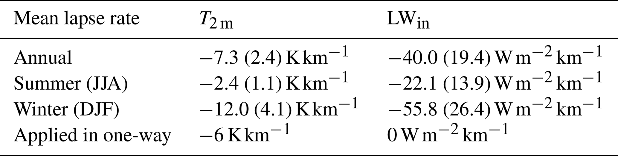
The one-way lapse rate of −6 K km⁻¹ corresponds relatively well to the annual mean temperature lapse rate (Table 1). However, applying these pre-defined lapse rates leads to an overestimation of the T_2 m in summer and an underestimation in winter. The overestimation in summer is partly compensated by not applying an LW_in lapse rate, resulting in an underestimation of LW_in in the one-way coupled simulation. In summer, the surface in the ablation area, which is the area in which most of the elevation change happens, is at the melting point (Fig. 4). Therefore, part of the available energy will be used for melting instead of heating the atmosphere, leading to a limited T_2 m increase in the ablation area. The LW_in lapse rates show a similar pattern as these are largely influenced by atmospheric temperatures.

To assess the effect of the difference in applied lapse rates, we consider a point that transitions from the accumulation to the ablation area (66.44° N, 45° E, shown in Fig. A2). Here, the one- and two-way simulations show a similar response as long as the elevation does not change (Fig. 5). As soon as the mean summer surface temperature reaches the melting point (Fig. 5c, dashed orange line) and elevation starts to lower (Fig. 5a), T_2 m and melt responses start to diverge between the simulations. Since in the one-way simulation the temperature and surface fluxes correspond to a fixed elevation, melt does not increase as strongly as in the two-way case. However, adding the temperature change due to the lowering of the elevation by considering the −6 K km⁻¹ lapse rate (dashed blue line in Fig. 5c) results in a large overestimation of the one-way T_2 m, potentially causing an overestimation of the sensible and latent heat flux contribution to the melt energy. Although this is partially compensated by an underestimation of the incoming longwave flux, this could lead to an overestimation of the melt–elevation and melt–albedo feedback when computing mass loss in the ice sheet model, which could explain part of the overestimated mass loss.

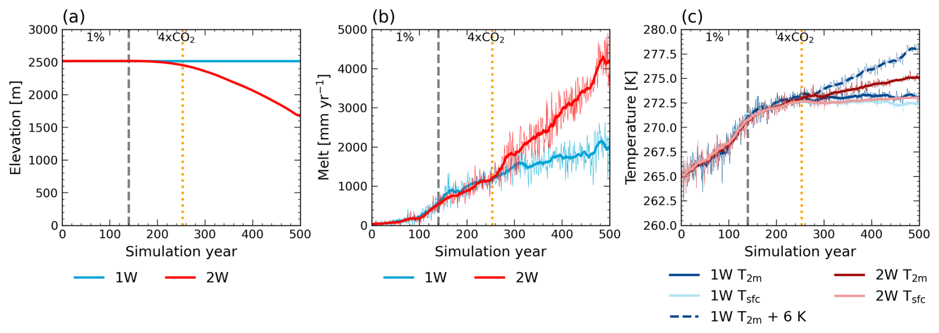
Figure 5 Evolution of (a) elevation [m], (b) annual melt [mm yr⁻¹] and (c) mean summer (June, July, August) 2 m air and surface temperature [K] for the one-way (blue, 1 W) and two-way (red, 2 W) coupled simulations for a point that transitions to the ablation area (66.44° N, 45° E, shown in Fig. A2). The dashed grey line indicates the end of the 1 % CO₂ ramp-up period and the start of the continuous 4×CO₂ period. The dashed orange line indicates the timing of reaching surface melt conditions throughout the whole summer (273 K). In (c) the dashed blue line shows the evolution of one-way T_2 m when applying the −6 K km⁻¹ lapse rate to the two-way elevation change.

4.2 Elevation feedbacks related to changes in precipitation, atmospheric circulation and clouds

Besides affecting temperature, changes in the GrIS topography can change the local climate in several other ways. First of all, the effect of the presence of the cold and high-elevation GrIS on atmospheric circulation might change as its surface lowers and warms, which might have large implications for the regional climate. Atmospheric blocking events, associated with persistent high-pressure conditions over Greenland, can be related to higher summer temperatures and reduced cloud cover over Greenland (Hofer et al., 2017). Therefore, increases in the amount of summer atmospheric blocking have been linked to increased melt (Hanna et al., 2014, 2022; McLeod and Mote, 2015). We compute the Greenland blocking index (GBI) using the method proposed by Hanna et al. (2018) (GB2) for both the summer (JJA) and winter (DJF). We subtract the area-weighted mean of the 500 hPa geopotential height over the Arctic region (60–80° N) from the Greenland region (60–80° N, 20–80° W) and normalize using the variability of the control simulation. We find a large reduction in the Greenland blocking index resulting from a changing GrIS surface (Fig. 6a and b), especially in summer. This aligns with the positive relationship between orography and blocking events (Mullen, 1989; Narinesingh et al., 2020; Sellevold et al., 2022). As the large changes in GrIS topography might have large influences on the atmospheric circulation around Greenland as a whole, our computed changes in the blocking index may not only consist of changes in blocking but are influenced by other changes in atmospheric circulation as well. Additionally, we find that the changing GrIS geometry has no significant effect on the phase of the North Atlantic Oscillation (NAO; the principle component corresponding to the leading empirical orthogonal function of the seasonal sea level pressure in the North Atlantic region (20–80° N, 90° W–40° E) normalized using the variability of the control simulation; Hurrell, 1995) (Fig. 6d and e). However, the summer NAO index shows a trend towards a positive phase as a response to the warming in both simulations (p<0.001).

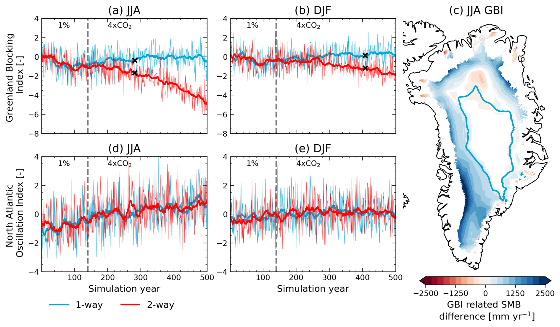
Figure 6 Evolution of (a, b) Greenland blocking index (GBI) [–] and (d, e) North Atlantic Oscillation (NAO) index [–] for (a, d) June–July–August (JJA) mean and (b, e) December–January–February (DJF) mean for the one-way (blue) and two-way (red) coupled simulations. The dashed grey line indicates the end of the 1 % CO₂ ramp-up period and the start of the continuous 4×CO₂ period. If the differences between the one- and two-way coupled simulations become significant throughout the simulation, the first year of significant difference is marked with a black cross. (c) shows the difference in SMB [mm yr⁻¹] caused by the coupling that can be explained by the difference in summer blocking index, computed using linear regression for the area with significant Pearson correlation (p = 0.01) for the years 480–500, for grid points that have not deglaciated in both simulations. The light blue line represents the ELA in the two-way simulation in years 480–500.

To relate the decrease in blocking index to the projected mass loss, we regress the GBI differences between the one- and two-way coupled simulations onto the SMB differences (from CISM2; Fig. 6c). A positive regression coefficient indicates a linear relationship between the differences in the blocking index and the differences in SMB reduction, and its magnitude represents the slope of this linear relationship. The relationship between the GBI and SMB differences is the strongest in the ablation area. In the accumulation area, the surface melt is limited, which is likely the reason why we do not find a strong relationship with changes in GBI. As the topographies of the two simulations evolve differently, so does the SMB pattern, resulting in small areas in which the correlation signal is negative, indicating a slightly larger SMB reduction in the two-way coupled simulation. This might not be caused by the differences in blocking index but rather by differences in the topography. Considering areas with significantly strong correlation (positive or negative, as tested with a t test using p = 0.01), we can link 49 % of the difference in SMB reduction between the two simulations at the final simulation years to the decrease in GBI (Fig. 6c). As the SMB differences are mainly dominated by melt differences in this period, we hypothesize that the decrease in blocking as a result of GrIS surface elevation changes (Fig. A1a–e) acts as a negative feedback on surface melting.

We find another negative feedback, this time related to clouds and water vapor. Under increasing temperatures, the atmosphere can contain more moisture (as described by the Clausius–Clapeyron relationship), which can lead to an increase in clouds and enhanced precipitation (Pall et al., 2007). The amount of precipitable water in the atmospheric column (Fig. 7d) increases in both simulations, although more strongly in the two-way coupled simulation, as the atmospheric column warms more and becomes larger as a result of elevation change. The increase in precipitable water translates to a stronger reflection and absorption of incoming solar radiation in the atmosphere (Fig. 7a). The differences in the atmospheric effect on incoming shortwave radiation and precipitable water both become significant in year 262, indicating they are strongly related. There is no increase in cloud cover (Fig. 7b) in either of the simulations or even a slight decrease in medium-level clouds. However, cloud cover itself does not strongly control the incoming shortwave radiation. Instead, the cloud optical thickness, influenced by the presence of liquid water and ice in the atmosphere, is an important determining factor for the incoming shortwave radiation (Ettema et al., 2010). As the cloud water path (Fig. 7c) increases throughout the simulation, meaning clouds become thicker, more shortwave radiation is reflected. This effect is stronger than the effect caused by the slight decrease in cloud cover, resulting in a stronger cloud effect on incoming surface solar radiation (Fig. 7a) in the two-way coupled simulation. The differences in cloud water path and cloud effect on downwelling shortwave radiation both become significant in year 401, showing that the cloud thickness is the determining factor for incoming shortwave radiation rather than cloud cover.

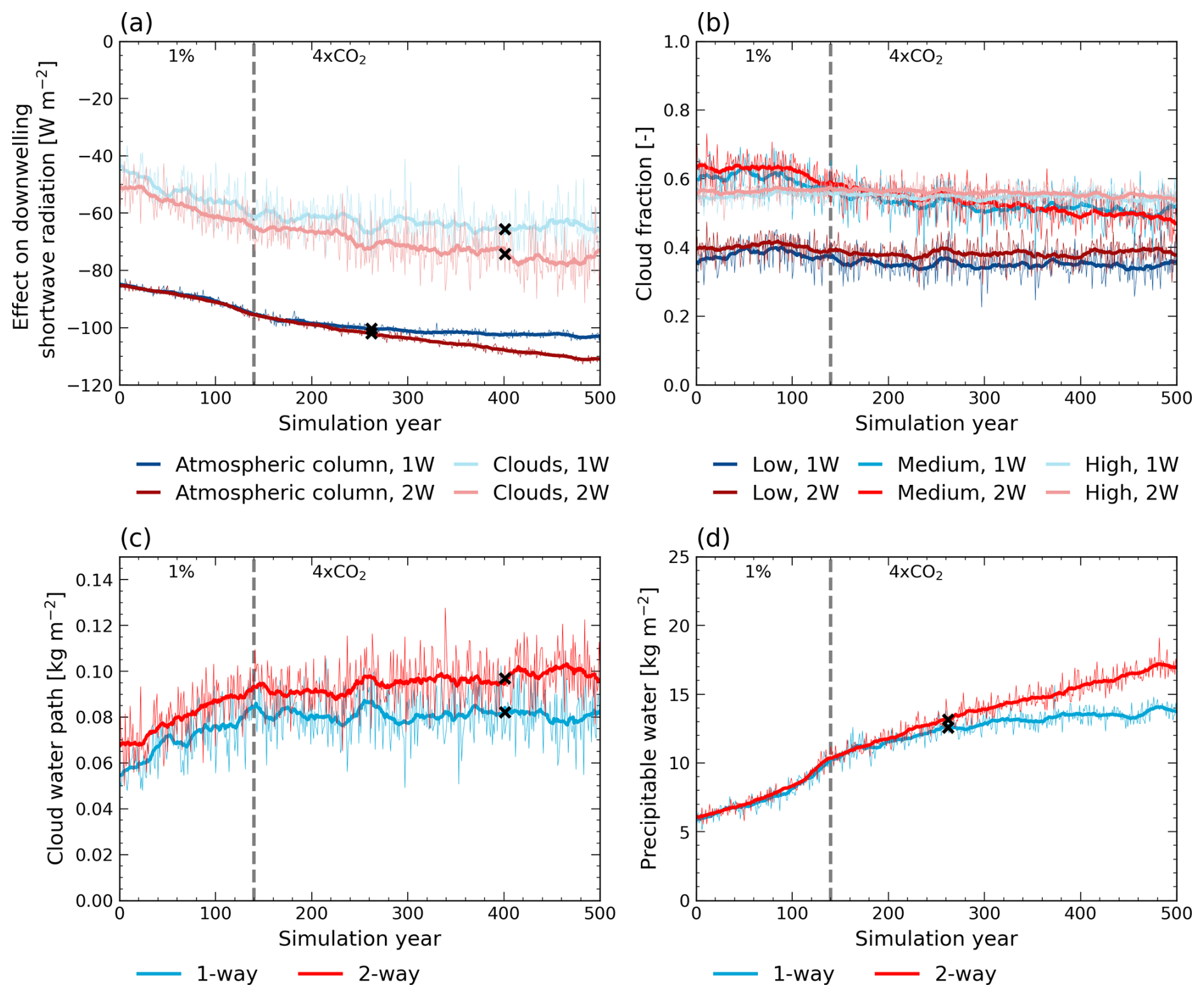
Figure 7 Time series over the first-year ice sheet extent of one-way (blue, 1 W) and two-way (red, 2 W) simulations for (a) effect on downwelling shortwave radiation [W m⁻²] of the atmospheric column and clouds. The effect of the atmospheric column is computed by comparing the incoming solar radiation at the top of the atmosphere with the received radiation at the surface for cloud-free conditions. The effect of clouds is computed by comparing the incoming solar radiation at the top of the atmosphere with the received radiation at the surface for all-sky conditions and correcting for the effect of the atmospheric column. (b) cloud fraction [–] for low-, medium- and high-level clouds, (c) cloud water path [kg m⁻²] and (d) precipitable water in the atmospheric column [kg m⁻²]. The dashed grey line indicates the end of the 1 % CO₂ ramp-up period and the start of the continuous 4×CO₂ period. If the differences between the one- and two-way coupled simulations become significant throughout the simulation, the first year of significant difference is marked with a black cross.

Finally, a lowering topography leads to an overall increase in precipitation, especially in the southeast (Fig. 8a). Higher temperatures in the two-way simulation result in more evaporation from the surrounding oceans. An increase in the transport of this moisture leads to increased precipitation over the GrIS (Fig. 8d). In some locations in the western and northern margins, precipitation decreases, although not significantly in all locations, as orographic precipitation moves more land inward, following the margin. In the western margins, we see a corresponding strong increase in integrated vapor transport (IVT; specific humidity times the wind velocity, integrated from 1000 to 300 hPa and normalized by the gravity; Reynolds et al., 2022). The difference in precipitation is mainly caused by increased rainfall (Fig. 8c) rather than increased snowfall (Fig. 8b). Snowfall moves more towards the interior as temperatures in the margins become too high for precipitation to fall as snow. As a result, snowfall decreases in the ablation area and increases in the accumulation area (Fig. A3). The increase in snowfall in the interior contributes positively to the SMB, acting as a negative feedback. However, the elevation effect on temperature results in a larger fraction of rainfall, which can enhance the melt–albedo feedback. Therefore, the changes in rainfall can be considered a positive feedback.

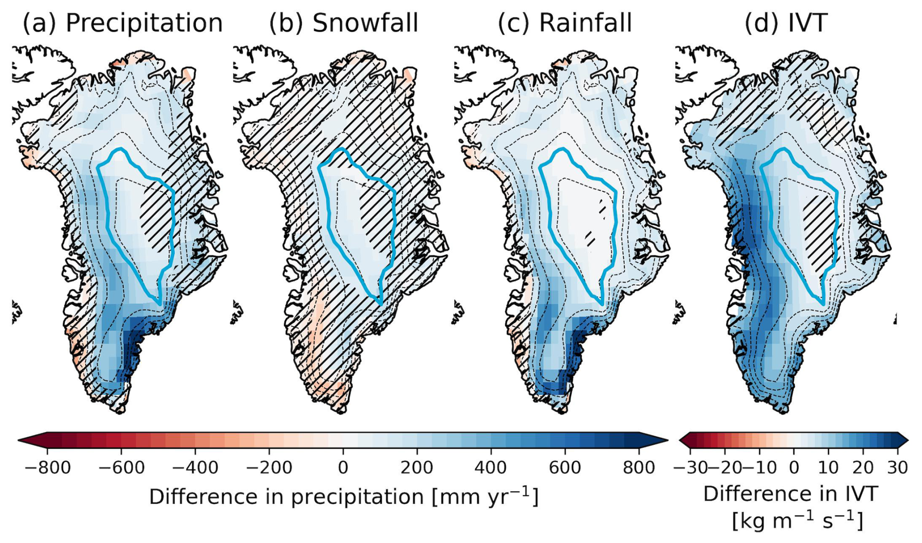
Figure 8 Annual mean differences (two-way minus one-way) resulting from the coupling for (a) total precipitation [mm yr⁻¹] (the sum of snowfall and rainfall) (b) snowfall [mm yr⁻¹], (c) rainfall [mm yr⁻¹] and (d) mean integrated vapor transport (IVT) [$\mathrm{kg}{\mathrm{m}}^{-\mathrm{1}}{\mathrm{s}}^{-\mathrm{1}}$] for years 480–500 over the first-year ice sheet extent. The dashed black lines depict contour lines for every 500 m elevation of the two-way simulation. The light blue line represents the ELA of the two-way simulation. Hatches denote areas in which the differences between the one- and two-way coupled simulations have not become significant before the year 500.

5 Ice sheet–climate interactions and mass balance response under reintroduction of PI CO₂ conditions

The 4×CO₂ forcing triggers large responses in global, Arctic and GrIS temperatures (Figs. 2b and 9b). By year 350, the GrIS has a strongly negative mass balance in the two-way coupled simulation (Figs. 2d and 9d), causing an SLR rate of 6.6±1.0 mm yr⁻¹, with a cumulative GrIS SLR contribution of 1.13 m (Figs. 2e and 9e). The discharge contribution to the mass balance is limited ($-\mathrm{78}\pm \mathrm{8.8}$ Gt yr⁻¹) as the ice sheet has strongly retreated. Besides, the NAMOC has collapsed (Figs. 2c and 9c), reducing the amount of northward heat transport. We branch another simulation from the two-way coupled simulation, starting in year 350, and apply an annual 5 % CO₂ reduction until PI CO₂ conditions are reached in year 377 (Fig. 9a) to assess ice sheet–climate interactions and the resulting mass balance as a response to CO₂ reduction. We first consider global, Arctic and North Atlantic climate change and evaluate the GrIS mass loss response to CO₂ reduction. We zoom in to the first century after the CO₂ reduction, which is characterized by a complex transition phase towards a colder climate, and look at the NAMOC evolution and its impact on regional climate. Finally, we assess GrIS surface processes by considering the response of the snowpack.

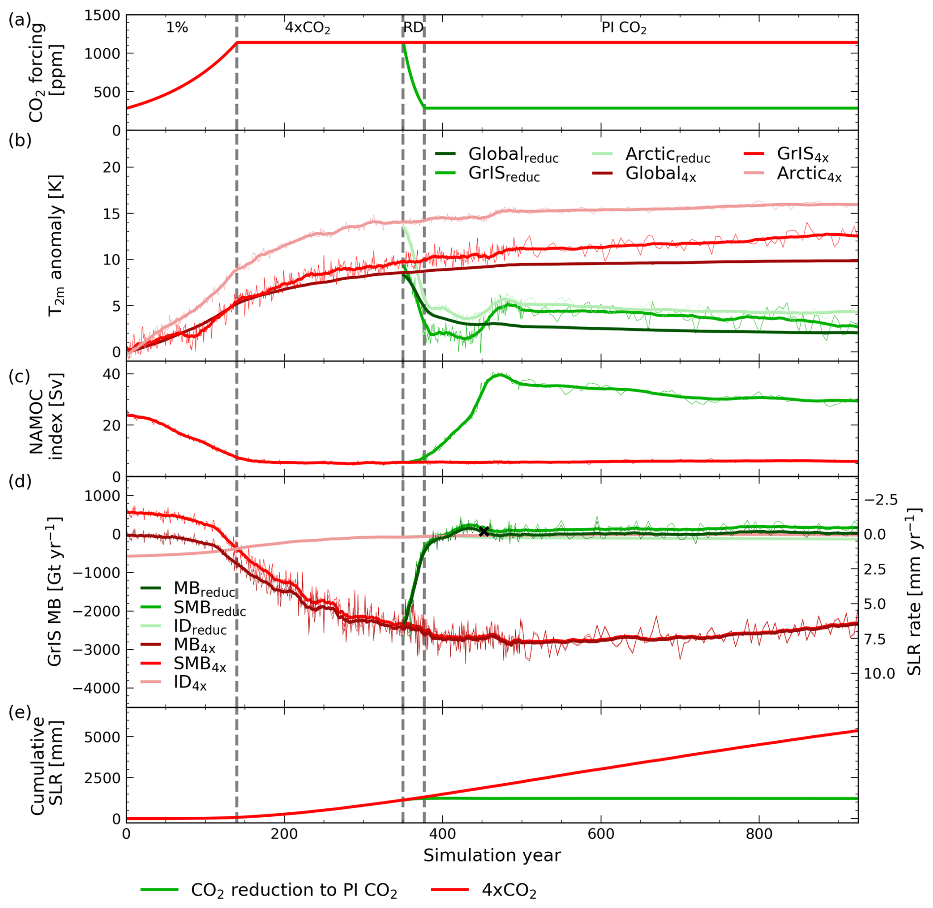
Figure 9 Evolution of CO₂ reduction to pre-industrial CO₂ (green, reduc) and the full 4×CO₂ (red, 4×) simulations for (a) CO₂ forcing [ppm], (b) global, evolving GrIS and Arctic near-surface air temperature (T_2 m) anomalies with respect to PI [K], (c) North Atlantic Meridional Overturning Circulation (NAMOC) index [Sv], (d) GrIS total mass balance (MB) [Gt yr⁻¹] and its components ice discharge (ID) and surface mass balance (SMB) (the basal mass balance is not displayed as its contribution is limited) and (e) GrIS cumulative sea level rise contribution [mm]. The mass balance (components) in (d) can be directly converted to the GrIS-induced SLR rate [mm yr⁻¹]. The dashed grey lines indicate the end of the 1 % CO₂ ramp-up, the continuous 4×CO₂, the ramp-down (RD) to PI CO₂ and the continuous PI CO₂ periods. If a variable has recovered throughout the simulation, the first year of recovery is marked with a black cross.

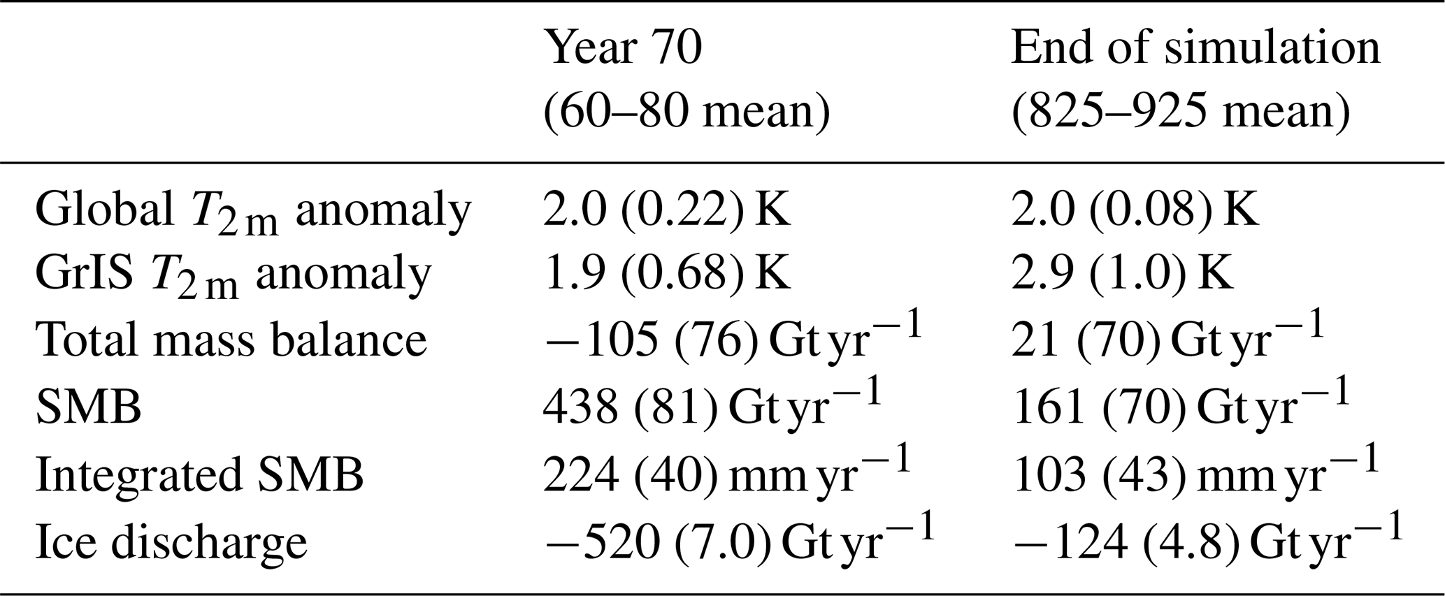
The response to CO₂ reduction can be divided into two periods. During the first period, spanning the 27 years during the CO₂ ramp-down and the following 85 years, the GrIS experiences a complex transitional phase because of strong interactions with the NAMOC. During this phase, the NAMOC is still weak as its recovery is delayed compared to the atmospheric response, giving rise to relatively cold temperatures in the Arctic and over the GrIS (Fig. 9b). Under these largely reduced air temperatures resulting from the CO₂ decrease and weak state of the NAMOC, the amount of GrIS melt decreases strongly, leading to a small positive SMB and MB (Fig. 9d). During the CO₂ ramp-down and first years thereafter, there is an additional SLR of 1.18 m. This is followed by a short period (years 413–461) of positive mass balance, leading to a 0.13 m sea level drop, after which GrIS SLR contribution is halted (Fig. 9d and e). The second period, spanning from the end of the transitional phase (year 462) to the end of the simulation, is characterized by initial temperature increases in the Arctic and over the GrIS as a response to an overshooting rebound of the NAMOC followed by a slow continuous decrease in atmospheric temperature and NAMOC strength. The mass balance becomes smaller than during the transitional phase, nearing zero, and recovers to its PI state (0.04±0.23 mm yr⁻¹) by the year 452 (Table B1). However, from year 735 onward, the mass balance becomes slightly positive again, leading to an annual sea level drop of 0.06±0.19 mm yr⁻¹ at the end of the simulation. This indicates that there might be potential for ice sheet regrowth, although at this rate this would take over 10 000 years. At the end of the simulation, the SMB does not recover (Table B1) as global and GrIS temperatures remain elevated compared to the initial state. However, the coinciding retreated ice sheet margins result in a smaller contribution of ice discharge to the mass balance compared to the first 2 centuries (Fig. 9d). Together with a small positive SMB, the small negative contribution of the ice discharge allows for a small positive total mass balance. We compare this state to the state of the GrIS under the same global T_2 m anomaly (2 K) during the CO₂ ramp-up (year 70), where we see an ice sheet that is largely marine-terminating and is out of balance as a result of this temperature anomaly (Table 2, Fig. B1). Although the ice sheet has a stronger positive SMB in year 70, the large ice discharge leads to net mass loss, while for the retreated ice sheet at the end of the CO₂ reduction simulation, the total mass balance is slightly positive despite the smaller SMB.

Table 2 Comparison of the state of the GrIS under an annual global T_2 m anomaly of 2.0 K during the CO₂ ramp-up period in year 70 (average over years 60–80) and at the end of the CO₂ reduction simulation (average over years 825–925). The number within brackets represents 1 standard deviation. A topographic representation of these states can be found in Fig. B1.

During the 4×CO₂ forcing period, the North Atlantic warms less rapidly due to the weakening of the NAMOC, resulting in a warming hole southeast of Greenland (Fig. 10a). During the transitional CO₂ reduction phase, the North Atlantic cools rapidly as this warming hole persists under a weak NAMOC (Fig. 10c). However, the delayed NAMOC overshoot causes the North Atlantic temperatures to subsequently rise, causing the warming hole to disappear (Fig. 10e). Besides, the timing of changes in GrIS, North Atlantic and Arctic processes strongly coincides with the timing of NAMOC index changes (Fig. B3), highlighting the complexity of the interactions between the ocean, atmosphere, Arctic sea ice and GrIS.

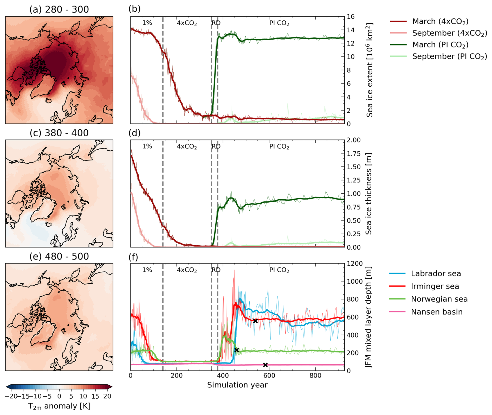
Figure 10 (a, c, e) Mean anomalies of near-surface temperature (T_2 m) [K] for the CO₂ reduction simulation compared to the control simulation for (a) years 280–300 during the constant 4×CO₂ period, (c) years 380–400 just after the CO₂ ramp-down in the transition period and (e) years 480–500 after the transition period. (b, d) Evolution of reduction to pre-industrial CO₂ (green) and the full 4×CO₂ (red) simulations for (b) sea ice extent [10⁶ km²] and (d) sea ice thickness [m] of the evolving sea ice extent in March and September. (f) Evolution of the mean mixed layer depth (MLD) of January, February and March (JFM) in the Labrador Sea (blue), Irminger Sea (red), Norwegian Sea (green) and Nansen Basin (pink) for the reduction to pre-industrial CO₂ simulation. In (b), (d), (f) the dashed grey lines indicate the end of the 1 % CO₂ ramp-up, the continuous 4×CO₂, the ramp-down (RD) to PI CO₂ and the continuous PI CO₂ periods. If a variable has recovered throughout the simulation, the first year of recovery is marked with a black cross.

The Arctic interacts strongly with the NAMOC and the atmosphere. Due to a large drop in Arctic T_2 m as a response to reverting CO₂ conditions, the March Arctic sea ice extent (the area north of 60° N where sea ice concentration is greater than 15 %) recovers quickly (Fig. 10b), amplified by the thin ice feedback (Notz, 2009), as an area with thin sea ice expands faster. In contrast, the September sea ice does not recover since the newly formed sea ice is relatively thin (Fig. 10d), and ocean and atmosphere summer temperatures remain elevated. Besides, the sea ice melt is amplified by the sea ice–albedo feedback (Curry et al., 1995), leading to the nearly complete melting of the recently formed sea ice in summer. The regrowth of sea ice in winter influences the NAMOC strength as brine rejection leads to more saline high-latitude waters, enhancing overturning. The overshooting response of the NAMOC leads to a subsequent decrease in Arctic sea ice extent and thickness as a result of increased northward heat transport.

The mixed layer depth (MLD; Fig. 10f), which is an indicator of the amount of overturning and thus of the strength of the NAMOC, decreases in the Labrador Sea, Irminger Sea and Norwegian Sea during the 1 % CO₂ ramp-up period. In contrast, the MLD in the Nansen Basin starts to increase slightly. This indicates a movement of the area with strong overturning towards higher latitudes, which is possibly caused by the decrease in Arctic sea ice extent (Fig. 10b). The MLDs in the Labrador Sea, Irminger Sea and Norwegian Sea all experience an overshoot after the CO₂ ramp-down, similarly to the NAMOC index. Only in the Labrador Sea, where we see the large remaining temperature anomalies as well (Fig. 10c) – indicating elevated heat transport, is there no complete recovery from the overshoot.

Looking at GrIS surface processes, we find that melt increases due to the CO₂ forcing are partly countered by enhanced refreezing (Fig. 11a). At the end of the ramp-up period, in year 130, the peak in the amount of refreezing is reached despite the ongoing increase in the amount of available water for refreezing. This implies that around this year, the pore space and/or available energy for melt starts to decrease. This peak refreezing behavior is typical of high-emission scenarios (Noël et al., 2022). The refreezing capacity (amount of refreezing divided by the amount of available water) peaks earlier as the snowpack is not able to refreeze a similar fraction of the larger amount of available water since it does not become thicker concurrently (Fig. B4a). After the CO₂ ramp-down, the amount of refreezing slightly peaks again in year 478 as the snowpack partially recovers. However, the poorer state of the snow compared to its state before the 4×CO₂ forcing was applied, characterized by higher snow temperatures and a thinner snowpack (Fig. B4), prevents the snowpack from returning to refreezing rates similar to year 130 despite the similar amount of available water. Besides, the poorer state of the snowpack, combined with a larger amount of available water than in the initial state, results in a refreezing capacity that does not recover (Table B1).

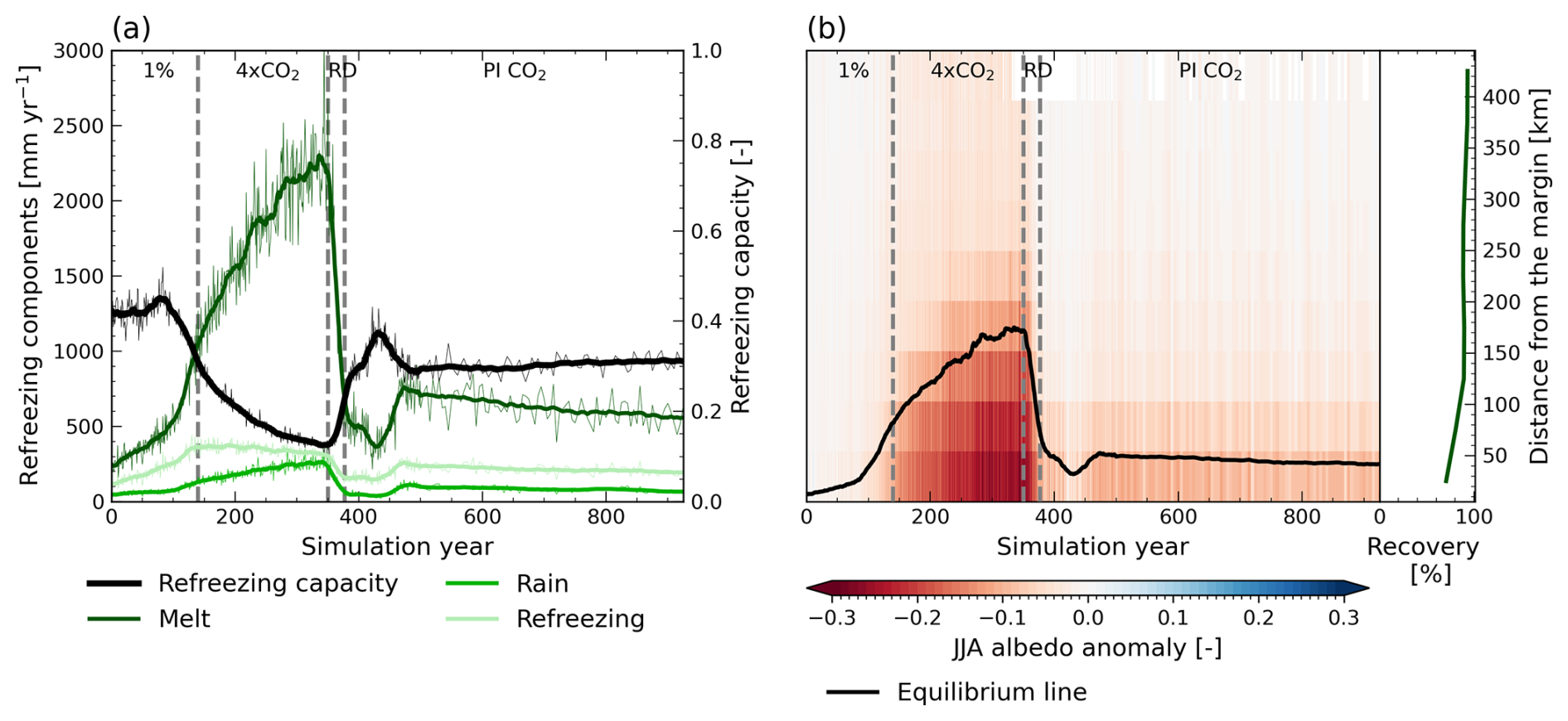
Figure 11 Evolution of the snow properties (a) refreezing capacity (black) [–], defined as the refreezing divided by the amount of available water for refreezing (meltwater and rain) and its components meltwater (dark green), rainfall (green) and refreezing (light green) [mm yr⁻¹] over the evolving ice sheet and (b) summer (JJA) albedo anomalies [–] with respect to the control simulation as a function of time and distance to the ice sheet margin for the reintroduction of PI CO₂ simulation and the location of the equilibrium line (black). In (b), the dark green line shows the relative recovery (in %) for each distance class. The dashed grey lines indicate the end of the 1 % CO₂ ramp-up, the continuous 4×CO₂, the ramp-down (RD) to PI CO₂ and the continuous PI CO₂ periods. None of the variables in (a) have recovered by the end of the simulation.

Next to the refreezing, the ice sheet albedo does not completely recover either (Fig. 11b). In the cooler period around years 400–450, the albedo nearly recovers to its initial state, even around the margins, as melt strongly reduces. However, subsequent temperature increases due to the NAMOC recovery lead to more melt and rain and a corresponding decrease in albedo, aligning with the expansion of the ablation area, resulting in an ELA that does not recover. The lower surface albedo causes the net shortwave flux to remain larger, which is the largest contributor to the fact that the SMB and SEB (Fig. B2) do not recover completely.

6 Discussion

The results presented in this study highlight the importance of accounting for interactions between the GrIS and the climate for SLR projections. We find that uncoupled simulations of ice sheet and climate evolution can lead to an overestimation of the SLR contribution. For CESM2, we find an overestimation of the GrIS SLR contribution of 17 % under a 4×PI CO₂ forcing when using the one-way coupled configuration. Similarly, Ridley et al. (2005) found an overestimation of mass loss in an uncoupled AOGCM-ISM simulation, although these only become apparent after a total mass loss of around 2.5 m sea level equivalent (SLE) as opposed to 0.7 m SLE in our study. Our results are close to those of Gregory et al. (2020), who found a relative overestimation of mass loss of 13 % in an uncoupled abrupt 4×CO₂ simulation using the Glimmer ice sheet model coupled with FAMOUS-ice. Gregory et al. (2020) attributed part of the smaller mass loss in the coupled simulation to a larger precipitation increase as precipitation in the southwest moves land inward, which is similar to what we find. However, the larger amount of rainfall does not contribute positively to the SMB, and, although the snowfall in the accumulation area is larger in the two-way coupled simulation, its contribution is limited (28 Gt yr⁻¹ by year 500, Fig. A3), compared to other feedbacks. Besides, Gregory et al. (2020) related the smaller mass to a negative cloud feedback on the downwelling shortwave radiation due to a larger cloud fraction in the coupled simulation. Although we do not find significant differences in cloud fraction, we find significantly thicker clouds in the two-way coupled simulation. Ettema et al. (2010) indicated that cloud thickness, rather than cloud cover, is the most important cloud-related control on incoming shortwave radiation as cloud cover is not a measure of transmissivity. This aligns with our results but is in contrast to Gregory et al. (2020).

This study is the first to look into the effect of GrIS topographic changes on atmospheric blocking. In our two-way coupled simulation, the blocking index is significantly reduced when the GrIS topography lowers. Besides, we find a strong relationship between the atmospheric blocking index and SMB evolution, linking nearly half of the difference in SMB reduction to the decrease in the blocking index. Therefore, we hypothesize that the topographic control on Greenland blocking occurrence can act as a negative feedback on surface melt. However, further investigation into the causes of these changes in blocking and their relationship with melt is necessary to make a definite attribution, especially since the robustness of the blocking index towards large topographic changes has not been evaluated. Observations and climate projections show that blocking strongly affects GrIS melting (Sellevold and Vizcaíno, 2020; Hanna et al., 2022). However, Hanna et al. (2018) and Delhasse et al. (2021) showed that climate models are not able to capture the present-day increase in GBI and consistently project a future decrease in blocking. Blocking projections should therefore be treated with caution. Nevertheless, we relate the significant decrease in GBI in our two-way simulation to large topographic changes, which are not the main driver of present-day GBI changes.

Besides, we hypothesize that a large part of the increased mass loss in the one-way simulation arises from the application of a uniform T_2 m lapse rate. Compared to the lapse rates computed from our one- and two-way simulations, the applied uniform lapse rate results in an overestimation of summer T_2 m in the ablation area, and, therefore, melt might be overestimated. Although the use of uniform lapse rates in offline simulations is common (e.g., Aschwanden et al., 2019; Sellevold and Vizcaíno, 2020; Bochow et al., 2023), it has been pointed out that lapse rates are not temporally and spatially uniform (Hanna et al., 2005; Gardner et al., 2009) and that the melt–elevation feedback is sensitive to the choice of the lapse rate (Zeitz et al., 2022). Crow et al. (2024) found that applying a seasonally and spatially varying lapse rate for downscaling SMB from one-way coupled CESM simulations of the MIS-11c Greenland ice sheet gives the most accurate representation of the melt–elevation feedback, showing that it is likely that offline corrections in ice sheet models can be improved by accounting for the temporal and spatial variability in the lapse rate in the ablation area by considering whether the surface temperature has reached melting point. It should be noted that our computed T_2 m lapse rates are affected by not only the surface reaching melting point but also the other negative feedbacks influencing temperature, such as increasing cloud thickness and reduced atmospheric blocking.

To investigate other interactions between ice sheet and climate, and their effect on the mass balance, we apply a 5 % CO₂ reduction to PI CO₂ and find that the GrIS SLR contribution can be halted. However, the chosen CO₂ forcing, the timing, and the rate of the CO₂ ramp-up and ramp-down likely have a large influence on the mass balance evolution and influence whether mass loss can be halted or reversed. In our simulation, a small positive mass balance during the transitional phase just after CO₂ reduction, as well as at the end of the simulation, allows for a small regrowth of the ice sheet. However, reversing the 1.1 m (equal to 14 % of the initial ice sheet volume) SLE of mass lost during the forcing period would likely take tens of thousands of years. Our simulation is designed to investigate the response of the GrIS to CO₂ reduction and the climate interactions that play a role therein rather than finding thresholds for irreversible mass loss and potential equilibrium states in contrast to previous work. Despite the long timescales used in previous work, the importance of certain feedbacks and interactions has been pointed out before. Using a coupled AOGCM-ISM configuration, Ridley et al. (2010) investigated the potential regrowth of the GrIS from 11 different initial states when reverting to PI climate. They showed that for states with an ice sheet area reduction of 10 % and 20 %, which are on the same order as this study, climate–ice sheet interactions, resulting from the temperature dependence on elevation, make the difference in whether or not the ice sheet could regrow. Although in the study by Ridley et al. (2010) the ice sheet is coupled with the ocean model, interactions with the NAMOC are likely not captured due to the experimental setup with asynchronous coupling. Using the FAMOUS-ice–GLIMMER coupled configuration, Gregory et al. (2020) performed CO₂ removal experiments starting from multiple GrIS (steady) states and highlighted the importance of the melt–albedo feedback on reversibility, which our results agree with. Their mass loss trajectories do not show a complex transitional phase as the model setup does not allow for interaction with the ocean, meaning there is no influence from an overshooting NAMOC recovery. Bochow et al. (2023) used two ice sheet models to explore the GrIS mass balance response to a linear temperature ramp-up and subsequent ramp-down. Their experiment with a 100-year ramp-up to 7 K warming followed by a 100-year ramp-down to a remaining 2 K warming and an additional simulated 100 kyr at this 2 K warming level is closest to our experiment. Depending on the model, they find a notably larger mass loss of 2–6 m SLE, although over a larger timescale. However, at the end of our simulation, the ice sheet has a small but positive mass balance, and therefore we do not expect the ice sheet to lose more mass if we were to extend the simulation. The study by Bochow et al. (2023) only includes limited interactions between the ice sheet and the atmosphere (melt–elevation and melt–albedo feedback and precipitation changes) and no interactions with the ocean. These differences show the large impact of complex climate–ice sheet interactions on projected mass loss.

The large impact of interactions with the NAMOC in the transitional phase towards a colder climate is apparent in this study and is not discussed in other studies on GrIS mass loss behavior in CO₂ reduction scenarios. However, the response of the (N)AMOC to CO₂ reduction has been studied under similar 1 % ramp-up and ramp-down 4×CO₂ scenarios (Wu et al., 2011; An et al., 2021; Oh et al., 2022). There is agreement on the existence of overshoot behavior of the AMOC, reaching AMOC strengths above those in the PI climate, and this response is delayed compared to the atmospheric response to CO₂ reduction. This behavior is mainly attributed to the enhanced salt–advection feedback. Our study only focuses on interactions with the Arctic and North Atlantic. Hence, changes in salinity in the subtropics resulting from an intensification of the hydrological cycle (Wu et al., 2011) are not taken into consideration in our analysis. Therefore, our assessment of NAMOC changes related to changes in the Arctic and North Atlantic describes interactions between and dependencies on the different processes in these areas rather than attributing causes and effects of NAMOC changes.

7 Conclusions

In this study, we compare the one- and two-way coupled configuration of CESM2-CISM2 to investigate GrIS elevation-related feedbacks and assess to what extent one-way coupled simulations can capture the elevation feedbacks. We find that in a 4×CO₂ scenario, the sum of topography-related feedback responses results in 66 % more melt by year 500 when considering a dynamic GrIS using two-way coupling. However, the offline topography correction in CISM2 in the one-way configuration overestimates these feedbacks, causing an additional mass loss of 17 % in the one-way simulation. This overestimation partly arises from the overestimation of the positive melt–elevation feedback as well as from not including several negative atmospheric feedback mechanisms. In the one-way coupled simulation, a uniform temperature lapse rate of −6 K km⁻¹ is used to correct for elevation changes. However, the two-way simulation indicates that the temperature lapse rate has a large seasonal variability, as the surface in the ablation area is at melting point in summer. Overestimated temperature lapse rates in summer cause an overestimation of the melt–elevation feedback in the one-way simulation. Taking this seasonal dependency into account when doing offline corrections for elevation could help resolve part of the discrepancy between the one- and two-way coupled simulations. For other models that heavily rely on temperature-related parameterizations in particular, it is of great importance to carefully consider the applied lapse rate as a uniform lapse rate might cause a large overestimation of melt. Besides enhancing melt, the changes in GrIS topography give rise to increased precipitation, reduced atmospheric blocking and decreased solar radiation reaching the surface arising from increased atmospheric water vapor content and cloud thickness. These atmospheric responses act as negative feedbacks on melt, resulting in smaller mass loss in the two-way coupled simulation. These findings stress the importance of considering ice sheet–climate interactions for SLR projections using two-way coupled simulations or a more realistic offline topography correction (e.g., spatially and temporally varying lapse rate).

A rapid reduction in atmospheric CO₂ from 4×PI to 1×PI conditions leads to strong interactions between the global, GrIS and Arctic climate. Despite a remaining global temperature anomaly of 2 K, compared to the initial PI climate, GrIS mass loss halts, following from the small contribution of discharge as the ice sheet has partially retreated under a total mass loss of 1.1 m SLE. The collapsed NAMOC induces a warming hole south of Greenland during the forcing period and the first years after the CO₂ ramp-down but eventually recovers and overshoots under the reintroduced PI CO₂, resulting in a cooling hole in this area. This gives rise to a complex transitional phase in which temperatures first decrease rapidly but subsequently increase. Arctic sea ice extent in winter recovers well, but the ice remains thin and largely melts away in summer. Consequently, Arctic temperatures remain high. Although the GrIS mass balance recovers, its SMB does not, resulting from elevated temperatures, elevated ocean heat transport, and snowpack that does not recover compared to the initial PI state. The refreezing capacity of the snowpack reduces as a result of a smaller snow depth and higher snow temperatures. Besides, the albedo of the snowpack remains lower, leading to a stronger melt–albedo feedback.

This idealized CO₂ ramp-down scenario shows the importance of ice sheet–climate interactions on the response of the GrIS mass balance and climate to CO₂ reduction. Overshoot scenarios are becoming more important in policy-making, while studies regarding GrIS mass loss reversibility focus on multi-millennial behavior and do not always account for interactions with the climate (e.g., in Ridley et al., 2005; Gregory et al., 2020; Bochow et al., 2023). Although this study is a first step towards understanding GrIS mass balance evolution under CO₂ reduction and the ice sheet–climate interactions involved, considering shorter-term simulations and less rapid ramp-down scenarios is crucial for SLR projections. In short-term simulations, SLR might not be halted when decreasing CO₂ concentrations, as discharge contributes more to the mass balance, and the interactions with the NAMOC could be smaller, as the magnitude of the NAMOC response to CO₂ reduction depends on how large the CO₂ forcing is and for how long it is applied (Wu et al., 2011).

Appendix A: One- and two-way coupled simulations

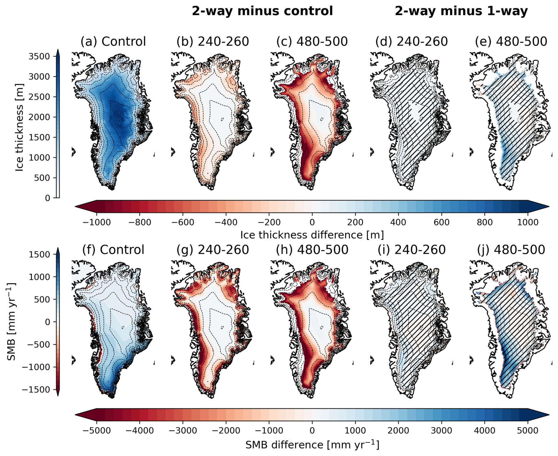
Figure A1 Ice thickness [m] and surface mass balance (SMB) [mm yr⁻¹] as downscaled to the CISM2 grid (4 km) for (a, f) the mean of the control simulation, (b, c, g, h) anomalies of the two-way coupled simulation with respect to the control simulation and (d, e, i, j) anomalies of the two-way with respect to the one-way coupled simulation for grid points that have not deglaciated in both simulations, for (b, d, g, i) the years 240–260 and (c, e, h, j) the years 480–500. The dashed black lines depict contour lines for every 500 m of elevation of the control (a, f) and two-way coupled (b–e, g–j) simulations. Hatches denote areas in which the differences between the one- and two-way coupled simulations have not become significant before the last year of the corresponding period. Because of a different evolution of ice sheet topography, the two simulations show a different SMB pattern, leading to a few locations in which the one-way simulation shows less SMB reduction.

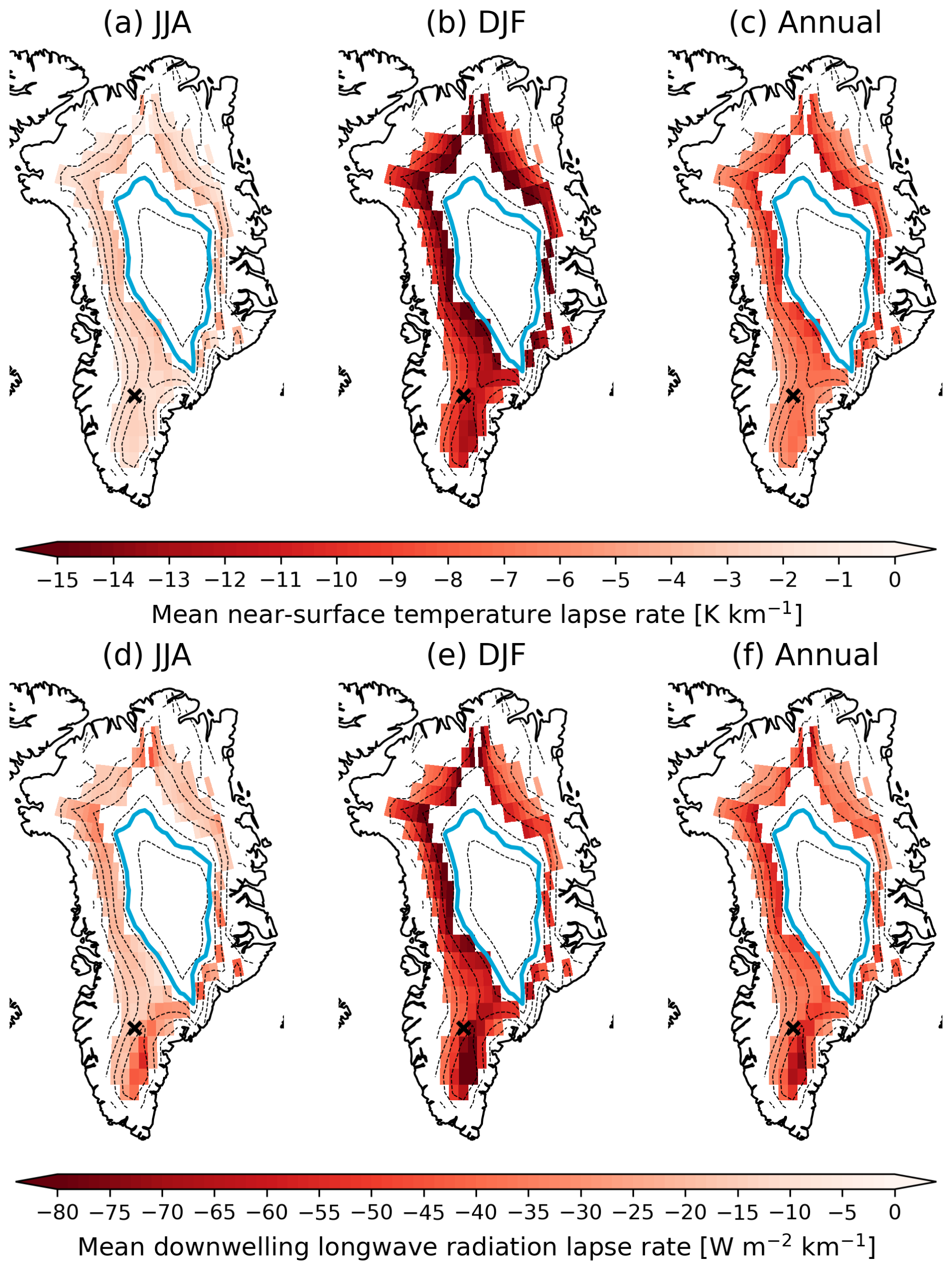
Figure A2 Lapse rate of (a–c) near-surface (2 m) air temperature [K km⁻¹] and (d–f) downwelling shortwave radiation [$\mathrm{W}{\mathrm{m}}^{-\mathrm{2}}{\mathrm{km}}^{-\mathrm{1}}$] for (a, d) June–July–August (JJA) mean, (b, e) December–January–February (DJF) mean and (c, f) annual mean. The black lines depict contour lines for every 500 m elevation of the two-way simulation. The light blue line represents the ELA of the two-way simulation. The black cross shows the location of the point shown in Fig. 5.

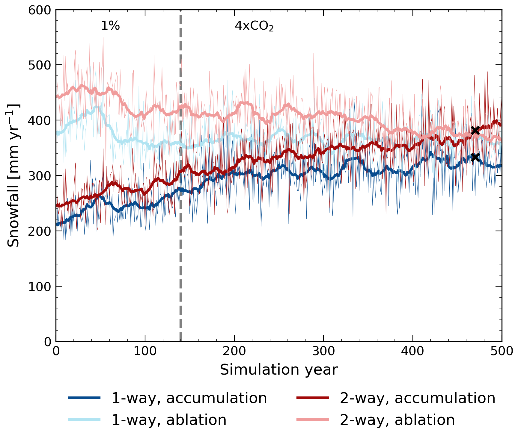
Figure A3 Evolution of snowfall [mm yr⁻¹] in the one-way (blue) and two-way (red) coupled simulation for the end-of-simulation ablation and accumulation area. The dashed grey line indicates the end of the 1 % CO₂ ramp-up period and the start of the continuous 4×CO₂ period. If the differences between the one- and two-way coupled simulations become significant throughout the simulation, the first year of significant difference is marked with a black cross.

Appendix B: CO₂ reduction

Table B1 Year of recovery. In case the variable has not recovered by the end of the simulation (year 925), the remaining anomaly of the mean state of the variable in the last 100 years of the simulation with respect to the closest boundary of the 1σ confidence interval is computed, as well as the remaining linear trend over the last 100 years. A positive anomaly means that the end-of-simulation state of the variable is larger than in the control simulation. If the trend and remaining anomaly are in the opposite direction, an extrapolated recovery year is given. The relative amount of recovery [%] is given for variables that have not recovered by the end of the simulation.

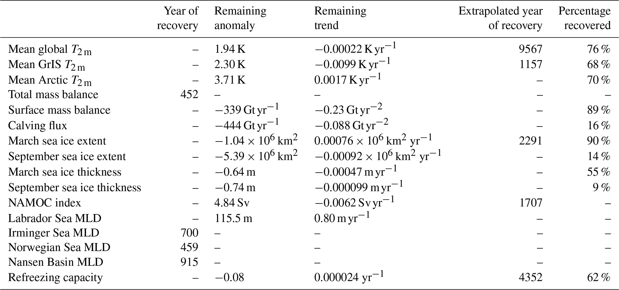
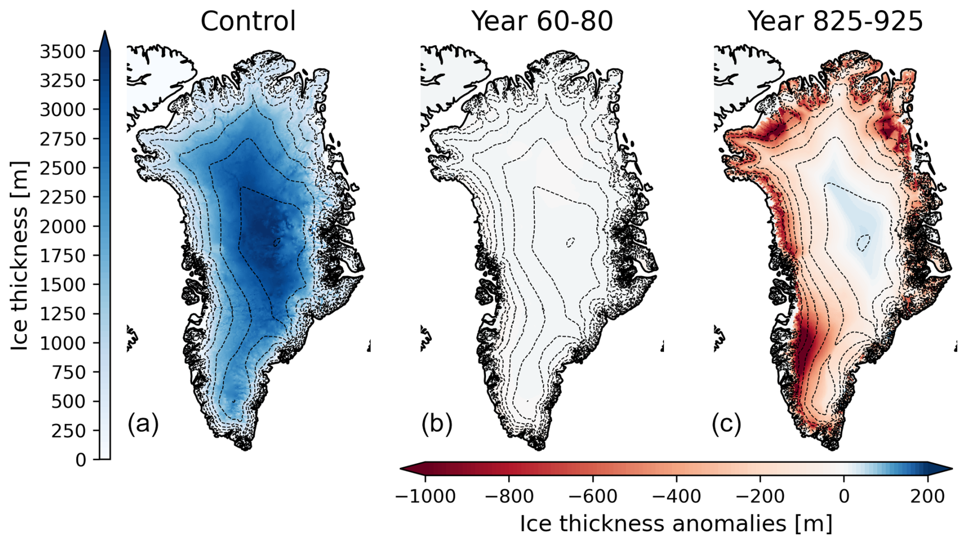
Figure B1 Ice thickness [m] downscaled to the CISM2 grid (4 km) for (a) the mean of the control simulation, (b) the anomalies of the CO₂ reduction simulation with respect to the control simulation in year 70 (60–80 mean) and (c) the same as in (b) for the end of the simulation (year 825–925).

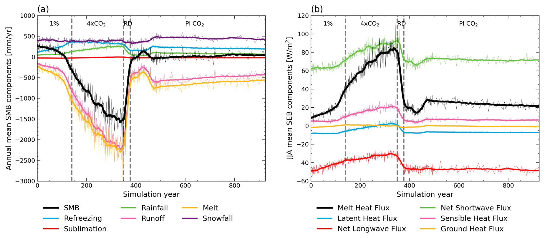
Figure B2 Evolution of (a) GrIS annual mean SMB [mm yr⁻¹] and its components and (b) GrIS JJA (June, July, August) mean SEB [W m⁻²] and its components for the simulation in which we reintroduce PI CO₂. The dashed grey lines indicate the end of the 1 % CO₂ ramp-up, the continuous 4×CO₂, the ramp-down (RD) to PI CO₂ and the continuous PI CO₂ periods.

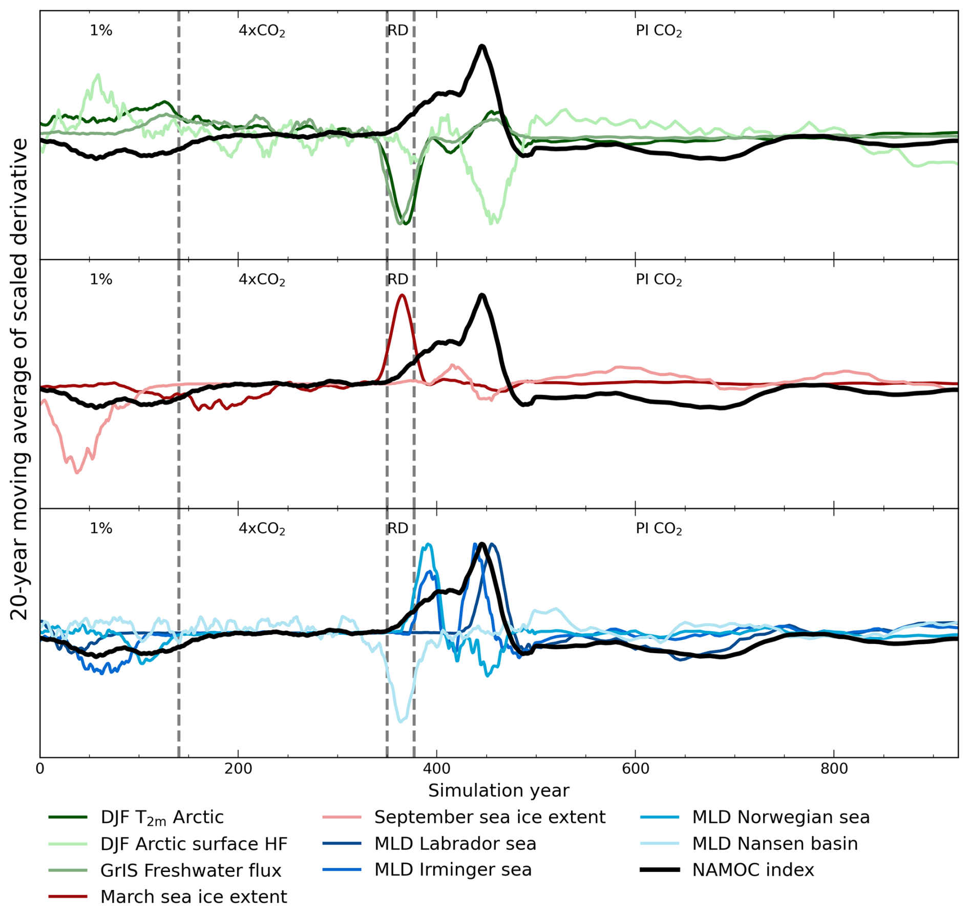
Figure B3 The 20-year moving average of the derivative of processes interacting with the NAMOC (black). These are the winter Arctic T_2 m; the winter Arctic surface heat flux; the GrIS freshwater flux; the March and September sea ice extent; and the winter MLDs in the Labrador Sea, Irminger Sea, Norwegian Sea and Nansen Basin. The derivatives are computed using the central difference method and thereafter scaled to their maximum response. The dashed grey lines indicate the end of the 1 % CO₂ ramp-up, the continuous 4×CO₂, the ramp-down (RD) to PI CO₂ and the continuous PI CO₂ periods.

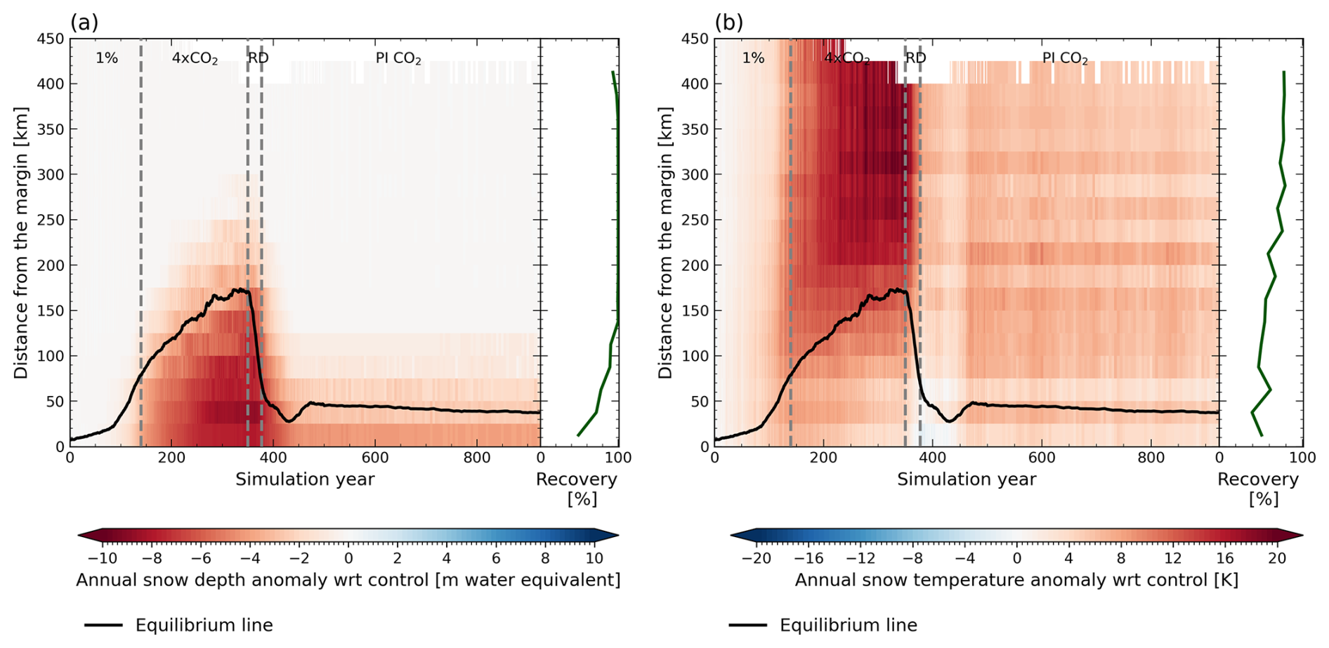
Figure B4 Anomalies of (a) annual mean snow depth [$\mathrm{m}\mathrm{w}.\mathrm{e}.$] and (b) annual mean snow temperature [K] over the GrIS with respect to the control mean as a function of time and distance to the ice sheet margin for the reintroduction of PI CO₂ simulation. The black line denotes the mean distance of the equilibrium line to the margin, and the dark green line shows the relative recovery (in %) for each distance class. The dashed grey lines indicate the end of the 1 % CO₂ ramp-up, the continuous 4×CO₂, the ramp-down (RD) to PI CO₂ and the continuous PI CO₂ periods.