Satellite data reveal details of glacial isostatic adjustment in the Amundsen Sea Embayment, West Antarctica

The instability of the West Antarctic Ice Sheet (WAIS) is a tipping element in the climate system, and it is mainly dictated by changes in the ice flow behaviour of the outflow glaciers in the Amundsen Sea Embayment (ASE). Recent studies postulated that the vertical uplift of bedrock can delay the collapse of glaciers in this region. In West Antarctica, bedrock motion is largely caused by a fast viscoelastic response of the upper mantle to changes in ice loads over the last centuries. This glacial isostatic adjustment (GIA) effect is currently poorly understood, since Earth's rheology and the ice-loading history are both subject to large uncertainties in simulations. Moreover, results from data-driven approaches have not yet resolved GIA at a sufficient spatial resolution. We present a data-driven GIA estimate, based on data from GRACE/GRACE-FO (GRACE and GRACE-FO), CryoSat-2 altimetry, regional climate modelling, and firn modelling, which is the first to agree with independent vertical velocities in West Antarctica derived from global navigation satellite system (GNSS) data. Our data combination yields a maximum GIA bedrock motion rate of 43 ± 7 mm a⁻¹ in the Thwaites Glacier region and agrees within uncertainties in the GNSS-derived rate. The data-driven GIA-related bedrock motion may be used in future simulation runs to quantify a potential delay of the collapse of the West Antarctic Ice Sheet due to the stabilization effects induced by GIA. Furthermore it may be used for testing rheological models with low upper-mantle viscosity in conjunction with centennial loading histories.

1 Introduction

The shrinking of ice sheets due to a warming climate and its contribution to sea level rise is a major public concern. The West Antarctic Ice Sheet (WAIS) warrants particular focus because, if the global mean temperature exceeds 1.5 °C relative to the pre-industrial period, a threshold may be reached at which the WAIS becomes unstable (McKay et al., 2022). The instability means that the glacier flow accelerates abruptly, leading to a major outflow of ice from the WAIS into the ocean. This 1.5 °C threshold is very likely to be reached within the next 20 years, even considering low-emission scenarios (IPCC, 2021). Furthermore, ice–ocean interaction simulations demonstrated that any reduction in greenhouse gases has a very limited impact on preventing WAIS' accelerated contribution to sea level rise over the next decades (Naughten et al., 2023).

A changing bedrock topography due to solid-Earth deformation may affect the glacier flow and thus the outflow flux (Whitehouse et al., 2019). High bedrock uplift rates of several centimetres per year in the region of the Amundsen Sea Embayment (ASE) are evident from global navigation satellite system (GNSS) measurements (Groh et al., 2012), and this uplift may provide a feedback that stabilizes the WAIS in the future (Adhikari et al., 2014; Gomez et al., 2015, 2024; Konrad et al., 2015; Book et al., 2022). Namely, bedrock uplift leads to a shift in the grounding line – the boundary between the grounded ice on the continent and the floating ice – towards the ocean. If the grounding line moves towards the ocean, a larger part of the glacier ice will be grounded on the continent and the ice thickness at the grounding line will be smaller. A smaller ice thickness results in less ice outflow, resulting in a stabilization of the ice sheet (Whitehouse et al., 2019). The GNSS observations that provide estimates for this bedrock uplift are subject to limitations: in particular, a restriction to bedrock outcrops leading to a coarse spatial sampling and expensive logistics, with the consequence that many sites have low temporal sampling, too. Barletta et al. (2018) modelled glacial isostatic adjustment (GIA) to fit the high bedrock uplift rates observed with GNSS in the ASE. They show that the GNSS observations can be explained by a mantle response to ice changes in the last 100 years when adopting very low upper-mantle viscosity. Global 1D GIA models only barely explain the observed uplift rate in the ASE, as they typically utilize a rheology and an ice-loading history that are outside the range of parameters relevant to this region (Whitehouse et al., 2019).

For the Antarctic Ice Sheet, there is considerable difference amongst various models of present-day GIA and its induced mass effect (Whitehouse et al., 2019). To elucidate: Groh and Horwath (2021) estimate a gravimetric ice mass balance of the Antarctic Ice Sheet (AIS) of −91 ± 44 Gt a⁻¹ from April 2002 until July 2020. The uncertainty in the present-day GIA mass effect contributes to about three-quarters of the indicated total mass balance uncertainty (Groh and Horwath, 2021). Data combination approaches, often called inverse approaches, estimate the GIA-induced mass changes by utilizing satellite gravimetry and satellite altimetry observations. These GIA estimates are useful for improving the ice mass change (IMC) estimates of the AIS (Willen et al., 2024). However, published inverse GIA estimates that do not incorporate GNSS data explain only a part of the bedrock uplift in the ASE. These approaches resolve GIA at a coarse spatial resolution only, at a level that is insufficient to explain the GNSS observations in the ASE (for an overview, see Whitehouse et al., 2019). For example, combination approaches from Riva et al. (2009), Gunter et al. (2014), Engels et al. (2018), and Willen et al. (2024) can only resolve GIA at an effective spatial resolution of >400 km, which is insufficient to capture the GIA effect with spatial scales of ∼100 km as postulated by Barletta et al. (2018). This coarse resolution is mainly a consequence of processing choices informed by the data quality. The shortcoming that explains the GNSS-derived uplift magnitudes and small spatial scales also holds for the inverse approaches that incorporate GNSS data in addition to gravimetry and altimetry data (Martín-Español et al., 2016b, a; Sasgen et al., 2017). Furthermore, including GNSS data directly in the inversion removes the ability to independently validate GIA estimates.

So far it has not been possible to resolve GIA-related bedrock motion in the ASE at a realistic order of magnitude independently from GNSS measurements. Here, we investigate how we can quantify a realistic GIA with observations spatially continuously covering the whole ASE. Given the high signal-to-noise ratio in the ASE region and improved data processing, we hypothesize that a data combination approach on the time series level can achieve this. We develop this combination approach according to Willen et al. (2020), who builds upon the approach of Gunter et al. (2014), while we avoid unrealistic spatial-scale constraints. By that, we can provide a spatially continuous description of GIA in the ASE that supplements the sparse sampling of GNSS-based GIA estimates. To do so, we make use of 10 years of available elevation changes from CryoSat-2 data, gravitational field changes from GRACE/GRACE-FO (GRACE and GRACE-FO), and regional climate modelling (RACMO2) as well as firn modelling (IMAU-FDM, Institute for Marine and Atmospheric research Utrecht firn densification model) outputs. We restrict the analysis here to the elevation changes in CryoSat-2 because earlier altimetry missions have either a limited spatial sampling by orbit design (Envisat) or a limited temporal sampling by mission concept (ICESat). In addition, CryoSat-2 offers high data quality (Schröder et al., 2017). Thereby we accept being limited to a time span of 10 years. We use GNSS data only to validate our GIA estimate and do not include it in the estimation procedure.

2 Data

Our data combination approach uses data from the GRACE and GRACE-FO satellite missions. These are monthly gravity field changes (Sect. 2.1). Next, it includes monthly grids of elevation changes derived from the radar altimetry mission CryoSat-2 (Sect. 2.2). Lastly, the approach incorporates modelling outputs from the regional climate model RACMO2 and the firn model IMAU-FDM. More precisely, the data combination uses monthly changes in firn air content (FAC) derived from the modelling outputs (Sect. 2.3). The firn layer of an ice sheet can be conceptually divided into two components: ice and air. FAC represents the air component, expressed as an equivalent height. Section 3 details how FAC relates to the observations and how the combination approach includes FAC. The use of FAC over firn density benefits a data combination approach, as previously demonstrated by Willen et al. (2022). GNSS data serve to validate the results (Sect. 2.4). All datasets are available with at least monthly temporal resolution. With regard to GIA-related deformation, such a high temporal resolution is presumably not necessary. However, we combine the datasets at a monthly temporal resolution, as we do not aim here to implement any a priori assumptions about the temporal behaviour of the signals. All of the following subsections describe how we use monthly uncertainty information from the datasets. In all cases where we provide rate estimates, the corresponding rate uncertainty follows from a full error covariance propagation using the analogous data combination on the trend level. We use the error covariances of all input datasets from Willen et al. (2022) to estimate rate uncertainties.

2.1 Satellite gravimetry

We utilize ITSG-Grace2018 and ITSG-Grace_op monthly gravity field solutions up to degree and order 96 (Mayer-Gürr et al., 2018). Ditmar (2022) found that these solutions outperform other gravity field solutions in terms of noise level and signal retainment. Spherical harmonic coefficients of degree 1 complement the gravitational field, following the approach from Sun et al. (2016). We thus transfer the gravity fields into a centre-of-figure reference frame. We replace (i) the spherical harmonic coefficient of degree 2 and order 0 with satellite laser ranging products (Loomis et al., 2020) for all gravitational fields and (ii) the coefficient of degree 3 and order 0 for gravitational fields obtained during GRACE/GRACE-FO accelerometer failures. We express these gravitational field changes as surface density changes (Eq. 3) on the WGS84 ellipsoidal surface, applying the approach from Ditmar (2018), and transfer them to the spatial domain on a 20 km×20 km polar stereographic grid in West Antarctica (Fig. 1a).

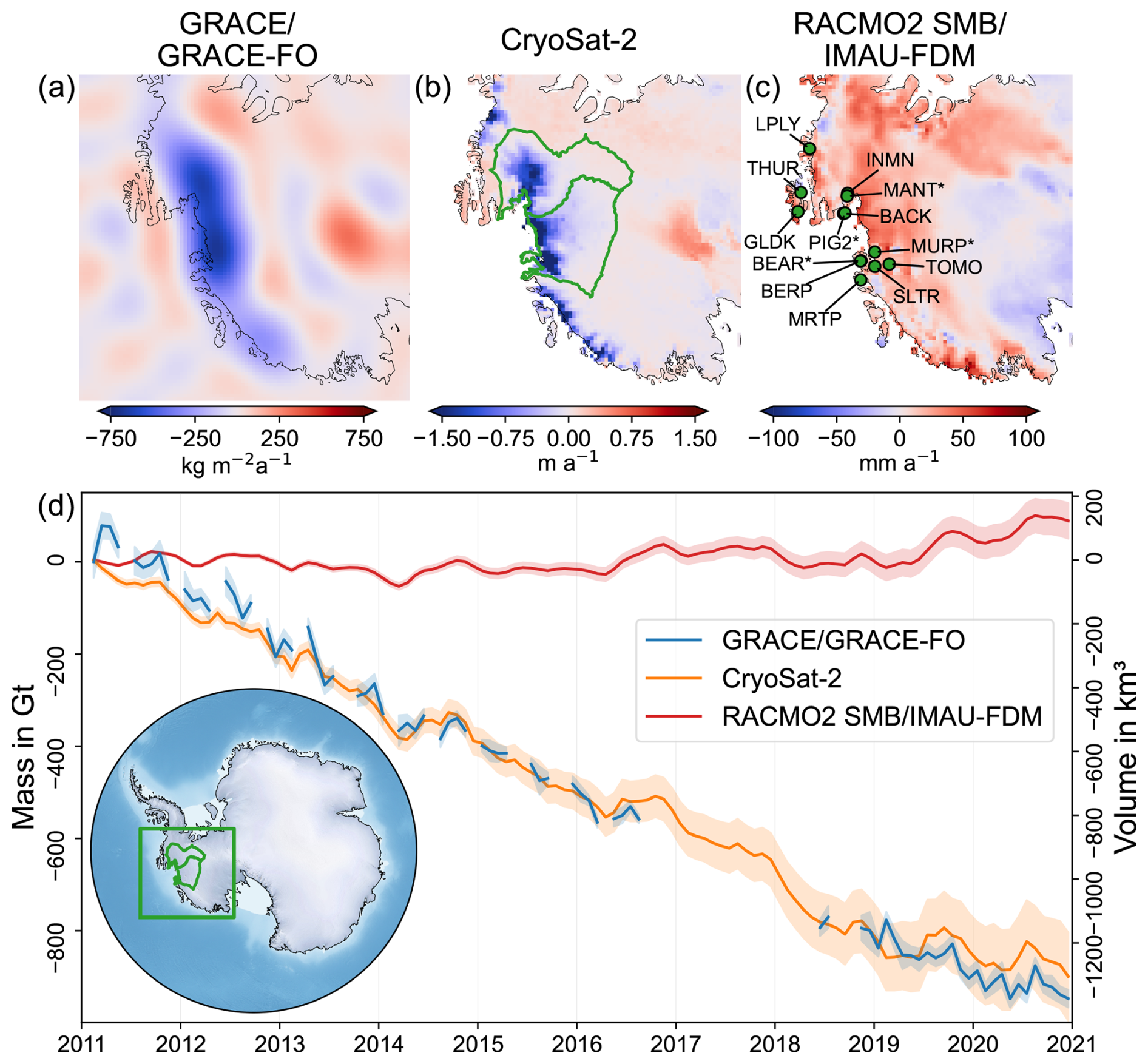
Figure 1 The original input data in the study region. Mean rates from January 2011 to December 2020 of (a) surface density rates from GRACE/GRACE-FO data (Mayer-Gürr et al., 2018), (b) surface elevation rates from CryoSat-2 (Helm et al., 2014, 2024), and (c) the firn air content (FAC) from IMAU-FDMv1.2A (Veldhuijsen et al., 2023) and RACMO2.3p2 SMB (van Wessem et al., 2018) (c). GNSS site locations where data are used for validation purposes are illustrated with green circles and labelled with site names in (c) (see Table 1). The asterisk (*) indicates sites that have only been observed episodically. The drainage area of the Amundsen Sea Embayment (ASE), i.e. basin 21 and 22 according to Zwally et al. (2012), is indicated with a green polygon in (b). (d) Time series of integrated observations over the ASE region including an overview of the investigation area. Left y axis: mass change (GRACE/GRACE-FO); right y axis: volume change (CryoSat-2 and RACMO2 SMB–IMAU-FDM).

We propagate the full error covariance information (Koch, 1999) provided along with the ITSG monthly gravity field solutions (Mayer-Gürr et al., 2018) to the spatial domain, i.e. to the surface density changes using the ellipsoidal surface approximation. Gaussian smoothing suppresses the typical spatially correlated GRACE/GRACE-FO error patterns. A full propagation of the spatially correlated errors is certainly the most complete approach, yet it leads to very high computational efforts. Therefore, on the time series level of the data combination, we simplify the error propagation and restrict ourselves to the spatially uncorrelated error parts. Our error estimates thus serve as an upper bound.

2.2 Satellite altimetry

We obtain monthly grids of surface elevation changes from CryoSat-2 data processed using an updated approach according to Helm et al. (2014); i.e. the elevation change is derived using a threshold first-maximum retracking algorithm (TFMRA) retracker and corrected with sigma correlation (cf. Sect. 2.4 in Helm et al., 2024). We resample the surface elevation changes to the same 20 km×20 km polar stereographic grid in West Antarctica that we use for evaluation of GRACE/GRACE-FO data in the spatial domain.

As there is no official uncertainty product, we assess the uncertainty in the surface elevation time series by comparing data from CryoSat-2 and ICESat-2 during the 4-year period from January 2019 to December 2022, when both altimetry missions were observing simultaneously. We assume two types of uncertainties: (1) temporally uncorrelated, i.e. white noise, and (2) temporally correlated over the full observation period, i.e. a trend uncertainty. The uncorrelated uncertainty (1) is quantified by the standard deviation of the residuals that result by fitting a deterministic trend-cycle model (bias, linear, quadratic, annual cycles, semi-annual cycles) to CryoSat-2 and ICESat-2 differences. We quantify the trend uncertainty (2) by calculating the rate and the acceleration of differences between CryoSat-2 and ICESat-2. This trend uncertainty is relative to January 2011; i.e. at this time, the trend uncertainty is 0 and increases over time.

2.3 Firn air content (FAC) changes

To obtain the time series of the FAC change (e.g. Ligtenberg et al., 2014), we use an updated version of the RACMO2.3p2 surface mass balance (SMB) output (retrieved on 30 November 2021; van Wessem et al., 2018) and firn thickness changes from IMAU-FDM v1.2A (Veldhuijsen et al., 2023). We assume that the mass change in the firn layer equals the SMB change. From the firn thickness change and SMB, we calculate the change in FAC (Eq. 6). Similar to the previous datasets, FAC changes are resampled to the same 20 km×20 km polar stereographic grid.

We characterize the uncertainty in the FAC time series using an alternative FAC product from the Goddard Space Flight Center (GSFC), GSFC-FDM (Medley et al., 2022), for comparison. Here, we also assume two types of uncertainties: uncorrelated in time and fully correlated in time over the observation period. For quantification, we follow the same approach that we apply to surface elevation changes from satellite altimetry (Sect. 2.2). To do so, we evaluate differences in FAC changes from IMAU-FDM and GSFC-FDM.

2.4 GNSS data

The GNSS data originate from sites in Antarctica with GNSS antennas mounted on bedrock outcrops, directly observing horizontal and vertical bedrock displacement. The data combination method (Sect. 3) only allows for the estimation of vertical bedrock motion, so we do not consider horizontal displacements further. There are two different GNSS setups to monitor bedrock motion. These include (1) continuous sites (cont in Table 1), which are designed to enable continuous measurements over several years. On the other hand, there are (2) episodic sites (epis in Table 1), at which recurring campaign measurements are realized at fixed anchored locations. The campaigns are repeated after several years, with data usually being collected over several days in each individual campaign (Scheinert et al., 2021). With continuous sites (1) the motion of the surface of the solid Earth can be studied at a high temporal resolution. The campaign-style experiments (2) aim by design to only provide long-term rates of bedrock motion. Some sites were initially designed as episodic setups and were later upgraded to continuously operating sites (both in Table 1).

Table 1 Overview of used GNSS data in the Amundsen Sea Embayment that were analysed by Buchta et al. (2024). The first four columns provide the GNSS site ID, their coordinates (long and lat), and the type of GNSS observations (continuous (cont) site or an episodic (epis) site or a mixture of both (both)). The fifth column gives the number of campaigns (NOC). The columns labelled “Start” and “End” list when the first and last observations were taken. The column labelled “Duration” specifies the total time span rounded to full years. Vertical bedrock motion rates and their split into the elastic-related and GIA-related component (Eq. 11) are provided in the columns labelled “${\dot{h}}^{\mathsf{\text{bm}}}$”, “${\dot{h}}^{\mathsf{\text{ela}}}$”, and “${\dot{h}}^{\mathsf{\text{gia}}}$”, respectively.

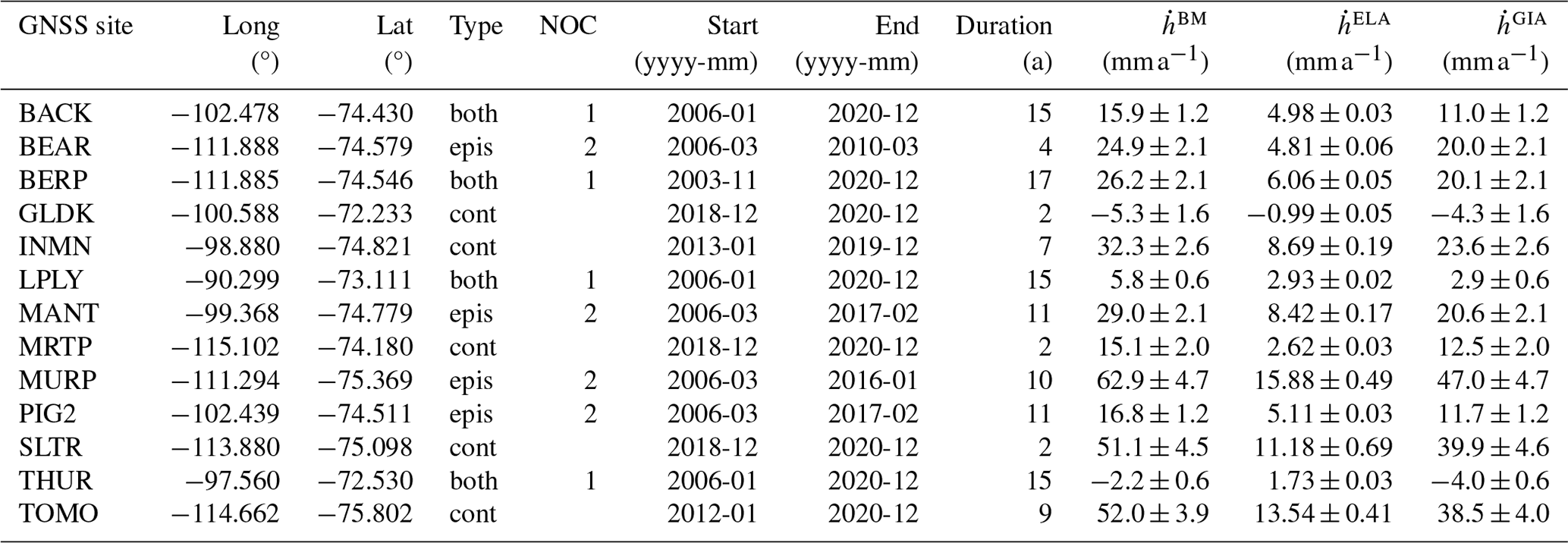
We include 13 GNSS sites in this study. The sites are either affiliated with the POLENET-ANET network (Wilson et al., 2019) or result from measurement campaigns conducted by TU Dresden (Technische Universität Dresden). The GNSS-derived bedrock motions result from a consistent Antarctica-wide analysis that has been accomplished in the frame of the SCAR-endorsed Geodynamics In ANTarctica based on REprocessing GNSS dAta INitiative (GIANT-REGAIN; Buchta et al., 2024). Here we use the processing results of the individual TU Dresden solution. The GNSS data are in centre-of-figure reference frame IGb14. We refer the reader to Buchta et al. (2024) for all details of GNSS data processing. For each month, m, we calculate the weighted mean of all daily solutions in that month:

$$\begin{array}{}\text{(1)}& {\displaystyle }{\displaystyle }{h}_m^{\mathsf{\text{gnss}}}={\displaystyle \frac{{\sum }_{d=\mathrm{1}}^D{h}_d^{\mathsf{\text{gnss}}}({\mathit{\sigma }}_d^{\mathsf{\text{gnss}}}{)}^{-\mathrm{2}}}{{\sum }_{d=\mathrm{1}}^D({\mathit{\sigma }}_d^{\mathsf{\text{gnss}}}{)}^{-\mathrm{2}}}},\end{array}$$

where $h_d^{\mathsf{\text{gnss}}}$ and ${\mathit{\sigma }}_d^{\mathsf{\text{gnss}}}$ refer to the GNSS-derived vertical component available at a day, d, and its uncertainty, respectively. D is the number of available daily solutions in a certain month, m.

The uncertainty in the monthly weighted averages, ${\mathit{\sigma }}_m^{\mathsf{\text{gnss}}}$, could be calculated from the formal daily uncertainties (e.g. Taylor, 1997, Chap. 7). However, we find unphysical scatter of the daily values within a month that is not represented by the formal uncertainties in each daily solution. From this we conclude that the formal uncertainties are likely to be over-optimistic and too limited to represent all noise sources (Buchta et al., 2024). For this reason, we add a measure of the scatter of all daily solutions within a month, i.e. their variance, as an additional measure of uncertainty to the formal uncertainties:

$$\begin{array}{ll}{\displaystyle }({\mathit{\sigma }}_m^{\mathsf{\text{gnss}}}{)}^{\mathrm{2}}=& {\displaystyle }{\left[\sum _{d=\mathrm{1}}^D({\mathit{\sigma }}_d^{\mathsf{\text{gnss}}}{)}^{-\mathrm{2}}\right]}^{-\mathrm{1}}\\ \text{(2)}& {\displaystyle }& {\displaystyle }+{\displaystyle \frac{\mathrm{1}}{D-\mathrm{1}}}\sum _{d=\mathrm{1}}^D(h_d^{\mathsf{\text{gnss}}}-h_m^{\mathsf{\text{gnss}}}{)}^{\mathrm{2}}.\end{array}$$

The first summand represents the uncertainty in the weighted mean derived from the formal daily uncertainties. The second summand is the variance of the daily expectation values within a month.

3 Regional data combination method

In order to quantify GIA-related bedrock motion and GIA-related gravity changes in the ASE, we apply a data combination method similar to the method presented by Gunter et al. (2014) and that was extended to a combination on the time series level by Willen et al. (2020). We utilize observations of satellite gravimetry and satellite altimetry as well as results of regional climate modelling and firn modelling (Sect. 2). Further we use GNSS data for validation. Signals to be separated are from the GIA and IMC processes. The data combination method builds upon the different sensitivity of the datasets towards the signals to be separated. This sensitivity is given by the effective densities between the physical quantities that change due to the processes explained below. We aim to solve for the physical quantity of bedrock motion that contemporary changes due to GIA (h^𝙜𝙞𝙖), and we co-estimate the surface density change due to IMC (κ^𝙞𝙢𝙘).

3.1 Surface density changes

Time series of monthly surface density changes, κ, with the unit $\left[\mathit{\kappa }\right]=\mathrm{kg}{\mathrm{m}}^{-\mathrm{2}}{\mathrm{a}}^{-\mathrm{1}}$, loosely also referred to as mass changes, derived from satellite gravimetry, κ^{𝙜𝙧𝙖𝙫}, contain the following quantities:

$$\begin{array}{}\text{(3)}& {\displaystyle }{\displaystyle }{\mathit{\kappa }}^{\mathsf{\text{grav}}}={\mathit{\kappa }}^{\mathsf{\text{gia}}}+{\mathit{\kappa }}^{\mathsf{\text{imc}}}+{\mathit{\kappa }}^{\mathsf{\text{other}}}+{\mathit{\epsilon }}^{\mathsf{\text{grav}}},\end{array}$$

where κ^{𝙜𝙧𝙖𝙫} originates from monthly gravitational fields provided as Stokes coefficients and is evaluated on an ellipsoidal surface to retrieve surface density changes (Ditmar, 2018). The potential change related to elastic deformation is accounted for when converting potential changes to surface density changes. κ^𝙜𝙞𝙖 and κ^𝙞𝙢𝙘 are surface density changes related to GIA and IMC, respectively. κ^{𝙤𝙩𝙝𝙚𝙧} refers to far-field effects from mass changes from all other regions on Earth that result from the evaluation of gravitational field changes (Willen et al., 2024). In the ASE, we assume that these far-field effects are very small compared to the mass variations taking place in the ASE and can be neglected. ε^{𝙜𝙧𝙖𝙫} refers to the observational error in satellite gravimetry.

Ice mass change (IMC), κ^𝙞𝙢𝙘, is the sum of mass changes in the firn layer, κ^{𝙛𝙞𝙧𝙣}, and in the ice layer, κ^𝙞𝙘𝙚. Mass changes in the firn layer are explained by the surface mass balance (SMB), e.g. modelled with a regional climate model (Sect. 2). We assume that κ^{𝙛𝙞𝙧𝙣}∼κ^𝙨𝙢𝙗:

$$\begin{array}{}\text{(4)}& {\displaystyle }{\displaystyle }{\mathit{\kappa }}^{\mathsf{\text{imc}}}={\mathit{\kappa }}^{\mathsf{\text{smb}}}+{\mathit{\kappa }}^{\mathsf{\text{ice}}}.\end{array}$$

3.2 Surface elevation changes

Time series of surface elevation changes, h, with the unit $\left[h\right]={\mathrm{m}\mathrm{a}}^{-\mathrm{1}}$, observed with satellite altimetry, h^𝙖𝙡𝙩, contain the following signals:

$$\begin{array}{}\text{(5)}& {\displaystyle }{\displaystyle }{\mathit{h}}^{\mathsf{\text{alt}}}={\mathit{h}}^{\mathsf{\text{imc}}}+{\mathit{h}}^{\mathsf{\text{fac}}}+{\mathit{h}}^{\mathsf{\text{gia}}}+{\mathit{h}}^{\mathsf{\text{ela}}}+{\mathit{\epsilon }}^{\mathsf{\text{alt}}},\end{array}$$

where h^𝙜𝙞𝙖 and h^𝙚𝙡𝙖 refer to GIA-induced and elastic-deformation-induced bedrock motion, respectively. h^𝙞𝙢𝙘 is the surface elevation change due to IMC. h^𝙛𝙖𝙘 refers to the change in firn air content (FAC):

$$\begin{array}{}\text{(6)}& {\displaystyle }{\displaystyle }{\mathit{h}}^{\mathsf{\text{fac}}}={\mathit{h}}^{\mathsf{\text{firn}}}-{\displaystyle \frac{{\mathit{\kappa }}^{\mathsf{\text{smb}}}}{{\mathit{\rho }}^{\mathsf{\text{ice}}}}}.\end{array}$$

We obtain h^𝙛𝙖𝙘 from modelled firn thickness variations (Sect. 2), h^{𝙛𝙞𝙧𝙣}, and express the modelled cumulated SMB anomalies as a purely solid-ice-related elevation change. ρ^𝙞𝙘𝙚 is the density of pure ice and is assumed to be 917 kg m⁻³. Thereby we assume that the sum of elevation changes due to IMC and FAC (h^𝙞𝙢𝙘+h^𝙛𝙖𝙘) equals the sum of surface elevation changes caused by changes in ice flow dynamics and firn thickness (h^𝙞𝙛𝙙+h^{𝙛𝙞𝙧𝙣}).

3.3 Combining surface elevation and surface density changes

The ratio of the surface density change and the surface elevation change caused by GIA has the unit of a density and is referred to as the effective GIA density, ρ^𝙜𝙞𝙖:

$$\begin{array}{}\text{(7)}& {\displaystyle }{\displaystyle }{\mathit{\kappa }}^{\mathsf{\text{gia}}}={\mathit{\rho }}^{\mathsf{\text{gia}}}{\mathit{h}}^{\mathsf{\text{gia}}}.\end{array}$$

We use a spatial mask given the GIA density at each location in Antarctica similar to the one utilized by Riva et al. (2009). They assessed this ratio between GIA-induced gravity changes and GIA-induced geometry changes from GIA forward model outputs following findings from Wahr et al. (2000) and refined it to account for the self-gravitation of sea level. Following Riva et al. (2009), we generate the mask by assuming ${\mathit{\rho }}_{\mathsf{\text{continent}}}^{\mathsf{\text{gia}}}=\mathrm{4000}\mathrm{kg}{\mathrm{m}}^{-\mathrm{3}}$ over the continent and ${\mathit{\rho }}_{\mathsf{\text{ocean}}}^{\mathsf{\text{gia}}}=\mathrm{3400}\mathrm{kg}{\mathrm{m}}^{-\mathrm{3}}$ over the ocean. We assume a smooth transition between the continent and ocean by using a 100 km Gaussian smoother (Fig. S2 in the Supplement). Note that we do not run GIA forward models to tune these densities, nor the length of transition between continent and ocean. Riva et al. (2009) found that a 300 kg m⁻³ increase in the GIA density leads to an 2.5 % increase in the GIA solution. Using Eq. (7) and the relation

$$\begin{array}{}\text{(8)}& {\displaystyle }{\displaystyle }{\mathit{\kappa }}^{\mathsf{\text{imc}}}={\mathit{\rho }}^{\mathsf{\text{ice}}}{\mathit{h}}^{\mathsf{\text{imc}}}\end{array}$$

while leaving out the error components, we deterministically combine surface density changes and elevation changes as follows to separate GIA-related surface density changes and surface elevation changes, respectively:

$$\begin{array}{}\text{(9)}& {\displaystyle }& {\displaystyle }{\mathit{h}}^{\mathsf{\text{gia}}}=\left({\mathit{h}}^{\mathsf{\text{alt}}}-{\mathit{h}}^{\mathsf{\text{fac}}}-{\mathit{h}}^{\mathsf{\text{ela}}}-{\displaystyle \frac{{\mathit{\kappa }}^{\mathsf{\text{grav}}}}{{\mathit{\rho }}^{\mathsf{\text{ice}}}}}\right){\displaystyle \frac{{\mathit{\rho }}^{\mathsf{\text{ice}}}}{{\mathit{\rho }}^{\mathsf{\text{ice}}}-{\mathit{\rho }}^{\mathsf{\text{gia}}}}}\text{(10)}& {\displaystyle }& {\displaystyle }{\mathit{\kappa }}^{\mathsf{\text{gia}}}={\mathit{\rho }}^{\mathsf{\text{gia}}}\cdot {\mathit{h}}^{\mathsf{\text{gia}}}.\end{array}$$

This assumes that κ^{𝙤𝙩𝙝𝙚𝙧}=0 in Eq. (3) as mentioned above. We approximate ${\mathit{h}}^{\mathsf{\text{alt}}}-{\mathit{h}}^{\mathsf{\text{fac}}}-{\mathit{h}}^{\mathsf{\text{ela}}}$ with 1.015(h^𝙖𝙡𝙩−h^𝙛𝙖𝙘) (Riva et al., 2009).

The GIA-related mean rate of surface density changes and surface elevation changes, ${\dot{\mathit{\kappa }}}^{\mathsf{\text{gia}}}$ and ${\dot{h}}^{\mathsf{\text{gia}}}$, respectively, can be obtained from κ^𝙜𝙞𝙖 and h^𝙜𝙞𝙖 via least-squares adjustment of a trend-seasonal model. Co-estimated seasonal (annual and semi-annual) components capture potential errors that have propagated to the GIA result.

The error covariance information from Willen et al. (2024) for the mean rates of the input datasets provides more realistic error information than what is available for data on the time series level. To estimate more realistic uncertainties in the estimated GIA-related mean rates, we adapt the time series combination approach (Eq. 9) to a trend-level combination approach as in Gunter et al. (2014). To do so, one needs to first determine the mean rates from a least-squares adjustment of the input datasets (${\dot{h}}^{\mathsf{\text{alt}}}$, ${\dot{h}}^{\mathsf{\text{fac}}}$, ${\dot{\mathit{\kappa }}}^{\mathsf{\text{grav}}}$) and then combine these analogically as shown in Eq. (9) to estimate ${\dot{\mathit{\kappa }}}^{\mathsf{\text{gia}}}$ and ${\dot{h}}^{\mathsf{\text{gia}}}$. Note that we use the combination on the trend level only for propagating error covariances.

3.4 Optimal spatial unification of input data

To unify the spatial resolution of the input data (Gunter et al., 2014), we first apply a Gaussian smoother to each dataset. This step is most likely legitimate for determining GIA effects, as these occur at longer spatial wavelengths than the resolution of satellite altimetry (<10 km). According to modelling results from Barletta et al. (2018), even GIA associated with low viscosity in the upper mantle and centennial ice-loading changes occur on spatial wavelengths larger than 100 km (cf. Fig. S13 in Barletta et al., 2018). However, IMC takes place on much smaller spatial scales. By combining previously smoothed data, we can only determine a spatially smoothed κ^𝙞𝙢𝙘.

It is initially unknown what Gaussian filter width (here referred to as the half-response width, i.e. the distance between the maximum and its half amplitude) is optimal for separating GIA from IMC such that the spatial resolution is close to the true GIA effect. If the filter width is too large, the true GIA signal may be overly smoothed. A filter width that is too small may lead to insufficient unification of the spatial resolution so that the result is dominated by artefacts and spatial noise. To identify what filter width is optimal, we compare the GIA-related bedrock motion from the combination (Eq. 9) with independent GNSS data. GNSS observations, h^{𝙜𝙣𝙨𝙨}, observe the full bedrock motion, h^𝙗𝙢, which contains both GIA and elastic contributions:

$$\begin{array}{}\text{(11)}& {\displaystyle }{\displaystyle }{\mathit{h}}^{\mathsf{\text{gnss}}}={\mathit{h}}^{\mathsf{\text{bm}}}+{\mathit{\epsilon }}^{\mathsf{\text{gnss}}}={\mathit{h}}^{\mathsf{\text{gia}}}+{\mathit{h}}^{\mathsf{\text{ela}}}+{\mathit{\epsilon }}^{\mathsf{\text{gnss}}}.\end{array}$$

3.5 Benchmarking of the GIA estimate against GNSS data

Although GNSS data provide information at single observation sites only, they provide a full pointwise measurement of the bedrock motion magnitude at this position. This makes them ideal for validating the combination results (e.g. Kappelsberger et al., 2021). However, vertical bedrock motion from GNSS contains not only GIA effects but also elastic deformation effects (Eq. 11). These elastic effects take place on smaller spatial scales than GIA (Farrell, 1972). The smoothing of the datasets we perform is useful for detecting GIA signals but not for resolving elastic deformation effects at a spatial resolution high enough to be comparable to GNSS data. For this reason, we determine high-resolution elastic deformation effects from the unsmoothed altimetry observations. To do so, we approximate high-resolution IMC as follows:

$$\begin{array}{}\text{(12)}& {\displaystyle }{\displaystyle }{\mathit{h}}^{\mathsf{\text{imc}}}=\mathrm{1.015}\left({\mathit{h}}^{\mathsf{\text{alt}}}-{\mathit{h}}^{\mathsf{\text{fac}}}\right)-{\mathit{h}}^{\mathsf{\text{gia}}},\end{array}$$

using unsmoothed h^𝙖𝙡𝙩, unsmoothed h^𝙛𝙖𝙘, and h^𝙜𝙞𝙖 from Eq. (9). This high-resolution approximation is used to determine the elastic deformation effects by using the Green's function approach in the spatial domain (Farrell, 1972). We use a tabulated Green's function computed from the Preliminary Reference Earth Model (PREM; Dziewonski and Anderson, 1981; Wang et al., 2012) in the centre-of-figure reference frame. This approach is inconsistent to some degree but has a negligible impact on the result in this region (Sect. S1 in the Supplement).

In addition to comparing the full bedrock motion from the data combination (GIA + elastic) and GNSS, we also compare GIA-only bedrock motion from the data combination (Eq. 9) to elastic-corrected GNSS data and the simulation results of Barletta et al. (2018). In contrast to the comparison of full bedrock motion, the comparison of GIA from the data combination with GIA from GNSS data is not completely independent because the GIA-related bedrock motion and the elastic-corrected GNSS data depend on the same altimetry data. Furthermore, the model from Barletta et al. (2018) that we compare to is tailored to best explain GNSS data. It has overlap with the GNSS data that we use (Sect. 2), but they were processed differently.

We assess the agreement between the combination result and the GNSS data in terms of the weighted root mean square difference (WRMSD) of

$$\begin{array}{}\text{(13)}& {\displaystyle }{\displaystyle }\text{WRMSD}\left({\dot{h}}^{\mathsf{\text{bm}}}\right)=\sqrt{{\displaystyle \frac{\sum \left[w_i{\left({\dot{h}}_{i,\mathsf{\text{comb}}}^{\mathsf{\text{bm}}}-{\dot{h}}_{i,\mathsf{\text{gnss}}}^{\mathsf{\text{bm}}}\right)}^{\mathrm{2}}\right]}{\sum w_i}}},\end{array}$$

with the weight, w, for each GNSS site, i:

$$\begin{array}{}\text{(14)}& {\displaystyle }{\displaystyle }{w}_i={\displaystyle \frac{\mathrm{1}}{{\mathit{\sigma }}_{i,\mathsf{\text{comb}}}^{\mathrm{2}}+{\mathit{\sigma }}_{i,\mathsf{\text{gnss}}}^{\mathrm{2}}}}.\end{array}$$

To retrieve ${\dot{h}}_{i,\mathsf{\text{comb}}}^{\mathsf{\text{bm}}}$ the combination result from Eq. (9) is evaluated at the location of each GNSS site, i. σ² refers to the variance as a measure of uncertainty. Both ${\dot{h}}_{i,\mathsf{\text{gnss}}}^{\mathsf{\text{bm}}}$ and ${\dot{h}}_{i,\mathsf{\text{comb}}}^{\mathsf{\text{bm}}}$ are in a centre-of-figure reference frame.

4 Results

We quantify the full bedrock motion due to viscoelastic solid-Earth deformation, i.e. the sum of h^𝙜𝙞𝙖 from Eq. (9) and h^𝙚𝙡𝙖 derived from the high-resolution IMC (Eq. 12, Sect. 3). This enables comparing the result of the data combination directly with the bedrock motion observed with GNSS on bedrock (Eq. 11).

From comparing GNSS data with data combination results while applying different Gaussian smoothers to the input data, we find the optimal result in terms of the lowest misfit (Eq. 13) if we choose a half-response width of 135 km (red dot in Fig. 2a). For this result, there is high agreement between bedrock motion from the data combination and from GNSS. The results for all stations are very close to the line with a slope of 1, which would mean a full agreement (Fig. 2b). However, Fig. 2b also shows that the results for most stations are slightly below this line of full agreement. This reveals a small bias of 0.9 mm a⁻¹ (weighted mean of deviations between data combination and GNSS); i.e. on average the absolute magnitudes determined from GNSS are 0.9 mm a⁻¹ larger than from the data combination (Fig. 2c). Nevertheless, almost all rates agree within the uncertainties. This is the case for rates with small magnitudes on the peripheral islands (green box in Fig. 2c), as well as for high-magnitude rates in the area of the Pine Island Glacier and Thwaites Glacier (orange and purple box, respectively, in Fig. 2c). For the continuously measuring TOMO site, there is high agreement at the time series level (Fig. 2d). For the PIG2 episodic site (Fig. 2e), we find agreement at time series level, too; however there are only two samples from GNSS. The Supplement (Fig. S6) contains a comparison on the time series level at all GNSS sites.

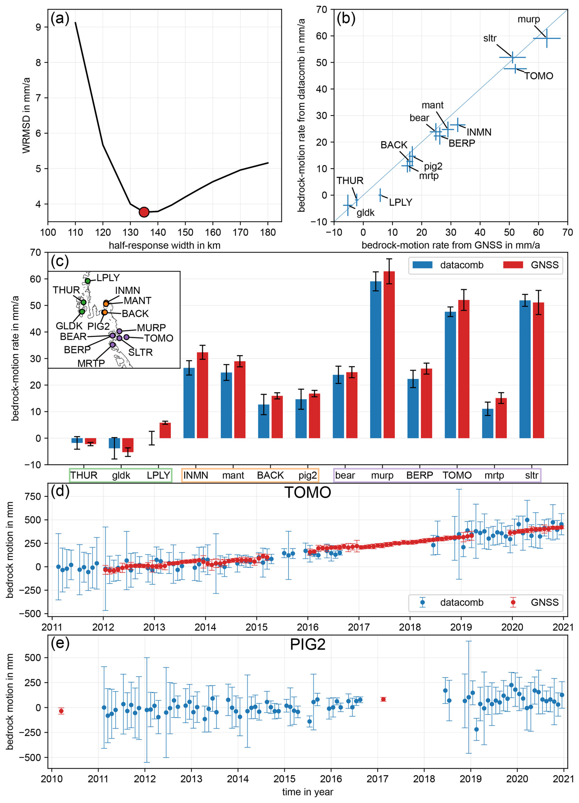
Figure 2 Comparison of bedrock motion from data combination (datacomb) and GNSS (GIA + elastic). (a) The weighted root mean square difference (WRMSD; Eq. 13) is a function of the Gaussian filter half-response width that we use to filter the input data. The combination results are evaluated at the GNSS sites. Applying a Gaussian filter with a 135 km half-response width (red circle) leads to a minimum WRMSD (optimal result). (b) A scatter plot of the optimal result showing bedrock motion rates from GNSS vs. data combination. Uppercase site names indicate that continuous data spanning more than 3 years are available. (c) Bedrock motion rates of the optimal result (blue) compared to GNSS-derived rates (red). The GNSS sites are categorized into three subregions: (1) peripheral glaciers (green), (2) Pine Island Glacier (orange), and (3) Thwaites Glacier (purple). (d, e) Bedrock motion from the data combination (blue) and GNSS (red) on the time series level for the GNSS station TOMO and PIG2 (Table 1), respectively. All uncertainties are 2σ.

Figure 3 illustrates maps of the mean rates of the determined GIA and IMC derived from the optimal result (cf. Fig. S4 for a cross section across the region highlighting the dominant signals). In the GIA field, we distinguish two local maxima around the Thwaites Glacier and the Pine Island Glacier. Additionally, Fig. S1 illustrates the two peaks in a cross-section plot. The determined GIA-related bedrock uplift rate peaks at 43 ± 7 mm a⁻¹ in the Thwaites Glacier region and at 32 ± 4 mm a⁻¹ in the Pine Island Glacier region. Near these maxima, minima are present at a distance of only ∼200 km (Fig. 3a), which is however close to the noise level. This transition from GIA-related uplift to subsidence is also visible in the GNSS data from Thurston Island (THUR and GLDK in Fig. 2c) and the Pine Island Glacier (INMN, MANT, BACK, and PIG2 in Fig. 2c).

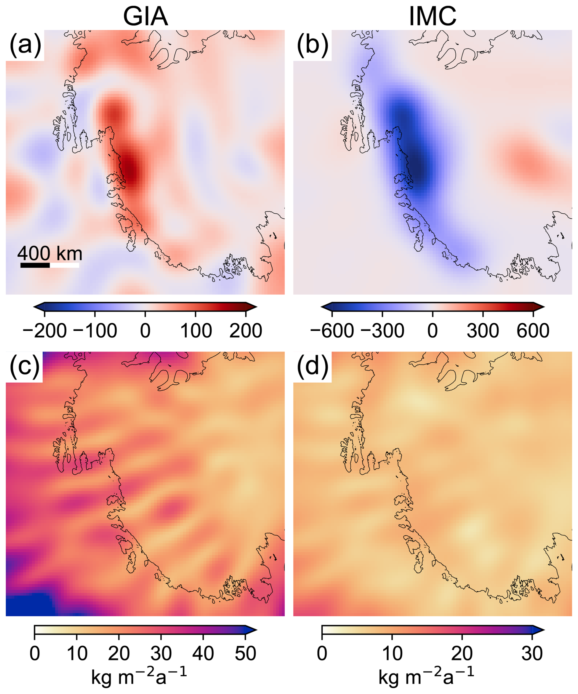
Figure 3 Maps of the results for (a) the GIA-induced surface density rate and (b) ice mass change as the surface density rate (i.e. equal to the rate of equivalent water height in mm a⁻¹). (c, d) Uncertainties obtained from Willen et al. (2022) propagated to GIA and IMC, respectively, on the trend level. Units are indicated in columns.

The combination method prescribes that the IMC and FAC results (Figs. 3b and S3) are as equally smooth as the resolved GIA. The sign of resolved IMC is opposite to the sign of GIA for large parts. The IMC integrated over basins 21 and 22 (as defined in Zwally et al., 2012, Fig. 1b) plus a 200 km buffer zone is −163 ± 7 Gt a⁻¹ for the time interval of January 2011 to December 2020. The apparent GIA mass effect integrated over the same region is +34 ± 3 Gt a⁻¹. The integrated FAC change over the same region is 14.6 ± 6.5 km³ a⁻¹. We use the 200 km buffer zone to account for signal leakage out of the integration area due to smoothing, but we neglect signal leakage into the integration area as this is expected to be minor (Gunter et al., 2014).

5 Discussion

5.1 Assessment and comparison

We find that the bedrock motion mean rates derived from the data combination based on GRACE/GRACE-FO and CryoSat-2 satellite data agree with those observed directly using GNSS within their respective uncertainties (Fig. 2c). Our spatially continuous inverse GIA estimate is the first to agree with vertical bedrock velocities from GNSS data in the ASE. Previous similar combination approaches (e.g. Gunter et al., 2014; Engels et al., 2018; Willen et al., 2024) have only been able to determine an overly smoothed estimate of the GIA uplift, thus only partly recovering the GNSS data in the ASE. These studies have found GIA-related vertical rates up to about 15 mm a⁻¹ in the ASE and a spatial pattern with long wavelengths and only one maximum, whereas GNSS observations suggest GIA-related vertical uplift of more than 40 mm a⁻¹ (Table 1). The restriction to long wavelengths also holds for the inverse approach of Martín-Español et al. (2016b), incorporating GNSS data in addition to gravimetry and altimetry data, as this study constrains the GIA parameterization to length scales of 500 km and larger. Even though the GIA parameterization is prescribed in such a way that shorter spatial scales are allowed in the ASE and the Antarctic Peninsula compared to the remainder of Antarctica, the length scale is still insufficient to resolve the spatial scales that GNSS data suggest. Although Martín-Español et al. (2016b) include GNSS observations in the estimation procedure, there are still large misfits between the GIA estimate and the GNSS data, in particular in the ASE. This remains the case for a modification of this approach in Martín-Español et al. (2016a) that allows for shorter spatial wavelengths in the ASE but which are presumably still overly large. Likewise, Sasgen et al. (2017) present GIA estimates at a spatial resolution of 200 km, based on an inversion that includes GNSS data, in addition to gravimetry and altimetry data. Even though they resolve GIA-related vertical uplift rates of close to 20 mm a⁻¹, these magnitudes and spatial scales of estimated GIA are still insufficient to explain the GNSS data.

In contrast to previous combination approaches and most GIA forward-modelling results (Whitehouse et al., 2019), we can resolve two distinct local maxima of the GIA-related bedrock motion in the ASE: namely in the area of the Pine Island Glacier and in the area of the Thwaites Glacier (Figs. 3a and S4). These two maxima are also postulated by the GIA forward-modelling approach of Barletta et al. (2018), which best fits GNSS observations (Fig. 4a and b) when using a low-viscosity upper mantle of 4×10¹⁸ Pa s and a centennial loading history in the ASE. Figures 4 and S5 illustrate the comparison of the GIA vertical motions that we obtain and the modelling result from Barletta et al. (2018). In the ASE, the results of both approaches provide a similar spatial pattern (smoothness and shape) and magnitude. The difference image (Fig. 4c) shows that the maxima of the Pine Island Glacier and Thwaites Glacier largely coincide. Nevertheless, there are significant deviations that can be attributed to limitations of the data combination method (noise in the GIA solution) as well as the modelling approach by Barletta et al. (2018) (strict focus on the ASE).

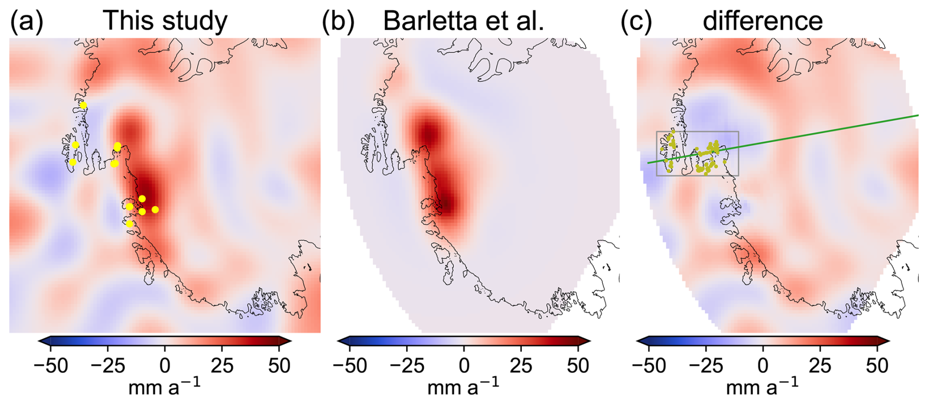
Figure 4 (a) The GIA result from the data combination expressed as the bedrock motion rate. Yellow dots mark positions of GNSS sites (Fig. 2c). (b) The GIA forward-modelling result from Barletta et al. (2018) with the best fit to the GNSS rates in this region. (c) The difference between (a) and (b). The grey box marks the region of sign reversal of bedrock motion that may be of interest for further investigation. The green line shows the 100° W meridian, and the olive dots are rock outcrops from Burton-Johnson et al. (2016) provided via Quantarctica3 (Matsuoka et al., 2021).

5.2 Spatial resolution

The spatially continuous GIA uplift rates from the data combination reveal spatial features at a scale of less than ≈200 km, visible in Fig. 3a. Our results indicate a sign reversal on short spatial scales that shows in the GNSS-derived rates too, e.g. by comparing the GIA-related rate at the THUR site at Thurston Island of −4.0 ± 0.6 mm a⁻¹ and at the INMN site close to the Pine Island Glacier of 23.6 ± 2.6 mm a⁻¹ (Table 1). We may interpret these as the resolved forebulge, but some part of these spatial features is likely related to Gibbs artefacts and could only be truly verified by further in situ measurements. A profile of several GNSS sites located approximately along the 100° W meridian from Thurston Island to the Pine Island Glacier would be very helpful to investigate the sign reversal of bedrock motion in more detail. This would be, however, also challenging due to the limited availability of bedrock outcrops (Fig. 4c).

We attribute our success in continuously spatially resolving the mass change signals at a realistic order of magnitude to the large signal-to-noise ratio in the ASE: both IMC and GIA signals are large. Moreover, the noise of GRACE/GRACE-FO data is comparatively low locally, as these missions have a polar orbit and the study area is located in a high-latitude region; i.e. the spatial sampling is higher than in areas of lower latitude (e.g. Yang et al., 2024). In other words, spherical harmonic coefficients of high degrees and low orders can be determined with more accuracy than coefficients of high degrees and high orders. The half wavelength of a field given as spherical harmonics is usually used to describe its spatial resolution (e.g. Vishwakarma et al., 2018). A rule of thumb is 20 000 km per L (maximum degree of development). It might be misleading to assess the spatial resolution of GRACE/GRACE-FO gravity fields on a grid in the spatial domain as the theoretical resolution differs in the longitude and latitude direction due to meridional convergence (e.g. Vishwakarma et al., 2018). Expressed in degrees instead of equatorial circumference, the theoretical resolution is 180° per L in the latitude, θ, direction and cos (θ)180° per L in the longitude direction. For L=96 this results in 1.875°; i.e. the theoretical resolution in latitude direction is $\mathrm{1.875}\times (\mathrm{40}\mathrm{000}\mathrm{km}/\mathrm{360}\mathit{°})\approx \mathrm{208}\mathrm{km}$. The latitude of our study region is $\mathit{\theta }=\sim \mathrm{75}$° S; hence in the longitude direction the resolution is $\cos (\sim \mathrm{75}\mathit{°})\times \mathrm{1.875}\mathit{°}\times (\mathrm{40}\mathrm{000}\mathrm{km}/\mathrm{360}\mathit{°})\approx \mathrm{54}\mathrm{km}$. This approximation holds for a sphere and is slightly different for an ellipsoid. Moreover, the spatial resolution is affected by the Gaussian smoothing applied on the polar stereographic grid in the spatial domain. The Gaussian smoother equally averages information in the longitude and latitude direction. The combined effect may be simply approximated by averaging with $(\mathrm{208}\mathrm{km}+\mathrm{54}\mathrm{km})/\mathrm{2}=\mathrm{131}\mathrm{km}$, which is actually close to the Gaussian smoother half-response width of 135 km that we find for our best-fit result.

The evaluation of gravitational fields on an ellipsoid using the method from Ditmar (2018) allows for a more realistic assessment of surface density changes. In particular in the ASE region, Ditmar (2018) showed that the evaluation on a sphere in contrast to an ellipsoid causes up to 15 % difference in the signal magnitude. A test run using a spherical approximation (Wahr et al., 1998) has shown that we need to choose a larger Gaussian filter (160 km half-response width) to achieve a best fit with the GNSS data. From this, we conclude that the ellipsoidal approximation allows for a higher spatial resolution than the spherical approximation in the combination approach, as the ellipsoidal surface allows for a more realistic assignment of the mass change signal.

5.3 Limitations

We find a bias of 0.9 mm a⁻¹ when comparing the GNSS uplift rates with the combination results (Sect. 4). We argue that due to the large GIA uplift of up to 43 ± 7 mm a⁻¹, errors of less than 1 mm a⁻¹ over a 10-year period are hardly relevant (Fig. 2c). Systematic errors responsible for the small bias may be long-term climate trends outside the modelling period of the utilized regional climate model (RACMO2.3p2: 1979–2021), which could cause a trend error (Medley and Thomas, 2019). Furthermore, the firn model needs to be initialized over a reference period to generate an equilibrium firn layer. We assume that there are no dominant climate trends over the reference period, which is 1979–2021 in the case of IMAU-FDM (Veldhuijsen et al., 2023). However, this assumption may not be valid in reality. If there are climate trends during the initialization, this assumption will lead to errors in the trend (Thomas et al., 2017). Even though we argue that the bias given by the signal-to-noise ratio is hardly relevant, this may not apply to other regions of Antarctica. We recommend a thorough error characterization of the input data when aiming to determine signals outside of the ASE region. This plays a crucial role especially for the evaluation of altimetry over the East Antarctic Ice Sheet where firn thickness variations dominate over changes in ice flow dynamics and assessing firn thickness variations remains a challenge (Kappelsberger et al., 2024). In addition, there are uncertainties in secular timescales of the GNSS solutions, which are induced by the realization of the terrestrial reference frame. For example, ITRF2014 shows a drift of 0.2 mm a⁻¹ in translation of the z coordinate compared to the current realization of ITRF2020 (Altamimi et al., 2023), which particularly maps onto the vertical velocities in polar regions.

Moreover, our estimation procedure does not take far-field effects and the error covariance structure of GRACE/GRACE-FO into account, as done in some other combination approaches (e.g. Willen et al., 2024), which potentially leads to errors in the result. However, we use the covariance information of the input datasets for estimating the uncertainties introduced by far-field signals. Willen et al. (2022) indicated that for the grounded AIS, far-field effects due to hydrological and glacier mass changes for a 10-year period are on the order of 1 and 10 Gt a⁻¹, respectively. If we assume the estimated GIA to fully absorb the far-field effects, this would result in a GIA bedrock motion bias of 0.02 and 0.2 mm a⁻¹, respectively (assuming an area of the grounded AIS of about 12×10¹² m², an effective GIA density of 3700 kg m⁻³, and a uniformly distributed far-field effect).

The assumptions about the effective densities (Eqs. 7 and 8, Fig. S2) in Eqs. (10) and (9) may also contribute to the bias. We base the relation between mass changes and volume changes in the various processes on previous studies (e.g. Riva et al., 2009; Gunter et al., 2014). Investigations with GIA models and ice sheet models may reveal whether further improvements in the estimation can be achieved by refining these effective densities.

As mentioned in Sect. 3, there is an inconsistency in the applied methodology when taking into account elastic deformations that occur due to contemporary changes in ice mass (i.e. changes in uplift). We quantify this inconsistency (Sect. S1) and find it is negligibly small.

We use the data at a monthly resolution, as these are available at this temporal resolution. However, we refrain from drawing conclusions about temporal variability in the bedrock motion rates based on our results at the time series level (Fig. 2d, e), as the estimates are too noisy and large uncertainties are present. This may also hold for GNSS time series (Koulali and Clarke, 2020). At the TOMO station (Fig. 2d), temporal fluctuations are caused in particular by error effects such as accumulated ice in the antennas or equipment changes. Since 2017, such error effects have been eliminated, e.g. by sealing the antenna. Future studies may investigate whether it is possible to manage these errors and to derive time-variable rates related to transient solid-Earth deformation (Simon et al., 2022). Based on findings from Powell et al. (2020), we do not expect that significant rate changes related to viscous deformation caused by recent IMC are detectable over an investigation period of only 10 years. When assuming low upper-mantle viscosity, significant viscous effects should only be measurable from ≈20 years onwards.

5.4 Outlook

The estimated GIA-related bedrock motion is an excellent dataset for validating GIA models and coupled GIA–ice sheet models (van Calcar et al., 2023; Albrecht et al., 2024). In contrast to GIA-induced vertical bedrock motion rates from GNSS, the data-combination-based result spatially continuously provides information on GIA in the ASE region, even where the bedrock is covered with ice. Assumptions on a locally adapted, 3D, or transient rheology in this region, as well as assumptions on the ice-loading history, may be verified with the present-day GIA effect determined here.

A monthly temporal resolution is certainly not necessary to determine GIA on the time series level, as we do not expect GIA to fluctuate on these short timescales. Nevertheless, temporal variations in GIA rates due to effects related e.g. to transient rheology are an evolving subject of investigation. GIA modelling based on transient rheology can be helpful to find a temporally reasonable parameterization that ranges between a monthly and constant rate for future studies.

In other regions of Antarctica, the signal-to-noise ratio is much smaller so that a more extensive error analysis (e.g. Willen et al., 2024) is required to retrieve sound results. Future satellite gravimetry missions (Daras et al., 2024) and evaluation of time-variable gravity data on the trend level (Loomis et al., 2021; Kvas et al., 2023) might be useful for assessing mass changes in the ASE and other regions at an even higher spatial resolution. This may allow us to further decrease the spatial smoothing applied to the input datasets and could resolve smaller-scale GIA patterns if they exist. High-quality GNSS data with a favourable spatial coverage would be necessary to validate such investigations.

In this study, we distinguish between an elastic response and GIA as two separate deformation effects. Particularly in the ASE region, this distinction will not be possible for investigation periods of several decades, as these effects overlap over multi-decadal periods in this region (Powell et al., 2020). In the future, the longer observation time series of 20 years and more will become increasingly relevant to investigating whether we can quantify the viscoelastic deformation effects of the solid Earth that were triggered by the loading changes during satellite observations and viscoelastic deformation in response to ice-loading changes on centennial and millennial timescales.

6 Conclusions

This study presents a regional combination method using data from GRACE/GRACE-FO, CryoSat-2, regional climate modelling, and firn modelling. For the first time, this combination of data resolves vertical bedrock motion rates in the Amundsen Sea Embayment that agrees with rates from GNSS on bedrock. We resolved a GIA-induced uplift of more than 40 mm a⁻¹ at maximum, whereas previous data combination approaches have only resolved less than half of this magnitude at maximum. The results reveal that GIA masks about a quarter of the total observed mass loss in this region from January 2011 to December 2020. We assign −163 ± 7 Gt a⁻¹ to the ice mass change and +34 ± 3 Gt a⁻¹ to the apparent mass effect caused by GIA. Thus, we determine present-day GIA effects in a region where it is a great challenge to forward-model GIA, as both the rheology and the decisive centennial ice-loading history come with significant unknowns (Whitehouse et al., 2019). The large signal-to-noise ratio in this area permits some error contributions to be ignored so that agreement with GNSS within the errors is still guaranteed. The resulting GIA estimates may be particularly useful for coupled ice sheet–solid-Earth models (van Calcar et al., 2023; Albrecht et al., 2024) to study the feedback between bedrock motion and glacier flow, which may foster improvements of feedback predictions. So far, our approach has justified resolving long-term (>10-year) temporal variations in bedrock motion rates only, as short-term variations are dominated by short-term errors in the input data.