Review article: Feature tracing in radio-echo sounding products of terrestrial ice sheets and planetary bodies

This paper aims to inform researchers and practitioners in radioglaciology about current and future trends in mapping the englacial stratigraphy of ice sheets. Radio-echo sounding (RES) is a useful technique for measuring the subsurface properties of ice sheets and glaciers. One of the most important and unique outcomes is the mapping of ice sheets' englacial layer stratigraphy, mainly consisting of isochronous reflection horizons. Mapping those is still a labor-intensive task. This review provides an overview of state-of-the-art (semi-)automated methods for identifying ice surface, basal, and internal reflection horizons from radargrams in radioglaciology. Methods for segmenting (and detecting) different regions of radargrams are also included due to their data and methodological similarity to methods tracing internal reflection horizons. We discuss a variety of methods which have been developed or applied to RES data over the last few decades, including image processing, statistical techniques, and deep learning approaches. For each approach, we briefly summarize their procedures, challenges, and potential applications. Despite major advances, we conclude that gaps remain in effectively mapping internal reflection horizons in an automated way but with deep learning representing a potential advancement.

1 Introduction

Radio-echo sounding (RES) is a powerful technique which has been used in radioglaciology for more than 50 years to investigate subsurface properties of polar ice sheets (Schroeder et al., 2020). It has proven useful for determining widespread basal topography and ice thickness on glaciers as well as in inaccessible regions such as the Antarctic and Greenland ice sheets. Historically, RES systems applied in glaciology have also been referred to as ice-penetrating radar (IPR). For ground-based applications, ground-penetrating radar (GPR) is used as well (Bogorodsky et al., 1985). To refer to the most general meaning, we will follow the recommendations of Schlegel et al. (2022) for terminology and only use radar or RES, unless more specific terms are necessary in the context. RES data not only reveal information about the base of the sheet and ice thickness, but also provide insights into its internal structure. Such insights are obtained from the presence of englacial reflections and backscatter characteristics in RES data, most prominently internal reflection horizons (IRHs), also known as internal radar reflections (Schlegel et al., 2022). These IRHs are a result of variations in the dielectric properties of the ice, which can be attributed to changes in density, impurity content, acidity, or crystal orientation fabric (Moore and Paren, 1987; Eisen et al., 2007).

It has been shown that IRHs, caused by changes in conductivity, are generally isochronous – i.e., one horizon has the same age everywhere (Gudmandsen, 1975; Siegert, 1999; Fujita et al., 1999; Eisen et al., 2006) – serving as indicators for paleoglaciology (Siegert, 1999; Fahnestock et al., 2001; Miners, 2002; Jansen et al., 2024). Englacial horizons observed in RES datasets have also been utilized to investigate ice dynamics, calibrate ice-flow models, estimate past accumulation rates, and constrain layer ages from ice cores (Siegert et al., 2004; Rippin et al., 2006; Conway et al., 1999; Waddington et al., 2007; Schroeder et al., 2020; Sutter et al., 2021). Geometry of isochronal radar reflection horizons, in conjunction with ice-flow modeling, can provide significant perspectives into ice dynamics, basal sliding, surface accumulation history, and englacial folding (Waddington et al., 2007; Nereson and Raymond, 2001; Hindmarsh et al., 2009; Catania and Neumann, 2010; Leysinger Vieli et al., 2011; Lenaerts et al., 2014; Jenkins et al., 2016; Holschuh et al., 2017; Born and Robinson, 2021; Bons et al., 2016; Sutter et al., 2021; Jouvet et al., 2020; Jansen et al., 2016). Additionally, stratigraphic information provided by englacial layers complement ice-core analyses, improving interpretation of climate changes recorded in ice cores by revealing flow paths and irregularities that may affect age stratigraphy at ice-core sites (Fahnestock et al., 2001; NEEM community members, 2013; Parrenin, 2004). To support joint international and collaborative exploitation of the available radar datasets, the Scientific Committee on Antarctic Research (SCAR) has endorsed the AntArchitecture Action Group, specifically dedicated to cataloging IRHs across the entire Antarctic ice sheet (Bingham et al., 2024).

One of the earliest publications on internal reflections by Bailey et al. (1964) details the observation of a continuous echo at the depth of 500 m as well as a 97 % continuous basal layer after a series of measurement campaigns in Greenland. They noted that compacted annual accumulation is the cause of such echoes (reflections). Moreover, other early works such as works of Gudmandsen (1975) and Robin (1975) exclusively discuss RES measurements over ice sheets and their interpretations (Paren and Robin, 1975; Clough, 1977). IRHs are traditionally identified by manually or semi-automatically tracing individual reflections within RES datasets, a laborious and time-consuming process (Nereson et al., 2000; Waddington et al., 2007). It has been shown that tracing 20 IRHs in 20 000 km of data in such a way would take 10 operator years to complete (Sime et al., 2011). To overcome the slowness of manual tracing, since the 1980s, some commercial software programs have been used for semi-automated mapping of IRHs. Some other programs have been complemented by open-source software modules provided by the community, in addition to processing and analyzing RES data. Some examples include software packages such as MATLAB (MathWorks, 2022); toolboxes such as GPRlab (Xiong et al., 2024), GSSI Radan (GSSI, 2024), ReflexW (Sandmeier, 2016), the Sensors & Software EKKO Project (Sensors Software Inc, 2024), and Geolitix (Inc., 2025); and open-source software packages such as the ImpDAR (Lilien et al., 2020) library for Python and RGPR package (Huber and Hans, 2018) for R.

The age stratigraphy obtained from the Antarctic ice sheet, unlike the Greenland ice sheet (MacGregor et al., 2015), has been limited to specific regions (MacGregor et al., 2015; Siegert et al., 1998; Eisen et al., 2004; Siegert et al., 2004; Steinhage et al., 2001; Leysinger Vieli et al., 2011; Cavitte et al., 2016; Winter et al., 2019), resulting in an incomplete picture of its englacial architecture. Several challenges slow down the achievement of a continent-wide stratigraphy. The considerable time required for tracing IRHs, limited spatial coverage of available data, and a lack of integration between stratigraphic information from different RES systems (Cavitte et al., 2016; Winter et al., 2017) are among these challenges. However, the primary challenge remains to be the imbalance between the number of available data and the amount of time required with available methods to map the stratigraphy. In terms of size, the Antarctic ice sheet surpasses the Greenland ice sheet more than 6-fold. While most of the Greenland data have already been analyzed for internal stratigraphy, there still exists a significantly larger volume of unexplored data from Antarctica compared to that of Greenland. In addition, there are still some areas of the Antarctic ice sheet over which RES surveys have not been performed (Frémand et al., 2023).

This limited advancement of methodologies for assessing the structural configuration of the stratigraphy across large spatial scales challenges exploration of englacial architecture of the Antarctic ice sheet (Delf et al., 2020). To overcome the difficulties associated with manual picking of IRHs, there has been a growing interest in developing (semi-)automatic methods for tracing IRHs in RES echograms (also known as “radargrams”, as well as B-scans; Jol, 2009), in particular from airborne operations. The motivation behind these efforts is to reduce the amount of human labor required for data analysis, particularly as radar datasets have expanded over large spatial scales (Medley et al., 2014; MacGregor et al., 2015; Cavitte et al., 2016; Koenig et al., 2016; Delf et al., 2020), as well as reduce subjectivity of interpretations of IRHs (Dossi et al., 2015). Automated horizon-picking techniques have shown some potential, but they still require some operator input and are yet to effectively map IRHs.

In the past 2 decades, there have been various research attempts by several research groups at automatically tracing ice–bed boundaries, mapping reflections, tracing firn-layer boundaries, and segmenting regions of radargrams from both ice sheets and planetary radargrams. Yet, a complete account of this long-lasting endeavor which contains a comprehensive overview of all the methods – and regions these methods were applied to – has been missing.

In this review paper, we present an overview of the available methods for tracing layer boundaries and IRHs in radargrams. By presenting various studies and approaches, we aim to provide insights into advancements, challenges, and future directions. In Sect. 2, we briefly discuss the RES technology and the terminology that is necessary for understanding radar products. Section 3 introduces the methods that have been employed by various research groups in a timeline of method development for the task of stratigraphy mapping. A comprehensive timeline of the published works with a short summary of each publication, remarking on the more relevant information of each of the publications, is discussed in Sect. 4. Finally, we provide a discussion and a conclusion and outlook in Sects. 5 and 6, respectively, highlighting the need for automatic methods to fully exploit the extensive datasets and labor-intensive nature of manual picking and analyzing recent trends with potential directions of future research.

2 Background

In this section, we provide the necessary concepts and information related to RES. We start with introducing radioglaciology and go on to describe radargrams and IRH representations. For further details on radar physics and applications, we refer the reader to the available radar literature (Bogorodsky et al., 1985; Plewes and Hubbard, 2001b; Dowdeswell et al., 2008; Bingham and Siegert, 2007; Pellikka and Rees, 2010; Woodward and Burke, 2007; Daniels, 2004).

2.1 Radioglaciology

Radioglaciology is the scientific field that employs radar (radio detection and ranging) systems to explore the cryosphere, including both satellite and airborne as well as ground-based systems. RES is an active remote sensing method which, unlike satellite imagery, can give a picture of the cross section of an ice sheet. An electromagnetic waveform is emitted from a transmitter antenna, penetrates the ice, and is reflected by changes in the complex-valued permittivity of ice. The reflection travels back to a receiving antenna. Reflective properties are influenced by various factors such as density (presence of bubbles), the orientation of ice crystals, inhomogeneities, impurities, and the geometry of the materials. Applications range from determining ice thickness; identifying englacial and subglacial properties, e.g., lakes; reconstructing past ice-dynamic changes; and extrapolating ice-core records. Related studies have employed airborne, ground-based, or orbital RES systems on terrestrial and planetary ice bodies. In the following, we will give a brief account of RES physics and applications but refer the reader to the available publications previously mentioned for further details.

For our objective in this review, the important information derived from radargrams is the englacial layer architecture. Such layer boundaries, known as IRHs, were formed at the former ice sheet surface, then advected into the ice by additional accumulation and deformed by ice flow. At different depths of the ice sheets, various processes can change the complex-valued permittivity, causing IRHs. IRHs primarily originate from density fluctuations in the upper part and variations in dielectric conductivity (e.g., from acidity; MacGregor et al., 2012) in deeper regions of the ice sheet. In the middle to deepest layers of the ice sheet, changes in the crystal orientation fabric can also result in reflections (Fujita et al., 1999; Eisen et al., 2007).

2.2 Radar products

In radioglaciology applications, out of every single survey line, a 2D cross-sectional profile of the ice sheet is produced. This product is called a radargram or an echogram. In older texts, as well as some contemporary publications, similar profiles were called Z-scope records (Schroeder et al., 2022). A radargram depicts a full profile of the cross section of the ice sheet as opposed to single traces. It is usually composed of single transmit signals and reflections. In the case of single-point measurements, they are stored as amplitude displays which are also called A-scopes (also referred to as A-scans) and are similar to panels (a) and (b) of Fig. 1. When reflections are laterally coherent, they appear as continuous horizons. Every pixel within the radargram corresponds to the quantification of amplitude (or power) associated with the radar wave that is reflected by subsurface interfaces positioned at a designated range (two-way travel time or depth) location and a spatial coordinate within the azimuthal direction.

Figure 1 depicts different representations of a trace and a vertical section of the same profile. Panels (a) and (b) represent an arbitrary trace with a 60 and 600 ns pulse, respectively. Panels (c) and (d) show a section of a radargram with the leftmost trace shown in panels (a) and (b), and panels (e) and (f) show the same radargram sections composed of differentiated traces. In most cases for older systems, where the phase was lost because of rectification of the received signal, studies are done using the differentiated radargrams as they illustrate a clearer picture of the englacial architecture. In this figure, the ice surface (air–ice interface), base (ice–base interface), englacial reflection, and so-called echo-free zone (EFZ, just above the bed) can be seen. The EFZ in the conventional sense was affected by different factors, e.g., system sensitivity or a lack of coherent reflections owing to disturbances possibly from ice flow near the interface of ice and the base (Drews et al., 2009).

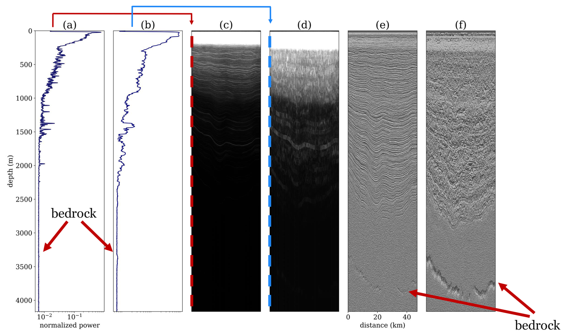
Figure 1 An example of a vertical section of a radargram and a single trace from it. The section is from a flight performed in 1999 between Dome Fuji and Kohnen station (Steinhage et al., 2013): (a) trace (A-scope) with 60 ns pulse; (b) trace (A-scope) with 600 ns pulse; (c) vertical section of raw radargram (Z-scope) with 60 ns pulse; (d) vertical section of raw radargram (Z-scope) with 600 ns pulses; (e) vertical section of differentiated radargram (Z-scope) of panel (c); (f) vertical section of differentiated radargram (Z-scope) of panel (d). Panels (c), (d), (e), and (f) show the same section.

Individual measurements are often noisy, typically due to the electromagnetic interference from other electronics, such as aircraft and other components in the vicinity of the instrument, as well as thermal noise. Therefore, radar traces are usually stacked to increase the signal-to-noise ratio and obtain enhanced subsurface images (Karlsson et al., 2012). In the presented Fig. 1, each plotted trace is a stack of 10 consecutive traces.

2.3 Internal reflection horizons

In the radargram of Fig. 1, reflection signatures can be seen in different regions such as close to the surface, englacially, and subglacially. The most general term to refer to any signal in the data which is not noise is event. Such events are illustrated in Fig. 2, which is a simplified schematic of a radargram, where differences between ice layers and IRHs are depicted. The ice surface at the top (blue line) and basal reflection (black line) at the bottom of the ice are also shown. The first reflection of each transmitted pulse of an airborne survey is the reflection from the ice surface.

For the sake of facilitating analyses of radargrams, one of the common practices is to synchronize all traces to time zero at the air–ice interface, omitting topographical variations. This flat ice surface naturally appears in ground-based systems; however, for airborne systems, this assigning of the surface time as zero is a step during data processing. The black line depicts the basal reflection. The red lines in the radargram indicate IRHs. In an ice sheet, these represent the interfaces between the neighboring ice layers of different dielectric properties.

2.4 Applications of englacial stratigraphy in glaciological research

Englacial stratigraphies deduced from RES data are increasingly used to benchmark and validate ice-dynamic models (Sutter et al., 2021; Björnsson and Pálsson, 2020; Bingham et al., 2024). Several englacial features can be seen in radargrams, which can be studied in both quantitative and qualitative ways (Plewes and Hubbard, 2001a; Pellikka and Rees, 2010). Quantitative studies take advantage of the amplitude and phase of traces and are often used to derive physical properties of ice (Plewes and Hubbard, 2001b). Qualitative studies, in contrast, mostly utilize stratigraphy to infer the current of past flow dynamics or boundary conditions, e.g., surface accumulation (Arcone et al., 2005) or basal melting (Bogorodsky et al., 1985). Some of the many applications of englacial stratigraphy are to study past ice stream dynamics (Keisling et al., 2014; Winter et al., 2015; Jansen et al., 2024; Carter et al., 2023), glacier–volcano interactions (Björnsson and Einarsson, 1990), meltwater drainage (Pitcher et al., 2020), glacier hydrology and dynamics (Eisen et al., 2020), glacier response to climate shifts (Guðmundsson et al., 2009), mass balance (Kowalewski et al., 2021), glacier evolution (Aðalgeirsdóttir et al., 2011), and volcanic activities (Brandt et al., 2005b). RES is also used to identify subglacial properties, such as lakes (Bowling et al., 2019), which appear as strong and rather flat features at the bottom of the ice, owing to the high permittivity of liquid water in contrast with the overlaying ice.

For a variety of applications such as developing compilations of bedrock topography (Lythe and Vaughan, 2001; Frémand et al., 2023), synchronizing ice cores (Steinhage et al., 2013; Cavitte et al., 2016), paleoglaciological studies (Parrenin et al., 2017), ice dynamics (Jansen et al., 2024), mass balance derivation (Brandt et al., 2005a), and ice sheet modeling (Sutter et al., 2021), the key is to have a mapped englacial stratigraphy or mapped basal surface. In the next section, we look into the most common methods that have been used to map englacial stratigraphy.

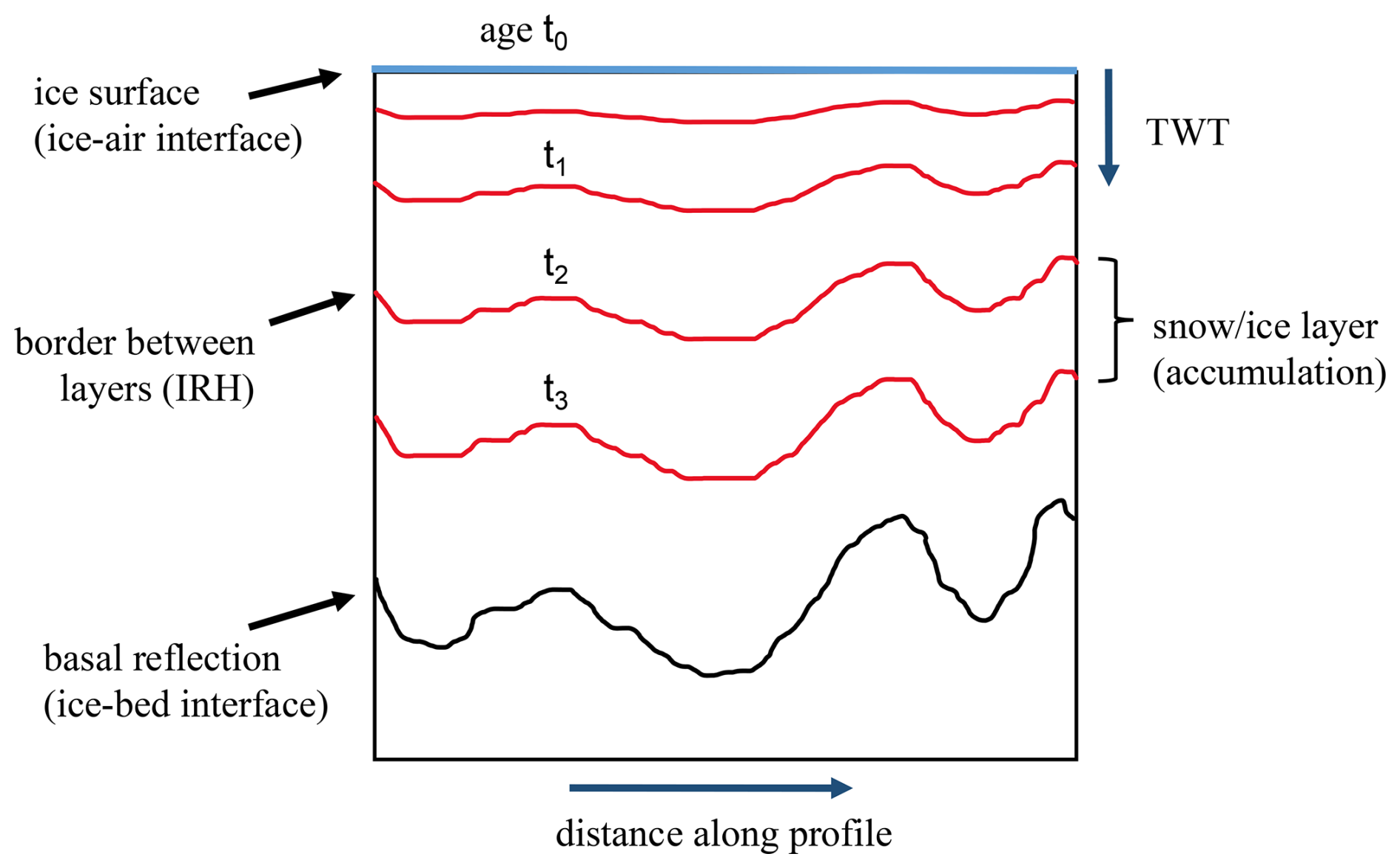
Figure 2 Schematic of a radargram. The blue line at the top represents the surface of the ice sheet (ice–air boundary). It is conventionally set as time zero discarding topography. The red lines are IRHs which represent the changes in the permittivity that could be present on the boundaries between different layers. The black line at the bottom is a representation of the ice base. The x axis is the distance in the direction of the flight, and the y axis can be shown as either two-way travel time (TWT) or depth.

3 Overview of applied methods

In this section, we provide a brief overview of the methods that have been applied to tracing IRH and segmenting radargrams for identification of different classes or targets. The subsections related to each method provide information on how the respective method has been used for this task. We present more details on implementation in the timeline of publications in Sect. 4.

Given the versatile applications of RES across various domains (as mentioned in Sect. 2.4), efforts to characterize features within radargrams or to map reflections have proven valuable across various fields, including contamination assessment, hydrology, archaeology, geotechnical engineering, and glaciology (Jol, 2009).

Based on a number of studies, it seems that constructing an automated tracing method for RES encounters a significant challenge when dealing with closely spaced layers. This situation gives rise to numerous horizon candidates that are nearly identical but slightly offset from each other. If the algorithm mistakenly selects the wrong candidate, it may veer into adjacent horizons, leading to inaccurate tracing (Panton, 2014). This situation is more relevant when regarding deep IRHs. The IRHs in snow and firn radargrams have much less compaction as well as vertical fluctuation (Winter et al., 2019). This is the primary reason why automatically identifying and differentiating deep englacial horizons is much more challenging than detecting near-surface and basal reflections.

The methods to map the near-surface, basal, or englacial architecture of the ice can be categorized on the basis of a variety of criteria. One such criterion is if a method operates semi-automatically or fully automatically. By semi-automatic, we refer to methods that require manual tweaking, interference, or initialization by a user. Another category is if the proposed method does or does not include machine learning algorithms. It is also possible to categorize methods based on the depth or specific reflection that they are designed for. Some methods (mostly earlier ones) are only aimed at tracing surface and basal reflections in order to estimate ice thickness; others look into englacial events.

The complexity of tracing englacial layers is caused by

• the limitation of vertical resolution (e.g., two IRHs merging into one);

• the limitation of horizontal resolution (e.g., steep IRHs leading to spatial aliasing);

• a small signal-to-noise ratio;

• a lack of discrete boundaries between layers;

• complex englacial structures, e.g., folds and interrupted horizons.

We will give a short summary of the methods that have been utilized in mapping and segmenting radargrams. The summaries of methods provided are intended to give a first overview and to later aid the understanding of the methodological evolution presented in Sect. 4.

3.1 Cross-correlation and peak following

Cross-correlation identifies similarities between two signals. Peak following typically refers to a control strategy used in systems where one variable is controlled to follow the peaks or high points of another (Fahnestock et al., 2001). This method is sensitive to noise and is prone to tracing discontinuous IRHs. Stratigraphy mapping, cross-correlation, and peak following enforce and complement each other in a manner whereby first a peak is calculated within a certain vertical window, which is the strongest return in the case of radargrams. Next, the cross-correlation is used to find a similar pattern in the radargram. Depending on the backscatter characteristics and spatial coherence, each method performs more efficiently in different areas of a single radargram (Fahnestock et al., 2001). This method has its roots in seismic applications, which have often been used for data processing and analysis in glaciology (Eisen et al., 2004, 2006). The assumption of this method is that ice stratigraphy is supposed to be rather smooth and without steep variations.

3.2 Edge detection and thresholding

An edge in an image is considered to be the location of abrupt change in pixel intensity. One of the most prominent filters used in edge detection is the Canny operator (Canny, 1986). It is a special filter kernel that is convolved with the image, smoothes the image to remove some noise, and simultaneously calculates the gradient of the image to determine locations with high spatial derivatives. The next step is to follow along the gradient and suppress pixels that are not maxima, a process called non-maxima suppression. Lastly, it is necessary to apply thresholding and remove weak edge pixels. Having been in use for more than 3 decades, the Canny edge detector is still widely used and efficient in detecting edges in a number of applications, e.g., to capture sharp breaks or discontinuities in an image (Canny, 1986). Speckle noise, which appears as a grainy pattern in radargrams, can create difficulties for the Canny filter. This noise often shows up as sudden changes in pixel intensity, which the gradient calculation in the Canny filter might mistake for edges. To reduce the effect of speckle, applying a pre-filtering step, such as a Gaussian or median filter, before performing edge detection could be a solution. Thresholding is a simple process for segmentation as well. A brightness leap between an object or edge and background can be determined to differentiate objects and the background (Sonka et al., 2015). As a simple and computationally inexpensive method, it has been widely used in simple applications. However, more nuanced sorts of thresholding can be adaptive thresholding, p-tile thresholding, histogram-based thresholding, entropy-based thresholding, and so on (Sankur, 2004). Based on these properties image processing is expected to be an efficient method in tracing englacial horizons and has been applied to near-surface reflections (e.g., Freeman et al., 2010). However, it has been concluded that this detector works well only for the detection of surfaces due to presence of noise in radar and closeness and weakness of horizon boundaries (Mitchell et al., 2013a).

3.3 Active contour

3.3.1 Snake

A well-known computer vision method of active contours is the Snake (Kass et al., 1988). It consists of splines that are forced by external constraints and influenced by pixel intensity. In the context of active contours, a spline is a mathematical curve that is used to represent the contour or shape of an object or region of interest in an image. From there, two constraints are to be satisfied. One is for the spline to align with the high-gradient energy pixels, and the other is avoidance of having discontinuities between splines. An energy function is defined, and the cost of the first spline is calculated. Then the energy function is minimized to find the most optimum location in relation to the two constraints (Kass et al., 1988). In radargram applications, an active contour comprising a single particle per column is initially positioned at the uppermost portion of the radargram and subsequently sinks down until it reaches the designated horizon. The contour attains a convergence of optimization through the interplay of three distinct “forces”: (1) a gravity-like force exerted to propel the contour in a downward direction; (2) an upward force influenced by image edges, akin to buoyancy; and (3) a tension force operating between adjacent particles (Reid et al., 2010; Gifford et al., 2010). Active contour models have the advantage that they do not require radargrams with manually traced IRHs. The main disadvantage is that a Snake model is not able to maintain the complex topology of the evolving curve (Rahnemoonfar et al., 2017a). In terms of the automatization level, on the grounds of the initial seeding and curve placement, they are mostly considered semi-automatic methods. Figure 3 depicts the stages of the active contour, from the initial contour to the final one reaching the edge boundary. The arrays in the figure are some of the forces applied to the contour at each stage.

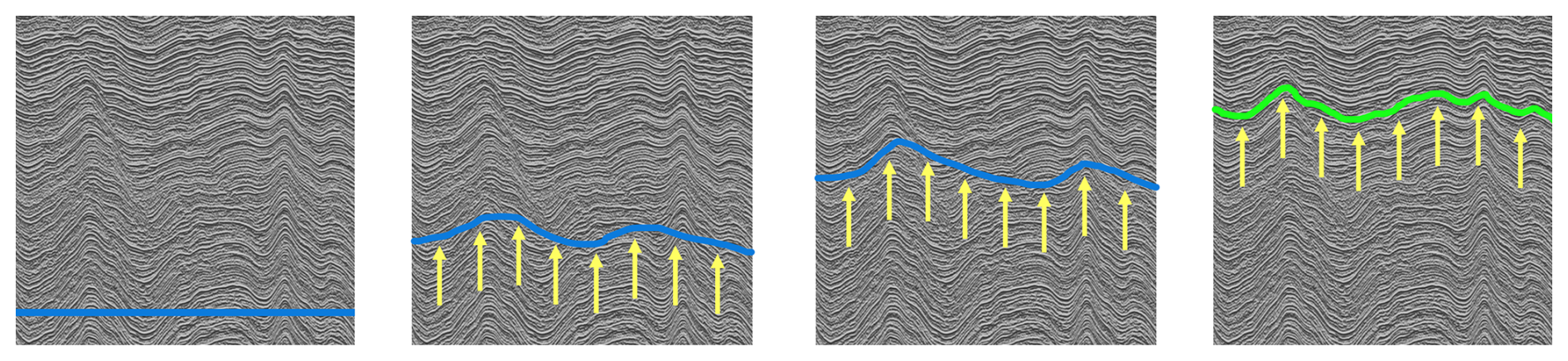
Figure 3 Application of a Snake or active contour method; the series from left to right shows the evolution of the initial contour until it reaches the boundary.

3.3.2 Level set function

This approach uses level set functions (LSFs) and presents a significant advancement in boundary delineation and image contours (Osher and Sethian, 1988; Malladi et al., 1995). It is a scalar field that signifies the signed distance to the nearest edge or boundary (Joshi et al., 2019). Distinguished from conventional Snake active contour model, the level set framework can work as well with no explicit initial contour parameterization (Lin et al., 2004), making it well-suited for the intricate analysis of radargrams. Optimizing a level set involves creating an energy or cost function, which governs the iterative minimization of the function to detect the object boundaries, using image attributes such as gradients and curvatures (Chan and Vese, 2001). The evolution of the initial curve is determined by a speed function, which in turn depends on factors such as image gradient, and involves a halting criterion which reduces the speed function to zero in high gradients delineating boundaries (Lin et al., 2004). The level set method has also proven efficient in other domains such as semi-automatic image segmentation for medical imagery (Lin et al., 2004; Chunming Li et al., 2011).

3.4 Statistical analysis

This method has been employed mostly for the characterization of subsurface target classes (Ferro and Bruzzone, 2012; Ilisei and Bruzzone, 2014, 2015). Its backbone is statistical analysis of the distribution of the radar signals. This is obtained by fitting several probability distribution functions (pdf's) to the histogram of samples from each target class in the radargram. The pdf's used to fit the signals are parametric models such as Rayleigh and Nakagami distributions (Ferro and Bruzzone, 2012; Ilisei and Bruzzone, 2014, 2015). The choice of such parametric models for the fits results from their proven capability to model radar amplitude fluctuations in signal backscatter (Oliver and Quegan, 2004).

3.5 Layer slope inference

Layer slope inference is not in fact a method but a combination of methods to calculate the dip angles of the horizons. It consists of the following: denoising using averaging techniques, thresholding to obtain the binary image from a radargram, discretizing the data horizontally to detect short segments of boundaries, eliminating the invalid objects, and finally compiling the non-uniformly distributed information on object dip (Sime et al., 2011). This method is rather easy to implement, but it does not map IRHs. Instead, it yields estimates of the potential layer boundaries and their dips and slopes (Sime et al., 2011; Holschuh et al., 2017).

3.6 Hough and Radon transforms

Hough (Hough, 1962) and Radon transforms (Radon, 1917) are very closely related to each other (van Ginkel and van Vliet, 2004). Radon (1917) introduced a method to express a function on the basis of its (integral) projections, and Radon transform is the mapping of this function onto its projection. As it maps from image space to parameter space, the function that is formed in the parameter space includes peaks which correspond to shapes or edges in the image space (van Ginkel and van Vliet, 2004; Radon, 1986; Epstein, 2007). The Hough transform is similarly mapping from image space to parameter space. In principle, the Hough transform is a discrete version of the Radon transform. It was originally developed to detect straight lines in black and white images (Hough, 1962). An accumulator array is set up, with each of its elements representing the number of votes that indicate the presence of a shape or edge with corresponding parameters of that element, signifying strong evidence for the existence of that line or edge (Duda and Hart, 1972; Bailey et al., 2020).

3.7 Continuous wavelet transform

Unlike traditional methods such as gradient-based edge detection (e.g., Sobel; Sobel and Feldman, 2015, Roberts Roberts, 1963), which rely on discrete derivatives, continuous wavelet transform (CWT) operates by analyzing the image at multiple scales and positions simultaneously (Mallat and Hwang, 1992). Considering all the values of the translation and scale parameters is the point where CWT differs from discrete wavelet transform, making it a preferred method for detecting specific features in images (Antoine et al., 1993). Mallat and Hwang (1992) established edge detection in a multi-scale method using wavelet transform. Locating an edge involves initially identifying the scale where the power spectrum, derived from the wavelet transform, reaches its peak. At this scale, the position of the peak in the squared CWT can be identified. CWT's advantages include multi-scale analysis for edge detection at various levels of detail and handling non-stationary signals, making it effective for complex image analysis (Mallat and Hwang, 1992; Kaspersen et al., 2001; Heric and Zazula, 2007). Another advantage is that CWT-based methods do not necessarily require thresholding, which reduces the complexity of an algorithm (Kaspersen et al., 2001).

3.8 Hidden Markov model and Viterbi algorithm

The application of hidden Markov models (HMMs) in the context of edge detection is an approach rooted in probabilistic modeling (Ekisheva and Borodovsky, 2006). HMMs, well-known for their efficiency in capturing sequential patterns, offer a great framework for identifying edges in complex and noisy radargrams (Carrer and Bruzzone, 2017; Donini et al., 2022b). They are based on augmenting the Markov chains which describes the probabilities of sequences of random variables to compute probabilities of observable events. In the case of radargrams, the observable events are pixel intensities. For edge detection, pixels within a radargram are conceptualized as hidden states, each one associated with emission probabilities indicating local intensity gradients. Transition probabilities, inferred from the gradients of neighboring pixels, represent the likelihood of going from one pixel to another, capturing the contextually dependent edge characteristics. By optimizing the sequence of hidden states, HMMs effectively capture IRHs in radargrams (Stauffer and Grimson, 1999; Ekisheva and Borodovsky, 2006; Zhang et al., 2008; Bouguila et al., 2022; Carrer and Bruzzone, 2017).

For any task containing hidden variables, it is important to find which sequence of such hidden variables is the underlying source of the desired observation. This is called decoding. One common such algorithm used along with HMMs is the Viterbi algorithm (VA; Viterbi, 1967), a dynamic programming technique, which finds the most plausible sequence of concealed states within a Markov field, depending on a series of observations (Bouguila et al., 2022).

3.9 Gibbs sampling

The Gibbs sampler (Casella and George, 1992) is a Markov chain Monte Carlo (MCMC) method for indirectly generating random variables from a (marginal) distribution, removing the need to directly calculate the density. Every pixel or region within the image is allocated a label representing its class or segment. Through iterative sampling of labels, considering conditional probabilities in neighboring pixels or regions, Gibbs sampling facilitates the partitioning of the image into coherent segments (Casella and George, 1992; Xiao Wang and Han Wang, 2004).

3.10 Support vector machine

The support vector machine (SVM) (Vapnik et al., 1996) is a supervised learning approach for image segmentation which can handle both two-class and multi-class classification problems (Liu et al., 2021). It works by maximizing the margin between classes in an n-dimensional feature space. The closest data points to the decision boundary are called support vectors, and they are crucial in defining the discrimination function. While there may be multiple possible decision boundaries, SVMs can identify the optimal surface, reducing the risk of overfitting during training (Burges, 1998).

3.11 Machine learning and deep learning in image processing

Machine learning, particularly a subset of it called deep learning (DL), enables automatic extraction of meaningful patterns from data through the use of multi-layered artificial neural networks (LeCun et al., 2015). Unlike traditional approaches that require manual feature engineering, DL methods transform raw input data into abstract and task-relevant features hierarchically (Hinton et al., 2006; LeCun et al., 2015; Zeiler and Fergus, 2013; Tomasini and Wyart, 2024). This capability makes them particularly suitable for problems such as image classification (Rawat and Wang, 2017), object detection (Arkin et al., 2023), and semantic segmentation (Minaee et al., 2020), including the analysis of radargrams.

In the context of radargram analysis, DL is important because radargrams often contain subtle and noisy features that are difficult to detect using conventional image processing and probabilistic methods. Using supervised learning, where labeled radargram data are used to train the network, DL can effectively learn to classify and segment features of interest, such as IRHs or regions of interest in radargrams.

One of the main challenges with DL is its reliance on large labeled datasets to achieve optimal performance. Insufficient training data can lead to overfitting. This is the case where a model performs well on the training set but struggles to generalize to new unseen data (Goodfellow et al., 2016). This limitation is especially critical in radargram analyses, where labeled datasets are often scarce. Techniques such as data augmentation, transfer learning, and regularization can be used to address these challenges and improve model generalization.

3.11.1 Convolutional neural networks

Convolutional neural networks (CNNs), a subset of artificial neural networks (ANNs), are among the most widely used deep learning algorithms, particularly for image and video processing (LeCun et al., 1989; Lecun et al., 1998; Krizhevsky et al., 2017a). CNNs are designed to process data that can be represented as grids, such as 1D sequences (e.g., text), 2D images, or 3D video data (LeCun et al., 2015). Unlike traditional neural networks, CNNs can automatically detect important features from the input data, without the need for manual feature engineering (Gu et al., 2017). This ability is achieved through the use of convolutional layers, which apply a set of filters (or kernels) to input data, generating feature maps that capture various characteristics of the data (LeCun et al., 2015; Goodfellow et al., 2016).

The architecture of CNNs typically consists of an input layer, convolutional and pooling layers, one or more fully connected layers, and an output layer (LeCun et al., 2010; Zhao et al., 2024). Figure 4 (Lecun et al., 1998) depicts a simplified CNN architecture for image classification. Convolutional layers are the core components, where filters are applied to input data to extract features like edges, textures, or shapes. Pooling layers follow to reduce the spatial size of feature maps, helping to reduce computation and increase the network's tolerance to small shifts in the data (LeCun et al., 2015). After several convolution and pooling layers, the network uses fully connected layers, where every neuron is connected to every neuron in the previous layer. This fully connected part allows the network to make the final decision based on the features learned in earlier layers. Overall, CNNs are highly efficient for tasks such as image classification, object detection, and segmentation, where extracting meaningful spatial hierarchies from the data is essential. In recent years, CNN applications have been expanded to the field of glaciology as well, for instance in calving-front delineation using synthetic aperture radar (SAR) imagery (Mohajerani et al., 2019; Zhang et al., 2019), grounding-line delineation (Mohajerani et al., 2021), and automatic stratigraphy mapping (e.g., Varshney et al., 2021b; Cai et al., 2022; Wang et al., 2020b; Donini et al., 2022c).

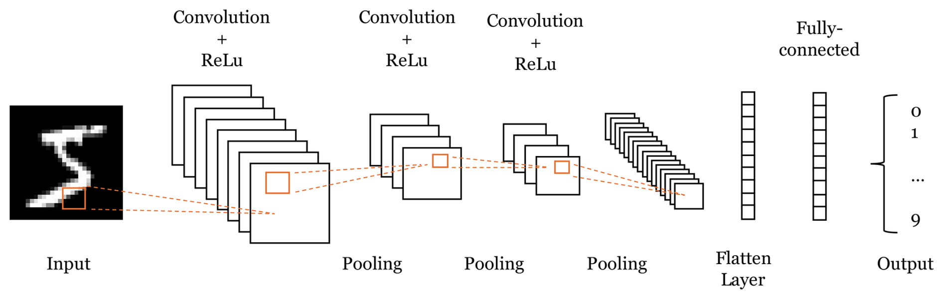
Figure 4 A simplified CNN architecture for an image classification task. The architecture is similar to the one of LeNet, which is an early CNN and was used for handwritten-digit recognition (Lecun et al., 1998).

3.11.2 U-Net

The U-Net architecture, introduced by Ronneberger et al. (2015), has become one of the most widely used neural networks for image segmentation. It was originally developed for biomedical applications, but it has proven versatile and has been adopted in a number of fields, including the remote sensing of the cryosphere (e.g., Ji et al., 2019; Mohajerani et al., 2021; Varshney et al., 2020; Donini et al., 2022a). Many variations of U-Net have also been proposed, each improving or adapting the design for specific tasks, such as ResUNet (Jha et al., 2019) and U-Net$++$ (Zhou et al., 2020).

The architecture features a U-shaped design, which consists of an encoder–decoder structure connected by skip connections. The encoder path down-samples the input image using convolutional and pooling layers, capturing high-level features and contextual information. The decoder path then up-samples these features, gradually restoring spatial resolution to generate a segmentation map. The skip connections link corresponding layers of the encoder and decoder, ensuring that high-resolution features from the encoder are integrated into the decoding process. This combination allows U-Net to segment objects with detailed boundaries, even in datasets with complex spatial structures (Ronneberger et al., 2015; Siddique et al., 2021). Figure 5 is an example of U-Net architecture for image segmentation.

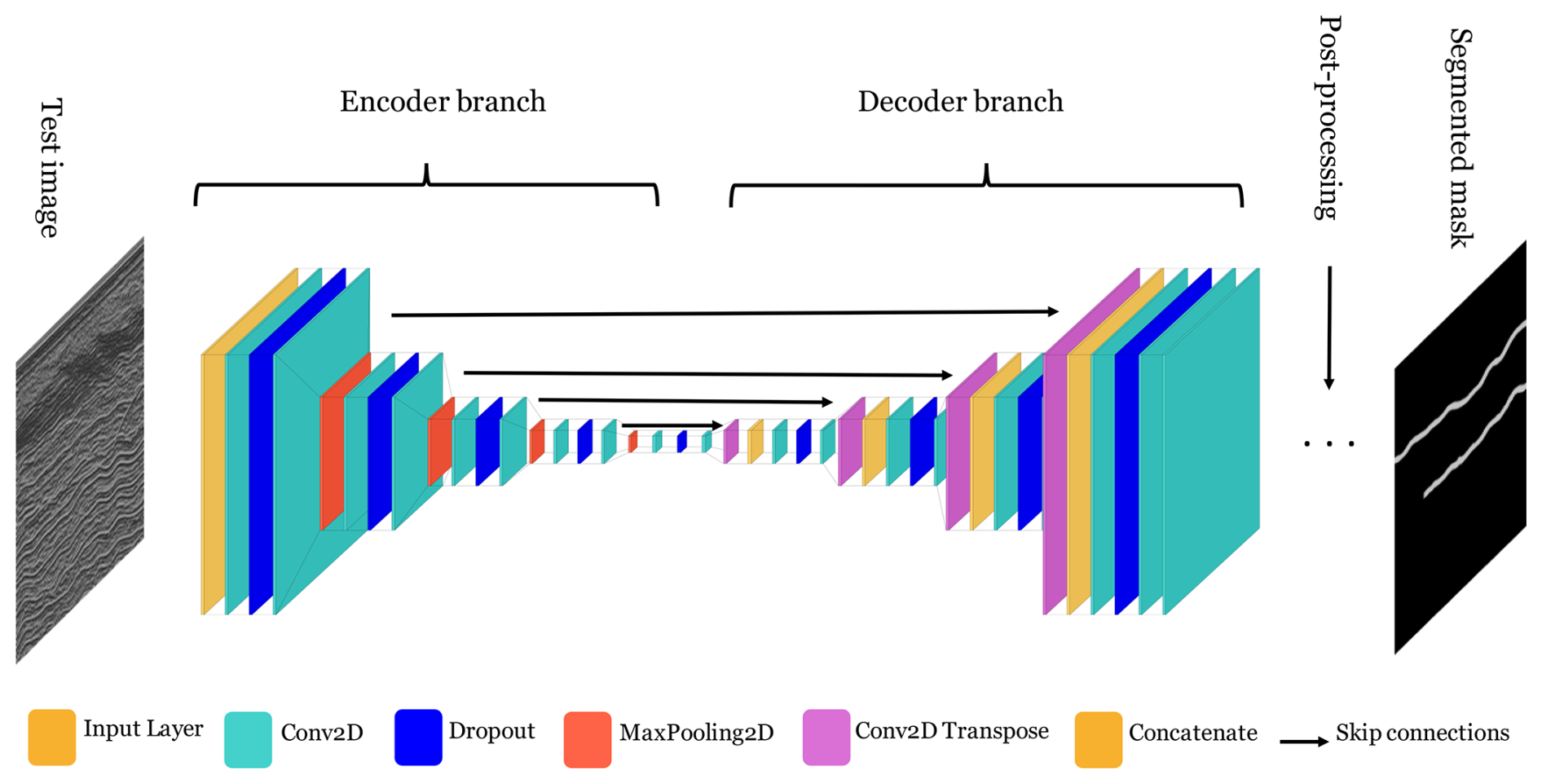
Figure 5 Schematic of a U-Net architecture and its conventional components, inspired by Ronneberger et al. (2015). Left- and rightmost images show a radargram and its representation with two IRHs predicted by U-Net.

3.11.3 Transfer learning and pre-training

CNNs typically require large datasets for effective training, which can be a significant difficulty when annotated data are limited (Lecun et al., 1998). Transfer learning provides a practical solution to this problem by allowing the use of pre-trained models as a starting point. This involves training a model on a large general-purpose dataset, such as ImageNet (Krizhevsky et al., 2017a), and then fine-tuning it using the smaller task-specific dataset available for the target application (Weiss et al., 2016).

There are a number of CNN models such as AlexNet (Krizhevsky et al., 2017b), GoogleNet (Szegedy et al., 2014), and ResNet (He et al., 2016) that are pre-trained on large datasets such as ImageNet. Pre-training on these datasets helps models to learn general feature representations that can be adapted to new tasks, which reduces the risk of overfitting and improves the robustness of the learning process (Hendrycks et al., 2019). This approach could be valuable in applications such as radargram analysis due to the scarcity of annotated training data.

3.11.4 Holistically nested edge detection

Holistically nested edge detection (HED) (Xie and Tu, 2015) is an end-to-end technique designed for edge detection that learns hierarchical features essential for understanding an image in its entirety (Long et al., 2014). HED is inspired by fully convolutional neural networks and incorporates deep supervision based on the Visual Geometry Group network (VGG-Net) architecture (Simonyan and Zisserman, 2014). Contrary to traditional edge detection algorithms that rely on abrupt changes in local pixel intensity, HED approaches edge detection as a holistic problem (global image-to-image mapping). Moreover, it uses side outputs, compensating for the absence of deep supervision which is a characteristic of fully convolutional neural networks. This design enhances the ability of the model to detect edges by investigating both local and global contexts.

3.11.5 Multi-scale learning

Multi-scale learning (Elizar et al., 2022) offers significant advantages using discriminative-feature representation to improve information acquisition. This is achieved through the fusion of low- and high-resolution data and the integration of diverse data sources. Multi-scale learning brings about a higher level of understanding the data and learning through collective results at different scales. The fundamental concept behind multi-scale feature learning involves the simultaneous construction of multiple CNN models with varied contextual input sizes. These models operate in parallel, and their respective features are merged at the fully connected layer (Elizar et al., 2022). An edge detection technique can be implemented at every scale for feature detection (Yari et al., 2020). For example, in radargram segmentation, small-scale structures may capture fine features, such as local fluctuations in layer boundaries, while larger scales focus on broader trends (Cai et al., 2022). Additionally, it is a feasible method to combine with other advanced networks, e.g., generative adversarial networks (Suh et al., 2022).

3.11.6 Recurrent neural networks

Recurrent neural networks (RNNs) (Cho et al., 2014) are designed to handle sequential data, such as sentences (Mirowski and Vlachos, 2015), time series (Hewamalage et al., 2021), and biological sequences (Aggarwal, 2018). Unlike other neural network architectures, where variables are independent of each other, RNNs process data in a sequential manner, with the input of each node being a combination of input and the hidden state from the previous time step (Goodfellow et al., 2016). In image segmentation applications, RNNs treat the task as a sequence prediction problem. This sequential processing is the strength of RNNs for image segmentation tasks (Salvador et al., 2019), making RNNs effective for tasks involving capturing relationships where a sequence is important.

4 Progression of IRH mapping and radargram segmentation techniques

In this section, we provide a concise description of the most important and relevant studies that have been done on mapping englacial stratigraphy. For the sake of simplicity, our timeline (Fig. 6) starts in the year 2000 to focus on more modern approaches. As Wang et al. (2020b) pointed out, at first the task of tracing IRHs from radargrams seems like a straightforward classic computer vision problem; however in practice it becomes obvious that it is a very challenging endeavor. Difficulties emerge for multiple reasons, such as high spatial variability, complex features, abundance of noise, an unknown number of horizons, and horizon discontinuity and merging.

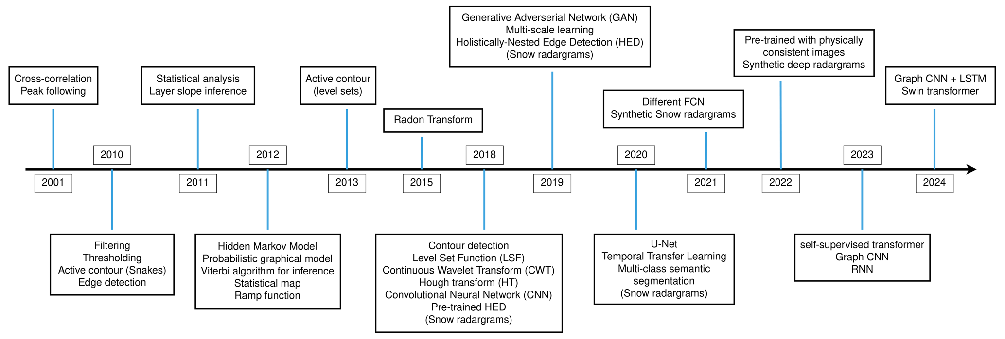
Figure 6 Evolution of selected methods for IRH tracing in chronological order, linked to the year each method was applied for the first time.

Over the last decade, various studies have put forth the use of pattern recognition methodologies in the examination of RES signals (e.g., Li et al., 2020). The primary focus of these investigations lies in the identification of specific subterranean entities, such as mines, pipelines, or tanks buried at shallow depths, through ground-based GPR. These entities mostly exhibit hyperbolic signatures in radargrams, a distinct contrast to most signatures in radargrams obtained from all platforms (ground, air, orbital) over ice. Consequently, we primarily abstain from including those investigations and their methodological proposals within the purview of this paper.

Automatic edge detection methods have been applied to a variety of applications of RES. Some of these include asphalt/pavement thickness measurements (Zhang et al., 2022), subsurface distress detection (Li et al., 2022), detection of structures beneath rail tracks (Peng et al., 2004), concrete feature tracking (Todkar et al., 2017), mine detection (Frigui et al., 2005; Reichman et al., 2017), and tunnel lining (Zeng et al., 2023). As for ice, this task is traditionally done manually or semi-automatically. Semi-automated methods include a certain degree of subjectivity. The two steps in which this subjectivity plays the main role are positioning of the seed points (to be connected to each other automatically) and critical evaluation of the results (Dossi et al., 2015). In recent years, there have been studies that have attempted to perform this task with automated methods. Such studies include a variety of approaches such as CNNs (Reichman et al., 2017; Zhang et al., 2022), Laplace transform artificial neural networks (Szymczyk and Szymczyk, 2015), and multilayer perceptron (Sukhobok et al., 2019), to name a few. However, as a result of radar systems differing in frequencies and waveform characteristics (thus resolution and penetration depth), studies applied to GPR and RES systems over mediums other than ice do not provide considerable insights. Therefore, the description of methods in our timeline (Fig. 6) concentrates on the studies that have focused on radargrams from ice sheets and other large ice masses, whether on Earth or planetary bodies.

In a number of studies, radargrams were analyzed to find different segments or subsurface targets (e.g., englacial boundaries, EFZ, basal units) and classes of events in each radargram (e.g., Donini et al., 2019; Goldberg et al., 2020; García et al., 2021, 2023). Even though we focus on the methods for mapping englacial ice structure and tracing IRHs and/or layer boundaries, we also take a look at studies done to detect regions and targets in radar products, since those are, in terms of methodology, in the close vicinity of stratigraphy mapping endeavors.

Table 1 gives a comprehensive overview of the published work for a quick lookup of published studies in tracing englacial stratigraphy. It contains published year, method(s) applied, traces mapped, and the type of radar system and the regions it was applied to.

Gades et al. (2000)Fahnestock et al. (2001)Gifford et al. (2010)Freeman et al. (2010)Reid et al. (2010)Ferro and Bruzzone (2011)Sime et al. (2011)Crandall et al. (2012)Ilisei et al. (2012)Smock and Wilson (2012)Ferro and Bruzzone (2012)Ferro and Bruzzone (2013)Karlsson et al. (2013)Mitchell et al. (2013a)Mitchell et al. (2013b)Lee et al. (2014)Panton (2014)Ilisei and Bruzzone (2014)Ilisei and Bruzzone (2015)Onana et al. (2015)Dossi et al. (2015)MacGregor et al. (2015)Koenig et al. (2016)Xiong and Muller (2016)Carrer and Bruzzone (2017)Xiong et al. (2017)Rahnemoonfar et al. (2017a)Rahnemoonfar et al. (2017b)Xu et al. (2017)Khodadadzadeh et al. (2017)Berger et al. (2018)Donini et al. (2018)Xu et al. (2018)Kamangir et al. (2018)Yari et al. (2019)Lines et al. (2019)Donini et al. (2019)Rahnemoonfar et al. (2019)Cai et al. (2020)Goldberg et al. (2020)Delf et al. (2020)Yari et al. (2020)Ibikunle et al. (2020)Keeler et al. (2020)Varshney et al. (2020)Wang et al. (2020b)Rahnemoonfar et al. (2021)Varshney et al. (2021b)Varshney et al. (2021a)Garcia et al. (2021)García et al. (2021)Donini et al. (2021)Khami et al. (2021)Varshney et al. (2022)Cai et al. (2022)Donini et al. (2022c)Donini et al. (2022b)Dong et al. (2022)Tang et al. (2022)Liu-Schiaffini et al. (2022)Ghosh and Bovolo (2022b, a)Ghosh and Bovolo (2023b)García et al. (2023)Ibikunle et al. (2023)Atefeh Jebeli et al. (2023)Zalatan and Rahnemoonfar (2023)Varshney et al. (2023)Ghosh and Bovolo (2024)Liu and Rahnemoonfar (2024)Peng et al. (2024)Moqadam et al. (2025)

Table 1 Published research on mapping methods.

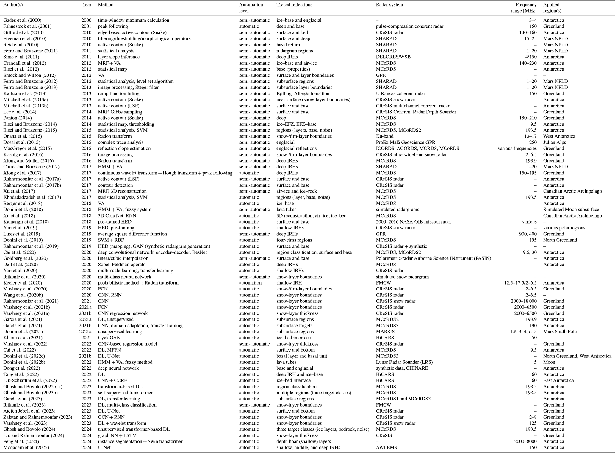
Note that the MCoRDS radar was developed by CReSIS. We use the same terminology for referring to the radar system as used in the original publication.

We present published studies classified into three main categories of methods, labeled with their respective subsection number:

• 4.1

  Computer-vision-based and signal processing methods. This category consists of filtering and thresholding methods, peak following, layer slope inference methods, transform methods such as Radon and wavelet transforms, and active contour methods.

• 4.2

  Probabilistic and statistic methods. This consists of Markov methods, Viterbi, statistical mapping, support vector machine, and Gibbs sampling.

• 4.3

  Deep learning methods. This includes CNN-based models and related architectures and modifications.

In the following subsections, we present published studies within these three main categories, grouping connected works in individual paragraphs. Furthermore, the citations in italics indicate the main reference considered in the summary paragraph. For studies which employed multiple approaches, we have included each in the category to which its main method belongs. It should be kept in mind that categorization in separate groups mainly serves readability and coherence and does not indicate strict separation between categories.

4.1 Applications of traditional computer vision and signal processing methods

Gades et al. (2000) and Nereson et al. (2000) have both employed a semi-automatic picking routine for bed and deep horizons, respectively. Their method finds the maximum amplitude of each of the RES traces in a prescribed time window. Their pre-processing step is the noise removal using a fourth-order Butterworth band-pass filter. Similarly, Fahnestock et al. (2001) used peak following and cross-correlation and applied them to the pulse-compressed coherent radar data. Peak following was used to select and follow IRHs on the radargrams taken by the NASA radar system. This method is mainly automatic; however there is an operator-assisted element to ensure accuracy. Radargrams were visually improved by normalizing them from the depth of 400 m and lower in order for the operator to better identify the reflections. The authors remark that peak following is the method of choice for areas where peaks are distinctly visible but patterns are ambiguous. The correlation method, in contrast, is more suitable for instances where peaks are faded and patterns are more distinct. Lines et al. (2019) present a hybrid method founded upon Fahnestock et al. (2001) to track the IRHs in radargrams covering the snow and firn columns. These interactive semi-automatic methods seem to be sensitive to noise, acting as a weakness for GPR data. The method is called the average square difference function layer picking system (ALPS), named after the algorithm it uses for tracing IRHs. Connecting discontinuities that exist in radargrams, especially near crevassed terrain or close to the ice sheet margin, is a weakness of this method.

In the planetary ice sheet domain, Freeman et al. (2010) implemented a method to detect near-surface ice layers in Mars' ice-rich northern polar layered deposits (NPLD) from radargrams of the Shallow Subsurface Radar (SHARAD) mounted on NASA's Mars Reconnaissance Orbiter. SHARAD radargrams are equipped with linear frequency modulation (LFM), which operates in the range of 15–25 MHz. SHARAD's products are often used for tracing or segmenting IRHs and regions of ice. As a pre-processing method, the authors use a Gaussian blur and a high-pass filter. The main techniques for detecting IRHs are thresholding and morphological processes.

Gifford et al. (2010) used the edge method and edge-based active contour to pick the surface and basal reflections in an attempt to estimate the thickness of ice sheets. To estimate the ice thickness, one needs two reflections: the first peak representing the ice surface and the last peak representing the base. These two peaks are the strongest in the vicinity of every individual trace. The authors list some of the shortcomings of traditional segmentation methods for this task such as watershed (Beucher and Lantuejoul, 1979), level set (Chunming Li et al., 2011), and region growing (Pal and Pal, 1993) methods. The main reason for these shortcomings is that the base reflection of an ice sheet is neither reliably continuous nor connected, e.g., in regions with steep topography of very thick ice (> 4 km). Other obstructions are the presence of noise and the non-uniformity of the characteristics of ice sheets because of the deep reflections and surface multiples. Furthermore, the basic edge detection techniques suffer from a lack of continuity, stiffness, and smoothness, which makes them not optimal stand-alone choices for this task. The authors applied their approach to the data from the University of Kansas, the Center for Remote Sensing of Ice Sheets (CReSIS). They present a visual comparison of the basal horizon picked by (1) a human expert, (2) an edge-based approach, and (3) an active contour approach. It is concluded that the active contour method provides the best approximation of the base, with a trade-off in terms of time, as it takes longer compared to the edge detection method for the contour to end up on the basal reflection. The advantage of the active contour over the edge-based approach mostly lies in its ability to bridge the discontinuities. However, the weakness of the active contour seems to be in regions where the texture below the base is rough or where strong IRHs or other reflection signatures occur near the ice sheet base (Gifford et al., 2010). Automatic mapping of the air–ice and ice–bed boundaries is a task which has been tried by various studies throughout the years to calculate surface or basal topology or ice thickness. Reid et al. (2010) used two different methods to map the ice surfaces and basal reflections, aiming to estimate the ice thickness, in a manner similar to techniques presented by Gifford et al. (2010). They applied their implementation to data from CReSIS and concluded that although edge-based methods are faster than the active contour method, the latter is more robust to image artifacts and yields better continuity in traced IRHs. One interesting suggestion is that the edge-based methods can be used as the initialization for the active contour method.

Sime et al. (2011) used an automated finite-segment method to obtain englacial reflector dip angles, from both airborne and ground-based radar observations. In fact, this is not an interface-picking method, as dips are horizontally integrated to produce synthetic isochrones. Integration of the slope of local layers yields a first-order approximation of the layer location. The method is a horizontal averaging technique that reduces the noise and identifies the layers but does not attempt to trace complete horizons. Similar approaches, e.g., that of Holschuh et al. (2017) on computing slope information from radargrams, have further improved our understanding of the inner structure of the ice sheets.

Ferro and Bruzzone (2013) focused on automatic characterization of the linear features in radargrams taken from Mars NPLD. They considered some previous studies employing the Hough transform for radargrams (Gamba and Lossani, 2000; Pasolli et al., 2009) to be useful for detecting hyperbolae or straight lines. Nonetheless, the efficacy of such approaches decreases significantly when applied to radargrams, which include features that are not straight; this is also the case with GPR products from glacier ice. The output is a vector object described by its local width, and computing features' geometrical characteristics without further post-processing is possible. The method is composed of a combination of some image processing techniques, namely pre-conditioning, block matching and 3D-filtering processes (BM3D), to remove the noise and subsequently a Steger filter (Steger, 1998) for ridge detection. For denoising, the main filter used is BM3D (Dabov et al., 2007), which, while removing noise, preserves linear features (Ferro and Bruzzone, 2013). It is worth mentioning that this and similar studies that investigate planetary data are subject to different types of noise and radiometric characteristics compared to data taken from aircraft or on terrestrial ice sheets.

To investigate the depth of the Bølling–Allerød interstadial, an important warming event of the last deglaciation, Karlsson et al. (2013) presented an automatic fitting method. Having dated the transition at an ice-core drill site, they extended this transition further away from the ice-core site. They noticed that the upper half of the radargrams from CReSIS RES data from Greenland contains many more reflections than the lower one, and they subsequently fit a ramp function to represent the standard deviation of the data. They constructed the data histogram using an optimal number of bins and reconstructed the radargram using intensities of the mean values of each bin. They then fit a 2D version of the ramp function to the more interesting parts of the reconstructed radargram. Finally, the location of most of the fits was selected as the depth of the transition. They concluded that the absence of the transition is the result of ice flow having disrupted the layering (Siegert et al., 2004) and that it is not possible to recognize layering in thin ice (Fahnestock et al., 2001).

Mitchell et al. (2013a) used the method proposed by Steger (1998) to find the estimated position of the curves belonging to horizons. They combine off-the-shelf methods to estimate near-surface layers in radargrams of the snowpack. They find points with high probability of being part of curvilinear structures, and therefore, the features are more parallel and less fluctuating. A user is required to initially determine the number of visible layers. The pipeline starts with edge detection to estimate the layer location, curve point classification to estimate reflection location, and finally an active contour (Snake) to distinguish lower reflections from the upper ones. They noted that the Canny operator is only suitable for identifying near-surface and not deeper reflections due to fainter layers boundaries and inherent noise of the radargrams. Panton (2014) introduced two methods that infer the local slope and track a boundary, respectively, from the initial estimate. The methods trace IRHs by optimizing the position of the entire IRH to improve the areas with poor radargram quality. After pre-processing, local boundary slopes are estimated and seed points are picked by a human expert. From here, the Snake algorithm traces the boundaries from the picked seed points. In areas where there are discontinuities in the IRHs, for instance in the presence of shear margins or disturbing fast flow, the method yields incorrect slope fields; therefore it is not recommended for areas where stratigraphy is visibly complex. In a similar work, Mitchell et al. (2013b) also employed LSF to semi-automatically estimate the surface and basal interface from a multichannel coherent radargram. An expert provides two initial contours for the air–ice and ice–base boundaries. These lines then evolve at each step while a cost function is calculated, and this continues until the cost function reaches a minimum using gradient descent. This method was applied to 20 radargrams and provided a comparison between this approach and the HMM approach of Crandall et al. (2012), and it was shown that level set performs between 3 and 5 times better than HMM for air–ice and ice–base boundaries, respectively. Rahnemoonfar et al. (2017a) also used a LSF method to detect the topology of surface and basal boundaries. They tested the approach on 323 radargrams from NASA's Operation Ice Bridge (OIB) mission and iterated 800 times from the initial curve to overlap with the air–ice and ice–base boundaries. The difficulties of processing air–ice and ice–base boundaries are classified as follows: (i) subglacial topography is greatly variable; (ii) there are artifacts in the data, mainly a result of electric devices around the radar as well as the aircraft itself; and (iii) ice–base boundaries exhibit low signal-to-interference-and-noise ratios (SINRs). In another study, Rahnemoonfar et al. (2017b) detect air–ice and ice–bed boundaries inspired by Coulomb’s electrostatic law based on the projection profile of the contours. IRHs are interpreted as contours. The grayscale intensity of a pixel symbolizes the electrical charge associated with each particle. By establishing specific criteria that translate electrical charges into pixel characteristics, the resulting computation of the electric field for each pixel is used to define the edges within the radargram. To remove noise, an anisotropic difference is applied.

The Semi-Automated Multi-layer Picking Algorithm (SAMPA) introduced by Onana et al. (2015) is an algorithm that traces annual accumulation layers from firn radargrams from both airborne and ground-based radar systems. A Radon transform is used to map the features which represent firn-layer boundaries, which are later traced using thresholding of the amplitude. SAMPA was applied to radargrams from West Antarctica where the firn layers are known to be rather flat. Deeper boundaries are more difficult than shallow ones for SAMPA to trace because of attenuation and low contrast resulting from low variance in trace amplitude. Xiong and Muller (2016) mention that the difficulty of tracing internal IRHs is due to the presence of non-contiguous IRHs, and they relate that to local anomalies such as folds and crevasses caused by ice dynamics. The underlying method here is also the Radon transform, similarly to Onana et al. (2015), to extract IRHs from radargrams of NEEM station. However, the authors note that Onana et al. (2015) extracted firn IRHs which are represented as horizontal lines in radargrams, and in this study, the goal was to also extract deeper IRHs with larger slope bending. Therefore, they adapt SAMPA, which is based on block processing, and convert it to slice processing. They present a comparison of the two methods in one radargram and conclude that the present method functions more effectively, especially for deeper IRHs. It is worth mentioning that the only measure of effectiveness presented is qualitative. Continuous wavelet transform as a strong signal processing tool was used together with Hough transform (Ballard, 1981) by Xiong et al. (2017) to semi-automatically trace IRHs and infer the local dips and propagate them away from the CWT seed points. The critical problem with peak following is that there is a high possibility of falling onto neighboring layers. Moreover, in determining which pixels/regions might constitute peaks and which might not, they note that high-amplitude peaks do not always correspond to layers, while, conversely, low-amplitude points can indeed signify peaks. A post-processing algorithm is triggered that connects the lines that belong to each other. The authors compare their results with those of MacGregor et al. (2015) and show that more horizons were traced using CWT and Hough transform. This is related to the fact that seed picking in the method of MacGregor et al. (2015) was done manually, and consequently only prominent horizons were picked. For instance, IRHs around folds are not picked in the Radiostratigraphy and Age Structure of the Greenland Ice Sheet (RRRAG) dataset (MacGregor et al., 2015). There is good agreement between their result and the published RRRAG radiostratigraphy dataset, while the average vertical difference (between the traced IRHs of the two methods) is 15 pixels, which corresponds to 40 m.

Phase information has also been useful in developing IRH tracing methods. Dossi et al. (2015) developed a method to detect and trace reflections with lateral phase continuity and to assess polarities (to evaluate the materials) in GPR and seismic data using attribute analysis (Taner et al., 1979). As any single reflection is the outcome of a series of phases with alternating polarities, it is difficult to determine the initial phase, i.e., polarity. The method is rooted in automatic identification of the reflection phase using the cosine of the instantaneous phase and search for sub-parallel events, in other words, tracking events whose phase continues laterally. The cosine phase of signals was employed to reconstruct the reflected wavelet's shape. Synthetic GPR data created with GPRmax (Giannopoulos, 2005) were used for testing the method, in addition to real data from Alpine glaciers and archaeological surveys. Similarly to other methods, it was found that a limitation of polarity assessment is that there exist many closely spaced parallel reflections and these could be recognized as single events. As with intensity gradient methods, including a thresholding step is a necessity to select only stronger events. The method is able to pick numerous short-length horizons but falls short in dealing with discontinuities, in a manner whereby the method picks up phases of unrelated events as a single horizon. MacGregor et al. (2015) introduced two interactive semi-automatic methods to predict internal stratigraphy based on phase information as well. They rely on calculating reflections' slopes, similarly to the works of Sime et al. (2011) and Panton (2014). Integrating the slope in the along-track direction yields the stratigraphy (predictions). The first method uses the smooth horizontal phase changes along the radar track and the natural coherence of radar signals to predict reflection morphology, benefiting from recordings of coherent radar while implementing SAR techniques as a backbone (Raney, 1998). The second method calculates the reflection slope by extracting information from the wavenumber of the Doppler centroid in radar data. Fourier transforms are computed on brief segments of radar data to examine the Doppler spectrum of englacial reflections. Goldberg et al. (2020) developed an algorithm to detect basal units. They introduced a SAR processing method and employed unique phase shift response functions to classify feature types such as englacial layers and potential basal units. The method can distinguish between feature types by matching model phase shift responses to pixel data.

Noise removal is the initial step for most of the methods, such as that of Koenig et al. (2016), who applied a median filter to remove noise and detected the snow surface simply by thresholding. They devised a semi-automated snow-layer boundary detection algorithm and applied it to radargrams from NASA's OIB Arctic campaign taken from 2009–2012 and surveyed by CReSIS' ultra-wideband snow radar. Identification of peaks is facilitated by the distinction between spatial variability in the travel-time–depth domain across high and low frequencies, functioning as a high-pass filter. These identified points are subsequently linked to form coherent IRHs by utilizing the half-maximum width of the waveform associated with each peak. After connecting the picked points using spline fitting, an expert examines the picked IRHs by correcting indices, filling gaps, deleting, adding, and performing other corrections.

Delf et al. (2020) performed an inter-comparison of automated IRH tracing and layer-dip-estimation methods. In order to asses their capabilities, two types of algorithms were implemented: those that trace IRHs and those that extract the slope or dip of the horizons; and their capability to propagate an age–depth model was tested. The authors used two CReSIS Multichannel Coherent Radar Depth Sounder (MCoRDS) datasets from Antarctic ice sheet surveys for the inter-comparison study and implemented three algorithms: (i) the Automated RES Englacial Layer-tracing Package (ARESELP) implemented by Xiong et al. (2017), (ii) the Steger algorithm implemented by Ferro and Bruzzone (2013), and (iii) the Sobel–Feldman operator (also called Sobel; Sobel and Feldman, 2015). To assess each method, its impact on propagation of a simple age–depth relationship (Nye, 1963; Leysinger Vieli et al., 2007) was investigated. The central conclusion was that there is a requirement for further studies and advances in such algorithms, as even in a region with relatively simple geometry, the methods do not show promise in linking age–depth profiles between two locations. It is important to note that all three methods performed better in dip estimation compared to their performance in IRH tracing.

4.2 Applications of probabilistic and statistical methods

Smock and Wilson (2012) developed a layer boundary detection identification algorithm for GPR radargrams captured by vehicle-mounted sensor arrays. Their work is an extension of Smock et al. (2011). Finding base and surface reflections in radargrams was implemented using VA, representing radargrams as trellis graphs. To investigate subsurface layer boundaries, one has to look for multiple disjoint paths through the trellis graphs. The authors propose a criterion for choosing multiple disjoint paths called a reciprocal pointer chain. However, due to lack of ground truth, no quantitative comparison was provided.

The statistical analysis by Ferro and Bruzzone (2011) presents a method to detect scattering areas of a radargram, namely the basal returns. The data are from SHARAD in a lower frequency range of 1–20 MHz. The authors classified radargram regions, such as strong layers, weak layers, no target, and basal layers. For each of these classes, they analyzed the statistical distribution of their corresponding returns by means of fitting three pdf's, namely the Rayleigh, Nakagami, and K pdf's. Using maximum likelihood, the parameters of these pdf's for each class type were estimated. For evaluation, they calculated the root mean square error (RMSE) and the Kullback–Leibler divergence (Lin, 1991) between the normalized histogram of data and the obtained histogram. The best fit is shown to be the K-pdf distribution in almost all the cases. The product of the method is used to calculate the NPLD thickness, local geology, and seasonal variations. To ascertain a selection of statistical distributions capable of characterizing amplitude variations caused by distinct subsurface categories, Ferro and Bruzzone (2012) analyzed radar sounder products from Mars NPLD once more with two main objectives. One is computing statistical properties of radargrams, and the other is devising two methods for automated extraction of subsurface features. They previously found that the signal statistical distribution pertaining to different targets can be modeled efficiently using the K-pdf distribution and that the background noise can be modeled by a Rayleigh distribution (Ferro and Bruzzone, 2011). They generated a map for the different subsurface classes and additionally identified and mapped the deepest scattering areas. They considered their approach to be a first step for a general framework for analysis of radargrams.

Crandall et al. (2012) proposed finding boundaries between layers of different materials (such as air, ice, or rock) in radargrams as an inference problem on a statistical graphical model using Markov random field (MRF), HMM, and VA (Crandall et al., 2012). This inference model includes a number of constraints, such as layer boundaries being located where there are high radargram contrasts, being continuous, and not intersecting with others. The hidden variables are pixels that belong to an IRH, and VA is supposed to return the maximum likelihood path of the HMM. The authors used 827 radargrams with a size of 700 × 900 pixels from NASA's OIB mission as test data. These radargrams were manually labeled as well, serving as ground truth. They divided their dataset into a training and test set with almost 50 % for each set. The method showed better results for identification of the air–ice interface and could pick these IRHs in a rather short time. By adding the constraints and human interaction, the error was decreased to some extent. One notable advantage of probabilistic models is their robustness against inherent radar noise. Lee et al. (2014) also considered the task of tracing air–ice and ice–bed boundaries as a probabilistic inference problem and used a Markov chain Monte Carlo approach to sample from the joint distribution over all the possible layers in each radargram. The advantage of this approach is that it brings multiple possibilities of integrating over and obtaining the layer boundaries, as opposed to edge detection techniques, which present hard singular boundaries. IRHs are computed from expectations of the distributions, and confidence intervals are computed from the variance of samples. The Gibbs sampling is used due to its ability to characterize uncertainties by calculating confidence intervals. The authors show that their method yields an improvement over the approach of Crandall et al. (2012). The challenges are the presence of noise, faint reflections between boundaries, and the confusing structure that is a result of signal reflections and clutter. Random noise prevents correct picking because of serious signal distortion. Xu et al. (2017) aimed to reconstruct a 3D structure of the ice sheet from available 2D profiles. They approached this as an inference problem and employed a probabilistic graphical model, namely MRF to resolve the reconstruction. This model searched for a surface that minimizes a discrete energy function on a first-order MRF. This study took advantage of 3000 radargrams for each of the seven topographic sequences which were resolved, corresponding to 50 km. Results were compared to the extruded results of Crandall et al. (2012) and Lee et al. (2014), showing that the Xu et al. (2017) study presented a more robust method. Berger et al. (2018) worked on modifications to the previous methods (Crandall et al., 2012; Xu et al., 2017). They assumed that the surface boundary was known a priori, and the focus was on the extraction of the ice–base boundary. Another useful assumption was that the interface between ice and base was single-valued in the radargram, which meant that every column of the radargram could only contain 1 pixel belonging to this interface. By trial and error, they concluded that the optimum result was obtained for 50 iterations. The modified Viterbi algorithm achieved a significantly improved performance and made the method more appropriate for a wide range of radargrams, based on comparison with results of Crandall et al. (2012), Lee et al. (2014), and Rahnemoonfar et al. (2017a) in terms of absolute column-wise difference.

To calculate ice thickness and basal properties, Ilisei et al. (2012) used the MCoRDS data to construct a statistical map that accentuates the predominant subsurface features within the ice. The map was subsequently partitioned, facilitating the identification of regions associated with basal scattering. Additionally, the method identified the surface, thereby enabling precise ice thickness computation. The map was segmented into distinct sectors such as the base, englacial fold zones, and englacial layers. It was applied to seven radargrams that had been pre-processed using the minimum variance distortionless response (MVDR) approach. Manual initialization is integrated into the procedure, rendering it a semi-automatic method. Weaknesses are presented as (i) results depending on the presented model of the radargram (not usable for other radar systems) and (ii) the method using spatial correlation of the subsurface features. To recognize specific ice subsurface targets and estimate their characteristics, Ilisei and Bruzzone (2014) suggested a semi-automatic method based on statistical map generation. It is based on a comprehensive understanding of the statistical attributes of the radar signal and the spatial arrangement of subsurface targets. Firstly, a statistical analysis of the radargram was performed to yield a statistical map of it. This was followed by thresholding and segmenting this map into the areas of interest (horizons, noise, EFZ, and base). Having the same objectives as Ilisei and Bruzzone (2014), Ilisei and Bruzzone (2015) proposed a different method to obtain specific subsurface targets, applying feature extraction and automatic classification consecutively. The features were extracted using statistical analysis, similarly to Ferro and Bruzzone (2012), and spatial distribution of subsurface targets. The classification was performed using the SVM classifier (Cortes and Vapnik, 1995). They performed statistical analysis by fitting pdf's, as well as other manually designed features, such as parameters of the best-fitting statistical model, texture (entropy), and a statistical distance measure (Karhunen–Loève (KL) divergence). The next step was to obtain an approximation of the location and spatial distribution of the classes, e.g., the expected order of the classes and their extension in the along-track direction. Once these targets and their features were known statistically, this information was preserved as input to an SVM for predicting regions in unseen radargrams. SVM was chosen mostly thanks to its capabilities in generalization and non-linearity comprehension. The technique has proven to be robust in handling radargram heterogeneity, as a result of the integration of both statistical and machine learning methodologies. Moreover, SVM is capable of objective extraction since the same criteria for feature extraction were used for all radargrams. Furthermore, it is possible to parallelize the method and it can perform at high speed. Another attempt to classify various englacial regions was made by Khodadadzadeh et al. (2017). The novelty of this work lies in the fact that the window for region classification is not fixed but its size is adaptively changed with regard to characteristics of englacial structure in order to classify the radargram into ice, base, and noise. Using this adaptive window, the method is able to extract features from a radargram via piecewise constant representation of the backscattering signal in the vertical direction to adapt the window size. These extracted features were used in an SVM to perform the classifications in the same way as in Ilisei and Bruzzone (2015). The authors compared their results to their previous work (Ilisei and Bruzzone, 2015) and observed an improvement.

Shifting from classifying regions, ice base, and ice surface IRHs to tracing internal IRH, Carrer and Bruzzone (2017) used radargrams taken from Mars NPLD by SHARAD and implemented a method to automatically trace (shallow and deep) IRHs. Their approach uses a combination of local-scale HMM and VA. Detection of IRHs involves inferring the most probable boundaries within a section of the radargram, employing an algorithm to patch together local IRH locations. Furthermore, a radargram enhancement and denoising technique are introduced. One issue with VA is that when two IRHs are very close to each other, it mistakenly interprets them as one layer and might jump from one to the other while tracing. To facilitate the comparison, the same radargrams as those of Ferro and Bruzzone (2013) were used. Similarly to Ferro and Bruzzone (2013), the authors investigated the upper part of the radargram as it is the shallow region near the surface where the spatial density of the IRHs is high. The high computational complexity caused by large IRH density and long-azimuth acquisition is resolved by the divide-and-conquer approach; i.e., the radargram is divided into blocks, within which both inference and discrimination between noise and layer boundaries are conducted. For the ultimate purpose of finding an alternative place to Earth for humans, the Moon has been investigated and lava tubes have been proposed to be an optimal place for human habitat. Donini et al. (2018) developed a method to detect such features using analysis of radar sounder data. Their method is composed of two steps: (i) extraction of linear features from radargram amplitude and phase using the method of Carrer and Bruzzone (2017) (HMM + VA) and (ii) evaluation of features using a fuzzy-logic-based system in order to detect the tubes. Another attempt to automatically detect subsurface lava tubes on the Moon was performed by Donini et al. (2022b). A fuzzy system that extracts these tubes on the basis of their geometrical features in radargrams is utilized. The method is an extension of that of Donini et al. (2018). It is an unsupervised method, and the analysis itself is a fuzzy detection system. The steps include firstly improving the signal-to-noise ratio using a conditional density function (CDF) of the noise and the signal, then using HMM and VA to detect the lava tube signatures. Eventually, a fuzzy-logic-based system analyzes the extracted lines in the radargram.

With the aim of categorizing radargrams into four distinct regions – ice layering, refreezing ice, base, and the EFZ and thermal noise – Donini et al. (2019) proposed a method for radargram segmentation. The class termed “refreezing ice” refers to liquid water, which creates a particular structure when it is in contact with ice and accretes to the overlying ice at the ice–bed interface (Carter et al., 2017). The labeled samples are described by a set of features that discriminate between the different structures present in the radargram. The segmentation process involves applying a pixel-based classification using an SVM classifier with a Gaussian radial basis function (RBF) kernel. The classification is supervised, meaning that the classifier learns the characteristics of the different classes from a set of labeled samples selected from the radargrams. The authors performed cross-validation to determine the optimal parameters for the RBF kernel of the SVM classifier. Once the classifier is trained, it assigns a label to each pixel of the radargram based on its learned characteristics. The resulting segmentation map shows the distinct regions of the radargram, categorizing the different geological structures and noise present in the data. The algorithm was applied to radargrams obtained in northern Greenland and showed high accuracy in mapping the refreezing ice.

Keeler et al. (2020) devised a fully automatic probabilistic method to estimate the surface mass balance from radargrams. The method primarily utilizes successive peak following and Monte Carlo simulations. The authors present the Probabilistic Automated Isochrone Picking Routine (PAIPR), with the aim of estimating annual surface mass balance in the upper 25 m of dry firn. The data are obtained by a frequency-modulated continuous-wave (FMCW) radar, both ground-based and airborne. After amplifying the signal-to-noise ratio, the layer gradient field is estimated using a local Radon transform with a moving window. The next step is to find peaks and subsequently group them together to form IRHs. Afterwards, they assign the likelihood of isochrones using a logistic regression algorithm. Lastly, the age–depth scale for each of the picked layer boundaries is estimated. After comparison with the method of Onana et al. (2015), it is concluded that this study presents a more robust method. Furthermore, some of the limitations of the presented method are stated, one being that it requires radargrams which are taken from spatially longer sections.

4.3 Applications of deep learning methods

In this subsection, summaries and the main points of the studies that used deep-learning-based methods are presented. We would like to note that although the primary focus of some of the works, e.g., Donini et al. (2021), Donini et al. (2022c), Garcia et al. (2021), García et al. (2023), Ghosh and Bovolo (2022a), and Ghosh and Bovolo (2023b), lies in radargram region segmentation, they are included in this review because of their methodological relevance for the overall objective.

To perform the same task as Xu et al. (2017), i.e., 3D reconstruction of the ice sheet using 2D radargrams, Xu et al. (2018) present a DL-based method for tracing basal or englacial IRHs. A multi-task spatio-temporal neural network that combines 3D ConvNets and RNN is constructed. The specific RNN is comprised of gated recurrent units (GRUs), commonly used for learning sequential data, which are coupled to a convolutional 3D (C3D) network (Tran et al., 2014). The authors' dataset and study regions are the same as those of Xu et al. (2017). Comparison with Crandall et al. (2012) and Lee et al. (2014) shows that the approach achieves better results, as methodologies of those studies were designed for 2D segmentation. Additionally, another comparison with Xu et al. (2017) concludes that the approach yields slightly poorer results because Xu et al. (2017) utilize more information, i.e., additional non-visual data such as prior weak information about ice thickness information from satellite maps. However, without this information, the study yielded more accurate results. Also, the method is much faster than that of their previous study (Xu et al., 2017) as the former method rests on statistical analysis. To further evaluate the method, the authors ran several baselines to gauge the different components of their architecture, observing that all the components play a vital role in the final outcome.

To trace the ice–air and ice–bed interfaces, Kamangir et al. (2018) initially applied an undecimated wavelet transform for removing speckle noise from the radargrams due to its translation invariance. The next step is a multi-step neural network to extract the edges from the radargram. The architecture is a pre-trained HED, built from a series of convolutions. After each set of convolutions, there are two outcomes, one of which goes through a max pooling step and next step of the convolution (thus shrinking in size) and another one that is taken as a side output. These independent networks combined with the result of each side output form the final output of the model. Yari et al. (2019) used NASA OIB ICE2012 data to implement a multi-layer learning HED to map the shallow IRHs. Three experiments were performed: (i) using a pre-trained model, (ii) training on a synthetic radar dataset, and (iii) training with a normal distribution initialization. Pre-training was performed on the BSDS500 data (Martin et al., 2001) and their augmentation (Arbeláez et al., 2011). Even though transfer learning seems to be a good approach, because most neural networks are trained on optical imagery with much less noise, the pre-training approach yielded poor results or did not converge overall. The synthetic dataset uses a simple linear superposition for IRHs, and a layer thickness model generated by a smoothed Gaussian random process produces a simplified and not very realistic dataset. Thus, training on synthetic data did not return acceptable results either. It was concluded that training a model from scratch gives the best results out of the three.

To synthesize radargrams, a generative adversarial network (GAN) (Goodfellow et al., 2014) was used by Rahnemoonfar et al. (2019), and later an HED model was trained using this synthetic dataset. The authors noted that such radargrams cannot completely replace the use of real radargrams for training since they do not contain all characteristics of real radargrams such as noise and the Doppler effect. Along with quantitative tests, a qualitative test was undertaken to evaluate the produced radargrams, which resulted in synthetic and real radargrams being indistinguishable to the observers. After training an HED network for tracing englacial boundaries, it was observed that the network's results improved when trained with actual and synthetic data. Due to their inability to reproduce nuances of real radargrams, training solely on synthetic data cannot produce high-quality results. The best results came from the experiment with an equal number of synthetic and real radargrams for both training and testing, and the worst came from a combination that was trained on synthetic radargrams and tested on real ones. An important conclusion is that while synthetic data are visually and statistically similar to real data, they fail to represent the physics. Khami et al. (2021) also used GAN to remove strip noise and confine layers in RES data. To remove the chance of the model learning implicit assumptions of operators for filtering criteria, they chose an unsupervised approach to GAN called CycleGAN. This is a GAN network for image-to-image translation between two unpaired domains (Zhu et al., 2017). CycleGAN requires two sets of data. In this study, they have used one real-world unfiltered dataset and one synthetic dataset (on the basis of Hall et al., 2015). The framework consists of two generators, each of which learns to translate images to the domain of the other generator and subsequently feeds the output to the other generator. One generator receives real unfiltered radargrams (HiCARS version 1 radar data; Blankenship et al., 2017), with strip noise, and the other one receives synthetic dataset, with clear but simple stratigraphy. This unsupervised GAN was chosen because of the limited number of paired noisy and interpreted radargrams available for training. Their model was rather effective in tracing the ice–bed interface in radargrams with minimal strip noise. However, with larger amounts of strip noise, it was not successful. Their synthetic data also prove to be inadequate in representing transitions as details at the ice base in the radar data are removed.

Cai et al. (2020) developed a framework performing pixel-level classification using a deep convolutional classifier with the goal of classifying the englacial regions of ice sheets. The network architecture is composed of filter processing and an encoder–decoder. For training and validation, radar products provided by CReSIS are used. Their initial stage is to remove the noise using bilateral filtering. The encoder contains atrous spatial pyramid pooling (ASPP), whose function is to improve classification and obtain multi-scale feature extraction, and the backbone network is the ResNet3 (He et al., 2016). In the decoder, high- and low-level features are proportionally concatenated so that the low-level edge information can be used. The model manages to yield the same F measure as Kamangir et al. (2018).

Ibikunle et al. (2020) used a multi-class neural network and the iterative “row–block–column” approach and presented their preliminary results for automatically tracing the snow-layer boundaries from snow radargrams of CReSIS. They simulated the training data, which are considered to not capture all the details of real radargrams in snow but nevertheless show some promise for training. The iterative approach starts from the known IRH using the rows below it and continues in the direction of deeper snow boundaries. Using the same iterative approach, Ibikunle et al. (2023) enhanced their previous work and trained a multi-class classification deep neural network to identify the index for the next layer boundary in each column, using a RowBlock approach. A “columnpatch”, which is the N neighboring columns of the current column under the iterative process, is used to enhance robustness and spatial awareness of the algorithm. Since this method is grounded in selecting a number of rows beneath each known IRH, it is methodologically inappropriate for deeper boundaries and suitable only for snow-layer boundaries. Firstly, the deeper in the radargram one goes, the steeper variability there is in the geometry of the boundaries. Secondly, owing to layer compaction from overburden pressure, the deeper IRHs are closer to each other, making it much more difficult to choose a suitable number for each row block.

Acknowledging that automatically tracing englacial IRHs is much more challenging than detecting the ice–base boundary, Wang et al. (2020b) implemented a CNN to detect the surface boundary, estimate layer thickness, and estimate the number of visible IRHs. They frame the task as a tiered segmentation problem (Felzenszwalb and Veksler, 2010), and the aim is to solve this tiered labeling with the use of DL methods. An RNN refines the boundaries of the IRHs below the surface. This is a more general version of tiered segmentation as in this case the number of tiers (labels) is not known. For this reason, this new approach is one that could handle a large and unknown number of labels.

Yari et al. (2020) implemented a multi-scale learning process with an edge detection function as well as several side outputs at each level. Their aim was to track shallow IRHs in radargrams from different radar systems. There are two training paths: one uses the output of Koenig et al. (2016) for training, which was later corrected by a human expert, and the other path is training from scratch. They importantly indicate that tracing IRHs is a more complicated task compared to tracing the air–ice and ice–base boundaries. The second method of training gives the best results, as the shortcomings of the first method were most probably due to the presence of noise.

Varshney et al. (2020) applied a fully convolutional network (FCN) and performed a multi-class semantic segmentation on snow radargrams to infer the thickness of snow layers. The layers are detected, and their thicknesses are separately calculated using an automated technique. The authors noted that methods that employed DL had so far been focused on the binary detection of each pixel, while in their approach they focused on separately detecting each IRH uniquely. The algorithm uses pixel-wise annotations for each IRH for training. This means that each pixel has a label stating if it belongs to one horizon or another. As ground truth, the output of Koenig et al. (2016) was utilized. Since the goal is to find complete snow layers, as opposed to layer boundaries, the regions of the radargrams where the labels followed a discontinuous layer boundary were cropped out. One of the disadvantages of this method is that by cropping out regions with incomplete training labels, about 50 % of the training dataset is diminished. As this is done manually, it is a substantial task that requires a lot of operator time to perform. Three different architectures for semantic segmentation are trained – U-Net (Ronneberger et al., 2015), PSPNet (Zhao et al., 2016), and DeepLabv3+ (Chen et al., 2018) – to produce multi-class results. The authors concluded that DeepLabv3+ yielded the best results in terms of both spatial information and the global textual prior, attributed to its more advanced architecture. Varshney et al. (2021b) also used FCN to trace snow-layer boundaries. This publication is a combination of Varshney et al. (2020) and Rahnemoonfar et al. (2021) and also employs the same architectures as the latter. Their training data come from Koenig et al. (2016) and are labeled as a separate class. Cropped radargrams were used as in Varshney et al. (2020) so that only continuous picked horizons prevail to reduce the effects of noise. Varshney et al. (2020) performed a similar pre-processing step. They form semantic layers from the cropped radargrams and the annotated layer boundaries. Varshney et al. (2022) used the regional climate model Modèle Atmosphérique Régional (MAR) (Fettweis, 2007) to compute the surface mass balance for the past 30 years to match the corresponding stratigraphy seen in the snow radargrams, corrected with density variations in depth using Herron and Langway (1980) densification. Radargrams with manually detected and corrected layer boundaries are selected for training. These annotated labels and labels taken from MAR in the regression model of Varshney et al. (2021a) are taken into account to estimate, learn, and predict the thickness of the snow layers.

Varshney et al. (2021a) used a CNN regression network to estimate the thickness of the snow layer. For training, the traced boundaries of Koenig et al. (2016) and the pre-processing product of Varshney et al. (2020), which are cropped for incomplete IRHs, were employed. This study is built on the work of Varshney et al. (2020), in which the snow-layer boundaries were traced and used as ground truth. Rahnemoonfar et al. (2021) employed CNN architectures for multi-scale learning and HED in order to perform automatic tracing of IRHs. They selected this approach to overcome the noisy nature of the radargrams and to extract both local and global features. Training data come from the output of Onana et al. (2015), corrected by a human expert in a previous study (Koenig et al., 2016). For another experiment, synthetic radargrams are used. A number of deep neural network architectures were employed for training, such as AlexNet (Krizhevsky et al., 2017b), VGG-net (Simonyan and Zisserman, 2014), GoogleNet (Szegedy et al., 2014), and ResNet (He et al., 2016). It was concluded that the best results come from training the multi-scale model on real data. Other experiments, i.e., training the model on an augmented benchmark dataset and training the model on synthetic data, and traditional edge operator (Canny) results do not show comparatively satisfactory outcomes. The authors highlighted that while numerous renowned DL methodologies exhibit remarkable performance when applied to optical imagery, their efficacy tends to wane significantly when extended to non-optical domains, such as radargrams, as discussed in the literature (Heaven, 2019). Another important conclusion from this paper is that transfer learning is not an optimal solution for radargrams and that training from scratch leads to significantly superior outcomes, the drawback being the necessity of a large number of annotated data. Further work on producing synthetic data with higher quality that could represent real data more realistically might be a suitable solution.

Zalatan and Rahnemoonfar (2023) consider that two weaknesses of CNNs are sensitivity to noise and their inability to perform spatio-temporal tasks. Therefore, to trace snow-layer boundaries from radargrams, the authors utilize a recurrent graph convolutional neural network (GCN; Kipf and Welling, 2016). It converts the thickness of the snow layers into temporal graphs and use them as inputs. Similarly to the RNN, a long short-term memory (LSTM) is also implemented. One improvement of the model is its capabilities to expand to a higher number of traced IRHs. The model is capable of detecting five shallow IRHs. Liu and Rahnemoonfar (2024) build upon Zalatan and Rahnemoonfar (2023) and develop a framework called PSAGE-LSTM, which combines GraphSAGE (Hamilton et al., 2018) with long short-term memory (LSTM) (Hochreiter and Schmidhuber, 1997) structure. It also incorporates physical properties from the MAR regional climate model (Fettweis, 2007) as additional information. The authors employ this framework for predicting the thickness of deeper ice layers from radargrams measured over Greenland. Similar to other works that predict snow-, firn-, and ice-layer thicknesses, they do not require training data with IRHs that span long distances. Thus their training radargram sections can be as short as a few tens of pixels along the survey direction.

Varshney et al. (2023) developed a wavelet-based multi-scale DL architecture to detect layers in firn. The multi-scale backbone architecture is the one of Yari et al. (2019) and Rahnemoonfar et al. (2021). The authors set up two multi-scale CNNs which differ in the point of where to apply the wavelet transform, i.e., to the image (so-called WaveNet) or to each side output (so-called Skip-WaveNet). These two architectures are each combined with three popular discrete wavelets. The authors use the OID dataset for training and compare their results of inferred firn-layer thickness with some in situ stake measurements taken ∼ 16 km away from some parts of the radar profile. Six experiments were performed with each of the two architectures and three wavelet transforms. Overall, the authors report some enhancement in detection from the Skip-WaveNet architecture with the dmey discrete wavelet (Daubechies, 1992).

Donini et al. (2021) took advantage of unsupervised learning to extract information from subsurface geological targets. The choice of unsupervised learning is both to utilize the capability of DL (as opposed to classical machine learning and statistical analyses) and to overcome the lack of sufficient labeled data. It is worth noting that this work is among the ones which try to detect subsurface targets in radargrams and not necessarily in layer boundaries. The method entails three steps: (i) generation of a coarse segmentation map of each radargram, (ii) refining this map using DL, and (iii) further analysis of these features. Each radargram is considered to consist of two classes, i.e., background and target, and the target class is further subdivided using the unsupervised method. The first step, after patch extraction of the radargrams, is to use the method of Ferro and Bruzzone (2012) to fit distributions to each patch to classify them into background and features classes. Similarly to Garcia et al. (2021), the selected unsupervised architecture is the W-Net (Xia and Kulis, 2017). In this network, each convolutional layer learns semantic features from the background class. The normalized reconstructed error maps are exploited to gain information on the two classes. This error is small for the background and large for features. The MARSIS data from Mars' South Pole are used for evaluation. Garcia et al. (2021) attempted to segment the radargrams into five classes (air, ice sheet, ice shelf and crevasses, base, and noise). Since Ilisei and Bruzzone (2015) required hand-labeled radargrams and input features such as entropy and the Kullback–Leibler distance (Lin, 1991), they replaced SVMs with more modern DL techniques such as CNN. However, the CNNs also require a large number of annotated training data and there are not many available annotated radargrams for training. This challenge was overcome using W-Net (Xia and Kulis, 2017), an unsupervised, fully convolutional autoencoder architecture. Overall, the authors were more successful in detecting the air and noise classes compared to other classes. Moving away from unsupervised learning, García et al. (2021) attempted to reach the same objectives as Garcia et al. (2021) using an autoencoder CNN, and to overcome the lack of labeled training data, a pre-trained network in another domain (ImageNet; Russakovsky et al., 2015) was used. The role of transfer learning is to adapt the pre-trained CNN weights in the radar sounder domain. Domain adaptation is established by the addition of a convolutional layer in the upstream of the CNN so that the model can handle different properties of a radargram. Furthermore, the pre-trained CNN's last layers are removed so that it is not too specifically tailored to the features of the source domain. The kernel of the architecture is MobileNet V2 (Sandler et al., 2018). The results show the network's robustness and that the learned features from the source domain are extendable to the radar sounder domain. The network seems to correctly distinguish between ice sheet and ice shelf; nevertheless the results without fine-tuning seem to be of poor quality.

To obtain the locations of geological targets, Donini et al. (2022c) implemented a U-Net architecture including ASPP for controlling the resolution of features used for training, as introduced by Guo et al. (2020). The training is a two-step process. In the first step, the network initializes parameters and extracts features by minimizing the loss between input and output. In the second step, a supervised training takes place to yield the final classes. Data augmentation has been performed to increase the data 5-fold. The segmentation takes places within multiple scales, and the ASPP expands the receptive feature space to host more context while using a lower number of parameters. The initial weights are taken from pre-training to optimize the loss function. U-Net is also equipped with an attention gate which has the function to discard irrelevant information through the skip connections. Additionally, morphological filters are convolved to refine the outcome of U-Net. The final product of this method is a map that segments each radargram into four classes: (i) englacial layers, (ii) basal ice, (iii) base, and (iv) noise. The best outcome has been the detection of basal ice and noise classes.

The aim to segment subsurface regions in a radargram was continued by García et al. (2023), who published their work on a weakly supervised approach to segment radar products, a combination of the methods in Garcia et al. (2021) and García et al. (2021) made to segment a revised version of the classes of Donini et al. (2022c). The main driver for the choice of transfer learning was to overcome the insufficiency of labeled data and the class imbalance which is the case for radargrams. Regions of each radargram are classified into five discrete classes, i.e., free space, noise, inland ice, crevasses and englacial features, and base. Two transfer learning methods are presented and the method comprises two designs. One network (a lightweight CNN) is pre-trained in a domain other than radargrams in a supervised manner, following the idea of Garcia et al. (2021). The second approach is a very deep network, pre-trained with radar sounder radargrams in an unsupervised manner (García et al., 2021). A set of four experiments was performed, each with and without data augmentation and transfer learning and with different sizes of pre-training sets. Their results show a proof for the effectiveness of transfer learning, and both designs show good performance. However, the first one (a lightweight CNN pre-trained with non-radargrams) seems to be the better choice on the grounds of being lightweight and not requiring much time and computation power, even though the deeper network's accuracy is slightly higher. Data augmentation shows enhanced accuracy for one of the datasets, the smaller and more simple one (5 % higher for MCoRDSv1 data).

To automatically calculate ice sheet thickness, Cai et al. (2022) constructed a method to automatically trace the ice sheet surface and base boundaries. To this end, they make use of a multi-scale fusion network (MFFN) and a multi-scale convolution (MSM) module learns these representations. As the name suggests, in this method the provided ground truth guides the outcome at every stage. The authors employ a CE-focal loss function, which is a combination of the cross-entropy of weight balance and cross-entropy with a modulating factor. It is shown that this loss function is an optimal way to counterfeit the class imbalance of the data. A total of 4700 and 974 radargrams were used for training and validation, respectively, cropped in 400 × 400 pixels. The model was compared with other available DL methods such as VGG (Simonyan and Zisserman, 2014), HED, PiDiNET (Su et al., 2021), and DexiNed (Soria et al., 2021) and showed better precision and recall. However, the authors observed that the proposed method is not very efficient in detecting faint boundaries.

Dong et al. (2022) introduced EisNet, a deep neural network fusion architecture to trace different types of IRHs, i.e., ice–base and IRHs. EisNet is composed of a convolutional discriminator and two convolution extractors. To train the extractors, the authors produced a synthetic dataset, and the discriminator is pre-trained with the synthetic data, while the real data are used for transfer learning. The discriminator categorizes the radargram fed to it according to the presence or absence of the basal interface (ice–base boundary). If the radargram contains this interface, it goes through a convolutional encoder–decoder (the same as U-Net; Ronneberger et al., 2015). In the case of no basal interface, another convolutional encoder–decoder is chosen to perform the extraction. In testing with the real data, the shallow part near the surface and the last 522 time intervals are discarded because they lack discernible features. Overall, they report some shortcomings in the results, which are attributed to noise and obscure interface features. Tang et al. (2022) proposed a fusion method that combines filtering methods for both noise reduction and horizon extraction. They propose a combination of these methods, which is expected to enhance the quality of noise removal and horizon tracing. The noise removal filters are Karhunen–Loève (KL; Karhunen, 1946), the frequency–wavenumber domain (F–K), and F–K migration (Loève, 1977), and the neural network for noise removal is DnCNN (Zhang et al., 2017). The basic idea is that this network is based on residual learning and learns from the residual distribution of the noise in the radargram and that this distribution is subtracted from the radargram to remove the noise. After seeing low-quality results for horizon tracing using a U-Net architecture, the idea is to merge the classical F–K and KL filtering methods for noise removal and EisNet of Dong et al. (2022) for the horizon extraction. Nevertheless, although lowering noise levels, the results of this fusion method seem to contain some discontinuity and require some post-processing for the extraction of IRHs.

A combination of a CNN and probability graphical model (PGM) (Jordan, 2004; Ghahramani, 2015) was tested by Liu-Schiaffini et al. (2022) to automatically identify the ice–base interface. While DL networks have the ability to learn features from complex data, they fail to understand explicit structures. On the contrary, PGMs are able to capture such structures through encoding relationships among random variables. The method has two steps: a CNN to extract the overall and large-scale structure of the ice–base interface and a continuous conditional random field (CCRF; Qin et al., 2008), a type of PGM, in order to produce the detailed structure and distinguish the nadir ice–bed interface at a smaller scale. This two-stage learning has been performed on the University of Texas Institute for Geophysics high-capability radar sounder (HiCARS) (Schroeder et al., 2013) radargrams from East Antarctica. Quantitatively, the combined CNN + CCRF model has similar results as the CNN only, but the combined model captures different features on smaller scales. Qualitatively, the CNN + CCRF model yields more continuous reflections compared to the CNN's results. Thanks to its stochastic components, the combined model captures uncertainties more effectively. Also, CNN + CCRF results oscillate much less in the vertical dimension (along the interface) compared to both the CNN and human-annotated results. It was noticed that human annotations of the ice–bedrock interface are misleadingly influenced by off-nadir reflections due to noisy returns, causing humans to annotate side reflectors mistakenly instead of the interface itself.

Transformer-based models, known for their ability to capture long-range sequential context and the global spatial contextual prior in contrast to traditional CNN-based methods that primarily capture local spatial context, were tested on radar sounder data as well by Ghosh and Bovolo (2022a, b). Subsurface targets are characterized using a hybrid TransUNet–TransFuse architectural framework, TransSounder. The study uses the MCoRDS dataset and compares the performance of TransSounder with other architectures such as TransUNet (Chen et al., 2021), TransFuse (Zhang et al., 2021), and U-Net. The results show that TransSounder achieved the highest overall accuracy and effectively captured global and local spatial contextual features in radargrams. In another unsupervised attempt, Ghosh and Bovolo (2023a, b) built upon a previous work on a self-supervised transformer (Hamilton et al., 2022) called Self-Supervised Transformer with Energy-based Graph Optimization (STEGO). This work is to test the capability of this network. It was enhanced by incorporating an expansive network to increase the resolution of detailed visual features from a middle segmentation stage to a reconstructed signal. Each radargram is classified into three target classes/regions: ice, bedrock, and noise. The modification compared to STEGO (Hamilton et al., 2022) is adding an expansive network in order to up-sample dense features from an intermediate segmentation head. Although not as good as other architectures, such as U-Net or that of Ghosh and Bovolo (2022b), the approach is more effective than the original STEGO, keeping in mind that it was not designed for radar sounder data. Overall, this shows that without any training data, it is possible to extract some meaningful semantics from the radargrams. Ghosh and Bovolo (2024) built on their previous work and utilized STEGO in an unsupervised architecture, in addition to an expansive network. Inspired by pre-trained transformer approaches in natural language processing, the framework embeds discriminative pixel features with rich semantic information. The framework is called unsupervised radargram segmentation (URS) architecture and is another attempt in the semantic segmentation of regions in radargrams. The aim is to segment three classes: ice layers, bedrock, and noise. The choice of an unsupervised network is partly due to the weakness of encoders to accurately capture global spatial contexts in radargrams. The authors have devised a loss function that minimizes the loss between the features of the input radargram and the reconstructed ones from the latent space. This work demonstrates that self-supervised vision transformers (ViTs) are able to perform unsupervised semantic segmentation of radar data.

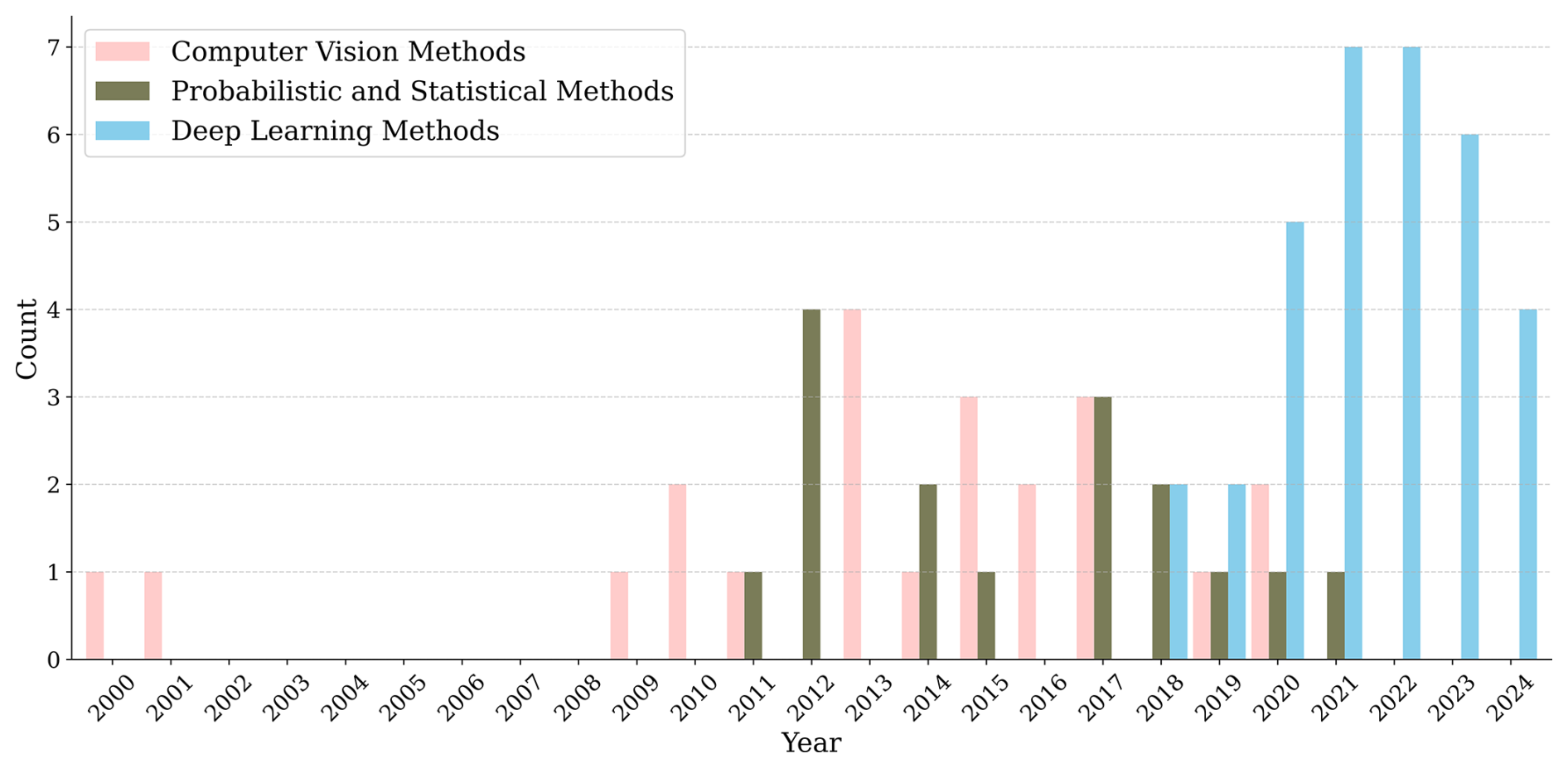
Figure 7 Temporal distribution of research methods: count refers to the number of publications within this field for each year in the respective category (for brevity, again restricted to the time after 2000).

Atefeh Jebeli et al. (2023) aimed at annotating bed and surface horizons using a two-step semi-supervised annotation (TSSA) approach which works on the backbone of ARESELP by Xiong et al. (2017) for producing training data. A U-Net architecture is trained on these data to trace the target boundaries. U-Net is combined with pre-trained VGG19 (Simonyan and Zisserman, 2014) and inception U-Net (Delibasoglu and Cetin, 2020) architectures, also taking advantage of data augmentation to enhance the training outcome. The designed experiments are a combination of the three architectures' augmentation methods. The authors report that U-Net + inception U-Net with data augmentation yields the best results.

To detect depth hoar layers from airborne radar data, Peng et al. (2024) developed a deep learning framework. Their approach includes pre-processing using Fourier transform and wavelet reconstruction for noise reduction. They proposed an improved instance segmentation based on a self-attention mechanism, called ST-SOLOv2. It builds upon SOLOv2 (Wang et al., 2020a) and captures global contextual information. It uses a feature pyramid network (FPN) for multi-scale feature extraction, a dynamic head for classification, and dynamic convolution to decouple the mask branch for better segmentation. The authors used 4230 manually annotated radargrams from NASA OIB snow radar data. The integration of the Swin transformer backbone improves the ability to capture global context and fine-scale details simultaneously. The proposed method shows an improved performance compared with traditional networks such as SOLOv2 (Wang et al., 2020a) and Mask R-CNN (He et al., 2017).

Moqadam et al. (2025) introduced IRHMapNet, a deep learning framework developed for the automatic tracing of IRHs. The framework is based on a U-Net architecture trained on a dataset which is comprised of three groups of data: (i) hand-labeled datasets, in which all the IRHs are manually traced; (ii) IRHs that are the result of image processing methods for tracing IRHs; and (iii) layer slope inference results from the method developed by Sime et al. (2011). The authors employed extensive multi-staged hyperparameter tuning using Bayesian optimization. Apart from the conventional U-Net architecture, Nested U-Net (U-Net$++$) (Zhou et al., 2018) is also used for training. Five experiments were performed, with conventional U-Net performing slightly better than Nested U-Net. Multiple post-processing steps were also performed on the output of the deep learning model, such as thresholding, morphological opening, skeletonization, and connected component analysis. Challenges such as class imbalance and shortcomings of conventional evaluation metrics led to the introduction of a mean vertical distance metric to better measure the alignment between predicted and actual IRHs. The results showed that the proposed method can successfully trace deep IRHs over large spatial extents, achieving continuous and reliable detection.

Table 2 Presentation of published works by either the mapped IRHs or region and the category of methods used. The plus mark signifies the studies that were targeted at mapping more than one group of IRHs.

5 Discussion

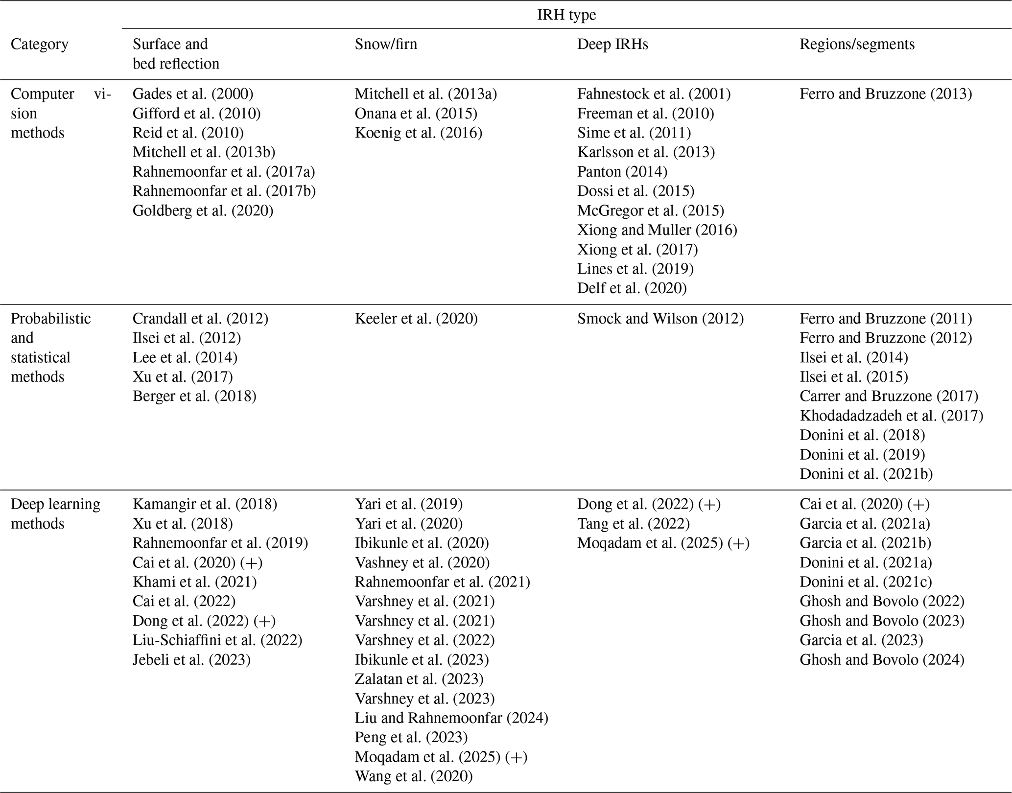
From the timeline of applications to map englacial stratigraphy, we note that methods started off from early-stage computer vision techniques, such as image processing, active contour, Hough transforms, and Radon transforms, and subsequently, a shift occurred towards solutions rooted in probabilistic and statistical approaches, with methods such as HMM emerging as prominent choices. In recent years, the noticeable trend has transitioned towards the adoption of DL techniques. This trend towards the use of deep-learning-based methods is evident from Fig. 7, depicting a categorization of methods that we presented in the previous section. The increasing application of DL techniques across various fields of applications (Minaee et al., 2020; Chen et al., 2022; Sarker, 2021) further emphasizes the likelihood of advancing methods and improving results for radargram segmentation and IRH mapping.

From an application-oriented point of view, there has been a notable transition from methods primarily focused on tracing the air–ice and ice–base boundaries in radargrams (e.g., Gifford et al., 2010; Rahnemoonfar et al., 2017a), mostly for estimating ice thickness and basal roughness, to the increasingly emphasized task of accurately tracing englacial layers. However, most of latter have been employed on layers and horizons in snow and firn and shallower IRHs (e.g., Varshney et al., 2022; Yari et al., 2020) but have been much less often tested on deep IRHs. Table 2 shows a classification of the published work based on both the category of the used methods and the IRH, boundary, or regions that those published works attempted to trace. One of the points that can be clearly noticed in this table is the inadequacy of published models for tracing deep IRHs.

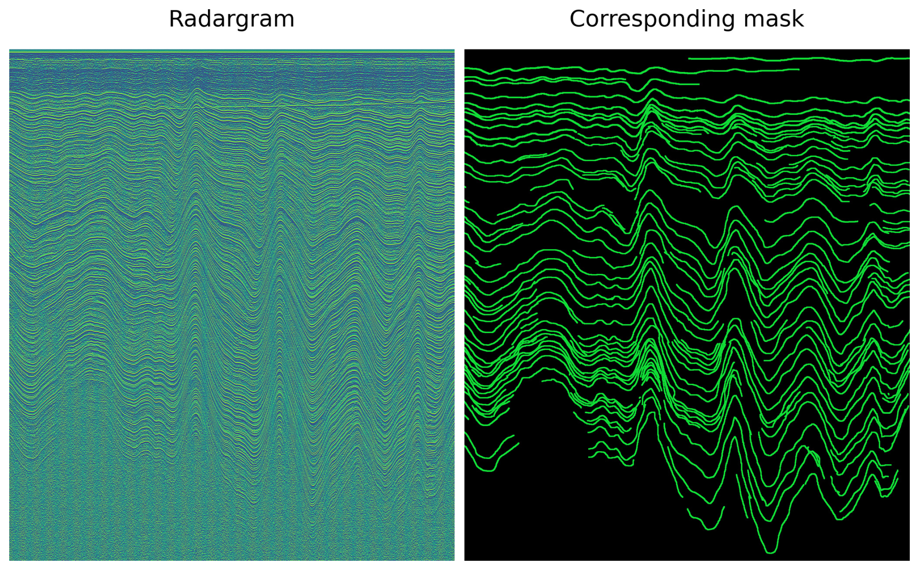
Figure 8 A section of a radargram (Steinhage et al., 2013) and its corresponding entirely annotated mask.

The abundance and closeness of features comprising IRHs in a radargram, often on the order of a couple of wavelengths, along with possible merging and discontinuities of horizons are the main challenges in mapping IRHs. In most other feature extraction and image segmentation applications in glaciology, features and edges (if multiple are present) are usually not located at such short distances from each other as IRHs could be, for example, in glacier grounding-line delineation (Mohajerani et al., 2021). It remains a complex task for any algorithm to detect different features as close as a few pixels from each other and to not merge them when there is no merging to be done but to separately trace them in the case of discontinuities, which are another phenomenon that obstructs mapping attempts (Varshney et al., 2021b). They could emerge as a result of the tracing algorithm's shortcomings and inefficient tracing capabilities. Naturally occurring discontinuities could be due to merging of horizons as a result of decreasing separation of the actual (physical) reflectors at depth, usually below half a wavelength or bandwidth limit, e.g., by compaction for firn layers (Varshney et al., 2021b), ice-dynamic strain thinning (Conway et al., 2002), unconformities caused by changing environmental conditions at the surface (Siegert et al., 2004), heterogeneity of microstructures (Koenig et al., 2016), or simply decreasing surface accumulation along a profile all the way to an erosive regime. Moreover, as the undulation of IRHs in ice sheets becomes more similar to basal topology in the deeper regions, steeper features are more present in deeper parts of the ice sheet (Winter et al., 2019). Such steep features are significantly more challenging to, first, image by RES systems and, second, be differentiated in their structure, even for experts.

The DL approaches which have been applied to mapping and segmenting IRHs are among common architectures and methods that have already demonstrated success in other domains (Choudhary et al., 2022; Emek Soylu et al., 2023; Siddique et al., 2021). However, their inability to yield more satisfactory results in mapping stratigraphy so far can be associated with a number of reasons. One is the aforementioned complexity of radargrams related to the closeness of features and horizons to each other. In many cases, if a method maps an IRH even a few pixels in an incorrect spatial direction, this could be a false prediction and there could be another horizon with a different age at this location. Another possible obstruction for CNN methods is class imbalance, meaning that the number of pixels corresponding to IRHs is far fewer compared to the number of pixels corresponding to the background (non-IRH) class. Unlike tasks such as mapping glacier calving fronts (Mohajerani et al., 2021), in which similar methodologies are applied to images with mostly one boundary in the entire image, radargrams suffer from a much higher level of imbalance between classes. Some solutions have been proposed to overcome this (e.g., Cai et al., 2022; García et al., 2023; Donini et al., 2022a). On the other hand, CNNs are known to be data-hungry and require a large number of annotated data for training (Karimi et al., 2020; Li et al., 2019). Obviously, there seems to be a lack of a large number of annotated data for mapping deep IRHs to be used as training. In most glaciological investigations for which radargrams are annotated, only a handful of IRHs are traced, resulting in a majority of IRHs remaining unlabeled. Such annotations are unproductive for training purposes and confuse the CNN (Tang et al., 2019; Hyun et al., 2020), as some features are traced, while other similar ones are left untraced. In fact, this could have a counter-productive effect for CNN training (Tang et al., 2019). The useful annotations, which would be ideal for training, are radargrams in which all, or at least a large majority, of IRHs are annotated. Figure 8 depicts an example of this.

Even though there have been numerous semi-automatic and automatic attempts to trace surface and basal reflections and a substantial number of attempts regarding snow and firn boundaries, not much work has been done in developing methods which can successfully trace deep IRHs. This lack of methods can be seen in Sect. 4 and Table 1. There are ongoing attempts to map deep reflections along with ongoing efforts to apply machine learning, complemented by transfer approaches, to interpolate and extrapolate layer characteristics across gaps (Bente et al., 2024).

6 Conclusion and outlook

This review aims to provide a contemporary overview of advancements in mapping the internal structure of ice sheets over the past 2 decades. While each of the investigations and developed algorithms presented in this review has contributed to expanding comprehension of mapping the internal structure of ice sheets, the rising incidence of inconclusive and partial results across a number of datasets calls for a thorough and all-encompassing approach for evaluating the methodologies and findings. We assessed the employed methodologies and proposed techniques and outcomes and delineated emerging trends and prospective trajectories for future research.

Due to the vastness of the Antarctic ice sheet, there are still many data that have not yet been adequately or sufficiently analyzed. Moreover, a comprehensive mapped englacial stratigraphy of the Greenland ice sheet, though major stratigraphy is available from manual tracing (MacGregor et al., 2015), and a stratigraphy of mountain glaciers are still points of interest as well. Therefore, the need for a fully automated IRH tracing tool is more than evident. Using such methods, we could increase our knowledge of the age–depth relationship from ice-core sites, which are point measurements, to larger spatial scales and even synchronize age–depth relationships between ice-core sites in much more detail than is currently feasible (e.g., Lilien et al., 2021) and have a complete picture for larger areas between drill sites. An automated method also facilitates imaging regions of past ice-dynamic changes and varying environmental conditions. This would greatly contribute to our understanding of ice sheets' and glaciers' presently visible englacial structure.

We observe that DL-based methods have taken the lead in solving the IRH tracing task in the past couple of years. This can be related to the rapid advances and increasing capabilities that the DL field has been experiencing. Nevertheless, interpreting radargrams poses significant challenges, even for experienced human operators. Radargrams are often noisy and contain a multitude of closely packed features. This complexity arises from their representation over vast depth and length scales, in particular with respect to the radar wavelengths, spanning up to several kilometers vertically and hundreds of kilometers in the flight direction. Consequently, given the broad range of conditions covered by the radar, imaged features and IRHs within radargrams can appear to be discontinuous, merge with each other, or be inadequately represented. These complexities make it difficult for both humans and algorithms to accurately annotate and determine the fate of IRHs and the ice–base boundary. The data acquired by radar systems and the presentation of radargrams have not changed for the past couple of decades. Although system resolution, the signal-to-noise ratio, and signal penetration depth have increased, the visualization of IRHs has not changed considerably. Current research on mapping englacial stratigraphy continues to grapple with the complexity of the task, focusing on fundamental challenges rather than solely refining existing algorithms and methodologies.

The described challenges for automated tracing methods to work properly could be facilitated by establishing a complete pipeline for tracing IRHs, which was trained on a benchmark dataset. Such a dataset would provide the advantage of allowing a more objective, quantifiable, and hence rigorous comparison among different approaches. It has been discussed that performing comparison among different segmentation and edge detection methods would not be a valid comparison since results could depend on the specific criteria of implementation (Kaspersen et al., 2001). Rather, method evaluation on the same dataset would be a valid and quantitative comparison. Since producing datasets such as that shown in Fig. 8 (Moqadam and Eisen, 2024) is quite cumbersome, synthetic datasets that represent the complex features and possibilities of phenomena within radargrams could be the way to go. In addition to complete labeling efforts applied to measured datasets, synthetic approaches can provide progress towards an intermediate solution. There have been a number of synthetic datasets so far (Rahnemoonfar et al., 2019; Dong et al., 2022), but they have not yet been widely considered and used by the community. However, synthetic datasets cannot replace actual radargrams because they lack characteristics of real radar systems such as noise, IRH discontinuities, and merging, to name only a few. Nevertheless, since such obstructions are a matter of resources, it is highly probable that methods capable of automatically tracing IRHs will be developed in the near future.