Toward a marginal Arctic sea ice cover: changes to freezing, melting and dynamics

As the summer Arctic sea ice extent has retreated, the marginal ice zone (MIZ) has been widening. The MIZ is defined as the region of the ice cover that is influenced by waves and for convenience here is defined as the region of the ice cover between sea ice concentrations (SIC) of 15 % to 80 %. The MIZ is projected to become a larger percentage of the summer ice cover, as the Arctic transitions to ice-free summers. Using numerical simulations, we explicitly compare, for the first time, individual processes of ice volume gain and loss in the ice pack (SIC > 80 %) to those in the MIZ to establish and contrast their relative importance and examine how these processes change as the summer MIZ fraction increases over time. We use an atmosphere-forced, physics-rich, sea-ice-mixed layer model based on CICE, that includes a joint prognostic floe size and ice thickness distribution (FSTD) model including brittle fracture and form drag. We demonstrate that this model is realistic using satellite observations of sea ice extent and PIOMAS (the Pan-Arctic Ice Ocean Modeling and Assimilation System) estimates of thickness. A comparable setup has also been compared to floe size distribution (FSD) observations in prior studies. The MIZ fraction of the July sea ice cover, when the MIZ is at its maximum extent, increases by a factor of 2 to 3, from 14 % (20 %) in the 1980s to 46 % (50 %) in the 2010s in NCEP (HadGEM2-ES) atmosphere-forced simulations. In a HadGEM2-ES forced projection, the July sea ice cover is almost entirely MIZ (93 %) in the 2040s. Basal melting accounts for the largest proportion of melt in regions of pack ice and MIZ for all time periods. During the historical period, top melt is the next largest melt term in pack ice, but in the MIZ, top melt and lateral melt are comparable. This is due to a relative increase of lateral melting and a relative reduction of top melting by a factor of 2 in the MIZ compared to the pack ice. The volume fluxes due to dynamic processes decrease due to the reduction in ice volume in both the MIZ and pack ice. For areas of sea ice that transition to being MIZ in summer, we find an earlier melt season: in the region that was pack ice in the 1980s and became MIZ in the 2010s, the peak in the total melt volume flux occurs 20(12) d earlier. This continues in the projection where melting in the region that becomes MIZ in the 2040s shifts 14 d earlier compared to the 2010s. Our analysis shows that a different balance of processes controls the volume budget of the MIZ versus the pack ice. We also find that the balance of processes is different for the MIZ in the 2040s compared to the 1980s, and conclude that we cannot understand the disposition between basal, lateral and top melt in a future Arctic solely based on increased MIZ fraction, since changes in surface energy balance remain a strong control on these behaviours.

1 Introduction

The marginal ice zone (MIZ) is defined as the region of the sea ice cover influenced by ocean waves (Dumont et al., 2011; Horvat et al., 2020). Here, however, we define the MIZ as the region covered by 15 %–80 % sea ice concentration (SIC), which is frequently used due to its easier application (Strong and Rigor, 2013; Aksenov et al., 2017; Cocetta et al., 2024; Strong et al., 2024). The pack ice is then defined as the region where the SIC exceeds 80 %. Whilst the two definitions for the MIZ likely refer to different regions of the sea ice (Horvat et al., 2020), we apply the concentration-based definition in this study since waves are not the critical factor in determining the sea ice mass balance in the Arctic (Bateson et al., 2020; Bateson, 2021). The strength of the sea ice is strongly dependent on the SIC. For 80 % SIC (the upper MIZ boundary), we can estimate that ice strength is less than 2 % of its maximum (Hibler, 1979). In the MIZ, internal stresses in the ice play only a small role and the sea ice is essentially in free drift. The sea ice in the MIZ behaves distinctly to pack ice as it can be more easily advected.

The MIZ grows in early summer as the sea ice cover starts to melt and become more vulnerable to breakup. This leads to an increase in fragmentation, creating a higher fraction of smaller floes. As the sea ice cover shrinks to its minimum extent, the MIZ contracts too. The MIZ forms a much smaller fraction of the sea ice cover throughout the winter months. As the summer Arctic sea ice has retreated over the past 40 years, the fraction of summer sea ice cover that is the MIZ has increased (Rolph et al., 2020). This trend is projected to continue (Strong and Rigor, 2013; Aksenov et al., 2017). This has implications for those wanting to cross the Arctic: a larger Arctic MIZ would be easier to send ships across.

Given the projected increase in the Arctic MIZ fraction, it seems likely that MIZ-focused processes will play an increasing role in controlling the mass budget of the Arctic sea ice. The larger concentration of smaller floes and lower SIC in the MIZ has a number of consequences for the sea ice interactions with the ocean and atmosphere. Lateral melting will be enhanced due to the increased perimeter to surface area ratio (Bateson et al., 2020), creating open water more efficiently than top or basal melt (Smith et al., 2022). The lower the ice concentration, the more the surface ocean is warmed due to the lower albedo of open ocean, further enhancing ice melt and leading to a positive ice–albedo feedback (Curry et al., 1995). The increased open water fraction can also mean an increase in wind mixing in the mixed layer and will affect the Arctic Ocean spin-up (e.g. Martin et al., 2016). Models studying the behaviour of waves in sea ice have identified a positive wave–floe size feedback loop where the smaller the floes, the lower the wave attenuation rate and the further the waves can propagate into the sea ice cover. This then results in further fracture and reductions in floe size (Meylan et al., 2021). There may also be further interesting wave–floe size interactions beyond this, e.g. wave fracture could drive a transition from sea ice acting as a viscous layer to a complete scatterer (Horvat, 2022). The location and volume of sea ice melt has implications for stratification and so how deeply solar heat is mixed down (Peralta-Ferriz and Woodgate, 2015). More sea ice melt means the mixed layer is shoaled and solar heat is concentrated in the upper water column, although the corresponding reduction in SIC and increased sea ice mobility will have a competing effect to reduce ocean stratification via increased input of mechanical energy, e.g. Hordoir et al. (2022). However, there are other important sea ice processes, such as top melting, where it is less clear that we would expect there to be a contrast between the MIZ and the pack ice, e.g. in the formation of melt ponds (Flocco et al., 2012; Rösel and Kaleschke, 2012). In the Arctic, the snow thickness is generally modest compared to that on Antarctic sea ice, and the location of top melting and the initial formation of surface melt ponds is primarily driven by atmospheric conditions, with the subsequent evolution controlled by sea ice topography.

The purpose of a SIC budget is to evaluate the relative contribution of thermodynamic and dynamic processes to the seasonal cycle of ice concentration. The SIC budget from observations has been constructed for the Arctic by Holland and Kimura (2016) using AMSR-E satellite observations spanning 2003–2010. There is no equivalent for ice thickness and volume using observations yet, but a number of studies have assessed the Arctic sea ice mass budget in climate models (Holland et al., 2010; Keen and Blockley, 2018; Keen et al., 2021). Holland et al. (2010) evaluated the mass budget for CMIP3 models over a pan-Arctic scale and found a large amount of variation between the relative importance of processes as the Arctic sea ice declined. The same study also found high model sensitivity both to changes in downwelling longwave and absorbed shortwave radiation and to the initial sea ice state, with thicker initial ice resulting in more sea ice volume change. These findings have implications for efforts to evaluate the sea ice mass budget using model simulations, since they highlight the importance of both ensuring accurate forcing and simulating a realistic time series in sea ice extent and volume.

Following the framework set out by the Sea-Ice Model Intercomparison Project (SIMIP) in Notz et al. (2016) for comparing the energy, mass and freshwater budgets, Keen et al. (2021) compared the sea ice mass balance in CMIP6 models over the 21st century. Although Keen et al. (2021) also found significant differences in the changes to the mass budget component size and timing between the models, they found that when the sea ice state is taken into account, the models behave in a similar fashion to warming, with melting happening earlier in the summer, and growth reducing in autumn and increasing in winter over the coming decades.

In this work, we consider how the processes of ice gain and loss in the MIZ and the pack ice differ, and what this may mean for the future Arctic sea ice cover. Whilst prior studies such as Keen et al. (2021) have evaluated contributions to the sea ice mass balance on a pan-Arctic scale, here we present an analysis of the relative contribution of sea ice processes controlling the mass balance separately for the pack ice and MIZ. We also explore how this may change in the near future in a warming Arctic. This motivates the use of a sea ice model with a higher physical fidelity than used by climate models that is able to capture the distinction of MIZ processes. We use the dynamic-thermodynamic model CICE coupled to a mixed layer model (Petty et al., 2014); the version we use is described in more detail in Sect. 2.1. The model has been used in a number of previous modelling studies, e.g. Schröder et al. (2019), including for comparisons of simulated Arctic MIZ extent against observations (Rolph et al., 2020), and for improving the representation of MIZ processes (Bateson et al., 2020). In order to realistically represent processes in the MIZ, where there is a higher concentration of smaller ice floes, we use a floe size and ice thickness distribution (FSTD) model based on Roach et al. (2018, 2019), that includes brittle fracture (Bateson et al., 2022), found to give realistic simulations of observed floe size distributions (FSD) for mid-range floe sizes in the Arctic (Bateson et al., 2022).

The structure of this paper is as follows. The sea-ice-mixed layer model and atmospheric forcing used is described in Sect. 2.1, observations used to assess the realism of model output are described in Sect. 2.2, followed by a description of the analysis method in Sect. 2.3. Within Sect. 3 of the paper, we first analyse the atmospheric forcing and then compare the simulated sea ice extent and volume against observations in Sect. 3.1. The ice volume fluxes in the pack ice and MIZ in the low MIZ (1980s), high MIZ (2010s) and all MIZ (2040s) scenarios are compared in the next sections. The total annual fluxes are shown in Sect. 3.2, followed by the annual cycle in the main melt and growth terms in Sect. 3.3. We present our Discussion in Sect. 4 and, finally, the main results are summarised in the “Concluding remarks” in Sect. 5.

2 Methodology

2.1 Model setup and forcing

We use a dynamic-thermodynamic sea ice model, CICE, coupled to a prognostic mixed layer model, which is forced by atmospheric reanalysis (detailed in Sect. 2.1) and an ocean climatology. Mixed layer temperature, salinity and depth are all prognostic parameters in the mixed layer model. We used the local CPOM (Centre for Polar Observation and Modelling) version of CICE, which is based on version 5.1.2 (Hunke et al., 2015). This model includes various refinements to the physics, including calibration to CryoSat-2 thickness data (Schröder et al., 2019), the form drag scheme of Tsamados et al. (2014), and a modified version of the joint prognostic FSTD model of Roach et al. (2019), described in Bateson et al. (2022).

We run the model in standalone mode for the pan-Arctic, with a grid resolution of ∼ 40 km. We use the prognostic mixed layer model described in Tsamados et al. (2015), which was adapted for use in the Arctic from the model described in Petty et al. (2014). The mixed layer temperature, salinity and depth are calculated based on heat and salt fluxes from the deeper ocean and the atmosphere/ice at the surface. A restoring is also applied to both mixed layer temperature and salinity towards monthly climatology at 10 m depth, taken from the MyOcean global ocean physical reanalysis product (MYO reanalysis) (Ferry et al., 2011). This restoring is used to capture the moderating effect of ocean currents on mixed layer properties, since the mixed layer model does not allow for interactions between grid cells. The ocean temperature and salinity below the mixed layer are restored to a 3-D ocean grid with winter climatology (for this we take the mean conditions on 1 January from 1993 to 2010) from the MYO reanalysis over a timescale of 3 months. We use a number of the default CICE settings including seven vertical ice layers, one snow layer, thermodynamics of Bitz and Lipscomb (1999), the Maykut and Untersteiner (1971) conductivity, the Rothrock (1975) ridging scheme with a Cf value of 12 (an empirical parameter that accounts for dissipation of frictional energy), the delta-Eddington radiation scheme (Briegleb and Light, 2007), and the linear remapping ice thickness distribution (ITD) approximation (Lipscomb and Hunke, 2004). Additionally, we use a prognostic melt pond model (Flocco et al., 2010, 2012) and an anisotropic plastic rheology (Heorton et al., 2018; Tsamados et al., 2014; Wilchinsky and Feltham, 2006).

The wave forcing data used in this study are prescribed from ERA-Interim reanalysis wave data (Dee et al., 2011) spanning 1979 to 2017. ERA-Interim performs favourably compared to other reanalyses in simulating wind speeds in the Arctic (Jakobson et al., 2012; de Boer et al., 2014). This forcing consists of fields for significant wave height and peak wave period for the ocean surface waves, with these fields updated every 6 h in grid cells that contain less than 1 % sea ice. The approach to determining wave properties within the sea ice applied here is an extrapolation method used previously in Bateson et al. (2022) and described in Roach et al. (2018). This approach differs from Roach et al. (2019), where a separate wave model is coupled to the sea ice model to calculate the wave properties in the grid cells that contain sea ice. The extrapolation method is able to account for discrepancies between the simulated sea ice edge and availability of wave forcing data by searching along lines of longitude to the first ice-free grid cell, where wave properties are defined in the forcing data. Crucially, for this study, despite not having a coupled wave model, our setup still enables wave-induced fracture, causing enhanced lateral melting and wave-dependent new ice formation, as outlined in Roach et al. (2019). Since we only have access to wave forcing data up to and including 2017, for 2018 onwards we repeat the wave forcing data from 2010, which we assessed to be a typical year for wave forcing. There is no trend in the wave forcing thereafter. For the version of the FSTD model used here, Bateson (2021) found limited model sensitivity to a substantial reduction in the attenuation rate of the waves propagating into the sea ice cover by a factor of 10. Whilst several studies have found that the amplitude of waves in the Arctic is likely to increase as the sea ice retreats due to increases in wind speed and fetch – e.g. Casas-Prat and Wang (2020) and Li et al. (2019) – the results presented in Bateson (2021) suggest that the magnitude of the change in wave climate is insufficient to drive major changes in the sea ice state.

We use two atmospheric forcing data sets: NCEP Reanalysis-2 (NCEP2) (Kanamitsu et al., 2002) atmospheric forcing from 1979 to 2020 and HadGEM2-ES (RCP8.5) (Jones et al., 2011) forcing from 1980 to 2050. We use NCEP2 for the hindcast-only simulation since NCEP models generally perform better for near-surface variables compared to other forcing data sets (Jakobson et al., 2012). HadGEM2-ES is one of the Met Office Unified Model climate configurations produced for CMIP5 (Martin et al., 2011). We selected the RCP8.5 pathway since this will produce the maximum possible change in the sea ice state by the end of our study period, best enabling us to explore the implications of a higher MIZ fraction in the future Arctic for the different processes that contribute to sea ice mass balance. Surface air temperature, wind speed and specific humidity are updated every 6 h in the model, incoming shortwave and longwave radiation every 12 h and monthly averages are used for precipitation. Monthly averages are often used for precipitation in atmosphere-forced simulations (Hunke and Bitz, 2009; Tsamados et al., 2015) since there is a high uncertainty associated with precipitation in the reanalysis. The use of monthly averages over higher frequency forcing reduces this uncertainty, although there are limitations to this approach, e.g. it will impact how well resolved the snow to rain transition is within the model. The HadGEM2-ES product is purely model based (no data assimilation) and is included to allow us to consider a projection into the mid-21st century, which enables us to study changes as summer sea ice cover becomes entirely MIZ. We use the first member of the three-member ensemble. HadGEM2-ES has been shown to simulate a realistic Arctic sea ice cover (Wang and Overland, 2012). As we would expect the NCEP data set to be closer to reality due to it being a reanalysis, we treat the NCEP forced simulation as a check and a comparison for the HadGEM2-ES simulation and results in this study. In addition, the use of two different atmospheric forcing data sets allows us to estimate the sensitivity of the results to the forcing used.

Both simulations were initialised with a 6-year spin-up period; this is a similar length to previous studies using the same model setup (Rolph et al., 2020; Bateson et al., 2022). As we are using a standalone sea ice model, the amount of spin-up required is much shorter than a climate simulation, or a coupled sea ice ocean model.

2.2 Observational data

We compare our simulated sea ice extent and MIZ extent with both NASA Team (Cavalieri et al., 1996) and NASA Bootstrap (Comiso, 2017) SIC products. Whilst Rolph et al. (2020) compared a similar model setup to observations, we repeat a similar comparison here since the prior study used an FSTD model without the brittle fracture scheme and only the NCEP reanalysis for atmospheric forcing, not output from HadGEM2-ES. NASA Team has a MIZ extent on the higher end of observational estimates, whilst NASA Bootstrap is on the lower end. The two products give us an estimate of the large range of MIZ extent suggested by satellite products, with this uncertainty resulting from several factors including the presence of melt ponds during summer. Detailed discussions of these two SIC data products and the reasons for differences between them are provided in Comiso (2017) and Kern et al. (2019, 2020). In both cases, the SIC values are interpolated onto the ORCA tripolar 1° grid, which is used by the CICE model. The CICE land mask is applied and the pole hole is filled with 98 % SIC, which is consistent with the surrounding values in the data sets. Daily values are then used to compute monthly values of sea ice and MIZ extent.

PIOMAS, the Pan-Arctic Ice Ocean Modeling and Assimilation System (Zhang and Rothrock, 2003), is a model that assimilates a range of sea ice area/concentration observations to give an estimate of continuous Arctic sea ice volume changes over time. Satellite observations have given us continuous SIC and extent estimates since 1979, but sea ice thickness and volume are more difficult. The presence of snow on the ice introduces substantial uncertainty in ice thickness measurements (Tilling et al., 2018). In addition, satellite thickness products have not historically been produced during summer since both wet snow conditions that emerge during late spring and melt ponds interfere with satellite altimeter retrievals. The continuous nature of the PIOMAS estimates and the pan-Arctic coverage make it a useful comparison for this modelling study, although it should be noted that PIOMAS is known to overestimate the thickness of thinner ice and vice versa for thicker ice (Schweiger et al., 2011). As with the satellite data, PIOMAS has been interpolated on the ORCA tripolar 1° grid and the CICE land mask has been applied.

2.3 Analysis methods

We consider three different ice cover states within the simulations: a low MIZ state in the 1980s; a high MIZ state in the 2010s; and an all MIZ state in the 2040s. Fig. 1 shows the change in MIZ coverage in the summer based on daily July SIC fields from the two simulations plus NASA Team and NASA Bootstrap from the 1980s to the 2010s, and then from the 2010s to the 2040s from the HadGEM2-ES forced simulation. In each case we use the last 5 years of daily July SIC (e.g. 1985–1989 for the 1980s) and assign each grid cell as pack ice (SIC ≥ 80 %), MIZ (15 % ≤ SIC < 80 %) or open water (SIC < 15 %). We then compute where a grid cell spends most of its time in each time period to define each region as pack ice, MIZ or open water. This gives a more accurate representation of where the MIZ is observed and simulated than computing the MIZ from time-averaged SIC fields. We selected a threshold of 80 % for our analysis because it is both a well-established threshold for distinguishing between regions of sea ice in the literature (i.e. the upper limit of the concentration-defined MIZ) and is physically motivated since it approximately corresponds to the transition from ice in free drift to pack ice. In addition, alternative choices for this threshold have practical limitations, e.g. for a higher threshold of 90 %, much of the central pack region will be identified as MIZ due to the opening of leads. For a lower threshold, e.g. 70 %, too few grid cells are identified as part of the MIZ in the 1980s to allow useful analysis. The use of fixed regions for our analysis means that they do not reflect what is MIZ and pack ice on each day of the year. However, it does enable us to analyse volume fluxes (the rate of ice volume loss or gain from a given process) in the region that is predominantly MIZ in July. We use the final 5 years of each decade considered for our analysis to balance the need to capture the transient climatology of a changing system whilst not over-representing extreme events. In addition, this avoids including in the analysis a transition in the early 2010s for the HadGEM2-ES simulation where the model changes from a hindcast to a projection.

Region 1, always pack ice (blue in Fig. 1), is the area that was pack ice in both the 1980s and 2010s (2010s and 2040s); region 2, becomes MIZ (green), is the area that was pack ice in the 1980s (2010s) and became MIZ in the 2010s (2040s); and region 3, always MIZ (orange), is the region that was MIZ in both the 1980s and 2010s (2010s and 2040s).

We analyse the simulated annual volume fluxes in Sect. 3.2 and annual cycles for the melt terms and congelation growth in Sect. 3.3 using the regions defined in Fig. 1 over the 5-year study periods as described previously. The terms of the sea ice volume budget we examine in each simulation for each region and time period are as follows:

• congelation growth – basal thickening of the sea ice;

• frazil ice formation – supercooled seawater freezing to form frazil crystals which clump together to create sea ice;

• snow ice – snow ice formed when the ice–snow interface on top of the sea ice is pushed below water, resulting in the flooding and freezing of snow;

• basal melting – melting at the base of the sea ice;

• top melting – melting on the surface of the sea ice;

• lateral melting – melting at the edge of the sea ice floes;

• sublimation – sublimation from the surface of the sea ice, both ice and snow sublimation output included in this model output;

• dynamics – the net import or export of sea ice within a given domain resulting from advection and convergence/divergence.

These terms collectively account for all sources and sinks of sea ice volume captured by our model setup within a given region.

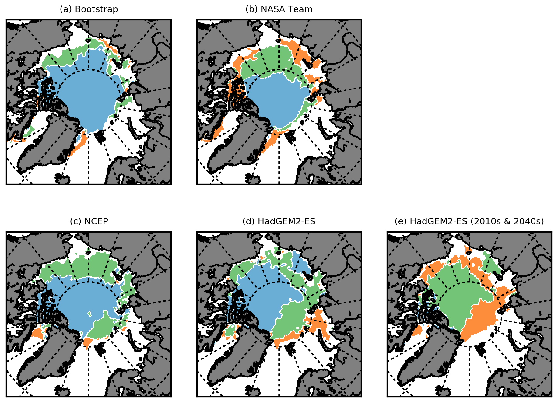
Figure 1 Regions of the Arctic sea ice cover defined from daily July ice concentration fields from each time period from the NCEP and HadGEM2-ES forced simulations. Each time period refers to the final 5 years of the referred to decade, e.g. 1980s refers to the average behaviour over 1985–1989. Region 1 (blue) indicates the area that is pack ice in both the 1980s (2010s) and 2010s (2040s) in (a)–(e). Region 2 (green) indicates the area that is pack ice in the 1980s (2010s) and becomes MIZ in the 2010s (2040s) in (a)–(e). Region 3 (orange) indicates the area that is MIZ in both the 1980s (2010s) and the 2010s (2040s) in (a)–(e).

3 Results

3.1 Comparison of model output to observations

The surface air temperatures are significantly higher in the NCEP reanalysis than HadGEM2-ES between December to early April in both the 1980s and 2010s period, as shown in Fig. 2a. For the rest of the year they are more comparable, apart from the HadGEM2-ES forcing being slightly warmer in October and November. The largest warming is seen from September through the autumn. Looking at the change in annual average values in Fig. 3 we can see that between the 1980s and 2010s, both NCEP and HadGEM2-ES warm by roughly 2 °C across the central Arctic. The warming continues at a similar pace in the HadGEM2-ES to the 2040s, with warming of typically 8 °C across the central Arctic from the 1980s, including near the Canadian archipelago, where warming is slightly lower in the 2010s. The humidity values shown in Fig. 2b are relatively similar in the NCEP and HadGEM2-ES forcing sets, with higher humidity values in the NCEP forcing set during the December–early April period. In both data sets, the humidity increases over time in all months, particularly from July through until December. The shortwave and longwave radiation values are very different between the two data sets, as shown in Fig. 2c and d. NCEP has much higher summer shortwave radiation values, whilst HadGEM2-ES has much higher year-round longwave radiation values, particularly during summer. It is likely that this dramatic change is due to differences in cloud cover (Holland et al., 2010; Zib et al., 2012). Consistently higher wind speeds throughout the year are also found for the NCEP atmospheric forcing compared to HadGEM2-ES, although both forcing data sets display high daily variability. No clear change in wind speeds can be seen for either forcing data set from the 1980s to the 2010s (or from the 2010s to the 2040s for the HadGEM2-ES forcing).

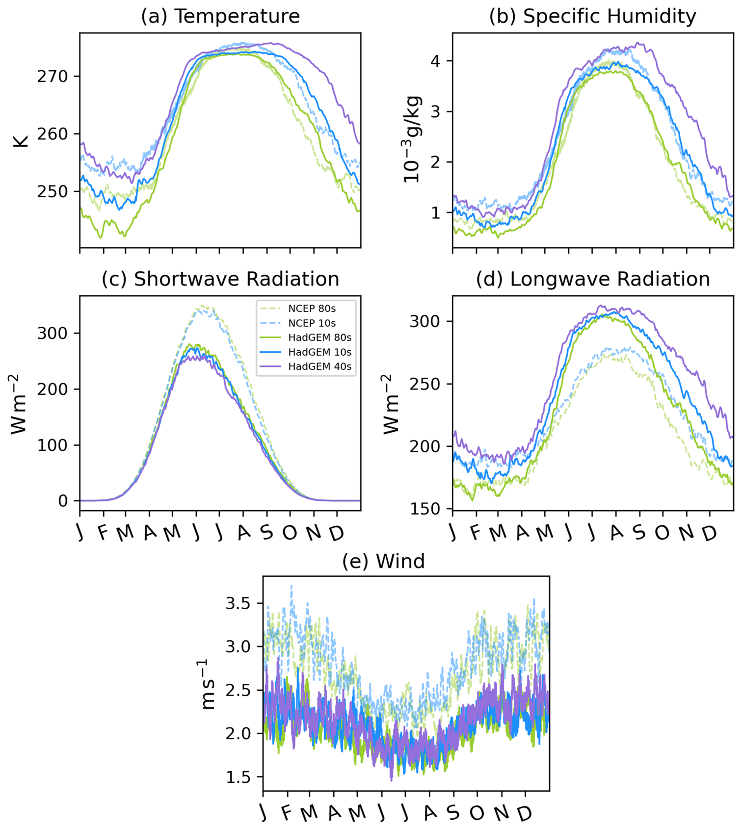
Figure 2 NCEP and HadGEM2-ES atmospheric forcing, (a) surface air temperature, (b) specific humidity, (c) shortwave radiation, (d) longwave radiation, and (e) wind speed are shown for the 5-year study periods during the 1980s, 2010s and 2040s, as outlined in Sect. 2.3, over the ocean north of 66.5° N.

Figure 3 NCEP and HadGEM2-ES warming between the 5-year study periods. (a) 2010s–1980s (NCEP), (b) 2010s–1980s (HadGEM2-ES) and (c) 2040s–1980s (HadGEM2-ES). The differences are between the annual average near-surface air temperatures. Averages are taken over the final 5 years of each decade, e.g. 1980s refers to the average behaviour over 1985–1989.

There is a large range in the MIZ coverage estimated by satellite products (Rolph et al., 2020). We choose NASA Bootstrap and NASA Team for this comparison to give an indication of lower and upper observational estimates of MIZ extent. NASA Team has a much larger region that becomes MIZ and is always MIZ than Bootstrap. The MIZ coverage in the NCEP and HadGEM2-ES forced simulations is closer to Bootstrap in the 1980s and closer to NASA Team in the 2010s, as given in Fig. 4. Considering both Figs. 1 and 4, the simulations show both a different spatial distribution in the MIZ and changes to the MIZ coverage compared to the satellite observations. The simulations show a larger increase in the MIZ north of Svalbard, particularly in the HadGEM2-ES forced simulation. There is a similar change in the percentage of MIZ coverage in the two simulations, with the HadGEM2-ES forced simulation showing slightly more MIZ in both periods. By the 2010s the MIZ makes up 46 % and 50 % of the July sea ice cover in the NCEP and HadGEM2-ES forced simulations, respectively, and 93 % by the 2040s in the HadGEM2-ES forced projection (see Fig. 4).

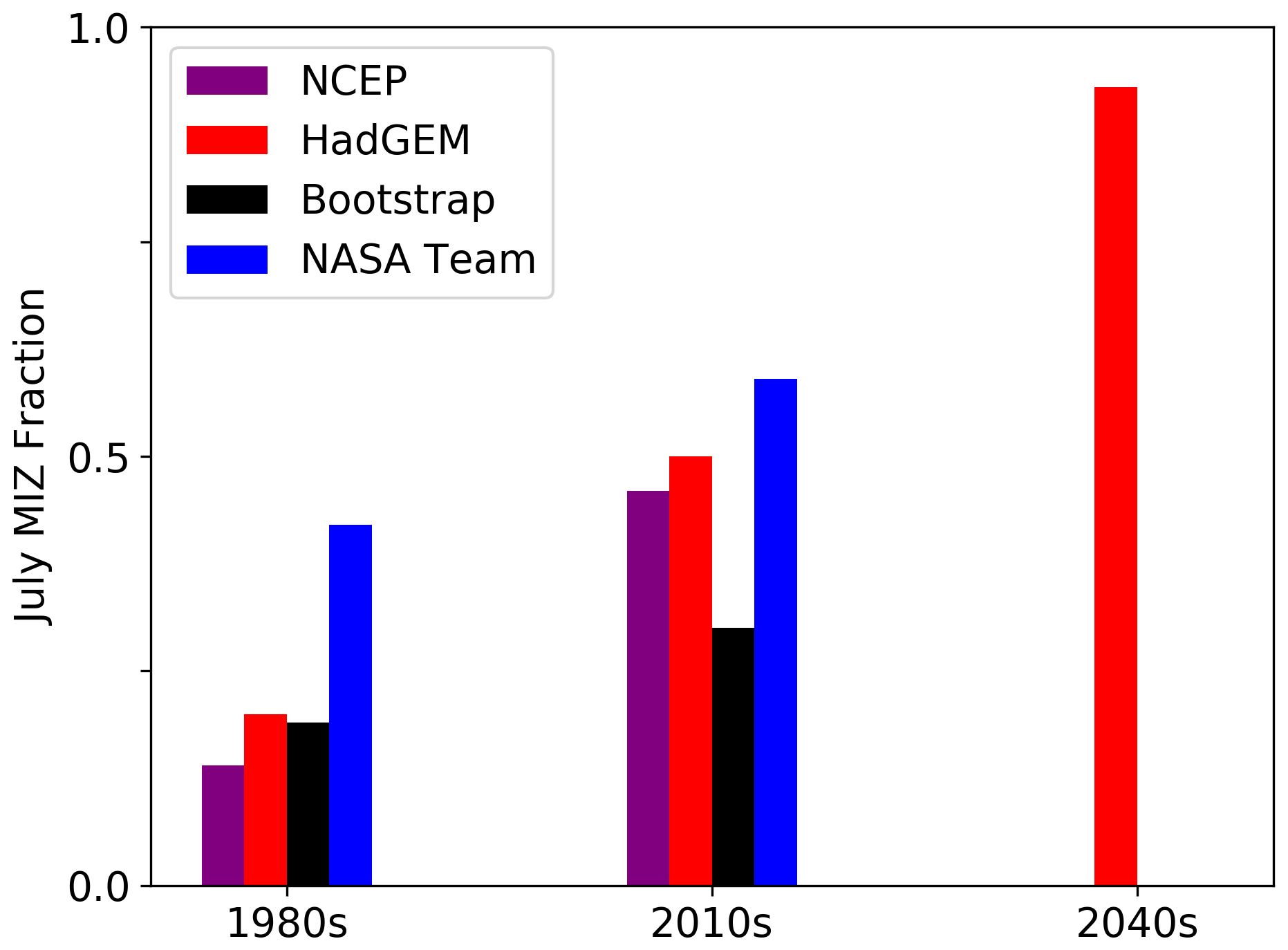
Figure 4 Fraction of the July sea ice cover that is MIZ in each 5-year study period from the two forced CICE simulations and satellite observations from NASA Team and NASA Bootstrap (see Sect. 2.2).

The NCEP forced simulation spans from 1979 to 2020, whilst the HadGEM2-ES simulation spans from 1980 to 2050. The monthly sea ice and MIZ extent values for June, July, August and September are given in Fig. 5, alongside values from NASA Team and Bootstrap. In Fig. 6, averaged annual time series in both sea ice and MIZ extent for the 1980s and 2010s are presented for the simulations and observations. These figures show that the total sea ice extent values in the atmosphere-forced simulations are in relatively good agreement with NASA Team and NASA Bootstrap in the summer months, showing slightly lower minima. The simulations show a weaker negative trend in total sea ice extent in June and July (Fig. 5a, b), whilst being slightly lower, but very similar to the satellite observations in August and September (Fig. 5c, d). Both simulations overestimate winter sea ice extent compared to satellite observations, with this bias increasing in the 2010s due to the larger drop in winter sea ice extent in the satellite observations from the 1980s to the 2010s.

Fig. 5 shows that whilst the total sea ice extent observations are generally in good agreement, satellite observations show a large range of estimates for the MIZ (see also Rolph et al., 2020). The interannual variability in the MIZ extent in both simulations and observations in July, August and September (Fig. 5b, c, d) is large, albeit smaller for the Bootstrap data set than NASA Team. Figs. 5 and 6 both show a lack of trend in MIZ extent for NASA Team and Bootstrap in any month, though because of the decreasing trend in summer sea ice extent, the fraction of the sea ice cover that is MIZ increases. The simulations show an increasing trend in MIZ extent for July and August (albeit stronger for NCEP), starting off close to the Bootstrap MIZ extent values in the 1980s, and ending up closer to the NASA Team values in the 2010s. For July, this transition primarily emerges from 2000 onwards. In the 2010s, the MIZ has generally become the dominant part of the sea ice cover in July, August and September for both the simulations and the NASA Team data set. In comparison, for the Bootstrap data set, the MIZ fraction is mostly below 50 % of the total sea ice cover. For the HadGEM2-ES forced simulation, by the end of the 2030s, the sea ice cover has become almost entirely MIZ in August and September, and in the 2040s, the sea ice extent in August and September goes below the value commonly used to define the Arctic as ice free (1×10⁶ km²).

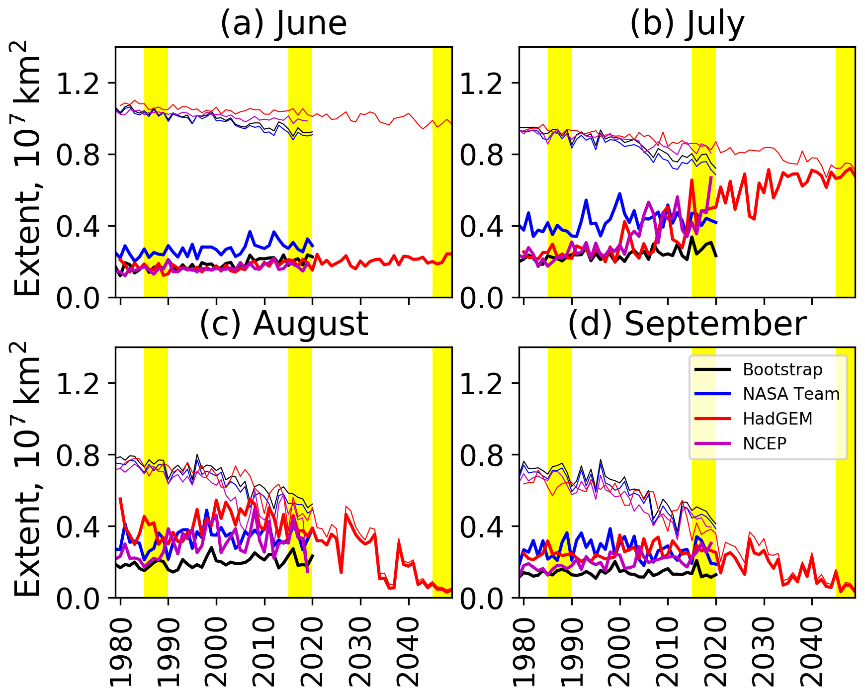
Figure 5 Monthly June, July, August and September sea ice (thin lines) and MIZ extent (thick lines) from the NCEP (1979–2020) and HadGEM2-ES (1980–2050) forced simulations compared to satellite observations from NASA Team (1979–2020) and NASA Bootstrap (1979–2020). Yellow shaded areas show the three 5-year study periods used (see Sect. 2.3).

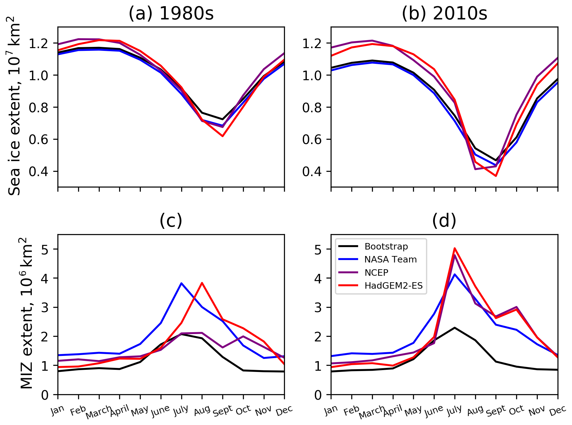
Figure 6 Monthly values of sea ice extent and MIZ extent over 1985–1989 and 2015–2019 for the NCEP and HadGEM2-ES forced simulations and satellite observations from NASA Team and NASA Bootstrap.

In Fig. 7, we compare the total sea ice volume over the Arctic Ocean from the HadGEM2-ES and NCEP forced simulations, alongside monthly values from PIOMAS. In Fig. 7a, we can see that the NCEP forced simulation overestimates the seasonal cycle, mostly due to too much sea ice volume in the winter, but is nonetheless relatively similar to the PIOMAS estimate (difference plot in Fig. 7b), showing similar variability. Meanwhile, the HadGEM2-ES forced simulation underestimates the sea ice volume all year round (Fig. 7a), although it does tend towards to the PIOMAS estimate over time (Fig. 7b) due to showing a smaller sea ice volume decrease over time. Both simulations produce suitably realistic sea ice extent and volume for the scope of this study.

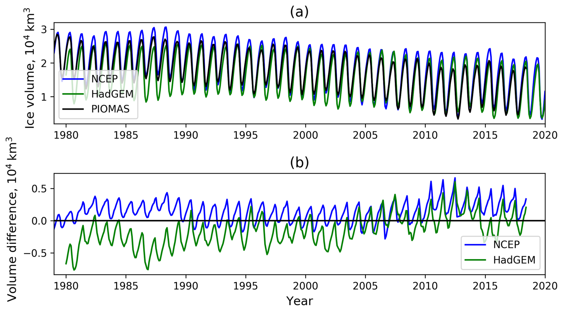
Figure 7 Monthly Arctic sea ice volume from NCEP and HadGEM2-ES forced simulations compared to PIOMAS in (a) and the differences from PIOMAS shown in (b).

3.2 Total annual volume fluxes

In order to explore changes in the sea ice mass budget over time and how this differs between the different regions, Fig. 8 presents the cumulative annual fluxes for the different sea ice processes. Fig. 9 then shows the fractional contribution of different sea ice loss processes to the total sea ice loss. Fig. 8 shows that in all regions and in both simulations, basal melt makes up the largest proportion of melting (except for always pack ice in the HadGEM2-ES case, where top melting is slightly higher in magnitude). We also see an increase in annual basal melt flux moving from the always pack ice region to the always MIZ region for each case. In the 1980s and 2010s, top melting is substantially more important in the pack ice than in the MIZ. Fig. 9 shows that top melt makes up roughly twice as much of the melting in the region of always pack ice compared to the region of always MIZ. The opposite is true for lateral melting – the fraction for lateral melting in regions of always MIZ is more than twice the fraction in regions of always pack ice. This makes the fraction of top and lateral melt comparable in the always MIZ region, particularly in the NCEP simulation. Overall, Fig. 9 shows that the partitioning of the melt between top, basal and lateral melting differs substantially between the pack ice and MIZ. For the always pack ice region, both top and basal melt contributions to total sea ice loss are in the range 25 %–50 % across the 1980s and 2010s for both simulations, whereas in the always MIZ region, the basal melt contribution to total sea ice loss exceeds 60 %, with the top melt contribution around or below 20 %. This partitioning is broadly consistent between the two forced simulations over the 1980s and 2010s.

We can also identify clear differences in how the different regions change from the 1980s to the 2010s. Fig. 8a shows that for the NCEP forced simulation we see the basal and lateral melt fluxes approximately double from the 1980s to 2010s for the always pack ice region. We also see an increase of over a third in the top melt flux. In Fig. 9a, we see that the net effect of this change is an increase in the melt contribution to sea ice loss in the always pack ice region from about 70 % to 85 %, reducing the contribution of dynamics by about a half. The changes for the HadGEM2-ES case for the same period are qualitatively the same, though the magnitude of the change is smaller. There is also a change in partitioning in the melt components from the 1980s to the 2010s for the always pack ice region; e.g. Fig. 9d shows a decrease in the fraction lost to top melt for the HadGEM2-ES forced simulation, with a corresponding increase in the fraction lost to lateral and basal melt. Overall, this indicates a tendency towards the values seen in the becomes MIZ region. In comparison, Fig. 8 shows that for the always MIZ region we see very little change in the lateral melt annual volume flux from the 1980s to the 2010s, but we do see small reductions (of the order 5 %–10 %) in the top and basal melt annual volume flux. In this region, there will be competing effects of the reduced SIC versus increases in melt rate due to changes in surface energy balance. For the lateral melt rate, reductions in the average floe size will also have an impact. In Fig. 9, we see only small changes in repartitioning between the melt components but a net increase overall in the melt contribution to sea ice loss. By the 2010s, the contribution of dynamics to sea ice loss is just a couple of percent in the always MIZ region.

It is surprising that there is not a more significant change in the becomes MIZ region from the 1980s to the 2010s in terms of the proportion of melt that is top, basal or lateral (see Fig. 9). It might have been expected that the balance would have shifted between the two time periods. Instead, the values are approximately midway between those of the always pack ice and always MIZ regions. The ratio of lateral to basal melt for a given floe is inversely proportional to floe size, so a lack of change in this ratio suggests limited changes in average floe size within the becomes MIZ region. This may partly be a result of how processes that drive the fragmentation of sea ice over the transition from pack ice to MIZ, in particular in-plane brittle failure, are currently represented in the FSTD model (Bateson et al., 2022). Overall, the lack of change in the proportion of melt that is top, basal or lateral within the becomes MIZ region over time shows that these melt ratios cannot be considered solely as a function of SIC.

Dynamics (advection and convergence/divergence) results in a net negative flux in all regions, though the magnitude is significantly larger in the pack ice than in the MIZ, as might be expected due to a larger volume of sea ice that can be advected. These results reflect that generally sea ice is exported outwards from the central Arctic and melts at lower latitudes. This means that dynamics plays a more significant role in ice loss in the always pack ice region compared to the becomes MIZ and always MIZ regions. In all regions, there is a strong decrease in the proportion of ice loss that is due to dynamics from the 1980s to the 2010s, with the largest change occurring in the NCEP always pack ice region. This change will at least partly be a result of reduced sea ice thickness, particularly given the lack of trends in wind speed shown by Fig. 2. Dynamics is comparable to lateral melting in the becomes MIZ region, much larger in the always pack ice region and smaller in the always MIZ region. Whilst Fig. 2 shows that the NCEP forcing has higher wind speeds compared to the HadGEM2-ES forcing, a larger dynamics contribution to sea ice volume loss for the NCEP forced simulation compared to the Hadgem2-ES forced simulation can only be found in the always pack ice region, particularly in the 1980s, with only small differences found for the other regions.

Figure 8 shows that congelation growth dominates sea ice growth, making up 91 %–95 % in both the pack ice and MIZ regions. Frazil is the next biggest ice growth term, making up 5 %–9 %. In all cases, snow ice formation is a negligible contribution to sea ice growth, making up less than 1 % in all periods and regions. This growth partitioning applies to both the NCEP and HadGEM2-ES forced simulation; there are some small changes over time in each region, as shown in Fig. 8, but not outside the range stated previously. We do see an increase in growth terms in the always pack ice region from the 1980s to the 2010s (particularly for the NCEP case), though this is as expected given that higher growth rates are expected for thinner ice due to a faster rate of conduction.

For the HadGEM-ES forced projection, panels (g) and (h) in Fig. 8 show a small increase in overall melt in the becomes MIZ region and a reduction in all three melt terms in the always MIZ region from the 2010s to the 2040s. Fig. 9 shows that the fractional contribution of basal and particularly top melt to sea ice volume loss increases across both regions, with a small reduction in the lateral melt contribution and a larger reduction in volume loss due to dynamics. This result is consistent with the increased role for top melting seen in the near future in CMIP6 model projections (Keen et al., 2021). This is likely driven by the increase seen in the surface air temperature and downwelling longwave radiation in the atmospheric forcing, as shown in Figs. 2 and 3. Fig. 8 shows a reduction in congelation growth across both the becomes MIZ and always MIZ regions, though the changes in frazil ice growth are either negligible or positive. The former can be explained due to the overall warming in the Arctic system reducing overall sea ice growth in the 2040s, whereas the latter is consistent with there being larger regions of open ocean during periods of sea ice formation. The top, basal and lateral melt fractions in the projection to the 2040s do not match the earlier period for the corresponding region in the HadGEM2-ES forced simulation. It is notable that the melt partitioning shown in panel (g) in Fig. 9 for the becomes MIZ region both in the 2010s and 2040s looks like the partitioning seen for the always pack ice region in panels (a) and (d). Similarly, the always MIZ region shown in panel (h) has a similar melt partitioning to the becomes MIZ region shown in panels (b) and (e). More generally, whilst there are changes in sea ice behaviour as it transitions from pack ice to MIZ, these changes are smaller than expected given the differences in the melt partitioning between pack ice and MIZ shown by Figs. 8 and 9. The location (e.g. latitude) of the sea ice also appears to be important in determining the balance of processes.

3.3 Annual cycle of melt and growth

To better understand the net changes in annual sea ice volume fluxes and investigate changes to the onset and length of melting, we looked at the average annual cycle of congelation growth, basal, top and lateral melt fluxes, shown in Fig. 10. The same regions and time periods defined in Fig. 1 have been used.

Melting occurs first in the outer regions (always MIZ regions) and progresses inwards across the sea ice cover to the always pack ice region. This is more pronounced in the NCEP simulation, which is likely a reflection that the NCEP atmospheric forcing is warmer in summer (see Fig. 2a). The peak in top melting occurs first, followed by the peak in basal melting in the always pack ice and becomes MIZ regions. Lateral melting has a less pronounced summer peak that appears later in the melt season (early August) than the other melt terms, reflecting the increase in fragmentation of the sea ice cover as the summer progresses. Lateral melting is a larger melt term in the MIZ regions, as noted in the previous section. The total melt and growth rate (per unit area) is larger in the MIZ than the pack ice in the 1980s in both simulations; this difference decreases in the 2010s as melting and growth fluxes increase in the always pack ice region by more than in the becomes MIZ and always MIZ regions, reflecting the increase in seasonality in the pack ice.

In order to characterise the changes in the annual cycle of sea ice melt and growth shown in Fig. 10, we consider the change in onset of melt, end of melt and onset of growth from the 1980s (2010s) to the 2010s (2040s), expressed in days. To determine these metrics, we use a threshold of $\mathrm{2.5}\times {\mathrm{10}}^{-\mathrm{3}}$ m³ m⁻² d⁻¹ applied to total melt and growth. We select this threshold to capture the main phases of melt and growth, as opposed to oscillations or lower rates of melting. We also consider the change in the timing of peak total melt volume flux (hereafter referred to as peak melt rate) and the percentage increase in the peak melt rate from the 1980s (2010s) to the 2010s (2040s).

In the always pack ice region, peak melt rate increases and the melt season gets longer in the 2010s relative to the 1980s by 13 d in the NCEP and 6 d in the HadGEM2-ES forced simulations. This is primarily due to earlier melting onset by 9 d in the NCEP and 8 d in the HadGEM2-ES forced simulation. Peak melting rates increase, particularly in the NCEP simulation, where they increase by 49 %, compared to a 17 % increase in the peak melting rate in the HadGEM2-ES simulation. The increase in total melt rate across the melt season for both cases will be driven by changes to the surface energy balance. In particular, Fig. 2 shows that there is an increase in mean atmospheric surface temperature and downwelling longwave radiation for both reanalyses, though this effect will be partly compensated by the small reduction in downwelling shortwave radiation. There are larger increases in surface temperature and longwave radiation for NCEP than HadGEM2-ES over July to August, i.e. the period of peak melting, likely explaining the higher percentage change for the former. The increase in total melting is one factor that drives a larger seasonal sea ice cycle (see Fig. 7a). The second major contributing factor is the increase in sea ice growth rates shown in Fig. 10, since sea ice growth rates are higher for thinner ice. This increase is particularly large in the NCEP simulation, where congelation growth increases by 74 % on average over October, November and December. The average increase in basal growth rates in the HadGEM2-ES forced simulation is much lower, at 17 %.

In the becomes MIZ region, the increase in peak rate of melting is again larger in the NCEP simulation, but not as dramatic as in the always pack ice region. Peak total melting rates increase by 29 % in the NCEP and 13 % in the HadGEM2-ES forced simulation and there is a shift in the melting season in the 2010s relative to the 1980s. The start of melting shifts earlier by 9 d in the NCEP and 5 d in the HadGEM2-ES forced simulation, whilst the end of summer melting ends earlier by 16 d in the NCEP and 14 d in the HadGEM2-ES forced simulation, overall shortening the period of melting despite the earlier onset. Peak melting occurs much earlier, by 20 d in the NCEP and 12 d in the HadGEM2-ES forced simulation. The earlier timing in the peak melt rate is driven by reduced sea ice mass balance within the becomes MIZ region (e.g. a lower SIC will result in reduced top and basal melt fluxes). The earlier timing in the end of summer melting is a result of the melt out of sea ice in this region during summer in the 2010s. In both simulations, we see lower growth rates in late September and early October in the 2010s compared to the 1980s, but in both cases we see a transition where the 2010s growth rate becomes higher (late October for NCEP and early December for HadGEM2-ES). In December, we see a larger increase for the NCEP simulation. The delayed freeze-up is primarily driven by changes in the surface energy balance (e.g. higher atmospheric surface temperatures) and an increase in heat accumulated over the prior melt season within the ocean surface mixed layer. The higher growth rates later in the year are a result of the inverse relationship between growth rate and ice thickness.

In the always MIZ region, the changes in the annual cycle for melting processes from the 1980s to the 2010s are much smaller compared to the other regions. The peaks in melting stay a similar magnitude and occur at a similar time, only a few days earlier in both simulations. Melting onset shifts slightly earlier, by 6 d in the NCEP and 5 d in the HadGEM2-ES simulation. In the HadGEM2-ES simulation, there is a significant shift earlier in the end of melting by 19 d (just 4 d earlier in the NCEP simulation). This suggests a complete or almost complete melt out of sea ice in this region. Growth rates in both simulations decrease over the October–December period, with the NCEP average decreasing by 16 % and the HadGEM2-ES average decreasing by 20 %. There is very little to no sea ice across this region by the end of the melt season in both the 1980s and 2010s, and therefore changes in this region are not driven by the relationship between ice thickness and growth rates. Other factors such as the ocean heat content and atmospheric surface temperatures are the primary drivers behind any differences in growth rates.

In the projection, moving from the 2010s to the 2040s, we see the same trends in the becomes MIZ and always MIZ regions, as seen in the 1980s to 2010s comparison. The start of melting shifts earlier by 7 d in both the becomes MIZ and always MIZ regions. The melt season shrinks, mostly due to the large shift of the end of the melt season, by 20 d in the becomes MIZ region and 21 d in the always MIZ region. This reflects all of the ice in those regions having melted. This is combined with a later start to congelation growth in the autumn by 9 d in the becomes MIZ region and 21 d in the always MIZ region, followed by slower growth rates in both regions – 17 % and 37 % slower in the becomes MIZ and always MIZ regions, respectively, over October, November and December. For the becomes MIZ region, it might be expected that the average rate of congelation growth would increase from the 2010s to 2040s over October to December due to the reduced mean ice thickness. However, in this case, the changes that act to reduce congelation growth, e.g. the increase in longwave radiation and surface air temperature over the autumn and winter months shown by Fig. 2, have a larger impact.

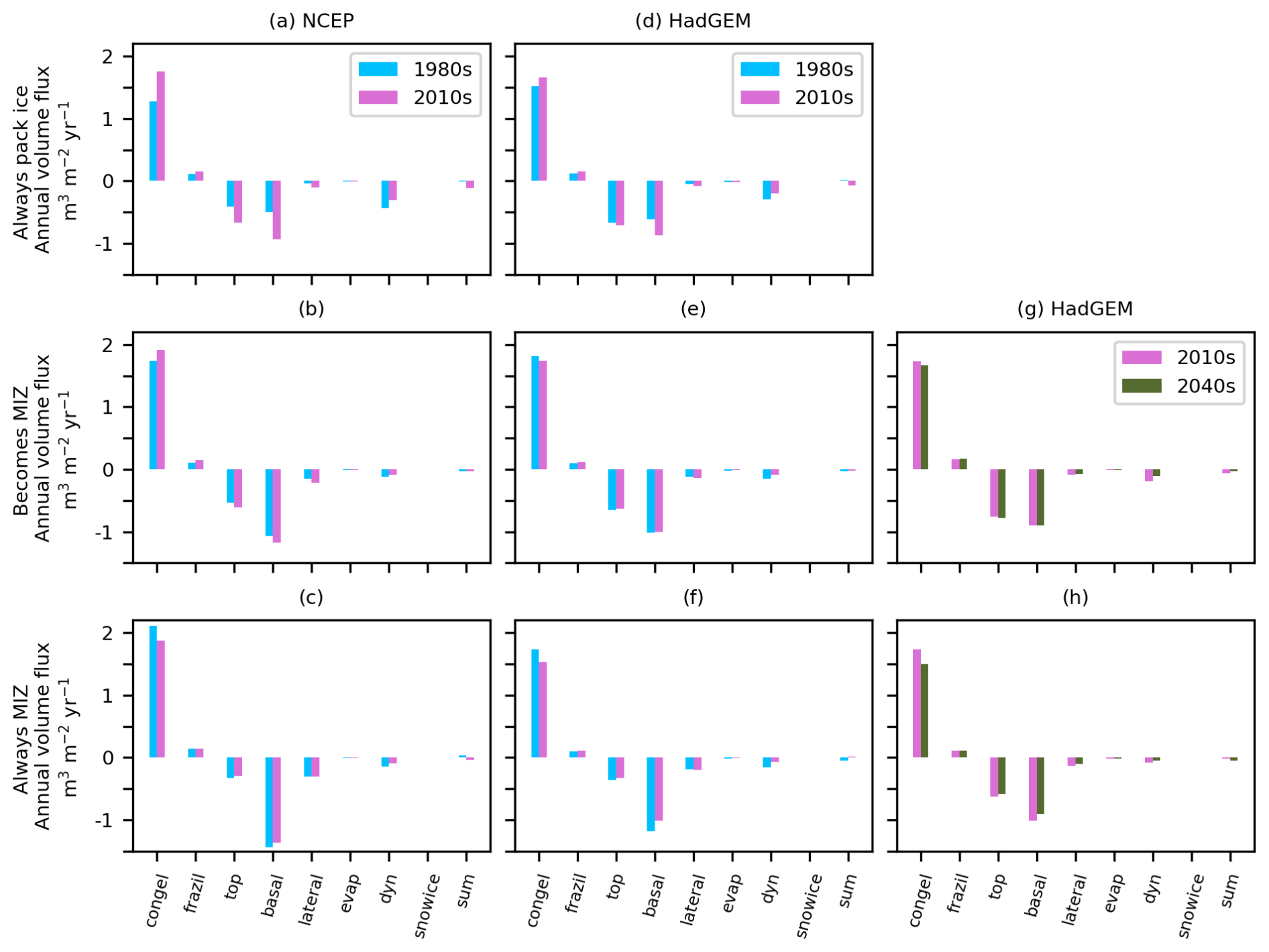
Figure 8 The total annual volume fluxes of sea ice over regions shown in Fig. 1 for congelation ice growth, frazil ice formation, top melt, basal melt, lateral melt, sublimation, dynamics (advection and convergence/divergence), snow ice formation and the sum of all the terms. The summed annual volume fluxes are calculated from the average annual cycle over the 5-year study periods during the 1980s, 2010s and 2040s, as outlined in Sect. 2.3. Subplots (a)–(c), (d)–(f) and (g)–(h) use the regions shown in Fig. 1c, d and e, respectively.

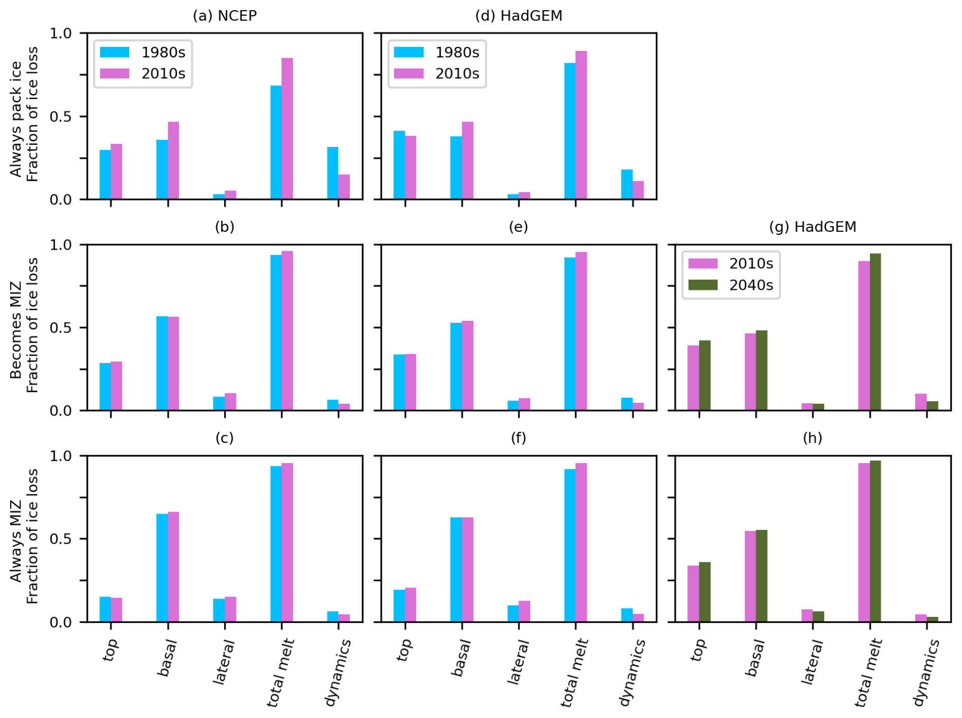
Figure 9 The amount of ice loss due to top melt, basal melt, lateral melt, total melt (the sum of the three individual melt terms) and dynamics (advection and convergence/divergence), expressed as a fraction of the total of the sum of these terms. Note that the evaporation term is neglected in this analysis. Results are presented for regions shown in Fig. 1 over the 5-year study periods during the 1980s, 2010s and 2040s, as outlined in Sect. 2.3. Subplots (a)–(c), (d)–(f) and (g)–(h) use the regions shown in Fig. 1c, d and e, respectively.

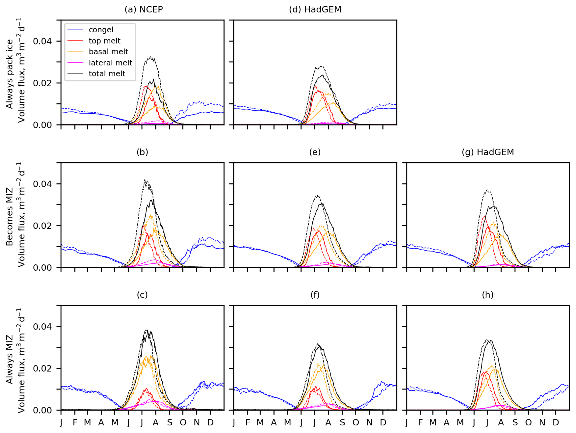
Figure 10 The time-averaged annual cycles of congelation ice growth, top melt, basal melt and lateral melt in the regions described in Fig. 1. The solid lines show the 1980s average in subplots (a)–(f) and the 2010s in subplots (g)–(h). The dashed lines show the 2010s average in the subplots (a)–(f) and the 2040s in subplots (g)–(h). Subplots (a)–(c), (d)–(f) and (g)–(h) use the regions shown in Fig. 1c, d and e, respectively.

4 Discussion

In this study, we chose to run simulations with both the NCEP and HadGEM2-ES forcing so that the NCEP forced simulation could act as a check on the HadGEM2-ES forced simulation, which is projected to 2050. The two simulations were relatively similar in terms of sea ice extent, MIZ extent (see Sect. 3.1) and MIZ fraction (see Fig. 4). We compared key extent and volume metrics from both simulations to observations to demonstrate that they simulate a reasonable sea ice state, which has been shown to affect the balance of sea ice processes (Holland et al., 2010; Keen et al., 2021). The overall results and proportions of growth and melt were largely similar in the two simulations. However, the changes between the 1980s to the 2010s were generally larger in the NCEP forced simulation. This includes the changes in volume fluxes in both regions (see Fig. 8a–f), reflecting the larger reduction in summer sea ice volume between the two periods (see Fig. 7a). The differences between the NCEP and HadGEM2-ES forced simulation volume changes are largely a reflection of HadGEM2-ES having a much lower sea ice volume in the 1980s. However, as the simulations become closer over time, it is possible that the HadGEM2-ES simulation might underestimate the change from the 2010s to the 2040s.

A key motivation for this study was to better understand the impact of an increasing MIZ fraction on the sea ice mass balance budget both for the present-day and future Arctic (Rolph et al., 2020). Our results show that sea ice volume fluxes do have some dependence on ice concentration, as would be expected, e.g. Fig. 9 consistently shows a larger role for lateral melt and a reduced role for top melt in the MIZ compared to pack ice. We also see different changes over time in these regions. In particular, Fig. 10 shows that from the 1980s to 2010s, we see substantial changes in the seasonal cycle in total melt in both the always pack ice and becomes MIZ regions, with the melt season shifting both earlier and with a stronger peak. In comparison, changes in the always MIZ region are much smaller. This reflects the transition of the Arctic sea ice cover overall to a more seasonal state, where there is an increasing importance of the inner MIZ and even the pack ice in contributing to seasonal sea ice loss via melting. However, the analysis used here has also demonstrated that SIC is not the only metric that determines the balance of processes that contribute to the sea ice mass balance. Fig. 9 shows that the melt partitioning between the top, basal and lateral melt processes within the MIZ in the 2040s looks closer to the partitioning shown for the pack ice in the 1980s rather than the MIZ. This suggests that physical location of the sea ice is also a key control on this partitioning, which is primarily a proxy for surface energy balance.

For this study, we decided to partition the sea ice into three fixed regions based on its status as pack ice or MIZ during July in both the 1980s and 2010s. As discussed previously, this approach of evaluating the volume budget separately for these separate regions produces insights not possible through considering just the pan-Arctic behaviour. An alternative approach would have been to define these regions per month. However, the advantage of using fixed regions is it means we can think about changes in these regions more clearly in terms of sources and sinks of sea ice, i.e. if the net volume flux for sea ice loss processes is greater than for sea ice gain processes, then the total volume of sea ice within the domain will reduce. This will not be true if calculations are based on regions that are not fixed but instead evolve monthly, which then complicates interpreting any changes in these regions. The July SIC was selected to define these regions because both melt fluxes and MIZ extent generally peak in July, so this month is most relevant to understanding the changing roles of the MIZ and pack ice in thermodynamic sea ice loss. Our results suggest that if we separated the MIZ (and the pack ice) into more ice concentration-based categories we would see distinct behaviour in the balance of processes, particularly in the type of melting. However, the more concentration categories the MIZ is split into, the more complex the analysis becomes, and the less clear the results. We believe we have struck a balance between the complexity required and keeping the analysis as simple as possible to understand.

This study has also highlighted the differential role of lateral melting to sea ice loss in the pack ice compared to the MIZ. Whilst we do expect to see a larger role for lateral melting as a sink for sea ice mass balance in the MIZ compared to the pack ice (as we do for basal melting), the difference in lateral melting between the two regions is amplified by the inclusion of the FSTD model (Roach et al., 2018, 2019; Bateson et al., 2022). The average floe size is smaller in the MIZ compared to the pack ice, resulting in a higher floe perimeter per unit sea ice area, i.e. higher lateral melt rate. However, the HadGEM2-ES simulation showed that the importance of lateral melting in driving seasonal sea ice loss actually decreases from the 2010s to 2040s. This can be explained by considering the melt seasonal cycles presented in Fig. 10. In plots (g) and (h), the peak in lateral melting occurs significantly later in the melt season than the peak in top and basal melting. We also see a transition towards a stronger and earlier melt season from the 2010s to the 2040s, particularly for the becomes MIZ region, which will reduce the volume of ice available for lateral melting later in the melt season. Changes in the partitioning between the melt components are important for sea ice mass balance, even where there are limited changes in the total melt. For example, top melt results in the thinning of sea ice and produces an albedo feedback via the production of melt ponds, whereas lateral melt reduces sea ice volume without directly impacting sea ice thickness, and produces an albedo feedback via the direct creation of open water. Both the increased importance of lateral melting shown by models for the present-day MIZ compared to pack ice and the increasing MIZ fraction has motivated a recent focus on improving the representation of lateral melting in sea ice models, e.g. Bateson et al. (2022) and Smith et al. (2022). The results presented here instead suggest that top and basal melting will, in fact, become increasingly important in driving seasonal sea ice loss in a future Arctic.

This increase in the importance of top melting in the 2040s has implications for the behaviour and role of melt ponds in a future climate. Whilst we have not focused specifically on the evolution of melt ponds in this study, it has been demonstrated that the choice of model treatment of melt ponds can have a significant impact on the future evolution of Arctic sea ice (Diamond et al., 2024), with simulations including the topological melt pond scheme (Flocco et al., 2010, 2012) that we use showing a higher likelihood of being ice free under near-future conditions. The increased importance of top melt within the future Arctic MIZ shown by this study provides further evidence that the representation of melt ponds on sea ice within climate models is important for realistically representing the behaviour of the Arctic sea ice during the transition to sea ice-free summers.

There are limitations in the FSTD model used in this study, e.g. the simplistic representation of brittle fracture and lack of a full wave model. However, this model has been compared to satellite observations and found to be realistic for mid-sized floes (Bateson et al., 2022). Wang et al. (2023) also compared output of both the formulation of the FSTD model used here, i.e. Bateson et al. (2022), and the version described in Roach et al. (2019) to satellite-derived observations of the FSD. This study shows that both versions of the FSTD model produce a greater fraction of smaller floes compared to observations. However, this difference is substantially larger for the version of the FSTD model presented in Roach et al. (2019). It is suggested by Wang et al. (2023) that this difference may be due to errors with the observations (e.g. insufficient resolution to detect small floes) rather than just being down to an inadequate capturing of relevant physics in the FSTD model. An additional limitation emerges here due to the use of present-day wave forcing for the projected simulations, given that the behaviour of waves is expected to change in the future Arctic, with this approach also resulting in a lack of expected correlation between the wind and wave fields. However, as discussed earlier, Bateson (2021) found a relatively low sensitivity in the total perimeter density of smaller floes to perturbations in the representation of wave breakup in the model for Arctic sea ice simulations.

The forced sea-ice-mixed layer model does not account for trends in subsurface ocean properties, such as the “Atlantification” of the Arctic as the subsurface Atlantic Water layer becomes warmer and thicker (Grabon et al., 2021), which has the potential to cause sea ice loss if the heat reaches the surface (Polyakov et al., 2013; Onarheim et al., 2014; Carmack et al., 2015). It is possible that some of the relative increase in top melting could be due to the constant ocean forcing, i.e. it does not account for any ocean warming that we might expect to see in the 2040s beyond that captured in the model via changes to atmospheric surface fluxes. The lack of ocean warming would also impact sea ice growth, although how much of this heat is mixed into the upper layer that interacts with the sea ice is an open question. Additionally, field observations indicate that the majority of the ocean heat needed to explain basal ice melt rates can be explained from solar radiation (Perovich et al., 2011), something our model does capture.

Our use of a atmosphere-forced model also has potential implications for the results and their interpretation. The lack of a coupled atmosphere means there are feedbacks not captured in this framework, e.g. the impact of changing SIC on surface air temperatures, though it is possible at least some feedbacks are not as large as previously assumed, e.g. summer cloud response to sea ice loss (Kay et al., 2016). However, the use of coupled and climate models introduces different challenges, e.g. CMIP6 models underestimate the sensitivity of September sea ice area to a given amount of global warming (Notz and Community., 2020). Using a forced sea ice model also allows a more accurate simulation, i.e. to minimise differences compared to observations and to capture specific events within the forcing that might impact sea ice extent and volume. Whilst individual atmospheric forcing products will still have an associated uncertainty, our approach of evaluating hindcasts using two different atmospheric forcing products allows us to determine the sensitivity of our results to the forcing used. We find that, despite the differences between the two atmospheric forcing products, there are systematic differences in the changes that we find from the 1980s to the 2010s and between the MIZ and pack ice. In some cases, these differences are larger than the sensitivity to the choice of forcing product, particularly when comparing across different regions. However, even where the magnitude of these differences is comparable or smaller than the sensitivity to the choice of forcing product (particularly when considering changes over time rather than between regions), the consistency of these changes across both hindcasts provides confidence that they are robust results. An additional advantage of using a forced sea ice model is this approach allows a more physics-rich model than is available in current coupled setups (e.g. brittle fracture in the FSTD component), which should enable the model to better capture the different processes that are relevant in the pack ice and MIZ, in addition to any changes over time.

5 Concluding remarks

In this study, we used a high physical fidelity sea ice model (CPOM version of CICE) coupled to a mixed layer model to compare the ice volume budget in the pack ice and the marginal ice zone (MIZ). Whilst prior studies have focused on evaluating the overall sea ice volume budget, this is the first analysis of volume budget that explicitly segments between the pack ice and MIZ. The MIZ is defined as having a sea ice concentration (SIC) between 15 % and 80 % and pack ice is defined as SIC > 80 %. We ran two simulations, where the model is forced with either NCEP reanalysis (1980–2020) or HadGEM2-ES (1980–2050) atmospheric fields. We simulated a MIZ extent within the bounds of observational estimates from NASA Bootstrap and NASA Team, giving us confidence that the model simulated a realistic sea ice and MIZ state. The NCEP and HadGEM2-ES forced simulations gave realistic (and similar) sea ice states over the historical period.

The 1980s low MIZ state and the 2010s high MIZ state were compared in simulations using NCEP and HadGEM2-ES forcing, and the 2010s high MIZ state was compared to the 2040s all MIZ state. The percentage of summer sea ice cover that was MIZ increased from 14 % in the 1980s to 46 % in the 2010s in the NCEP forced simulation, and from 20 % in the 1980s to 50 % in the 2010s and 93 % in the 2040s in the HadGEM2-ES forced simulation.

Sea ice growth was dominated by congelation growth across the pack ice and MIZ regions in all time periods/MIZ states studied, making up between 91 %–95 %. Frazil made up 5 %–9 % of sea ice growth whilst snow ice growth accounted for less than 1 % of sea ice growth. The main difference in the growth terms was a general increase in these terms for the always pack ice region from the 1980s to the 2010s, likely resulting from the higher growth rates associated with thinner ice. There was no significant difference over time or between the pack ice and MIZ in the processes of sea ice growth. Dynamics acted as a volume sink in all regions, as sea ice is transported from the central Arctic to lower latitudes where it melts. Due to the decreasing sea ice volume, this sea ice sink decreased over time in both simulations.

There was a significant contrast in the relative balance of basal, top and lateral melt in the pack ice and MIZ in the 1980s and 2010s in both simulations. Basal melting accounted for the largest portion of melting in the pack ice and MIZ regions. Top melt was the next biggest melt term and was twice as important in the pack ice regions compared to the MIZ regions in both the 1980s and 2010s. The opposite is true for lateral melting, which made up twice as much of the melting in the MIZ relative to the pack ice, becoming comparable to top melting in the MIZ defined region in the 1980s and 2010s. There were generally only small changes in the ratio of top to basal melt within individual regions, both from the 1980s to the 2010s, and from the 2010s to 2040s. However, we also saw a transition within the MIZ overall from the 1980s to the 2040s. In the 1980s, we found a comparable importance of lateral and top melt for seasonal sea ice loss in the MIZ, whereas in the 2040s top melt is a much greater contributor to seasonal sea ice loss than lateral melt, a state more like the pack ice in the 1980s.

The timing of the annual seasonal cycles of growth and melt changed significantly in all regions. In the regions of pack ice, from the 1980s and 2010s, the total melting and growth rates increased. This was more pronounced in the NCEP forced simulation where we saw an increase of 49 % in the peak total melting rates, which is partially compensated by a 74 % increase in the average October–December growth rates. In the regions of MIZ, from the 1980s to the 2010s, and for the 2010s and 2040s, we saw melt onset shift earlier by 5–9 d in all cases. Increases from the 1980s to the 2010s in both melt fluxes during the early melt season and the peak melt flux were larger for the pack ice and regions that transitioned from pack ice to MIZ compared to regions that were always MIZ. The end of the summer melt was about 2–3 weeks earlier for all regions except both always pack ice cases and always MIZ for the NCEP case (where changes ranged from 4 d earlier to 4 d later). The substantial shift earlier in the end of melting found for most cases reflects the reduction in sea ice volume over this time period, and in particular an increasing fraction of the region being ice free by the late melt season. The smaller changes within the always pack ice regions in the timing of the end of the melt season resulted from the reduction in sea ice volume being lower in these regions than elsewhere.

Our analysis demonstrates that a different balance of processes controls the volume budget of the MIZ versus the pack ice. In addition, we find the general shift towards a state of an earlier melt season and stronger peak melt rates to be larger for the pack ice and regions that transition from pack ice to MIZ compared to regions that are MIZ across the relevant time period. However, we find that the balance of processes in the 2040s cannot be understood solely through changes in SIC; the surface energy balance remains a strong control on sea ice mass balance and also has to be accounted for. The processes controlling the evolution of the MIZ in the 2040s are different from those controlling the evolution of the MIZ in the 1980s and 2010s. This has substantial implications for the set of processes that need to be represented with higher physical fidelity in climate models in order to best capture the behaviour of the sea ice in a future Arctic. For example, given the increasing importance of top melt in the future MIZ suggested by this study, melt ponds should remain a key research focus for sea ice model development.

The approach used in this study of evaluating the sea ice mass budget for specific regions defined by SIC has produced insights not possible considering the pan-Arctic mass budget alone. However, it has also highlighted the limitations of understanding the changing Arctic purely in terms of the transition from being primarily pack ice to being primarily MIZ, with both changes to the sea ice state and surface energy balance being critical to understanding the behaviour of the future Arctic.