A reconstruction of the ice thickness of the Antarctic Peninsula Ice Sheet north of 70° S

Accurate knowledge of the ice thickness distribution on the Antarctic Peninsula Ice Sheet (APIS) is important to assess both its present and its future responses to climate change. The aim of the present work is to improve the ice thickness distribution map of the APIS using a two-step approach. Its first step, which readily assimilates ice thickness observations, considers two different rheological assumptions and then applies a further mass conservation step in fast-flowing areas, where it also assimilates ice velocity observations. Using this method, we calculated a total volume of $\mathrm{27.7}\pm \mathrm{13.9}\times {\mathrm{10}}^{\mathrm{3}}$ km³ for the APIS north of 70° S. Using our ice thickness map and the flux gate method, we estimated a total ice discharge of 97.7±16.9 km³ a⁻¹ over the period of 2015–2017, which is an intermediate value within the range of estimates made by other authors. Our thickness results show relatively low deviations from other reconstructions on the glaciers used for validation. Qualitative analysis further reveals that our method properly reproduces the observed morphology of regional features, such as plateau areas, ice falls, and valley glaciers, although there are large errors when compared to independent validation data. Despite the advances made in data assimilation and inversion modeling, further refinement of input data, particularly ice thickness measurements, remains crucial to improve the accuracy of the APIS ice thickness mapping efforts.

1 Introduction

The Antarctic Peninsula (AP) has undergone rapid changes in recent decades. The disintegration of the Larsen A (1995) and Larsen B (2002) ice shelves on the east coast was attributed to hydrofracture due to atmospheric warming (Rott et al., 1998; Scambos et al., 2009; Banwell et al., 2013) and led to the acceleration of its tributary glaciers (Rott et al., 2011, 2018). Similarly, the disintegration of the Wordie Ice Shelf on the west coast accelerated the flow of the Fleming Glacier (Friedl et al., 2018), which has become dominant in terms of ice discharge from the AP (Shahateet et al., 2023).

Although the potential contribution of the Antarctic Peninsula Ice Sheet (APIS) to the sea level rise (69±5 mm according to Huss and Farinotti, 2014) is small compared with that of the whole Antarctic Ice Sheet (57.9±0.9 m according to Morlighem et al., 2020), it remains significant on decadal timescales due to the relatively short response time of its glaciers to environmental changes (Barrand et al., 2013). Additionally, the potential contribution of the APIS to sea level rise is comparable to that of the Canadian Arctic and significantly higher than that of regions such as high-mountain Asia, the Russian Arctic, Patagonia, or Alaska (Farinotti et al., 2019).

The mass loss in the APIS has increased from a mass change rate of $-\mathrm{6}\pm \mathrm{13}$ Gt a⁻¹ during the period of 1997–2002 to $-\mathrm{35}\pm \mathrm{17}$ Gt a⁻¹ during 2007–2012, remaining thereafter at a similar level, $-\mathrm{33}\pm \mathrm{16}$ Gt a⁻¹, during 2012–2017 (Shepherd et al., 2018). Recently, Seehaus et al. (2023) calculated a geodetic mass balance for the AP region north of 70° S of $-\mathrm{24.1}\pm \mathrm{2.8}$ Gt a⁻¹ over the period of 2014–2017. However, their study does not include most of the Palmer Land area (drainage basins Ipp-J and Hp-I according to Rignot et al., 2013), which accounts for 60 % of the glacierized area of the AP (Carrivick et al., 2018), making a direct comparison with the results of Shepherd et al. (2018) impractical. Nevertheless, the work of Seehaus et al. (2023) suggests an important contribution by the sector north of 70° S to the mass loss from the whole APIS.

One of the most important components of the mass change is the ice discharge, whose estimation involves large uncertainties. Shahateet et al. (2023) calculated the APIS ice discharge north of 70° S using the five most commonly used ice thickness map products for the AP. Their discharge revealed large differences for both individual outlet glaciers and the entire region (total estimates were 44.72, 59.09, 62.72, 128.20, and 140.66 km³ a⁻¹ depending on the ice thickness map used). Among the five inversions, three (namely Fretwell et al., 2013; Leong and Horgan, 2020; and Morlighem et al., 2020) were interpreted as systematically underestimating the ice discharge from the AP due to a large number of zero and meaningless negative ice thickness estimations at the flux gates (Shahateet et al., 2023). The remaining two ice thickness maps (namely Huss and Farinotti, 2014, and Carrivick et al., 2018) are not the most suitable choices for ocean-terminating glaciers, because although they infer ice thickness using physically based methods, they employ either the shallow-ice approximation (SIA) or the perfect plasticity (PP) approach. For these, thickness values are inversely proportional to local slopes, which tend to zero near the ice shelves and the termini of tidewater glaciers.

Apart from ice discharge estimates, accurately inferring the ice thickness is also important for predicting future glacier evolution in response to climate change. In this case, reliable thickness estimates are required over all glacierized areas, not only near the grounding line (Schannwell et al., 2015, 2016, 2018). For the Antarctic Peninsula north of 70° S (96 428 km²), Huss and Farinotti (2014) calculated a total ice volume of 35 100±3400 km³, giving a mean ice thickness of 364±35 m. Although the study by Carrivick et al. (2018) covered a larger domain than that of Huss and Farinotti (2014), Carrivick et al. (2018) compared their results over the area where both studies overlap, resulting in a 26 % larger ice volume of 44 164 km³. In overlapping areas, differences are substantial. Also, in the same domain as Huss and Farinotti (2014), the models of Fretwell et al. (2013), Leong and Horgan (2020), and Morlighem et al. (2020) result in drastically different volume estimates of 22 815, 38 961, and 19 656 km³, respectively. This calls for new studies that could reconcile the various estimates.

In this study, we aim to improve the knowledge of the ice thickness distribution on the AP by adopting an approach similar to that of Fürst et al. (2017) to calculate the ice thickness for the APIS north of 70° S (Fig. 1). We decided to focus on this area because it has been the focus of other important studies in this region, such as those of Huss and Farinotti (2014) and Seehaus et al. (2023), and because it is a challenging region in which to perform ice thickness reconstructions due to the complex geometry of the APIS, as it encompasses a wide span of glacier morphologies, such as ice sheet branching and ice shelf bifurcations, coalescing valley glaciers, and various terminus types (ice shelf, floating tongue, tidewater glacier, and land-terminating valley glacier). With this aim, we employed a two-step approach, whereby we initially used either the shallow-ice approximation or perfect plasticity as a first assumption. These two approaches are used in Huss and Farinotti (2014) and Carrivick et al. (2018), respectively, and are good approximations for plateau areas or wide valley glaciers with a certain slope but may overestimate ice thickness near the marine-terminating fronts where basal sliding is larger and the surface slope is lower, as the equations of SIA and PP diverge to infinity when the slope approaches zero. The second step aims to solve these problems by updating the ice thickness in fast-flowing regions using mass conservation in combination with regional velocity information. We obtained our final ice thickness distribution by averaging the results from the second step of both the SIA and PP approaches.

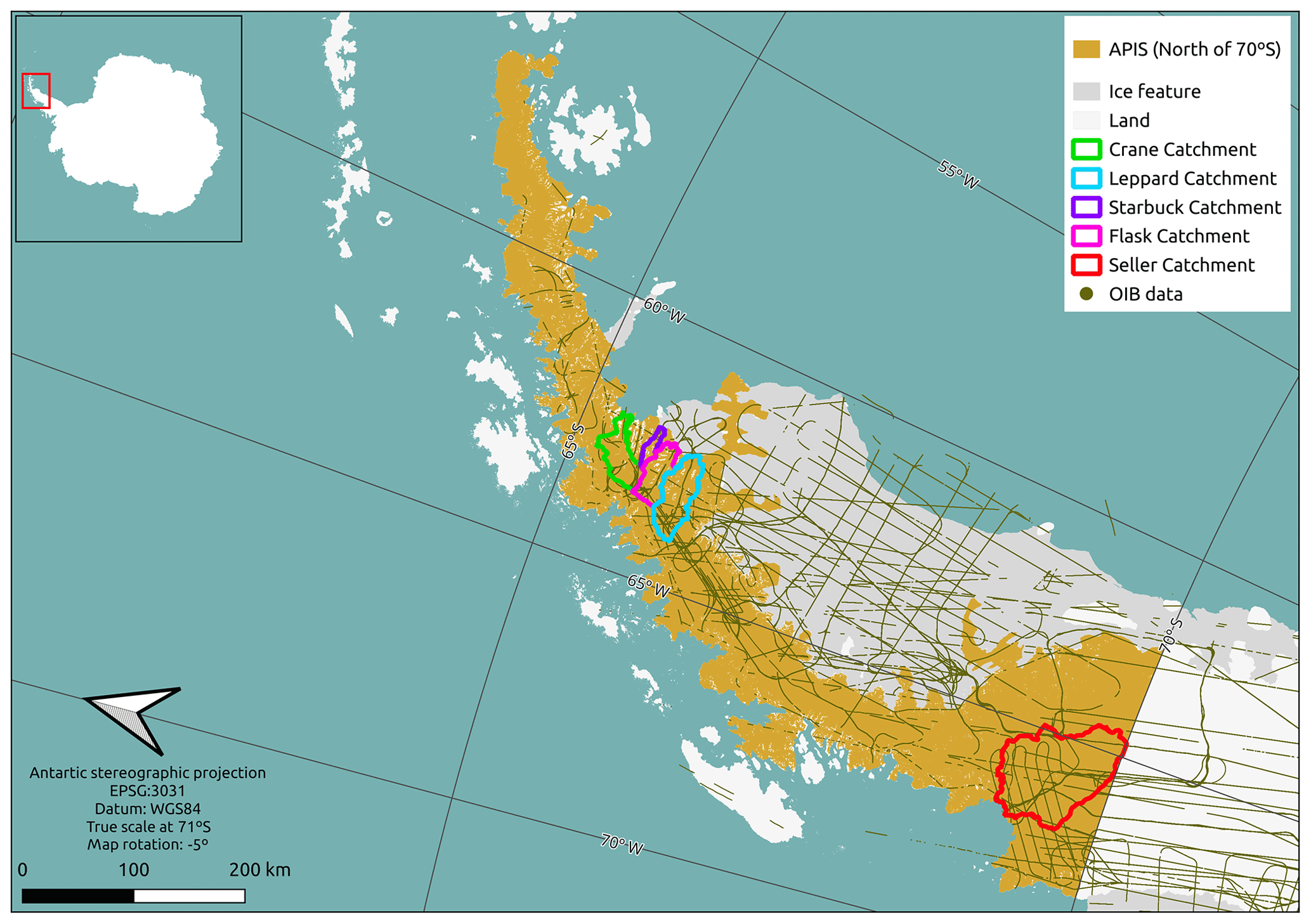
Figure 1 Study site with the five glacier catchments of interest and radar flight lines of Operation IceBridge (OIB).

2 Data

The data required by the two-step ice thickness reconstruction approach described in Sect. 3 include glacier outlines, a digital elevation model (DEM), surface elevation change, surface mass balance (SMB), ice thickness observations, and surface velocity fields. In the following, we describe these data in more detail.

2.1 Glacier outlines

The glacier outlines used in this study are adapted from Silva et al. (2020). They applied a supervised classification method to characterize glaciers in the AP region, specifically between the latitudes of 61 and 73° S, including the periphery. The classification was primarily based on the Advanced Spaceborne Thermal Emission and Reflection Radiometer (ASTER) imagery, ASTER Global Digital Elevation Map (GDEM), and Radarsat Antarctic Mapping Project (RAMP) DEM. To ensure continuity in the first step of the reconstruction process, the outlines were merged to treat the glaciers of the Antarctic Peninsula as a single entity. We also used data from the SCAR Antarctic Digital Database, such as rock outcrops (Gerrish et al., 2020), to better define the glacier outlines. The outline presented by Silva et al. (2020) also provided us with the free-boundary delineation of our inversion, as they used data from the SCAR Antarctic Digital Database to define the grounding line.

Several glaciers in the AP have a plateau-like upper part that flows towards the ocean through cliffs, which Gerrish et al. (2020) defined as rock outcrops due to the presence of exposed rock. Our reconstruction (see Sect. 3) would interpret these as zero ice thickness. Therefore, we manually removed such rock outcrops.

2.2 DEM

The digital elevation model (DEM) used in this study is the mosaic of the Reference Elevation Model of Antarctica (REMA) version 2 (Howat et al., 2022). REMA provides DEMs of the entire Antarctic continent at different resolutions. The elevation data in REMA are derived from satellite imagery, including WorldView-1, WorldView-2, WorldView-3, and GeoEye-1, using the SETSM software package (Howat et al., 2019), which employs stereography. For this study, the REMA mosaic with a 100 m resolution was chosen to match the resolutions of other relevant thickness maps, e.g., Carrivick et al. (2018) and Huss and Farinotti (2014), with acquisitions made between 2012 and 2020.

Due to the necessity of remedying the neglect of membrane stresses (Kamb and Echelmeyer, 1986), we applied the same smoothing technique as in Fürst et al. (2017), where the DEM is smoothed using ice thickness information. For the first iteration, we use H=100 m as a first guess. We invite the interested reader to view the work of Fürst et al. (2017) for a complete description of the smoothing technique.

2.3 Surface elevation change

The surface elevation change data used in this study were provided by Seehaus et al. (2023). They computed the average elevation changes in the Antarctic Peninsula region north of 70° S over the period of 2013–2017. The elevation change data were derived using differential interferometric synthetic aperture radar (SAR) from the TanDEM-X satellite mission. The SAR data were acquired during the austral winter to minimize the impact of differences in the penetration of the SAR signal into the snow/ice surface (Rott et al., 2018).

2.4 Surface mass balance

We obtained the SMB information for the 2008–2022 period from the regional climate model MARv3.12 (Modele Atmosphérique Régional), with a spatial resolution of 7.5 km, expressed in millimeters of water equivalent per year ($\mathrm{mm}\mathrm{w}.\mathrm{e}.{\mathrm{a}}^{-\mathrm{1}}$). It is a regional 3D atmosphere–snowpack model coupled with the SISVAT (Soil Ice Snow Vegetation Atmosphere Transfer) model intended to simulate surface processes. Further information on the evaluation and parameterization of the MAR model on the AP can be found in Dethinne et al. (2023).

We calculated the average value of the SMB during the 2011–2020 period to use as input to our model, with a resolution of 7.5 km, and downscaled it to a 100 m resolution using the REMA DEM, following a procedure similar to that of Huss and Farinotti (2014), who applied a linear relationship between SMB and elevation. We used a sample size of 11×11 pixels of the original SMB data (each pixel with a 7.5 km×7.5 km resolution) to compute a linear regression with respect to a resampled REMA DEM with the same resolution as the SMB (7.5 km). By applying the linear regression to the original DEM (100 m resolution), we obtained a downscaled SMB with a 100 m resolution. To obtain a smooth solution, we finally applied a moving average filter with a window size of 11×11 pixels to the downscaled SMB.

2.5 Ice thickness measurements

The ice thickness measurements used in this study were derived from data collected by Operation IceBridge (OIB; MacGregor et al., 2021) from NASA and by the Alfred Wegener Institute (AWI; Braun et al., 2018a, b, c, d). OIB collected data from multiple instruments during the period of 2009–2021. The AWI data specifically cover November 2014. The ice thickness measurements were obtained using airborne ground-penetrating radar. Due to the large number of points provided by OIB and AWI, data reduction became necessary. Upon testing, we decided to keep only thickness measurements with a minimum distance of 500 m. Additionally, measurements with clear inconsistencies, such as thick ice in ice-free areas or on mountain ridges, were manually removed from the data set.

2.6 Velocity field

We used velocity data processed and provided by ENVEO (Environmental Earth Observation IT GmbH) as part of the Antarctic Ice Sheet Climate Change Initiative project of the European Space Agency (https://cryoportal.enveo.at/data/). It consists of monthly Antarctic ice velocity mosaics derived from Sentinel-1 synthetic aperture radar (SAR) using feature-tracking techniques for the 2014–2021 period. The data are provided with a 200 m resolution in stereographic projection (EPSG:3031). The horizontal velocity components (in the x and y grid directions) are provided in true meters per day. From these data, we calculated a mean velocity field for the 2015–2017 period in the Antarctic Peninsula region north of 70° S. Figure D1 shows the magnitude of the velocity field.

3 Methods

We based our ice thickness reconstruction on Fürst et al. (2017) (other works such as Fürst et al., 2018; Sommer et al., 2023; and Fürst et al., 2024, have also used the same methodology), which consists of a two-step inversion method implemented in Elmer/Ice, an open-source finite-element software for modeling ice sheets, glaciers, and ice flow (Elmer/Ice, 2022). This approach applies the shallow-ice approximation and perfect plasticity in the first step, which gives a first estimate of the ice thickness. The aim of the first step using SIA is to calculate the ice flux (F) from the SMB (${\dot{b}}_{\mathrm{s}}$) and the local ice thickness change rate ($\partial H/\partial t$). In parallel to the SIA, we used the PP approach based on Linsbauer et al. (2012), which assumes that the local stress in the glacier is equal to the material-specific yield stress, which requires only the glacier geometry as input. For both models, we did the inversion using the latitude of 71° S as the southern boundary of our domain, where we set a free-boundary condition. Subsequently, we removed the results from 71 to 70° S, the latter becoming the southern limit of our results. Since both assumptions are sensitive to slope and are not suitable for flat regions such as those near the glacier termini (a threshold must be defined when the slope approaches zero), we then applied the second step, which updates the model in those areas with the available reliable velocity information (see the flow chart in Fig. 2). These regions (see the areas where the second step was applied in Fig. D1) overlap with the areas that are more prone to failure of the SIA and PP, therefore improving our reconstruction. Finally, both approaches were combined into a final thickness map by averaging the two results. All the thickness maps generated have the same 100 m resolution as the input DEM.

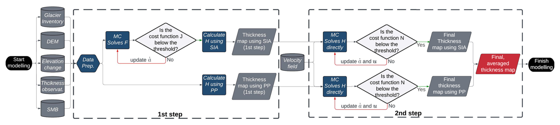
Figure 2 Flowchart depicting the ice thickness reconstruction process. The first step involves calculating the ice thickness (H) using either the shallow-ice approximation (SIA) or the perfect plasticity (PP) approach. In the SIA-based first step, the flux field (F) is determined by solving the mass conservation equation (MC) (Eq. 2). The flux field calculated is then evaluated by the cost function (J) (Eq. 3), which iteratively updates the apparent mass balance ($\dot{a}$) until the stopping criterion is met. At this stage, the flux map is utilized to calculate the ice thickness map (H) using the shallow-ice approximation (SIA) (Eq. 4). Alternatively, the PP approach uses the glacier outlines and elevation field to infer the ice thickness (Eq. 5). In areas with reliable velocity observations ($\left|u\right|\ge \mathrm{200}$ m a⁻¹), we perform the second step (see Fig. D1 for the areas with $\left|u\right|\ge \mathrm{200}$ m a⁻¹). Each previously generated thickness map from the first step is used as a boundary condition to directly calculate H by solving the mass conservation equation. The resulting ice thickness map is then improved using the cost function (N) (Eq. 6), which updates the values of $\dot{a}$ and u. The process continues until the stopping criterion is met (i.e., the cost function falls below a given threshold), resulting in the ice thickness maps using SIA and PP. Finally, the results of both approaches are combined by calculating the average value for each pixel, generating the final ice thickness distribution.

3.1 First step

3.1.1 Shallow-ice approximation

The method used in the present work to reconstruct the ice thickness (Fürst et al., 2017) is based on mass conservation. Assuming that ice is incompressible, mass conservation can be formulated as (Cuffey and Paterson, 2010)

$$\begin{array}{}\text{(1)}& {\displaystyle }{\displaystyle \frac{\partial H}{\partial t}}+\mathrm{\nabla }\cdot \left(\mathit{u}H\right)={\dot{b}}_{\mathrm{s}}+{\dot{b}}_{\mathrm{b}},\end{array}$$

where $\frac{\partial H}{\partial t}$ is the local temporal change in ice thickness, u is the horizontal depth-averaged velocity vector, H is the ice thickness, and ${\dot{b}}_{\mathrm{s}}$ and ${\dot{b}}_{\mathrm{b}}$ are the surface and basal mass balances, respectively. ∇⋅ is the 2D horizontal divergence. Rearranging Eq. (1), we can obtain

$$\begin{array}{}\text{(2)}& {\displaystyle }{\displaystyle }\mathbf{\nabla }\cdot \mathit{F}=\dot{a},\end{array}$$

where $\mathrm{\nabla }\cdot \mathit{F}=\mathrm{\nabla }\cdot \left(\mathit{u}H\right)$ is the 2D flux divergence, and $\dot{a}$ is the apparent mass balance ($\dot{a}={\dot{b}}_{\mathrm{s}}-\partial H/\partial t$), which combines all sources and sinks but neglects the basal mass balance (${\dot{b}}_{\mathrm{b}}$). To infer the flux direction, we assumed that the flux follows the steepest descent on the surface topography.

The ice flux solution in the first step often shows high spatial variability and negative values. Therefore, to reduce undesirable characteristics, we iteratively update the apparent mass balance ($\dot{a}$) as a control variable using a cost function J:

$$\begin{array}{}\text{(3)}& {\displaystyle }\begin{array}{rl}J& ={\mathit{\lambda }}_{\text{pos}}\cdot \underset{\mathrm{\Omega }}{\int }{F}^{\mathrm{2}}\underset{-\mathrm{\infty }}{\overset{-F}{\int }}\mathit{\delta }\left(s\right)\mathrm{d}s\mathrm{d}\mathrm{\Omega }\\ & +{\mathit{\lambda }}_{\text{reg}}\cdot \underset{\mathrm{\Omega }}{\int }\left[{\left({\displaystyle \frac{\partial F}{\partial x}}\right)}^{\mathrm{2}}+{\left({\displaystyle \frac{\partial F}{\partial y}}\right)}^{\mathrm{2}}\right]\mathrm{d}\mathrm{\Omega }\\ & +{\mathit{\lambda }}_{\dot{a}}\cdot \underset{\mathrm{\Omega }}{\int }{\left(\dot{a}-{\dot{a}}_{\text{init}}\right)}^{\mathrm{2}}\mathrm{d}\mathrm{\Omega },\end{array}\end{array}$$

where δ(s) is the Dirac delta function, with s∈ℝ. λ_pos,λ_reg, and ${\mathit{\lambda }}_{\dot{a}}$ are multiplier terms whose values were optimized in Fürst et al. (2017) to 10²,10⁰, and 10⁻², respectively, and Ω is the APIS domain. For the minimization of the cost function J, we rely on the module m1qn3 in Elmer/Ice (Gilbert and Lemaréchal, 1989), with a stopping criterion of 10⁻¹⁴, calculated as the ratio $|J_n-J_{n-\mathrm{1}}|/J_{n-\mathrm{1}}$, where J_n and J_n−1 are the values of the cost function for the current and previous iteration. The first term on the right-hand side of Eq. (3) penalizes solutions with negative flux since the integral over s of δ(s) with integration limits of −∞ and −F is zero if F is positive and 1 if F is negative. The integration over the APIS domain of F² multiplied by the integral mentioned above increases the penalization for regions with more negative flux values. The second term increases with higher variability in F; in this way, it favors smoother solutions. Finally, the third term penalizes the difference between the iteratively updated $\dot{a}$ and the initial apparent flux divergence input (${\dot{a}}_{\text{init}}$), limiting the deviation of $\dot{a}$ from the inputs of SMB and $\partial H/\partial t$. Ultimately, the cost function J is only a function of $\dot{a}$ since F is also a function of $\dot{a}$ (Eq. 2).

After the stopping criterion is reached, the ice flux is translated into ice thickness (H) in a postprocess using the shallow-ice approximation. The SIA assumes that the geometry of the glacier has a large aspect ratio (horizontal compared with vertical scales) (Hutter, 1983):

$$\begin{array}{}\text{(4)}& {\displaystyle }{\displaystyle }{F}^{*}={\displaystyle \frac{\mathrm{2}}{n+\mathrm{2}}}{B}^{-n}(\mathit{\rho }g{)}^n\Vert \mathrm{\nabla }h{\Vert }^n\cdot H^{n+\mathrm{2}},\end{array}$$

where F^* is the corrected flux (see Appendix A); B is the viscosity parameter, which is a priori unknown but can be calculated at points where ice thickness measurements are available (e.g., flight measurements of Fig. 1) using the same equation; and the flux field is calculated from the mass conservation described above. The viscosity parameter (B) is then spatially interpolated. To minimize extrapolation artifacts, we implemented a new approach in which we prescribed a value of B equal to the mean value of B calculated over the points along the domain boundary with ice thickness measurements, previously removing the upper and lower 10 % quantiles. ρ and g are the ice density (917 kg m⁻³) and the acceleration of gravity (9.18 m s⁻²), respectively. Equation (4) assumes that there is only ice displacement due to deformation, neglecting basal sliding, which limits its application to slow-moving areas. We remove this constraint in the second step of the reconstruction, where we solve Eq. (2) using the velocity information directly (without the need of the SIA). To avoid having Eq. (4) diverging to infinity when solving for H, we set $\Vert \mathrm{\nabla }h\Vert =\tan \left(\mathrm{1}\mathit{°}\right)$ wherever the slope is less than 1°.

3.1.2 Perfect plasticity

Another approach, which uses only glacier geometry to infer the ice thickness (H), is the perfect plasticity approach:

$$\begin{array}{}\text{(5)}& {\displaystyle }{\displaystyle }H={\displaystyle \frac{{\mathit{\tau }}_{\mathrm{d}}}{\mathit{\rho }g\tan \mathit{\alpha }}},\end{array}$$

where again ρ and g are the ice density and acceleration of gravity, respectively; α is the surface slope; and τ_d is the driving stress, which is a function of the material-specific yield stress (τ₀). As in the case of SIA, we calculate τ_d at points with ice thickness measurements using Eq. (5), and we then interpolate τ_d over the entire glacier domain, prescribing the mean value of τ_d of the entire domain (excluding the upper and lower 10 % quantiles) at the domain boundaries, as was done in the SIA approach. With the map of τ_d and surface slope (from the DEM), we can infer the ice thickness. Similarly to what we have done in the SIA case, in areas with α<1°, we set α=1° to avoid having Eq. (5) diverging to infinity.

3.2 Second step

In areas with reliable velocities (Fig. D1 shows the areas where we applied the second step), we perform the second step, in which the equation of mass conservation (Eq. 1) is directly solved using all the inputs used in the first step, with the only additional information being the surface velocity observations. In this way, the only unknown variable in Eq. (1) is the ice thickness H. Due to the fact that the velocity field (u) in Eq. (1) is a 2D vertically averaged vector and the second step is applied only to fast-flowing regions ($\left|u\right|\ge \mathrm{200}$ m a⁻¹), we opted to set the vertically averaged velocity to be equal to the surface velocity. This assumption neglects internal deformation, which is not unrealistic since in these regions basal sliding is expected to dominate (Bueler and Brown, 2009). We also used this velocity threshold because remote-sensing-derived velocity fields usually contain gaps, and the uncertainty can dominate the signal in slow-moving areas.

In the second step, the domain of fast-flowing regions (a subdomain of the glacier outline) requires lateral boundary conditions, which come from the first step from either the SIA or the PP solution fields. We set the ice thickness calculated from the first step as a Dirichlet boundary condition along the lateral margins of the fast-flowing domain. On the marine ice front, we apply a free-boundary condition.

Once we get the ice thickness map from the second step by solving the mass conservation equation, we use a cost function similar to Eq. (3) since we cannot ensure that the input data are consistent in terms of mass balance and the velocity field. To allow a better transition between the boundary condition and the regions where we apply the second step, we use the cost function:

$$\begin{array}{}\text{(6)}& {\displaystyle }\begin{array}{rl}N& ={\mathit{\gamma }}_{\text{pos}}\cdot \underset{\mathrm{\Omega }}{\int }{H}^{\mathrm{2}}\underset{-\mathrm{\infty }}{\overset{-H}{\int }}\mathit{\delta }\left(s\right)\mathrm{d}s\mathrm{d}\mathrm{\Omega }\\ & +{\mathit{\gamma }}_{\text{reg}}\cdot \underset{\mathrm{\Omega }}{\int }\left[{\left({\displaystyle \frac{\partial H}{\partial x}}\right)}^{\mathrm{2}}+{\left({\displaystyle \frac{\partial H}{\partial y}}\right)}^{\mathrm{2}}\right]\mathrm{d}\mathrm{\Omega }\\ & +{\mathit{\gamma }}_{\dot{a}}\cdot \underset{\mathrm{\Omega }}{\int }(\dot{a}-{\dot{a}}^{\text{init}}{)}^{\mathrm{2}}\mathrm{d}\mathrm{\Omega }\\ & +{\mathit{\gamma }}_{\mathrm{U}}\cdot \sum _{i=\mathrm{1}}^{\mathrm{2}}\underset{\mathrm{\Omega }}{\int }(u_i-u_i^{\text{init}}{)}^{\mathrm{2}}\mathrm{d}\mathrm{\Omega }.\end{array}\end{array}$$

As in the previous cost function (Eq. 3), the first and second terms in Eq. (6) are penalized for negative and highly variable ice thickness values, respectively. The third and fourth terms are intended to maintain the apparent flux divergence ($\dot{a}$) and velocity (u_i) close to their initial input values. Again, ${\mathit{\gamma }}_{\text{pos}},{\mathit{\gamma }}_{\text{reg}},{\mathit{\gamma }}_{\dot{a}}$, and γ_U are the multipliers of their respective terms. We chose to use the same values as in Fürst et al. (2017): ${\mathrm{10}}^{\mathrm{2}},{\mathrm{10}}^{-\mathrm{2}},{\mathrm{10}}^{-\mathrm{4}}$, and 10⁻⁸, respectively. The cost function N iteratively updates the values of apparent flux divergence and the velocity field until the same stopping criterion scheme of Eq. (3) is met.

Once the second step is completed, the results are two ice thickness maps: one based on SIA and another on PP, but both of them have the fast-flowing regions updated using velocity information. To produce a single ice thickness map, we then calculate a final ice thickness map by computing the mean value of the individual pixels of the SIA and PP reconstructions. This averaging of two different models is supported by the intercomparison of Farinotti et al. (2017, 2021), where they showed the advantages of ensemble models. Finally, the uncertainty estimation of the various steps is presented in Appendix B.

In what follows, to facilitate the discussion, we refer to the results of the first step using the SIA approach as S1SIA and to the results of the first step using the PP approach as S1PP. We refer to the outcome of averaging the results of S1SIA and S1PP as S1COMB. We use S1SIA & S2MC to refer to the results of applying the second step (updating the results from the first step using mass conservation in regions with velocities greater than 200 m a⁻¹) to S1SIA. Likewise, for the results of applying the second step to S1PP, we use S1PP & S2MC. Finally, S2COMB denotes the outcome of averaging the results of S1SIA & S2MC and S1PP & S2MC.

4 Results

Our results in Table 1 indicate that the total volume of ice in the APIS north of 70° is 27.4±12.0 (S1SIA & S2MC) or 27.9±12.2 (S1PP & S2MC) ×10³ km³. Considering an area of 81 535 km², we obtain mean ice thicknesses of 336 and 342 m, respectively. Furthermore, using the same methods and flux gates of Shahateet et al. (2023) (see Appendix C) resulted in ice discharge values of 95.4±12.4 and 99.7±12.9 km³ a⁻¹, respectively.

Table 1 Total volume and ice discharge calculated using the two approaches (SIA and PP), using the combination of both, using the first step only, and using the two steps. See Appendices B and C for details about error estimation.

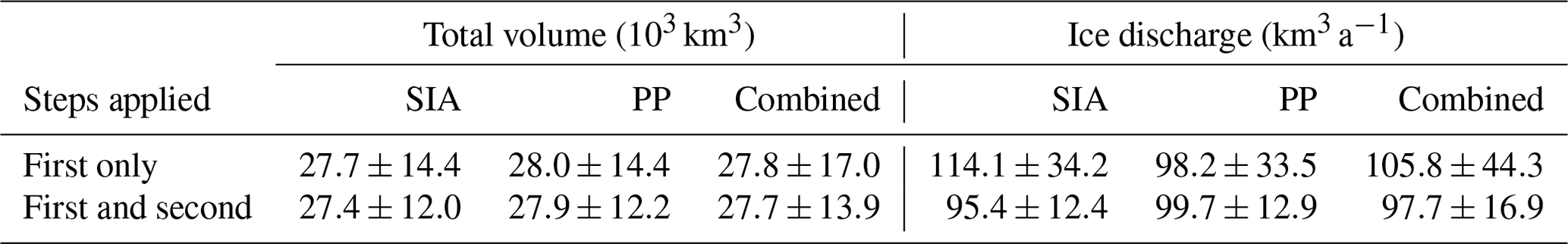
Table 1 also shows the impact of the second step on the ice discharge calculation. The ice discharge is more sensitive than the ice volume to the use of the second step since the latter is only applied to areas with large velocities, which include the zones upstream of the grounding lines and marine termini where the ice discharge is calculated. Regarding the changes implied by the introduction of the second step, the total volume decreased by 1.1 % from S1SIA to S1SIA & S2MC and by 0.4 % from S1PP to S1PP & S2MC. In the calculation of ice discharge, the introduction of the second step implied a decrease of 16.4 % from S1SIA to S1SIA & S2MC and an increase of 1.5 % from S1PP to S1PP & S2MC.

As the two assumptions (S1SIA & S2MC and S1PP & S2MC) led to similar results, we combined them in a final solution by calculating the mean value for each pixel. This resulted in a total volume of $\mathrm{27.7}\pm \mathrm{13.9}\times {\mathrm{10}}^{\mathrm{3}}{\mathrm{km}}^{\mathrm{3}}$ and an ice discharge of 97.7±16.9 km³ a⁻¹. The combined ice thickness distribution of S2COMB is shown in Fig. 3.

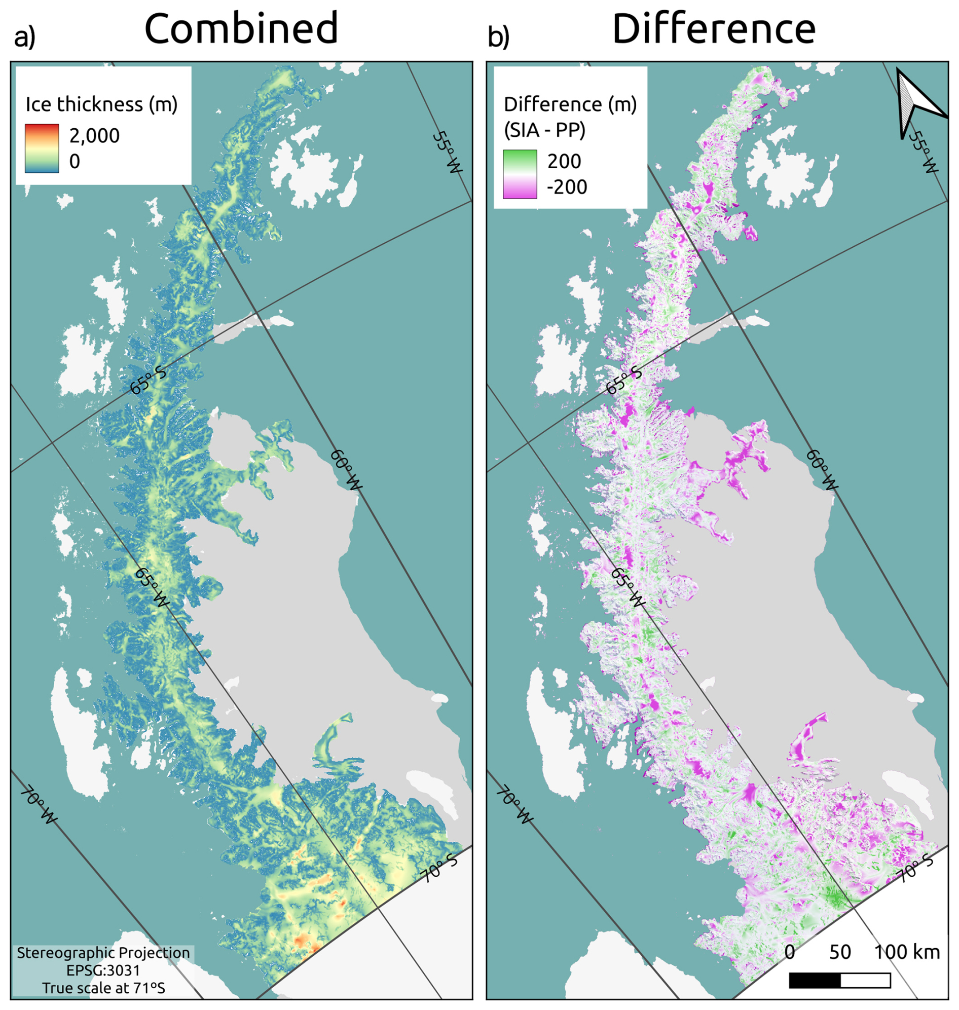
Figure 3 Ice thickness reconstructions using a two-step approach. (a) Combined is the average thickness of both approaches (S2COMB), and (b) difference is the difference between the results using the shallow-ice approximation (S1SIA & S2MC) and perfect plasticity (S1PP & S2MC) using the two steps. The colors on the difference scale are at 60 % transparency to enable the visualization of the optical image behind (© 2025 TomTom, Earthstar Geographics SIO).

5 Discussion

5.1 Discussion on the methodology

In general, the first step of the SIA and PP approaches produces ice thickness reconstructions consistent with the relief of our study site (ridges, valley glaciers, and ice caps on the AP plateau). We adjusted the glacier outlines by manually connecting the plateau ice to its outlet glaciers (see Sect. 2), as otherwise the ice thickness would be underestimated. The reason is that such unrealistic internal boundaries would imply zero-flux conditions and hence zero ice thickness.

The first step using the SIA (S1SIA) neglects basal sliding, which leads to an overestimation of the ice thickness in fast-flowing regions (see the differences in Fig. 3). In contrast, the introduction of the second step (resulting in S1SIA & S2MC) decreases the ice thickness values in fast-flowing regions when the SIA approach is used. Furthermore, SIA is sensitive to slope, specifically in flat areas near the terminus and on the plateau (see Eq. 4). The second step then improves the reconstruction in those regions, in particular near the marine termini. When the second step is applied to the PP approach (resulting in S1PP & S2MC), the ice discharge increases slightly. Although the PP approach is also sensitive to slope, it does not make any assumption about the velocity distribution throughout the glacier. Finally, Eq. (6) allows the reconstruction of ice thickness to pass smoothly from the first step to the second step. It updates the values of u and $\dot{a}$ to artificially produce a smooth change from no sliding (first step) to 100 % sliding (second step).

5.2 Comparison against previous regional-scale estimates

We now compare our results with the ice thickness maps most often used in the literature, namely Carrivick et al. (2018), Huss and Farinotti (2014), Fretwell et al. (2013), Leong and Horgan (2020), and Morlighem (2022). An important application of ice thickness reconstructions is the computation of ice discharge to the ocean. By combining the latter with the climatic mass balance, an estimate of the total mass balance is obtained (e.g., Rignot et al., 2019; Shepherd et al., 2018). Therefore, we focus on comparing the ice discharge estimates obtained when using the different ice thickness data sets. It is important to remark that as was done in Shahateet et al. (2023), the ice discharge computations are in all cases performed using the same set of flux gates and a common velocity field, so the differences in ice discharge between methods can be solely attributed to the differences in ice thickness at the flux gates. To analyze the differences in results between pairs of models, we used the equation introduced by Shahateet et al. (2023), where Δφ_jk represents a normalized mean difference in the calculation of ice discharge using models j and k for the whole set of flux gates:

$$\begin{array}{}\text{(7)}& {\displaystyle }{\displaystyle }\mathrm{\Delta }{\mathit{\phi }}_{jk}=\stackrel{\mathrm{‾}}{\left[{\displaystyle \frac{|{\mathit{\phi }}_{i,j}-{\mathit{\phi }}_{i,k}|}{\frac{\mathrm{1}}{\mathrm{6}}\left({\sum }_{l=\mathrm{1}}^{\mathrm{6}}{\mathit{\phi }}_{i,l}\right)}}\right]},\end{array}$$

where the fraction on the right-hand side represents the difference in the absolute value of the ice discharge calculated using the models j and k for the flux gate i, normalized by the mean of all models for that gate (the term in the denominator). The global average bar is understood to be applied over the whole set of flux gates (represented by the subscript i). The differences between our estimate of ice discharge and those of other authors are summarized in Table 2.

Table 2 Mean of the normalized difference in ice discharge between our model (S2COMB) and other models (see Eq. 7).

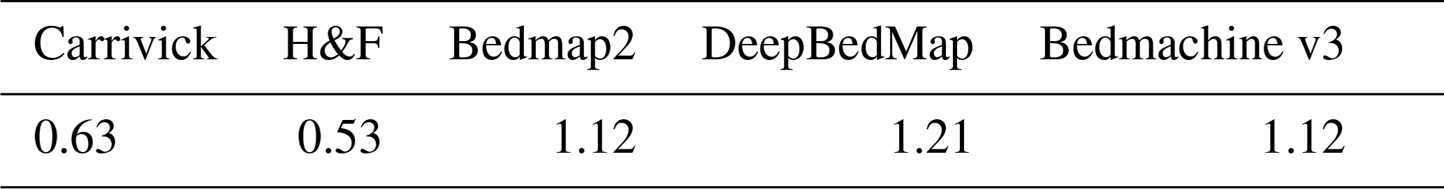
Table 2 shows that the results can be grouped into two different families. On the one hand, we have the physically based approaches (namely Huss and Farinotti, 2014, and Carrivick et al., 2018), which have lower differences compared to our S2COMB result in terms of ice discharge of the individual basins, and on the other hand, we have the neural-network- and interpolation-based approaches (namely Leong and Horgan, 2020; Fretwell et al., 2013; and Morlighem, 2022), with larger differences in comparison to our results. Note that although Morlighem (2022) used mass conservation to infer the ice thickness of the whole of Antarctica, in the APIS they mainly used anisotropic diffusion, so we put their APIS reconstruction into the interpolation-based group. When considering the total ice discharge estimate (Table 3), our model result is in between the two families, with the difference in total discharge between our model and that of Huss and Farinotti (2014) being similar to the difference between our model and Bedmap2 (and DeepBedMap), and the difference between our model and Carrivick's is similar to the difference between our model and Bedmachine.

We also observe in Table 3 that our model produces a total ice volume very close to that of Huss and Farinotti (2014), which is also the result showing the closest ice discharge to our own estimate. Comparing the ice discharge of our first step reconstruction using S1SIA (Table 1), which is an approach similar to that used by Huss and Farinotti (2014) based on mass conservation, results in 11 % lower discharge. The introduction of the second step in S2COMB produced an ice discharge value 24 % lower than that of Huss and Farinotti (2014). Regarding the total ice volume, S1COMB resulted in a value 5.5 % lower than that of Huss and Farinotti (2014), and it did not change significantly in S2COMB.

Table 3 Total ice volume and ice discharge calculated in the present work that make use of the two-step approach considering the shallow-ice approximation (SIA) and perfect plasticity (PP), which are combined into a final, single ice thickness field (S2COMB), and the results obtained using the different ice thickness models available in the literature for the Antarctic Peninsula north of 70° S (Carrivick et al., 2018 (Carrivick); Huss and Farinotti, 2014 (H&F); Fretwell et al., 2013 (Bedmap2); Leong and Horgan, 2020 (D.BedMap); and Morlighem, 2022 (B.machine v.3)). Carrivick et al. (2018) and Leong and Horgan (2020) do not provide error estimates of their ice thickness reconstructions.

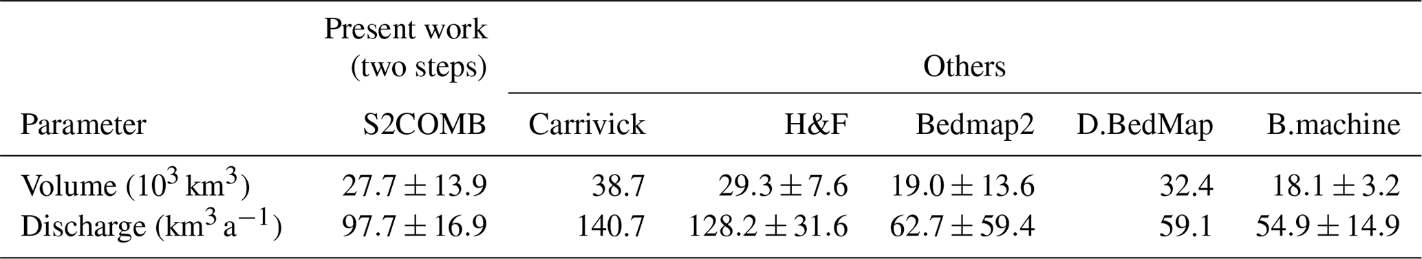
The differences are larger with respect to the reconstruction of Carrivick et al. (2018). S1PP (an approach similar to Carrivick et al., 2018) resulted in an ice discharge and total volume 30 % and 28 % lower, respectively, than those of Carrivick et al. (2018). When the second step was introduced and the two reconstructions were combined in S2COMB, the differences from Carrivick et al. (2018) remained almost equal to those of the S1PP, with ice discharge and total ice volume 32 % and 26 % lower, respectively. Although the results by Carrivick et al. (2018) are based on PP, their calculation of the driving stress (τ_d) is different. While we calculate τ_d by inversion of Eq. (5) and then interpolation throughout the domain, Carrivick et al. (2018) used an empirical relation proposed by Driedger and Kennard (1986) based on curve fitting between area, slope, and basal shear stress using data of the major glaciers of four Cascade Range volcanoes in North America, with areas ranging from 1.2 to 11.0 km², which have markedly different geometries compared to the AP glaciers. They then validated their fit using glaciers from other regions (which did not include glaciers in the AP) ranging from 1.0 to 4.1 km². The characteristics of the glacier used by them contrast with glaciers in the APIS north of 70° S. In this region, the glaciers range from 2.9 to 7000 km², with a mean area of 100 km². Therefore, the empirical relation proposed by Driedger and Kennard (1986) extrapolates most of the basal shear stress in our region of interest (63 % of the glaciers in the region are greater than 11 km²). Another characteristic of the empirical relationship that can lead to an overestimation of the basal shear stress in the APIS is the fact that the elevation range in volcano glaciers is usually greater than the elevation range of the APIS glaciers, resulting in relatively fewer elevation bands (see Carrivick et al., 2018), which implies even larger areas of the individual elevation bands. Furthermore, implicit in their assumption is the fact that larger glacier areas correspond to thicker ice (which would result in greater basal shear stress). But in the case of the APIS glaciers, this could be achieved through a different relationship from that of Driedger and Kennard (1986), given the completely different geometry of both sets of glaciers.

Regarding the comparison with the neural-network- and interpolation-based models of Tables 2 and 3 (Leong and Horgan, 2020; Fretwell et al., 2013; Morlighem, 2022), our results are substantially larger for both ice volume and ice discharge, except for the ice volume calculated by Leong and Horgan (2020), which is similar to our own estimate. The largest difference in the calculation of the ice discharge (Δφ) with respect to our model is that of the Bedmachine model.

Shahateet et al. (2023) noted that the Bedmachine v2 model (Morlighem et al., 2020) used mainly anisotropic diffusion to estimate the ice thickness in the Antarctic Peninsula, except for three glaciers, namely the Flask, Leppard, and Seller glaciers. This anisotropic diffusion is a type of interpolation in which the quality of the reconstruction can be highly impacted by the lack or scarcity of ice thickness measurements (which is also the case for Bedmap2 since it is a pure interpolation method). Shahateet et al. (2023) highlighted that Bedmachine v2 shows 24 % near-zero ice thickness values (a situation close to that of Bedmap2) along the flux gates that they used to calculate the ice discharge of the APIS. This explains their low ice discharge values. In fact, when we compare our ice discharge estimates from S2COMB with those of Bedmachine v3, restricting comparison to the three glaciers where they applied mass conservation, the differences decrease substantially. The normalized differences in the ice discharge calculation between these two models (see Eq. 7) for the Flask, Leppard, and Seller glaciers are 0.45, 0.29, and 0.22, respectively. These differences in the ice discharge calculation contrast markedly with the value of 1.12 obtained when all of the APIS glaciers are considered (Table 2). This shows that when Bedmachine v3 applies mass conservation (in fast-flowing glaciers), they produce ice discharge estimates closer to our own ones.

Focusing now on the differences from DeepBedMap, we note that they used a super-resolution deep-convolutional neural network trained with Antarctic data external to the AP, which may have affected the final solution in our region of interest. Furthermore, Shahateet et al. (2023) demonstrated the high variability and the large number of negative ice thickness values in the DeepBedMap reconstruction of the APIS (we masked such negative ice thickness values to zero thickness values in our calculations using their model). Finally, Figs. 4 and D3 show that the three reconstructions mentioned (Bedmap2, DeepBedMap, and Bedmachine) may underestimate the ice thickness in the valley glaciers of the AP.

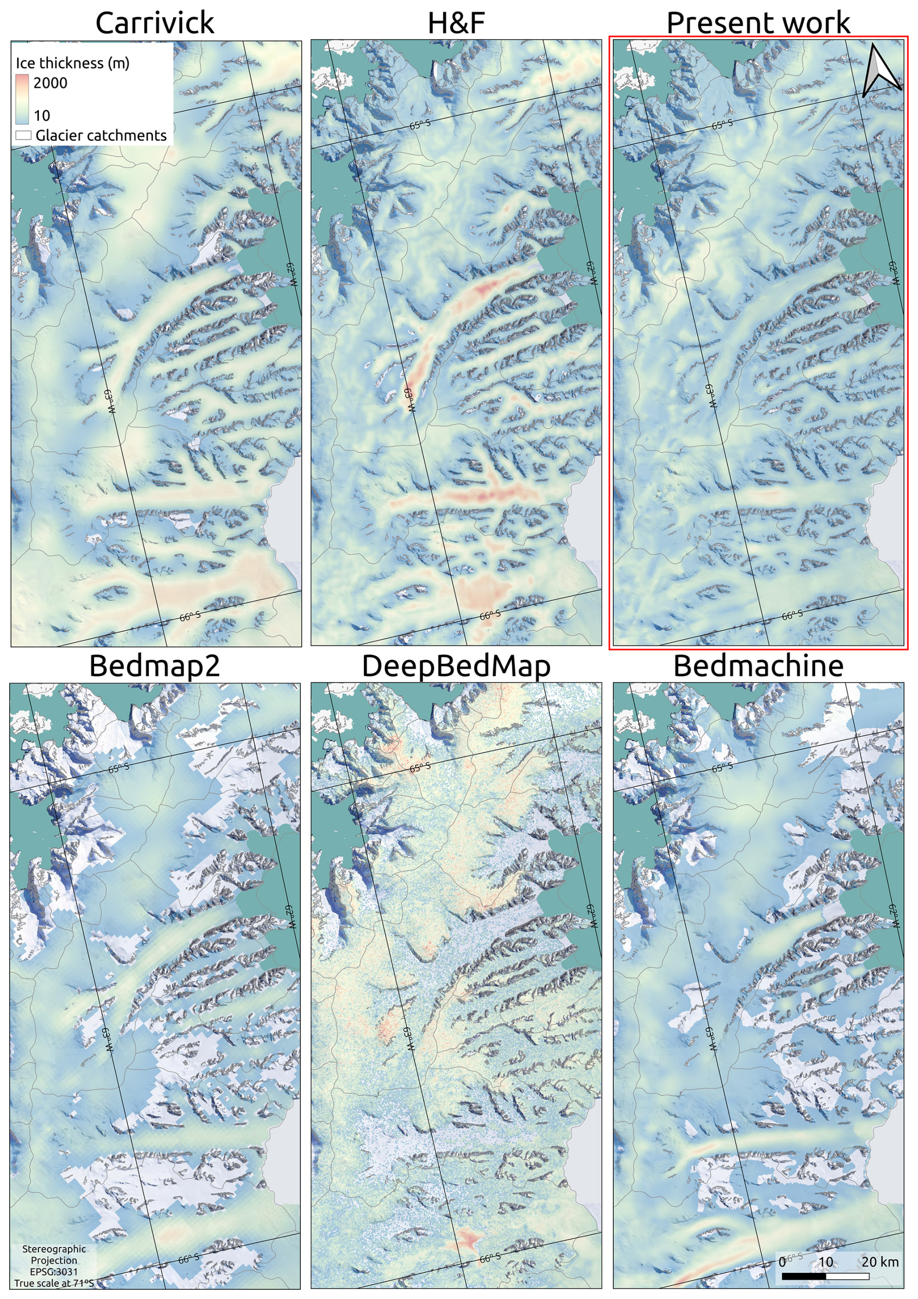
Figure 4 Close-up of the reconstructions of Carrivick, H&F, the present work, Bedmap2, DeepBedMap, and Bedmachine v3 on the region surrounding the Crane, Starbuck, Flask, and Leppard glaciers, all of which flow towards the embayment of the former Larsen B Ice Shelf. The colors on the ice thickness scale are at 60 % transparency to enable the visualization of the optical image behind (© 2025 TomTom, Earthstar Geographics SIO). We masked ice thickness values lower than 10 m.

Regarding the spatial distribution of the differences in ice discharge calculated using the different models, Fig. D4 shows the multimodel normalized root-mean-square deviation (Shahateet et al., 2023) among the different models. As in Shahateet et al. (2023), it illustrates the inhomogeneous spatial distribution of the differences. In particular, the higher similarity in results for the glaciers terminating in ice shelves compared to those terminating in the ocean is remarkable. Shahateet et al. (2023) attributed this unequal spatial distribution to the fact that there are more abundant radar flight lines on glaciers that end on ice shelves, thus better constraining the models. This highlights the importance of undertaking further ice thickness measurements to reduce the uncertainty in the calculated ice discharge and total volume.

5.3 Comparison with radio-echo sounding data

Since our final ice thickness map is S2COMB, the discussion presented hereafter will refer to it as the result of the present work.

To validate the performance of the different models at the single-glacier scale, we used radio-echo sounding (RES) data from Farinotti et al. (2013) on the Flask and Leppard glaciers, which were acquired in 2010 and 2011. Farinotti et al. (2013) used an ice flow model to reinterpret the RES data, categorizing the ice thickness measurements into a clear, easy-to-interpret signal and a very diffuse, speculative signal. Farinotti et al. (2013) also identified signals that are probably reflections from the bed and signals that are probably reflections from the side walls. With the aim of comparing the different models available for the APIS north of 70° S, we calculated the normalized mean absolute error (NMAE; see Shahateet et al., 2023) of the individual models with respect to the RES measurements of Farinotti et al. (2013), using only their better-quality P01, P02, and P03 ice thickness measurements (see Fig. 5a).

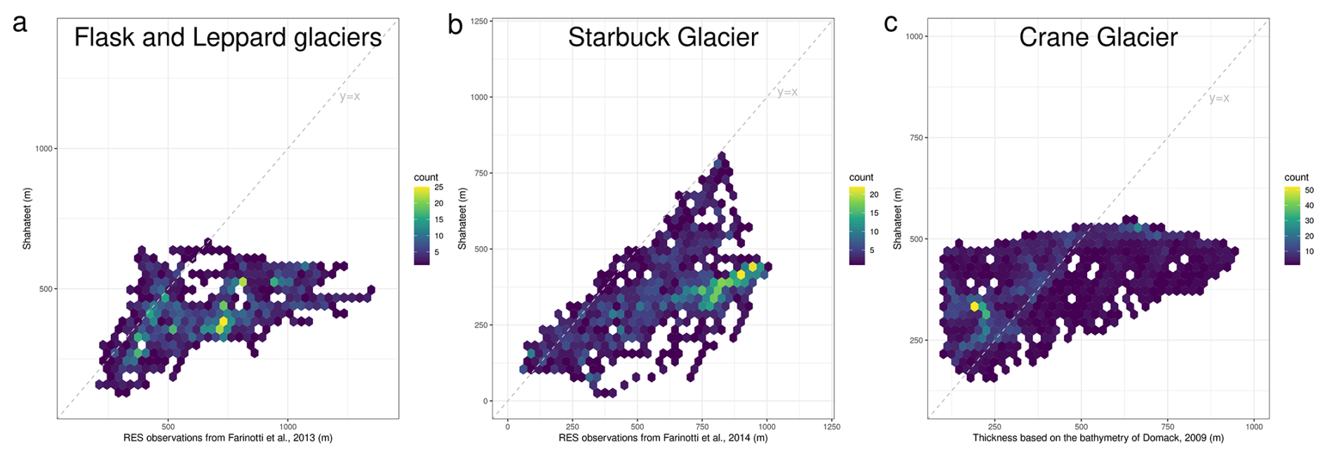
Figure 5 Hexagonal binned plots of three different sources compared to our reconstruction: (a) radio-echo sounding (RES) of the Flask and Leppard glaciers from Farinotti et al. (2013), (b) RES of the Starbuck Glacier from Farinotti et al. (2014), and (c) inference of ice thickness using DEM from REMA. The bathymetry is from Domack (2009).

The lowest NMAE of all six reconstructions corresponds to Bedmap2, at 29 %. Our reconstruction and that of Bedmachine v3 had similar NMAEs of 35 % and 33 %, respectively. DeepBedMap, Carrivick, and H&F had similar values: 58 %, 60 %, and 66 %, respectively. Due to easy access to the input data used by Bedmap2 (see Fretwell et al., 2013), we can analyze the reason why Bedmap2 has a lower error than our reconstruction on the Flask Glacier. Both inversions used the OIB data from 2011, but Fretwell et al. (2013) managed to identify data from ice thickness measurements with high uncertainty, excluding them from their reconstruction. Therefore, when they used their method to interpolate the ice thickness, they had good data overlapping the same region where Farinotti et al. (2013) had high-quality data.

Although the reanalysis by Farinotti et al. (2013) constitutes the most reliable validation data for the ice thickness in the AP available in the literature, their analysis covers only the Flask and Leppard glaciers, forcing us to use other resources to validate the models. These include RES measurements on the Starbuck Glacier from 2012 (Farinotti et al., 2014) (Fig. 1). These data were used as input to the ice thickness inversion of Huss and Farinotti (2014), so they cannot be used to validate their bed reconstruction. The velocity field on the Starbuck Glacier used in the present work is below 200 m a⁻¹; consequently, for this specific glacier, we only performed the first step of our two-step approach.

Figure 5b shows the hexagonal binned (hexbin) chart of the thicknesses of Farinotti et al. (2014) and of the present reconstruction. Compared to the other reconstructions, Carrivick's solution and our own had similar NMAEs with respect to the RES measurements, at 37 % and 42 %, respectively. Bedmap2, DeepBedMap, and Bedmachine v3 had values of 73 %, 63 %, and 91 %, respectively. The NMAE of H&F with respect to the RES measurements, 27 %, cannot be considered for validation because, as mentioned earlier, these data were used for calibration of their ice thickness reconstruction. But this analysis helps to highlight the close performance of Carrivick's reconstruction and our own in comparison to H&F, which used the measurements in their reconstruction.

The independent data on the Flask and Starbuck glaciers used to validate the models highlights the marked errors in all reconstructions but shows that the present work is among the reconstructions presenting lower errors for the two glaciers analyzed.

Due to the lack of other reliable field measurements, we used indirect measurements of ice thickness to evaluate the reconstructions. In the following, we use bathymetric data together with elevation to estimate the ice thickness of the Crane Glacier. According to Needell and Holschuh (2023), the Crane Glacier (see location in Fig. 1) experienced a retreat of more than 10 km after the collapse of the Larsen B Ice Shelf during 2002–2004. After that, the glacier front was relatively stable until 2010, when the glacier started to readvance until 2021. In 2006 (during the stable period when the glacier had retreated), Domack (2009) acquired bathymetric data from the Crane Glacier embayment. With the readvance of the Crane Glacier, this bathymetry became bed topography near the glacier terminus. Using these data together with the surface elevation from REMA, we inferred the thickness primarily using the sum of the bathymetry and the elevation. Basically, if the surface elevation (h) was $\ge \frac{\mathrm{1}}{\mathrm{9}}$ of the seafloor depth (d), we then set $H=h+d$. However, there were some regions where the surface elevation was $<\frac{\mathrm{1}}{\mathrm{9}}$ of the seafloor depth within the region defined as grounded ice by our input data. Therefore, in these raster cells, we assumed that the ice was floating (thus H=10 h, where H is the thickness, and h is the surface elevation). Although we did not aim to infer ice thickness in floating ice, since this area of the Crane Glacier is a fast-flowing region where we applied the second step, we expect the model to be a good approximation of the ice thickness near the grounding line of this region.

Figure 5c shows the hexbin chart of this reconstruction of ice thickness in the front of the Crane Glacier and our two-step reconstruction. Again, we used the NMAE to evaluate the performance of the reconstructions. The lowest NMAE was found for Bedmap2, with an NMAE of 46 %, followed by our reconstruction at 66 %. Carrivick, H&F, and Bedmachine v3 had NMAEs of 72 %, 79 %, and 99 %. The NMAE of Bedmachine v3 was close to 100 % due to the large number of zero ice thickness values. Finally, DeepBedMap resulted in an NMAE of 183 % without removal of the negative values of ice thickness and 94 % when the negative values were set to zero (see Shahateet et al., 2023, for a complete discussion of the negative ice thickness values of the DeepBedMap reconstruction). Part of the large NMAE can be attributed to the error in the DEM data since every meter of uncertainty in the DEM will be multiplied by 10 when we apply the flotation criterion. Another important contributor to the uncertainty in the ice thickness reconstructions of this specific glacier is the fact that ice thickness measurements of the OIB were acquired in 2002, 2004, and 2016. Therefore, reconstructions made before 2016 only used OIB data from 2002 and 2004, which according to Needell and Holschuh (2023) was the period of retreat of the Crane Glacier. This contrasts with the data acquisition period used to mosaic the DEM of REMA (2012–2020) when the glacier was advancing. The REMA DEM was used to calculate the ice thickness of the Crane Glacier together with the flotation criterion assumption, which would reflect the ice thickness of its acquisition period. Even in the reconstruction proposed here, our algorithm (Sect. 2) selected the OIB data from 2002, which are precisely the same data used by Fretwell et al. (2013), and these are the two models with the lowest NMAEs in comparison to the ice thickness calculated in the Crane Glacier. We therefore attribute the large error to the high uncertainty in the input data of the models.

The reanalysis of Farinotti et al. (2013) mentioned previously also allows us to evaluate the quality of the ice thickness measurements used in our inversion, which in the Flask region consists of only OIB data. Figure 6 highlights the differences in the Flask Glacier between the OIB measurements and the reanalysis of Farinotti et al. (2013). Some points just 10 m apart in OIB and in Farinotti et al. (2013) data differ in ice thickness by more than 100 % (e.g., within 10.5 m, OIB measured a value of 1562 m, while the reanalysis of Farinotti et al., 2013, provided a value of 738 m). Even the OIB measurements sometimes lack self-consistency. In a specific case, for example, OIB provided ice thickness values of 1637 and 761 m for measurements points just 6 m apart. Other inconsistencies appear in the OIB data. For instance, there are measurements of thick ice (more than 500 m) over rock outcrops. Another zone (on the side mountains of the Hariot Glacier) with a steep slope had measurements of 2200 m in thickness. These inconsistencies can be due to incorrect flight line positioning data or the presence of temperate ice, which scatters the radar signal, making the identification of the bed more difficult. These problems result in unrealistic ice viscosity and driving stress in Eqs. (4) and (5), respectively, which especially affect our first-step estimates.

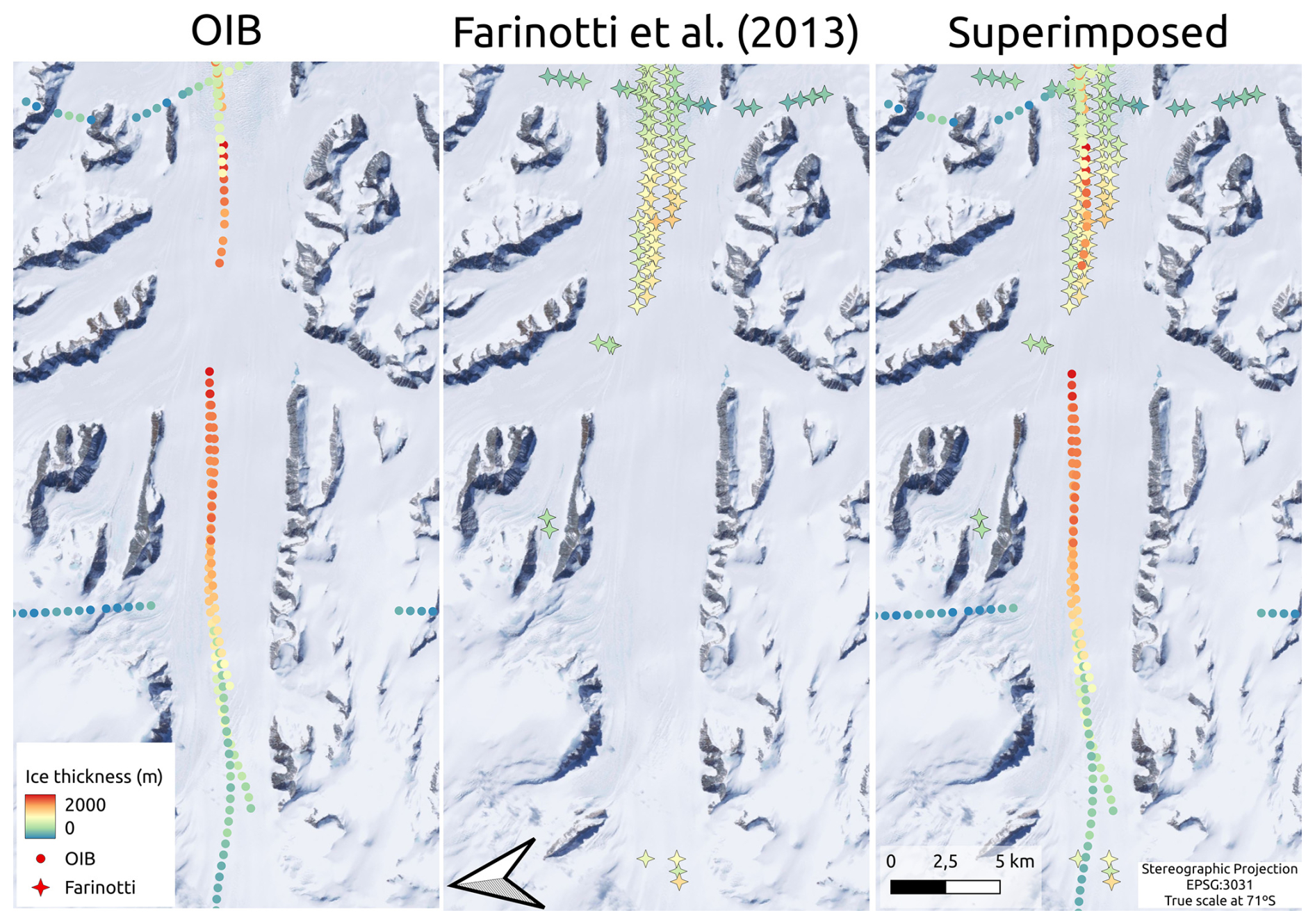
Figure 6 Ice thickness measurements on the Flask Glacier (see Fig. 1 for location). The first panel shows data from Operation IceBridge (OIB), while the second panel shows the reanalysis of Farinotti et al. (2013). Lastly, the third panel superimposes the two previous panels. The number of measurement points along the lines was reduced to allow for better visualization. Optical image © 2025 TomTom, Earthstar Geographics SIO.

5.4 Qualitative indicators of performance

Qualitatively, it is also possible to evaluate how well a given ice thickness reconstruction reproduces the features seen in a certain region. For example, the APIS region has some characteristic features, such as a plateau on the spine of the peninsula that accumulates ice, which then flows towards the ocean, often through very steep slopes and cliffs, frequently forming ice falls, and then the slopes become gentler in the outlet valley glaciers. We selected two regions with markedly different amounts of field data for qualitative analysis. The region in Fig. 4 was selected due to the large number of ice thickness measurements available (as seen in the previous analyses of the Crane, Starbuck, Flask, and Leppard glaciers), which provide more constraints on the reconstructions. In contrast, we selected the region in Fig. D3 (northern tip of the AP) due to the lack of measurements, which resulted in poor constraints on the reconstructions.

In Fig. 4, despite the thickness differences, we can see that the three reconstructions (Carrivick, H&F, and ours) reproduce thicker ice over the plateau, thinning toward the cliffs (due to increasing slope, thus accelerating the ice) and then thickening again in the valleys, with a flatter slope. The other three reconstructions (Bedmap2, DeepBedMap, and Bedmachine v3) shown in Fig. 4 also reproduce thicker ice on the plateau and a thinning near the cliffs but do not represent some glaciers in the valley regions well. In the case of DeepBedMap, a highly pixelated reconstruction is also shown.

In Fig. D3, we see again that Carrivick, H&F, and our model reconstruct thick ice on the plateau and a thinning when ice passes through the cliffs, thickening when the valleys are reached. Bedmap2 and DeepBedMap also reproduced the thicker ice on the plateau thinning toward the cliffs, again failing to reproduce the glaciers in the valleys. However, Bedmachine v3 did not properly reproduce the ice thickness in the northernmost part of this region, where it estimates ice thicknesses lower than 10 m.

5.5 Limitations

As shown by Farinotti et al. (2021) in an intercomparison experiment, the assumptions made by the different models have advantages and disadvantages for different regions and types of glaciers. Since complex ice–dynamics approaches are out of the scope of this paper due to the computational cost for large areas, in the APIS, all attempts to infer ice thickness make use of a simplifying assumption such as SIA or PP (apart from the models already mentioned, other studies that infer the ice thickness on a large scale are Millan et al., 2022, and Farinotti et al., 2019, which also use simplifying assumptions). These assumptions bring limitations, which we describe below.

First, the aim of these approaches is to use surface information to infer ice thickness. This leads to a limited horizontal representation of basal features that are smaller than the ice thickness in the corresponding area, since they do not leave surface expressions (Gudmundsson, 2003). As the basal slip increases, this limitation becomes even greater (Gudmundsson, 2003).

Second, in the specific case of the shallow-ice approximation, an assumption of the basal slip is required. Since the sliding of a glacier is notoriously difficult to measure, we needed to assume a value for this parameter, which we defined as zero for velocities up to 200 m a⁻¹. We based our assumption on the sensitivity analysis made by Huss and Farinotti (2014), where they varied the sliding parameter (giving as a ratio between the surface and the basal velocity) by ±20 %, resulting in variations of ±1.2 % in the final ice thickness. Summed up to the inversion of basal friction made by Morlighem et al. (2013), high values of basal friction appear in the higher elevations of the APIS, decreasing toward the terminus (where we apply the second step). Having said that, although the assumption of no sliding up to velocities of 200 m a⁻¹ is a strong assumption, the impact on our final result is limited.

Another limitation of our method relies on the fact that the use of SIA or PP requires the assumption of viscosity (B) and driving stress (τ_d), respectively. For these, we used the methodology of Fürst et al. (2017) (which proved to be useful in other regions) by interpolating (see Fig. D5) in situ measurements, as explained in Sects. 3.1.1 and 3.1.2. This approach favors the reproduction of individual point measurements of ice thickness rather than obtaining a spatially constant viscosity field. Interpolating B and τ_b has the disadvantage of assuming that adjacent grid points have similar characteristics, which can be unrealistic. We refrained from pursuing specific drainage basin values because these would introduce abrupt lines in the ice thickness field along the internal boundaries, especially in flat areas where the aspect ratios are large.

We tried to minimize the impact of these disadvantages by removing unrealistic measurements based on the analysis of all thickness surveys and by the removal of observations based on criteria such as poor geolocation or unreliable spatial variability. Moreover, the model applies an upper and lower viscosity threshold to remove further outliers. Lastly, the APIS geometry is characterized by many small ice-free patches within the glacierized area. Along these internal boundaries, the viscosity values are restored to the mean APIS values, avoiding extrapolation effects. However, these cannot ensure that all glacier catchments have a representative viscosity or driving stress, which is an inherent limitation of our method.

Finally, as shown in Sect. 5.3, our results still show a large error compared to the few independent measurements made in the region. This is an important aspect to take into account when using our reconstruction for single ice catchments. This is a limitation of all the reconstructions made in the APIS; our reconstruction, however, had in nearly all cases a comparatively lower error.

6 Conclusion and outlook

In the present work, we provide a new ice thickness map of the Antarctic Peninsula Ice Sheet north of 70° S. This map was constructed based on the two-step approach proposed by Fürst et al. (2017). The first step estimates the ice thickness distribution using two different approaches, namely the shallow-ice and the perfect plasticity approximations. For fast-flowing areas, the second step updates the ice thickness from the first step using mass conservation, with the aim of overcoming the limitations of SIA and PP near the glacier termini, where such approaches do not perform properly due to the low slopes. Finally, the results from both approaches are combined into a single ice thickness product. Using this product, we estimated a total volume of $\mathrm{27.7}\pm \mathrm{13.9}\times {\mathrm{10}}^{\mathrm{3}}$ km³ for the APIS north of 70° S and a total ice discharge of 97.7±16.9 km³ a⁻¹ over the period of 2015–2017, values that lie in the middle of the range the estimates by other authors, which show a large spread.

Comparing our results with those summarized in Shahateet et al. (2023) for the same region showed that our ice thickness reconstruction produces results similar to those of Huss and Farinotti (2014) in terms of spatial distribution of ice thickness, total volume, and ice discharge (especially when only SIA is applied) and comparable results to those of Carrivick et al. (2018) in terms of spatial distribution of ice thickness. On the other hand, our solution showed substantial differences from those of Fretwell et al. (2013), Leong and Horgan (2020), and Morlighem (2022). We attribute these similarities and differences of our model and those of Huss and Farinotti (2014) and Carrivick et al. (2018) to the use of physically based approaches, while Fretwell et al. (2013) and Morlighem (2022) used interpolation-based approaches, and Leong and Horgan (2020) used a super-resolution, neural-network-based approach based on Fretwell et al. (2013). All of these are highly affected by the scarcity of ice thickness measurements. Furthermore, we showed that the H&F and Carrivick reconstructions as well as ours qualitatively reproduced the features expected in the region, including thick ice on the plateau areas of the APIS, thinner ice on the high-slope areas in the transition zones from the plateau areas to the outlet glaciers draining them, and then thicker ice on the outlet valley glaciers. Bedmap2, DeepBedMap, and Bedmachine v3, however, failed to adequately reproduce some of these features.

All models showed large errors (NMAEs) when validated against independent ice thickness data. In the case of the most reliable set of independent data, namely that of Farinotti et al. (2013) on the Flask Glacier, errors ranged from 29 % to 66 %. This highlights the need for more dense and accurate field measurements of ice thickness in the APIS region, as proposed by the RINGS action group of SCAR. This is needed to reduce the uncertainties in total ice discharge and total volume, which have an impact on the projections of future contributions to sea level rise from ice wastage from this region.

Regarding the currently available ice thickness datasets, remarkable inconsistencies among them are sometimes present. Some of these inconsistencies could derive from improper positioning data of the radar flight lines and some from the presence of temperate ice, the latter especially in the northernmost regions. The usefulness of the available ice thickness data could be improved by reanalyses such as the one performed by Farinotti et al. (2013), involving a detailed quality check of the radio-echo-sounding data, leading to a classification of the measurements into a range from a clear, easy-to-interpret signal to a very diffuse, speculative signal. Also, reprocessing some problematic OIB flight lines could be beneficial to reduce uncertainties.

As the first step preserves the ice thickness observations, measurement errors were directly translated into our ice thickness maps. The second step was able to update the ice thickness in areas with velocities greater than 200 m a⁻¹. However, in slow-moving areas, the ice thickness was not updated, preserving the measurement errors. In the future, this could be refined by applying a cost function to the viscosity and driving stress fields, taking into account their absolute value and their variability, as well as including the temperature dependency of the viscosity.

Appendix A: Flux-based solution

Instead of applying the flux field (F) from Eq. (2) to directly invert the thickness field using Eq. (4), where the zero transitions in the flux field would be transmitted to the ice thickness solution, we corrected the flux field according to Fürst et al. (2017):

$$\begin{array}{ll}{\displaystyle }& {\displaystyle }{F}^{*}=(\mathrm{1}-\mathit{\kappa })\cdot \Vert F\Vert +\mathit{\kappa }\cdot F_{\text{crit}},\text{ where }\\ \text{(A1)}& {\displaystyle }& {\displaystyle }\mathit{\kappa }=\mathrm{1}-\mathrm{2}/\mathit{\pi }\cdot \text{arctan}(F^{\mathrm{2}}/F_{\text{crit}}^{\mathrm{2}}),\end{array}$$

where F_crit is defined as 10 % of the mean flux magnitude across the entire domain.

Appendix B: Error estimation of the ice thickness reconstruction

We first calculate the error in the first step using the shallow-ice approximation (and assume the same error for the perfect plasticity case) and then update the error values in areas where we performed the second step.

B1 Estimation of error in the first step

We calculate the error map in the first step (valid for both SIA and PP) using the SIA equations. The error in the ice thickness distribution stems from the uncertainty in the input fields of SMB and $\partial H/\partial t$. As in Fürst et al. (2017), we assume that the errors are transmitted through the mass conservation equation (Eq. 1) and are then scaled by the SIA when deriving the ice thickness from the flux (Eq. 4). We also assume that the inaccurate flux field (F+δF) also satisfies the mass conservation equation (Morlighem et al., 2014):

$$\begin{array}{}\text{(B1)}& {\displaystyle }{\displaystyle }\mathrm{\nabla }\cdot \left[\right(F+\mathit{\delta }F\left)\right(\mathit{n}+\mathit{\delta }\mathit{n}\left)\right]=\dot{a}+\mathit{\delta }\dot{a},\end{array}$$

where F,n, and $\dot{a}$ are the flux, the flux direction, and the apparent mass balance, respectively, and the variables preceded by δ denote their corresponding errors. Neglecting second-order terms and accounting for the fact that $\mathrm{\nabla }\cdot \mathit{F}=\dot{a}$ results in

$$\begin{array}{}\text{(B2)}& {\displaystyle }{\displaystyle }\mathrm{\nabla }\cdot \left[\mathit{n}\mathit{\delta }F\right]=\mathit{\delta }\dot{a}-\mathrm{\nabla }\cdot \left[F\mathit{\delta }\mathit{n}\right].\end{array}$$

Along the land-terminating margin, we assume zero flux, and thus the error in flux is zero at these locations. The error in the ice thickness measurements also contributes to the error in our reconstruction. We assume that at the measurement locations the flux is known, with an uncertainty that is proportional to the thickness measurement uncertainty. Therefore, the reported error in the measurements is converted into its equivalent error in flux using Eq. (4) without the correction of Appendix A. Equation (B2) does not take into account the fact that the flux is constrained upstream of each measurement point. For this reason, we assume that the error propagates once downstream (δH₁) and once upstream (δH₂), converting Eq. (B2) into two equations:

$$\begin{array}{ll}{\displaystyle }& {\displaystyle }\mathrm{\nabla }\cdot \left[(+\mathit{n})\mathit{\delta }{F}_{\mathrm{1}}\right]=\mathit{\delta }\dot{a}+\Vert \mathrm{\nabla }\cdot \left[F\mathit{\delta }\mathit{n}\right]\Vert \\ \text{(B3)}& {\displaystyle }& {\displaystyle }\mathrm{\nabla }\cdot \left[(-\mathit{n})\mathit{\delta }{F}_{\mathrm{2}}\right]=\mathit{\delta }\dot{a}+\Vert \mathrm{\nabla }\cdot \left[F\mathit{\delta }\mathit{n}\right]\Vert .\end{array}$$

The above pair of equations is structurally identical to Eq. (1) and is numerically solved as described in Sect. 3.1.1. The error estimates then enter an error propagation scheme based on the thickness–flux relation of the shallow-ice approximation (Eq. 4), leading to

$$\begin{array}{}\text{(B4)}& {\displaystyle }\begin{array}{rl}\mathit{\delta }{H}_i=& {\displaystyle \frac{\mathrm{1}}{n+\mathrm{2}}}{\left[-{\displaystyle \frac{\mathrm{2}}{n+\mathrm{2}}}{B}^{-\mathrm{1}/n}(\mathit{\rho }g{)}^n\Vert \mathrm{\nabla }h{\Vert }^n\right]}^{-\mathrm{1}/(n+\mathrm{2})}\\ & \times \Vert F{\Vert }^{-(n+\mathrm{1})/(n+\mathrm{2})}∥\mathit{\delta }{F}_i∥,i\in \mathit{\{}\mathrm{1},\mathrm{2}\mathit{\}}.\end{array}\end{array}$$

The final thickness error is the minimum of the two ($\mathit{\delta }H=min\left(\mathit{\delta }{H}_{\mathrm{1}},\mathit{\delta }{H}_{\mathrm{2}}\right)$). To calculate the error in flux (δF) we assume that $\mathit{\delta }\dot{a}=\mathrm{0.2}$ $\mathrm{m}\mathrm{w}.\mathrm{e}.{\mathrm{a}}^{-\mathrm{1}}$ and $\Vert \mathit{\delta }\mathit{n}\Vert =\mathrm{0.2}$. Finally, to avoid unrealistic error estimates, we limited the uncertainty to the third quartile of the percentage uncertainty in the ice thickness (uncertainty divided by the ice thickness) in each pixel.

Figure D2 shows the map of the error estimate for the present work. We calculate the error in the total ice volume as the product of the mean uncertainty in thickness and the total area of our domain.

B2 Error estimation of the second step

We again follow Morlighem et al. (2014), assuming that the inaccurate flux field satisfies the mass conservation equation. However, in the second step, the error propagates only through Eq. (1). Analogous to Appendix B1, the error estimate from upstream and downstream is limited by

$$\begin{array}{ll}{\displaystyle }\mathrm{\nabla }\cdot \left[(+\mathit{u})\mathit{\delta }{H}_{\mathrm{1}}\right]& {\displaystyle }=\mathit{\delta }\dot{a}+\Vert \mathrm{\nabla }\cdot \left[H\mathit{\delta }\mathit{u}\right]\Vert \\ \text{(B5)}& {\displaystyle }\mathrm{\nabla }\cdot \left[(-\mathit{u})\mathit{\delta }{H}_{\mathrm{2}}\right]& {\displaystyle }=\mathit{\delta }\dot{a}+\Vert \mathrm{\nabla }\cdot \left[H\mathit{\delta }\mathit{u}\right]\Vert .\end{array}$$

The input uncertainties considered are apparent mass balance $\mathit{\delta }\dot{a}=\mathrm{0.2}$ $\mathrm{m}\mathrm{w}.\mathrm{e}.{\mathrm{a}}^{-\mathrm{1}}$, flux direction $\Vert \mathit{\delta }\mathit{n}\Vert =\mathrm{0.2}$, and velocity δu=20.0 m a⁻¹. Finally, the thickness uncertainty is $\mathit{\delta }H=min\left(∥\mathit{\delta }{H}_{\mathrm{1}}∥,∥\mathit{\delta }{H}_{\mathrm{2}}∥\right)$. We again limit the uncertainty to the third quartile of the percentage uncertainty in the ice thickness in each pixel.

Appendix C: Ice discharge calculation

For the ice discharge calculation, we used the same methods and the same set of flux gates as in Shahateet et al. (2023). The calculation of flux involves discretizing the flux gate into smaller evenly spaced sections, expressing the flux as a finite sum:

$$\begin{array}{}\text{(C1)}& {\displaystyle }{\displaystyle }\mathit{\varphi }=\underset{S}{\int }\mathit{\rho }\mathit{u}\cdot \mathrm{d}\mathit{S}=\sum _i\mathit{\rho }{L}_i{H}_{i}f{u}_i\cos {\mathit{\alpha }}_i,\end{array}$$

where ρ represents ice density, L_i denotes the width of individual segments (set to L_i=200 m), H_i is the ice thickness of the segment i,f is the ratio of surface-to-depth-averaged velocities, u_i represents the speed of the ice on the individual segment i, and α is the angle between the velocity vector and the vector normal to the flux gate surface. The factor f is assigned a value of 1.0, indicating that all motion is attributed to sliding rather than internal deformation. For further details on the ice discharge calculation, refer to Shahateet et al. (2023).

C1 Error estimation of the ice discharge

Assuming that all contributing errors are independent and uncorrelated, we can estimate the statistically expected error using error propagation from the individual error components as

$$\begin{array}{}\text{(C2)}& {\displaystyle }{\displaystyle }{\mathit{\sigma }}_{\mathit{\varphi }}=\sqrt{{\mathit{\sigma }}_{{\mathit{\varphi }}_{\mathit{\rho }}}^{\mathrm{2}}+{\mathit{\sigma }}_{{\mathit{\varphi }}_f}^{\mathrm{2}}+{\mathit{\sigma }}_{{\mathit{\varphi }}_H}^{\mathrm{2}}+{\mathit{\sigma }}_{{\mathit{\varphi }}_u}^{\mathrm{2}}+{\mathit{\sigma }}_{{\mathit{\varphi }}_{\mathit{\alpha }}}^{\mathrm{2}}},\end{array}$$

where ${\mathit{\sigma }}_{{\mathit{\varphi }}_{\mathit{\rho }}},{\mathit{\sigma }}_{{\mathit{\varphi }}_f},{\mathit{\sigma }}_{{\mathit{\varphi }}_H},{\mathit{\sigma }}_{{\mathit{\varphi }}_u}$, and ${\mathit{\sigma }}_{{\mathit{\varphi }}_{\mathit{\alpha }}}$ are the ice discharge uncertainties associated with the individual terms of density, surface-to-depth-averaged velocity ratio, ice thickness, velocity modulus, and direction, respectively. As an example, the case of the uncertainty associated with the ice thickness is calculated as

$$\begin{array}{}\text{(C3)}& {\displaystyle }{\displaystyle }{\mathit{\sigma }}_{{\mathit{\varphi }}_H}=\sqrt{\sum _i{\left({\mathit{\sigma }}_H\mathit{\rho }{L}_{i}f{u}_i\cos {\mathit{\alpha }}_i\right)}^{\mathrm{2}}}.\end{array}$$

Appendix D: Additional figures

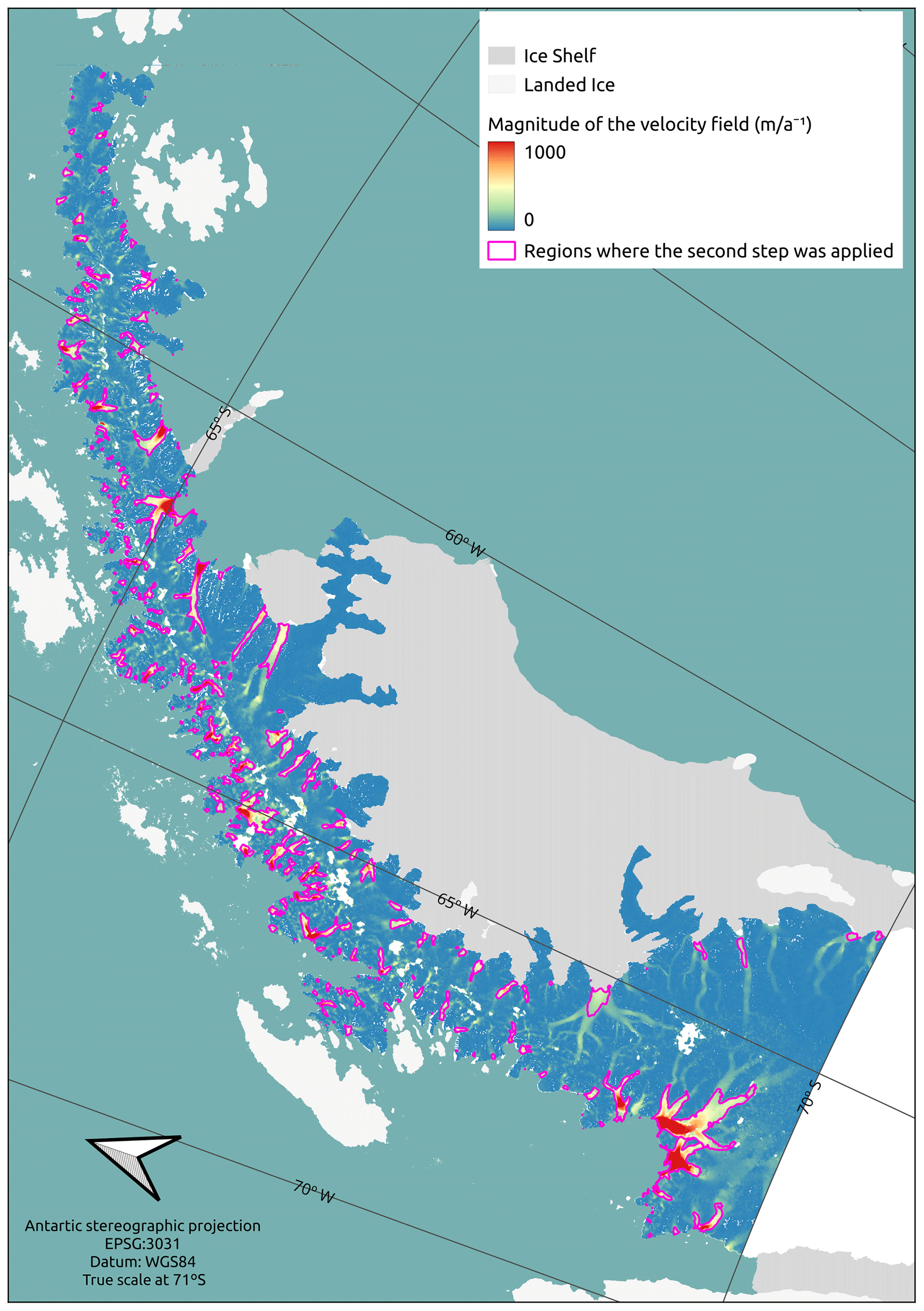
Figure D1 Magnitude of the velocity map (from ENVEO) with the regions where the second step was applied (with $\left|u\right|\ge \mathrm{200}$ m a⁻¹). See Sect. 2 for more information.

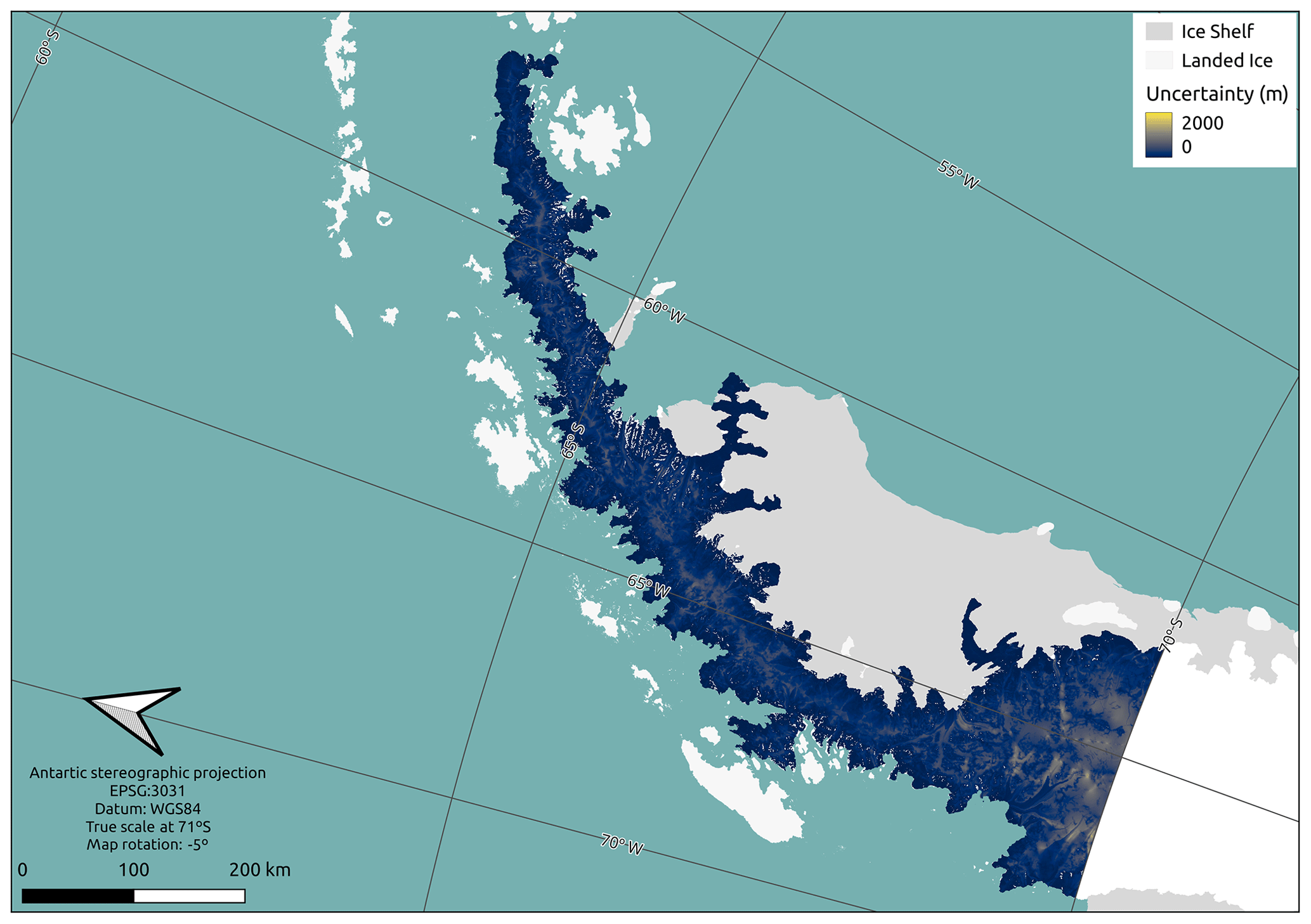
Figure D2 Error map of the two-step approach applied to the ice thickness reconstruction of the Antarctic Peninsula. The method used to calculate the error is presented in Appendix B.

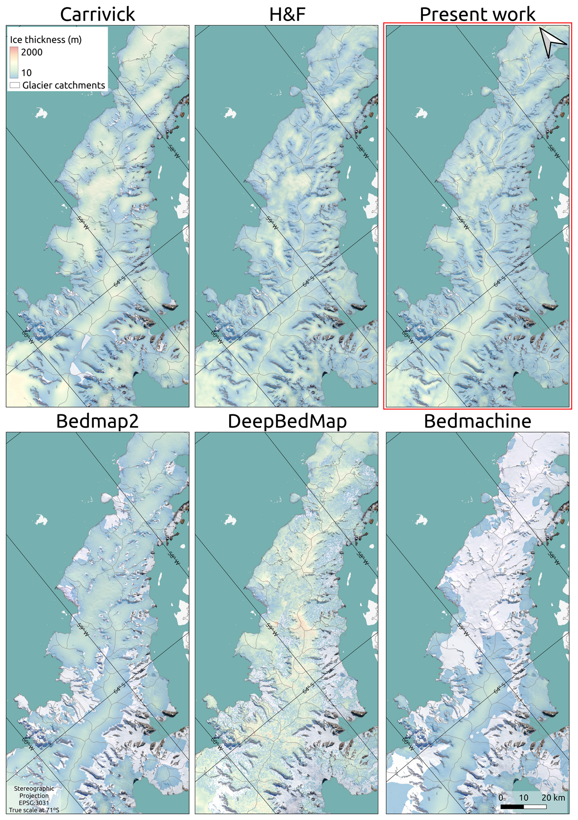
Figure D3 Close-up of the reconstructions of Carrivick, H&F, the present work, Bedmap2, DeepBedMap, and Bedmachine v3, mostly on the Trinity Peninsula. The colors on the ice thickness scale are at 60 % transparency to enable the visualization of the optical image behind (© 2025 TomTom, Earthstar Geographics SIO). We masked ice thickness values lower than 10 m.

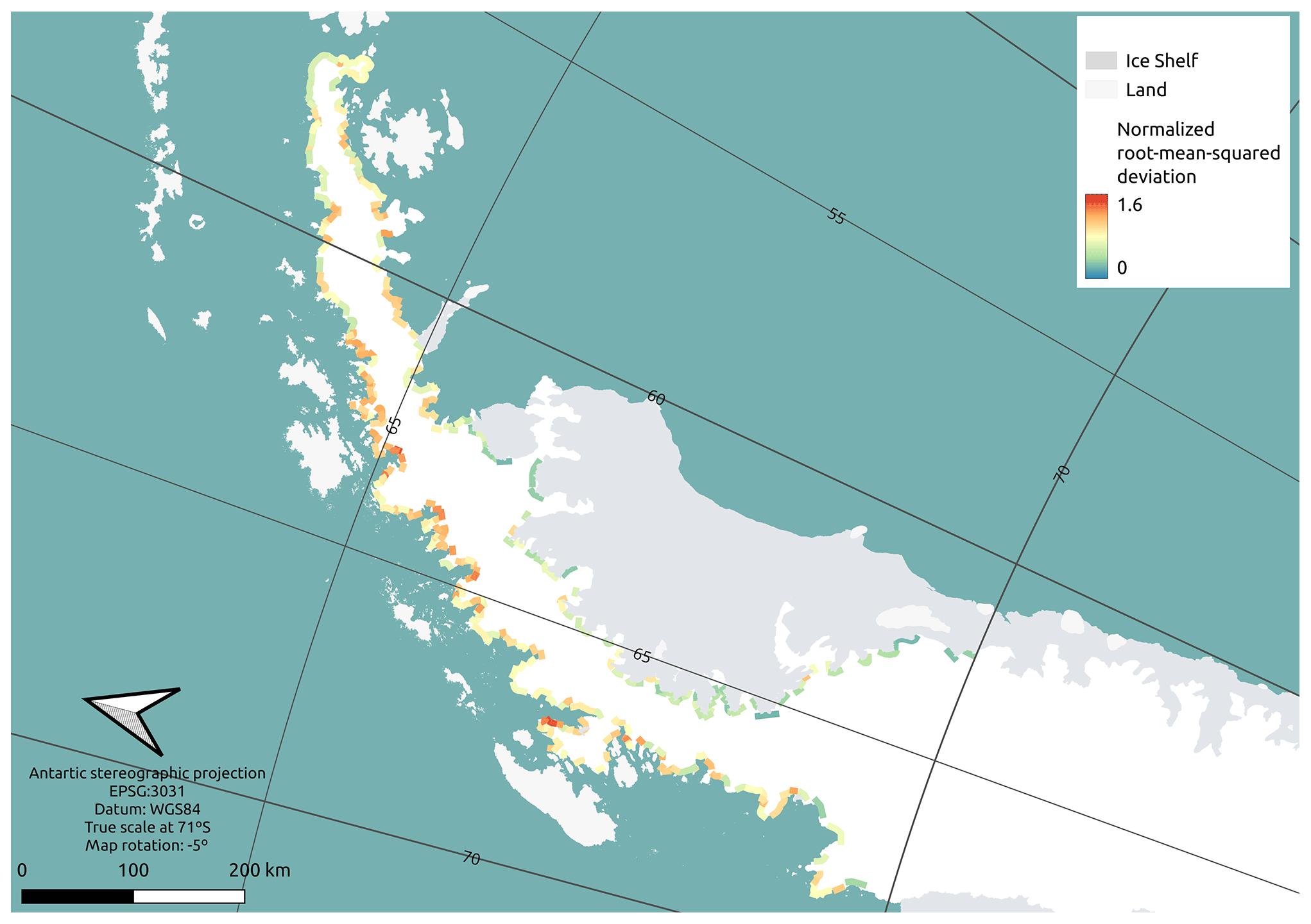
Figure D4 Normalized root-mean-squared deviation (NRMSD) of the six models evaluated in the present work (Carrivick, Huss and Farinotti, the present reconstruction, Bedmap2, DeepBedMap, and Bedmachine v3). See Shahateet et al. (2023) for a complete discussion on NRMSD.

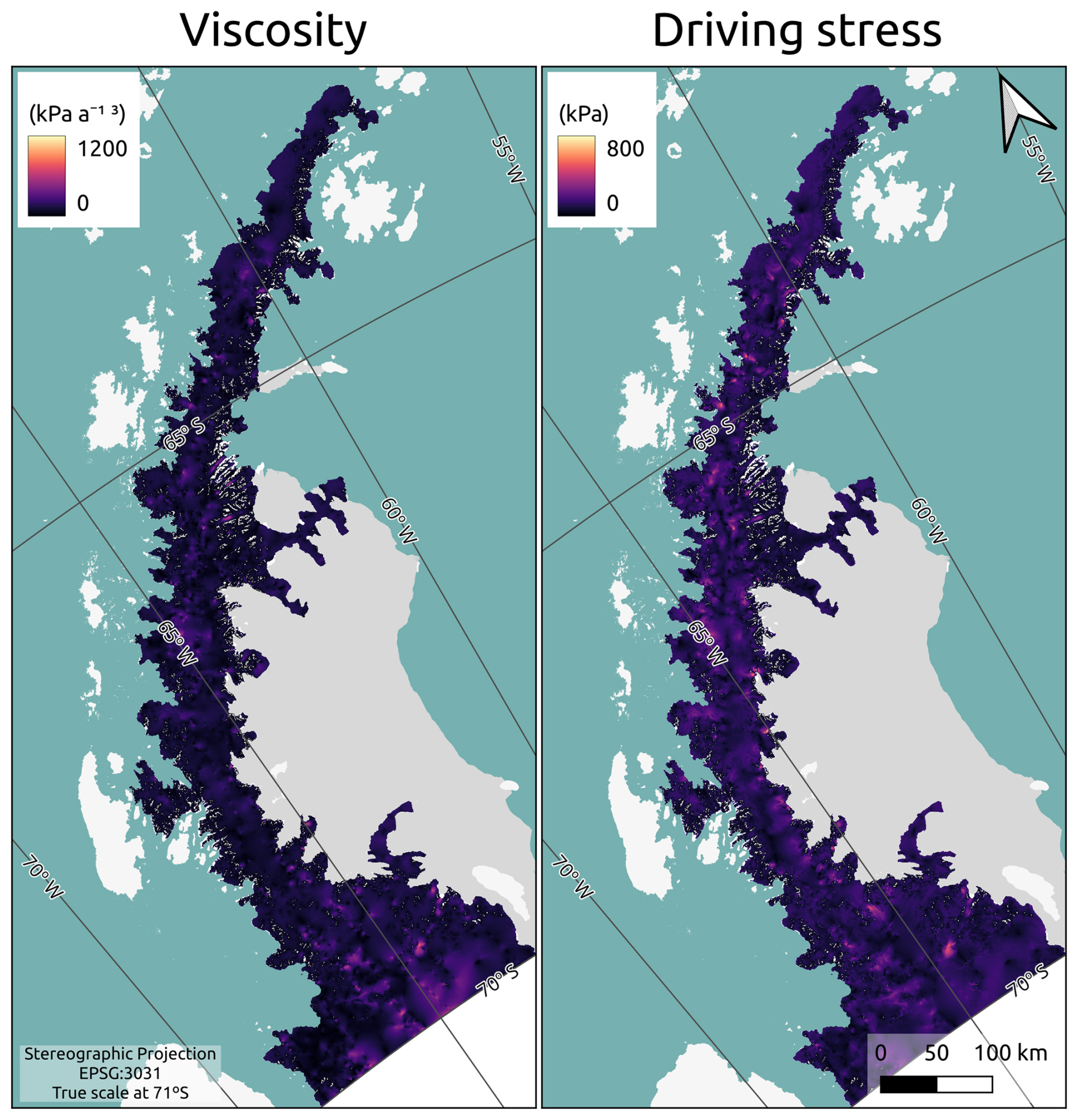
Figure D5 Viscosity (parameter B) and driving stress (τ_d) used to invert ice thickness using shallow-ice approximation and perfect plasticity, respectively.