the Creative Commons Attribution 4.0 License.
the Creative Commons Attribution 4.0 License.
 | 11 Mar 2025
InSAR-derived seasonal subsidence reflects spatial soil moisture patterns in Arctic lowland permafrost regions
Barbara Widhalm
Annett Bartsch
Tazio Strozzi
Nina Jones
Artem Khomutov
Elena Babkina
Marina Leibman
Rustam Khairullin
Mathias Göckede
Helena Bergstedt
Clemens von Baeckmann
Xaver Muri
The identification of spatial soil moisture patterns is of high importance for various applications in high-latitude permafrost regions but challenging with common remote sensing approaches due to high landscape heterogeneity. Seasonal thawing and freezing of near-surface soil lead to subsidence–heave cycles in the presence of ground ice, which exhibit magnitudes of typically less than 10 cm. Our investigations document higher Sentinel-1 InSAR (interferometric synthetic aperture radar) seasonal subsidence rates (calculated per thawing degree days – a measure of seasonal heating) for locations with higher near-surface soil moisture compared to drier ones. Based on this, we demonstrate that the relationship of thawing degree days and subsidence signals can be interpreted to assess spatial variations in soil moisture. A range of challenges, however, need to be addressed. We discuss the implications of using different sources of temperature data for deriving thawing degree days on the results. Atmospheric effects must be considered, as simple spatial filtering can suppress large-scale permafrost-related subsidence signals and lead to the underestimation of displacement values, making Generic Atmospheric Correction Online Service for InSAR (GACOS)-corrected results preferable for the tested sites. Seasonal subsidence rate retrieval which considers these aspects provides a valuable tool for distinguishing between wet and dry landscape features, which is relevant for permafrost degradation monitoring in Arctic lowland permafrost regions. Spatial resolution constraints, however, remain for smaller typical permafrost features which drive wet versus dry conditions such as high- and low-centred polygons.
- Article
(11893 KB) - Full-text XML
-
Supplement
(8596 KB) - BibTeX
- EndNote


Soil moisture information with high spatial resolution is required for numerous applications in Arctic regions. The saturation of soils determines aerobic or anaerobic conditions and consequently carbon or methane release. Therefore, soil wetness representations facilitate the upscaling of fluxes and consequently the determination of greenhouse gas composition (Bartsch et al., 2023; Miner et al., 2022). Additionally, moisture conditions affect soil thermal properties. Wetter soils transfer heat more effectively and rapidly due to higher thermal conductivity and diffusivity (Farouki, 1981). Higher thermal inertia further leads to a quicker response to external temperature changes in wetter soils (Campbell and Norman, 1998). Moreover, wet soils can store more heat for a given temperature change because of higher heat capacity (Campbell and Norman, 1998). Thus, soil moisture data are of high importance in Arctic permafrost regions, especially for permafrost and climate modelling (Subin et al., 2013; Göckede et al., 2017; Zwieback et al., 2019).
Land cover heterogeneity in permafrost lowlands is comparably high with complex spatial patterns of wet and dry soils (Bartsch et al., 2023; Treat et al., 2024). Permafrost-related processes frequently lead to changes in land-surface hydrology. This includes drainage and formation of lakes (Nitze et al., 2017; Jones et al., 2011) and ice-wedge degradation, which can be observed on sub-decadal timescales (Liljedahl et al., 2016). Polygonal features are associated with ice wedges. Polygons are a few metres in diameter and can differ in topography (low centred or high centred), leading to specific wet and dry patterns which change over time (Liljedahl et al., 2016). In general, a change in surface wetness over several years can be associated with permafrost change.
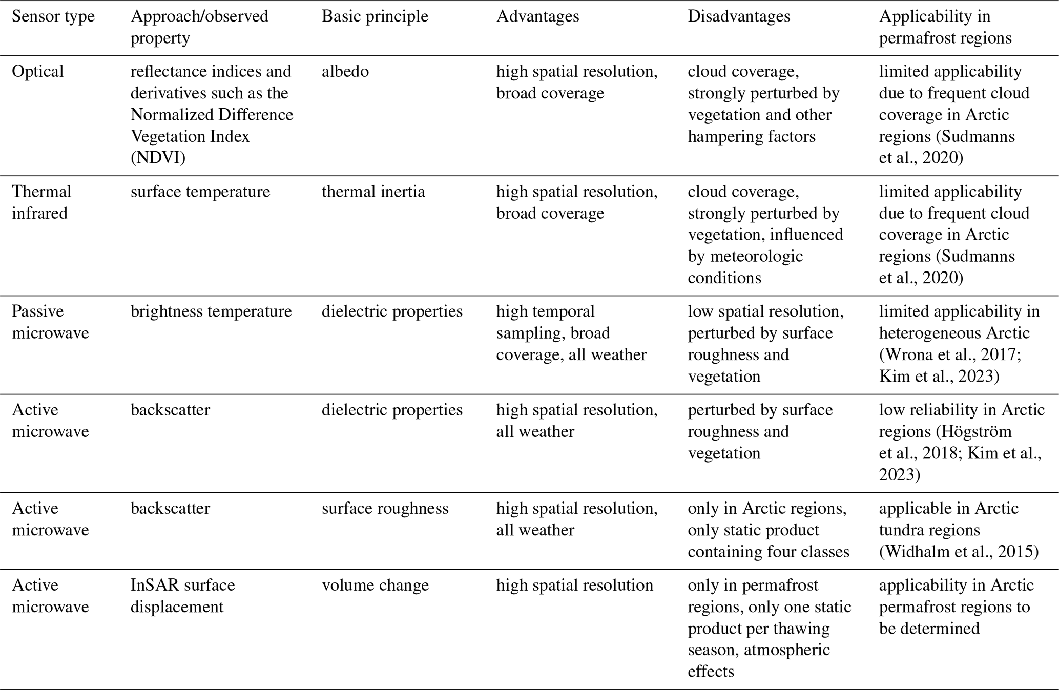
Surface wetness monitoring can be addressed with satellite data, commonly based on data acquired in the microwave domain but also using optical data (Table 1). Thermal observations have also been shown to be of value using the principle of thermal inertia, but their applicability is limited due to frequent cloud cover and the perturbation of meteorological conditions and vegetation (Zhang and Zhou, 2016).
Microwave retrievals make use of the high dielectric permittivity of liquid water in the microwave domain as compared to other soil materials (Barrett et al., 2009). A clear advantage is the ability to penetrate cloud cover, providing the potential for good temporal sampling. For global-scale products, near-surface soil moisture is therefore derived from microwave sensors. However, the used methods which are based on backscatter intensity (scatterometer or synthetic aperture radar) or brightness temperature (radiometers) are of limited applicability in Arctic environments (Wrona et al., 2017; Högström et al., 2018; Kim et al., 2023). The presence of surface water within coarse scatterometer footprints may cause deviations. Wind-induced variations in scattering properties generate biases in lake-rich areas (Högström and Bartsch, 2017). Furthermore, short-term variations in soil moisture derived from C-band radar are influenced by temperature variations in the organic layer (Högström et al., 2018).
For passive microwave sensors, radiative transfer models are applied utilizing the measured brightness temperature, while for active sensors various approaches do exist including change detection and modelling methods (Das and Paul, 2015). Global soil moisture products from active and passive microwave systems like ASCAT (Advanced Scatterometer, C-band; Bartalis et al., 2007; Wagner et al., 2010), AMSR2 (Advanced Microwave Scanning Radiometer 2, multi-frequency; Parinussa et al., 2015; Zhang et al., 2021), SMOS (Soil Moisture and Ocean Salinity, L-band; Kerr et al., 2012; Sadri et al., 2020) and SMAP (Soil Moisture Active Passive, L-band; Colliander et al., 2017; Sadri et al., 2020; Entekhabi et al., 2010) only provide very coarse spatial resolutions (10–50 km) and are therefore not suitable for heterogeneous Arctic landscapes.
As an alternative, higher-resolution (but still comparably coarse) static data (75–500 m) from ENVISAT ASAR data (Advanced Synthetic Aperture Radar, active C-band sensor, horizontal–horizontal (HH) polarization) were used to depict spatial wetness patterns in tundra regions, with winter minimum backscatter values representing surface roughness and serving as a proxy for these patterns (Widhalm et al., 2015). Although fully polarimetric (quad-pol) observations from synthetic aperture radar (SAR) backscatter at the C-band have been shown to be promising (Zwieback and Berg, 2019), these data are usually not acquired. Experiments were made with airborne P-band observations (Ye et al., 2021), but such data are so far not available from space. Recently, Treitz et al. (2024) utilized in situ surface roughness measurements in conjunction with fully polarimetric RADARSAT-2 data to develop a surface roughness model in a localized study. This model, combined with HH-polarized backscatter and local incidence angle data, was subsequently employed to model a time series of volumetric soil moisture.
Interferometric models using SAR data (InSAR) have previously been created to elucidate how changes in dielectric constant, attributed to time-varying soil moisture, affect interferometric phase (De Zan et al., 2014). In recent years, attempts have been made to derive soil moisture changes from related closure phase data (e.g. Michaelides and Zebker, 2020; Wig et al., 2023; De Zan and Gomba, 2018). However, as this requires a triplet of interferograms, with one spanning over all three acquisition dates, this application is not feasible in areas with rapid loss of the degree of interferometric coherence as can be the case in permafrost regions, depending on the used frequency. An alternative method is wetness indices which can be derived from multispectral data. Usually bands with reflectance in the near-infrared and shortwave infrared are used in combination, e.g. for the Normalized Difference Moisture Index (NDMI; Cheţan et al., 2020) or the Tasseled Cap Wetness index (TCW; Frappier et al., 2023), which uses a transformation of multiple visible, near-infrared and shortwave infrared bands. These indices, however, do not give actual volumetric soil moisture content but rather serve as proxies for soil wetness. Although spatial resolution of multispectral data is substantially higher than for global soil moisture products, temporal sampling is limited due to the requirement for cloud-free conditions in frequently cloud-covered Arctic regions (Sudmanns et al., 2020).
Another index that can serve as a proxy for soil moisture is the Topographic Wetness Index (TWI; Riihimäki et al., 2021), which uses topographic information to depict the steady-state soil moisture distribution. This index is, for example, widely used in carbon research (e.g. Mishra and Riley, 2012; Obu et al., 2017; Virkkala et al., 2021). Its applicability as a soil moisture indicator is, however, limited as it solely depends on topographic information, which is merely one component influencing spatial soil moisture patterns (Riihimäki et al., 2021).
InSAR has been already used for a range of permafrost-monitoring applications across the Arctic (Bartsch et al., 2023). Information derived from InSAR is expected to provide insight into active layer and soil properties (Schaefer et al., 2015; Chen et al., 2023; Li et al., 2023). Local InSAR seasonally aggregated subsidence patterns have been reported to be related to wetness gradients (e.g. Liu et al., 2010; Strozzi et al., 2018; Bartsch et al., 2019, 2023). Permafrost regions are characterized by a continuous period of frozen soil conditions. Seasonal phase change occurs with gradual thaw followed by gradual freeze of the so-called active layer. The phase change results in a volume change, depending on the amount of ice/water in the soil. A high subsidence in summer is expected when the water/ice content of the soil is high. Subsidence typically peaks towards the end of the unfrozen period, usually in late August in Arctic permafrost regions. However, the timing of this peak is subject to variability that is influenced by factors such as latitude, local climatic conditions and interannual fluctuations. Consequently, variations in the timing of peak thaw layer thickness might cause it to occur sooner in August or continue into early October. Seasonally aggregated vertical displacement detected by InSAR is of the order of several centimetres (e.g. Strozzi et al., 2018). The magnitude can vary from year to year depending on the warming of the soil or changes in water content through variations in the water budget and is typically less than 10 cm (Streletskiy et al., 2025) but can exceed this in more dynamic regions.
Bartsch et al. (2019) suggested that the temporal evolution of seasonal subsidence reflects differences in soil properties based on vegetation patterns which reflect soil conditions. Scheer et al. (2023) confirmed the linkage to ground ice content, although only a limited number of samples were available. Chen et al. (2020, 2023) suggested the retrieval of equivalent water depth from InSAR subsidence. Seasonally aggregated subsidence may thus hold the potential to serve as a proxy for soil moisture, similar to indices based on multispectral data which represent general land-surface wetness and are available at a similar level of detail (including NDMI from sensors such as Landsat or Sentinel-2).
Temporal resolution is limited to year-to-year changes when data are seasonally aggregated, but is potentially of interest for permafrost-related long-term soil moisture change. Long-term (aggregated over several years) subsidence itself is usually interpreted as a sign for loss of ground ice of the underlying permafrost, as an impact of climate change (e.g. Liu et al., 2015; Wang et al., 2022). Such an approach does, however, require signal stability, and it necessitates an adequate degree of coherence in yearly interferograms to establish connections between data from consecutive years, which can be achieved in areas with limited vegetation growth only (Strozzi et al., 2018).
(Sudmanns et al., 2020)(Sudmanns et al., 2020)(Wrona et al., 2017; Kim et al., 2023)(Högström et al., 2018; Kim et al., 2023)(Widhalm et al., 2015)Table 1Summary of remote sensing techniques for near-surface soil moisture estimation (modified after Engman, 1991; Moran et al., 2004; Wang and Qu, 2009).
One of the major challenges for InSAR applications in Arctic permafrost regions is the limited availability of regular and spatially continuous SAR acquisitions (Bartsch et al., 2023). A second issue is the available wavelength. The longer L-band is less sensitive to vegetation changes and is therefore less prone to coherence loss, allowing longer intervals between acquisitions. Shorter wavelength ranges such as the C-band and X-band are usually only applicable in regions with low vegetation. The X-band is, in general, not freely available, and time series are limited to small regions. With Sentinel-1 A and B, a freely accessible dataset in the C-band range is available and usable for InSAR in Arctic permafrost regions with limited vegetation cover (Sentinel-1A launched in April 2014, Sentinel-1B launched in April 2016 and ended December 2021) (Strozzi et al., 2018). The L-band is currently also mostly acquired on demand across the Arctic; however, usually only one or two acquisitions exist for the unfrozen period, and rarely does any acquisition match the timing of the maximum active layer depth. A general challenge is the impact of snowmelt in spring. Signal decorrelation reduces the availability of image pairs at the time when ground thaw is initiated.
A further obstacle for such an application is atmospheric effects and ionospheric activities which disturb the signal (e.g. Muskett, 2017). When atmospherically contaminated interferograms cannot be simply discarded (as, for example, done in Liu et al., 2010), owing to coherence restrictions, atmospheric corrections are a necessity. Available atmospheric correction methods can be divided into methods with and without external data (Xiao et al., 2021). External data, such as weather reanalysis or global positioning system soundings, can be utilized to mitigate turbulent atmospheric noise from affected interferograms, when sufficiently available (Dini et al., 2019; Jolivet et al., 2014, 2011; Michaelides et al., 2021). Corrections like stacking or time series analysis, which do not rely on external data but rather on data redundancy of interferogram networks, often do not capture the complexity of atmospheric effects (Xiao et al., 2021). On the other hand, methods incorporating external data, like ground observations, satellite observations or numerical weather models, increase processing efforts (Xiao et al., 2021). The Generic Atmospheric Correction Online Service for InSAR (GACOS) tackles this problem by providing easy-to-apply corrections which use external information on atmospheric conditions (Iijima et al., 2021). By incorporating weather model data as well as topographic information, zenith tropospheric delay (ZTD) maps are produced and made available in near real time. The effectiveness of this method has been demonstrated locally (e.g. Murray et al., 2019; Ulma et al., 2021), in some cases, however, with varying degrees of success (e.g. Wang et al., 2019). Particularly, capturing the smaller-scale turbulent atmospheric phase appears to be lacking, while the mitigation of elevation-dependent and long-wavelength components seems to be feasible (Li et al., 2022). The utility of this approach for permafrost applications has not yet been evaluated. This requires testing with in situ data as well as common statistical assessments of phase residuals of the multi-baseline processing. In situ subsidence data are scarce, but the assessment of phase residuals can be applied independently.
An atmospheric correction method frequently applied in permafrost-related studies is spatial filtering, such as high-pass filtering (e.g. Strozzi et al., 2018; Michaelides et al., 2021; Rouyet et al., 2021). This approach is also applicable for InSAR datasets of a daisy-chain network that were processed in series and do not include overlapping interferograms in the time domain. The filtering method relies on the significant disparity in correlation length in the spatial frequency domain of atmospheric and thaw-subsidence-induced effects (kilometre scale compared to metre scale) (Michaelides et al., 2021).
For seasonal aggregation, the timing of acquisitions in summer in relation to the day of year (DOY) presents another difficulty. The driver of ground thaw, the seasonal warming, can be expressed through the sum of positive degree days or degree days of thaw (DDT). Bartsch et al. (2019) suggest the use of DDT to facilitate the comparison of seasonal deformation across different years. Scheer et al. (2023) implemented a DDT-dependent methodology in combination with a normalization step. The approach of DDT requires the availability of temperature data, which are available locally in very few cases only. Therefore, the suitability of reanalyses data needs to be assessed for application across larger regions.
A further challenge is that in situ subsidence measurements as well as soil moisture measurements are scarce across the Arctic, primarily due to logistic constraints (Högström et al., 2018; Strozzi et al., 2018; Bartsch et al., 2019). Spatially distributed measurements are necessary in order to capture landscape heterogeneity, limiting soil moisture measurements to the near surface and mostly to snapshots in time. However, both surface soil moisture and subsidence measurements are available from a long-term monitoring site in central Yamal in western Siberia and in NW Canada. They can potentially serve as reference sites in addition to campaign data.
In summary, the investigation of InSAR-derived aggregated seasonal subsidence rates per DDT as a soil moisture indicator necessitates consideration of various retrieval challenges and assessing the applicability across different permafrost landscape types. Hereafter, all references to subsidence rates refer to the DDT domain.
The purpose of this study is to investigate the potential of seasonally aggregated InSAR subsidence signals for retrieving a soil moisture indicator index. An interpretation scheme of the relationship between DDT and Sentinel-1-based subsidence for soil moisture categories is derived, and its performance is compared to other existing soil moisture approaches using near-surface in situ soil moisture measurements. To ensure reliable results, correcting InSAR values for atmospheric effects is essential. Thus, we assess various methods for correcting these disturbances using in situ subsidence measurements. Regions with varying landscape histories are selected, including sites with relevant in situ measurements and auxiliary measurements.
Three primary study regions with in situ soil property information were investigated within this research (Inuvik in northwestern Canada, central Yamal in northwestern Siberia and Chersky in northeastern Siberia; see Fig. 1 and Table 2). These regions cover permafrost-related long-term monitoring sites. Two of these regions with in situ subsidence measurements and spatially distributed in situ surface soil moisture records were selected for detailed assessment (Inuvik and central Yamal), with one site also offering near-surface as well as borehole temperatures for DDT investigations (central Yamal). Chersky was selected to add to the statistical evaluation of processing results through analyses of the standard deviation of phase residuals. This third region also provides in situ air and borehole temperatures.
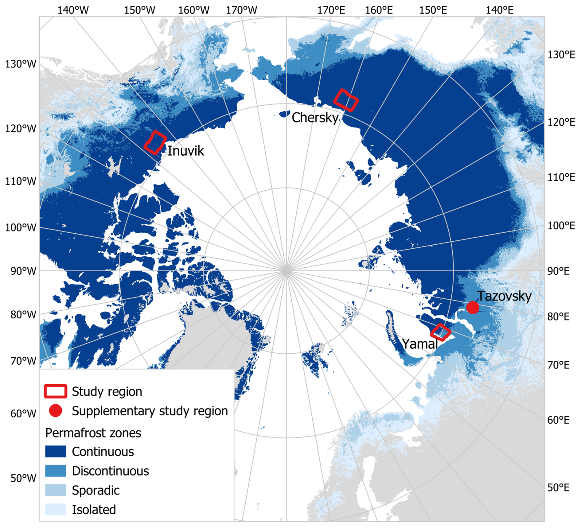
Figure 1Study region locations: Chersky, northeastern Siberia; Inuvik, northwestern Canada; Yamal, northwestern Siberia; and Tazovsky, northwestern Siberia. Background map: permafrost zones (Obu et al., 2019).
The study regions lie in the zone of continuous permafrost, with Yamal also showing areas of discontinuous permafrost in the southwest of the processed scene (permafrost extent data source: Obu et al., 2018). Long-term permafrost monitoring is available in these regions. In northeastern Siberia, the Northeast Science Station (NESS) was established in 1980 near the city of Chersky. The Yamal study region includes the research station Vaskiny Dachi, where permafrost studies have been conducted since 1988 (Leibman et al., 2015). The Trail Valley Creek research station (established in 1991; Pomeroy et al., 1998) is located within the analysed Inuvik region. Various landscape types are represented within the selected regions.
The lake-rich Khalerchinskaya tundra is located northwest of the lower Kolyma River, in the northwest part of the scene of the Chersky area. This region is underlain by ice-poor sands and dominated by a predominantly waterlogged landscape (Fyodorov-Davydov et al., 2004). The river valley is characterized by alluvial deposits (Shmelev et al., 2017) and features regularly flooded shrub and herbaceous vegetation (JRC, 2003). The east and south of the scene are partly underlain by organic- and ice-rich Yedoma deposits (Grosse et al., 2013), featuring needle-leaved and deciduous tree cover as well as herbaceous land cover on mountain regions (JRC, 2003).
The Yamal area is characterized by marine, coastal-marine and fluvial-marine lithologies (Leibman et al., 2015), where shrub and herbaceous tundra dominates (Khitun and Rebristaya, 1998; Widhalm et al., 2017a; Stolbovoi and McCallum, 2002).
The Mackenzie delta area of the Inuvik region is covered by needle-leaved evergreen trees (JRC, 2003) and is characterized by alluvial sediments (Geological Survey of Canada, 2014). The west of the scene is dominated by shrub cover and sparsely herbaceous and shrub-covered mountains (JRC, 2003). To the west and east of the delta, glacial sediments prevail (Geological Survey of Canada, 2014). East of the delta, the land cover is dominated by a mosaic of tree cover and other natural vegetation with areas of shrub and herbaceous cover (Bartholomé and Belward, 2005; JRC, 2003).
In order to support the discussion on the applicability of InSAR for permafrost-related features prone to degradation, a fourth region was investigated in an area of discontinuous permafrost near the Tazovsky settlement, about 500 km southeast of the Yamal sites. The characteristics of polygonal tundra, which may vary in moisture regimes, are discussed, highlighting the relevance of InSAR results for characterizing different types of permafrost wetlands. This region is characterized by a relatively flat, slightly dissected surface with a high number of wetlands, lakes and widely spread flat-topped and convex, hummocky peatlands (Babkin et al., 2018). The temperature of permafrost ranges from 0 to –1.0 °C, decreasing to –1.5 °C in dome-shaped peatlands (Koroleva et al., 2021). Polygonal features are widespread in this area and are usually linked to peatlands (Khomutov et al., 2022). The features include high- and low-centred polygons. Low-centred polygons have comparably wet soils and/or water-filled ponds inside them. Further landscape features include watery troughs on peatlands, over-saturated wetlands and wetlands without visible polygons.
The active layer thickness (maximum thaw depth; source: ESA Permafrost_cci, year 2019 of Obu et al., 2021) is largest for the Inuvik study region and the region around Tazovsky with values of, on average, 0.96 and 0.94 m, respectively. Yamal shows average active layer thickness values of 0.84 m, and the Chersky area features the thinnest active layers with values of circa 0.64 m.
3.1 Sentinel-1
ESA's Sentinel-1 satellites are operating C-band SAR instruments with wavelengths of 5.6 cm. For our investigations, we used single look complex (SLC) images in interferometric wide (IW) swath mode, which provide a ground sampling distance of 2.3 m in range and 13.9 m in azimuth direction as well as a swath width of 250 km. Sentinel-1A was launched in April 2014 and Sentinel-1B followed in April 2016. The constellation of two satellites offered a possible repeat cycle of 6 d; however, due to global acquisition strategies, 12 d was more common and was also generally available for most Arctic regions. Regular acquisitions started for most study regions in mid-2016, not always covering the entire thawing season of this year. At the end of 2021, Sentinel-1B stopped operating, resulting in no recent Sentinel-1 data acquisitions for the Siberian study regions. Table S1 in the Supplement indicates the acquisition dates of all Sentinel-1 SAR acquisitions used in this study. Paths and frames of the investigated scenes can be found in Table S2 in the Supplement. The seasonal study periods were selected from the start of the thawing season, as soon as interferograms showed good coherence, until the onset of freezing (delineated from ERA5 reanalysis data).
3.2 In situ data
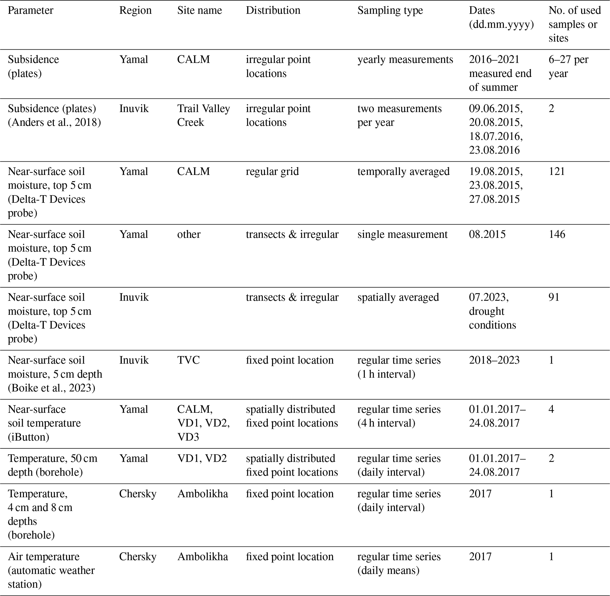
In situ data, including subsidence, soil moisture and temperature measurements, were available for the three study regions. An overview of the used data is provided in Table 2.
3.2.1 Yamal
Yearly in situ subsidence measurements were conducted at the CALM (Circumpolar Active Layer Monitoring) grid near the research station Vaskiny Dachi in central Yamal. For this, L-shaped metal rods were inserted through holes in plates to the base of the active layer, with the hooked end tight on the plate. In winter, frost heave raises the plate, pushing the rod up, where it becomes fixed by freezing. During spring thaw, the plate subsides with the ground surface, while the rod remains fixed. The difference between the plate and the rod's end is measured as ground movement. Surface subsidence measurements started in 2016 with five to six points. An additional 20 points are available since 2018 and a further 4 points since 2021. Measurements were performed yearly at the end of August or start of September with the exception of 2016 when travel restrictions resulted in measurements not until mid-October. The CALM grid is situated on a sloping plain where dry cryptogram crust dominates the flatter upper part. Grasses and mosses as well as low and high shrubs can also be found in the remaining parts along with patches of wet sedge (Widhalm et al., 2017a).
Soil moisture measurements were conducted at the 121 CALM grid points (Widhalm et al., 2017b) and at seven transects containing 12 to 34 individual points, as well as at 10 selected additional locations. Moisture values were measured at the top 5 cm with the Delta-T Devices HH2 soil moisture sensor. For the soil moisture values at the CALM grid, measurements of three different dates in August 2015 were averaged. The other points were measured only once, also in August 2015. The moisture conditions in the Yamal Peninsula study region were normal in 2015, with total precipitation values of 185 mm for the months of June through September, compared to median values of 188 mm over a 15-year period (measured at Maresale). Precipitation values during the years of InSAR observations ranged from 120 mm in 2017 to 244 mm in 2021. For the comparison with InSAR results, soil moisture values of points which were located within the same Sentinel-1 pixel were averaged. This resulted in 132 samples (68 CALM grid values, consisting of 121 valid samples, and 64 pixels in the other categories, containing 146 valid measurements).
Near-surface soil temperatures for the derivation of DDTs based on in situ data were measured with DS1921G-F5 Thermochron iButton devices between October 2016 and August 2017. Temperatures were recorded at four sites at the Yamal study region (locations shown in Fig. 2). One point is located at the CALM grid, while the other three points are placed at monitoring sites which were established within the Greening of the Arctic (GOA) project of the International Polar Year (IPY) (Walker et al., 2009). Site VD1 is located on a gentle terraced hilltop with clayey soils, sedge and dwarf-shrub, and moss tundra. VD2 is on a broad hilltop, characterized by sandy and clayey soils dominated by dwarf-shrub, graminoid and moss tundra. Site VD3 is characterized by dry dwarf-shrub–lichen tundra on sandy soils (Walker et al., 2009).
Additionally, borehole temperature data at 50 cm depth of two of the GOA points (VD1 and VD2) were used.
3.2.2 Chersky
Borehole data from depths of 4 and 8 cm, as well as temperature data from an automatic weather station near the borehole located approximately 15 km south of the city of Chersky at the research site Ambolikha, were utilized. This site is located on the floodplain of the Kolyma River and dominated by wet tussock tundra with tussock-forming sedges and cotton grasses on an organic peat layer overlain by alluvial mineral soils (Göckede et al., 2019).
3.2.3 Inuvik
At the Inuvik study site, in situ soil moisture measurements were conducted similarly to those in Yamal, using a Delta-T Devices HH2 soil moisture sensor in the top 5 cm. The measurements were conducted in the region between north of the city of Inuvik and south of the Trail Valley Creek research station in July 2023. As this time was characterized by drought conditions, the maximum of multiple samplings was further used at each measurement point. The measurement points were recorded in transects and irregular point locations. Again, samples within the same InSAR pixel were averaged for comparisons with InSAR results; 78 pixels were used including 91 measuring points.
To investigate the effects of soil moisture change on InSAR results, soil moisture time series at Trail Valley Creek from Boike et al. (2023) were analysed. Soil moisture data at a depth of 5 cm for the years 2018–2022 were used.
In situ subsidence data were available from Anders et al. (2018) for the years 2015 and 2016. Similar to the measurements in Yamal, poles were anchored below the active layer. Measurements were performed twice per year, recording the distance between the top of the pole and a plate on the surface.
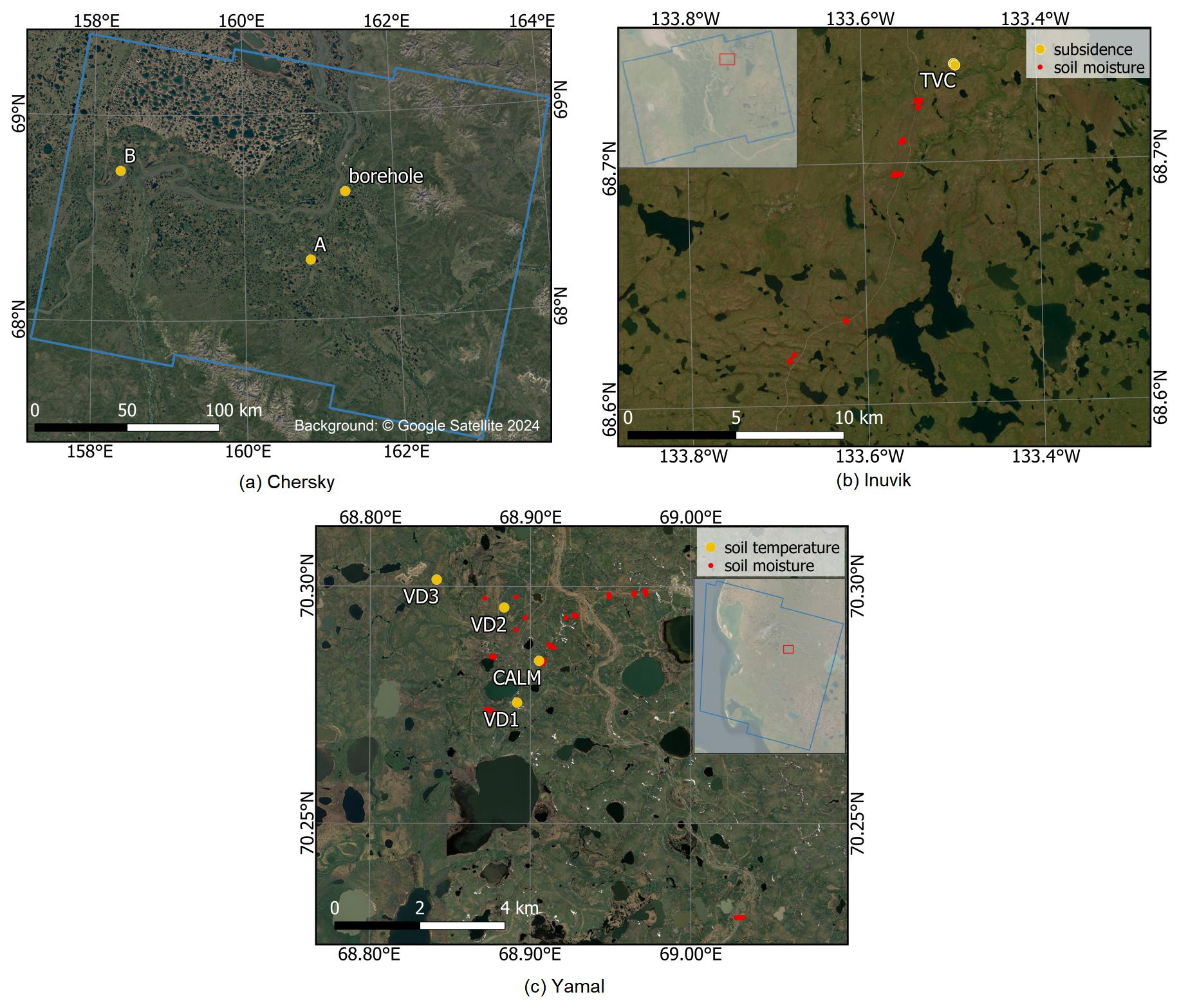
Figure 2Sample point and in situ data locations (see also Table 2 for the in situ data description overview). (a) Chersky region: sample points for time series plots (without in situ information) and borehole location (Background map data source: Google Satellite). (b) Inuvik region: locations of in situ near-surface soil moisture measurements and in situ subsidence data (Background map data source: Esri Satellite). (c) Yamal region: locations of in situ near-surface soil temperature and soil moisture measurements (Background map data source: Esri Satellite). Panels (b) and (c) only show a subset of the processed region, depicting the area where in situ data are available.
3.3 Auxiliary data
Air temperature, utilized for deriving DDT values across the entire study regions, was derived from ERA5 reanalysis data. ERA5 combines model information with observations to produce a globally consistent dataset (Hersbach et al., 2023). We used air temperature at 2 m above the surface at a temporal resolution of 2 h at 0.25° spatial resolution.
Landsat 8 (Earth Resources Observation and Science (EROS) Center, 2020) Level-2 (bottom of atmosphere) data (30 m spatial resolution) were acquired for the derivation of NDMI, which utilizes bands in the near-infrared and shortwave infrared parts of the spectrum to depict changes in water content of leaves. Dates were selected close to the in situ soil moisture sampling dates, specifically on 10 August 2015 for Yamal and on 6 July 2023 for Inuvik.
For the calculation of TWI, the ArcticDEM (Porter et al., 2022) at 2 m spatial resolution was utilized, which is delineated from optical stereo imagery.
ESA's CCI soil moisture product (Gruber et al., 2019; Dorigo et al., 2017, 2023; Preimesberger et al., 2021) was used for evaluation purposes. This daily, global soil moisture product, at 0.25° spatial resolution, combines various active and passive microwave products. Here, we utilized the passive microwave and combined (active and passive) product, which are provided in volumetric soil moisture units.
High-resolution satellite imagery of QuickBird-2, WorldView-2 and WorldView-3 (Khairullin et al., 2019), topographic surveys (Babkin et al., 2018), and unoccupied aerial vehicle (UAV) images were available for the area surrounding the Tazovsky settlement. The UAV images, acquired in 2022, covered an area of about 25 km2. Additionally, high-resolution satellite images available via Google and Esri Satellite maps were used in the proximity.
The Generic Atmospheric Correction Online Service for InSAR (GACOS; Yu et al., 2018) was developed at Newcastle University and provides high-spatial-resolution zenith tropospheric delay (ZTD) maps based on numerical weather models. Surface pressure, temperature and specific humidity are from a high-resolution ECMWF weather model at 0.1°, and 6 h resolutions are used as input as well as the 90 m resolution Shuttle Radar Topography Mission (SRTM) DEM (60° S–60° N) and the Advanced Spaceborne Thermal Emission and Reflection Radiometer (ASTER) Global Digital Elevation Model (GDEM) (at higher latitudes). An iterative tropospheric decomposition model (Yu et al., 2017) was implemented in order to separate the stratified and turbulent components from the tropospheric delays and produce ZTD maps, which are globally available in near real time.
The described method is based on seasonal freezing and thawing of the active layer in permafrost regions. In the presence of ice in the ground, the surface subsides throughout the thawing season. This can be measured using InSAR. Bartsch et al. (2019) demonstrated that the displacement values follow a nearly linear progression with respect to DDT. Alternatively, a dependency on has been employed in several previous studies (e.g. Liu et al., 2012; Hu et al., 2018). An overview of the major processing steps is given in Fig. 3. We utilize this relationship in order to link satellite data to in situ near-surface soil moisture, which was collected for calibration and validation purposes. Special attention is paid to interfering atmospheric effects, by testing various correction methods.
InSAR displacement results and atmospheric correction performance are evaluated by investigating displacement time series at sample point locations across all study regions. A comparison to in situ subsidence data is performed for the Yamal site, and standard deviations of phase residuals are compared for unfiltered and GACOS-corrected results across all study regions.
GACOS-corrected results and comparable soil moisture indices are evaluated against in situ soil moisture measurements of Yamal and Inuvik. While in situ soil moisture measurements were limited to the top 5 cm, we posit that under typical conditions they are representative of the entire active layer, which can be measured using InSAR. An empirical relationship between GACOS-corrected results and in situ soil moisture of Yamal calibration data (normal moisture conditions) is derived and its quality compared to the CCI soil moisture product. An overview of the conducted evaluations is provided in Table 3.
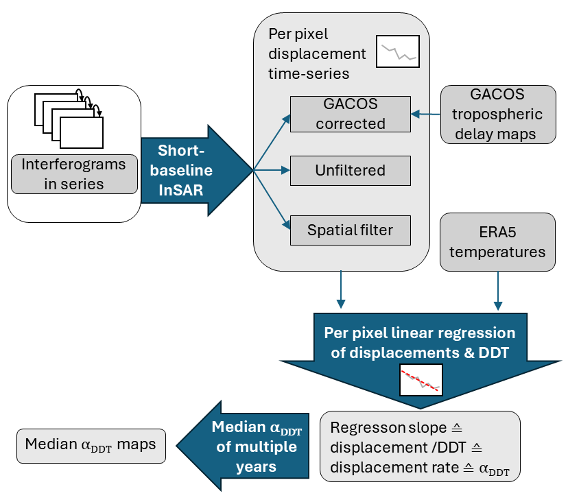
Figure 3Overview of the workflow used for the derivation of median surface displacements in the degree day of thaw (DDT) domain (αDDT).
Table 3Evaluation and comparison of atmospheric correction and soil moisture indices across various study regions.
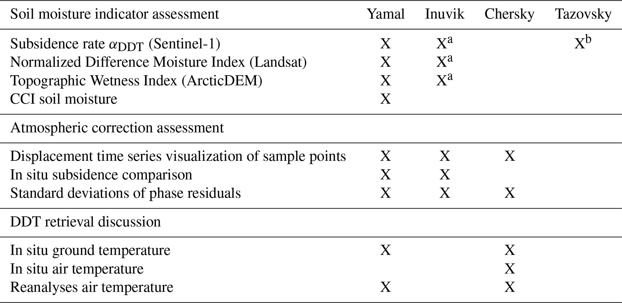
a In situ soil moisture measurements represent drought conditions; b permafrost polygonal features' spatial distribution.
4.1 InSAR processing
Our InSAR processing sequence largely follows the workflow outlined by Strozzi et al. (2018). This includes the application of precise orbit files, co-registration and computation of interferograms with a multi-looking factor of 5 by 1 pixels. The interferograms were processed in series in a daisy-chain network. Longer time steps which would result in temporally overlapping interferograms were often not possible due to a decrease in coherence. Temporal baselines were therefore mostly 12 d, in some cases also 24 or even 36 d, when acquisitions were missing or due to apparent co-registration errors or heavy influence of a turbulent atmosphere, which lead to the exclusion of isolated acquisitions. Perpendicular baselines were on average 46 m, with a maximum value of 152 m. The next processing steps comprise topographic phase removal, incorporating the Copernicus DEM (European Space Agency, 2021) with 30 m spatial resolution, adaptive phase filtering (Goldstein and Werner, 1998), phase unwrapping (Costantini, 1998), and calculation of vertical displacements via short-baseline InSAR (Berardino et al., 2002) (assuming that all the displacement is vertical) and terrain-corrected geocoding. The assumption of only vertical displacements holds true for the investigated in situ site locations where only low slopes were being observed, and horizontal displacements caused by mass movements, such as solifluction, can be ruled out. Areas with slopes of >5° were subsequently masked to ensure the validity of this assumption. Reference points were selected at or close to airstrips in Inuvik (bedrock outcrop 6 km southeast of the airstrip), Chersky and Bovanenkovo (Yamal region). Areas of low coherence were masked out (average coherence <0.8 and average coherence of filtered interferograms <0.5).
Opting for a daisy-chain network reduces atmospheric effects for the difference between the first and last scenes, which is an advantage of this processing method. However, this approach also increases noise in the integration, including that related to soil moisture changes. The use of a daisy-chain network makes it challenging to distinguish between surface deformations and atmospheric effects. These atmospheric artefacts, along with phase delays possibly arising from soil moisture changes (which are considered a possible limitation and will be discussed later), can introduce noise and inaccuracies into the interferometric phase, leading to errors in the estimated deformation signals. Therefore, two different compensation methods for atmospheric effects were tested. First, a spatial filter of the linear-least-squares type, as implemented in the GAMMA software, was applied to the displacement maps. Different filter radii were assessed. Secondly, GACOS corrections were applied on unwrapped interferograms. Artefacts were encountered in the GACOS products for some study regions (Fig. S1 in the Supplement), stemming from the ASTER DEM for areas north of 60° N used by the provider (Yu et al., 2018). The data provider offers the possibility to send in an alternative DEM for a requested area. However, in this case we opted for correcting the GACOS files by masking out the artefacts and filling in the missing values with the median of a moving window.
4.2 DDT and subsidence relationship
The data gap at the beginning of the thawing season, caused by low coherence values due to snow cover on the ground, was accounted for by extrapolating the time series using linear regression (Bartsch et al., 2019). This ensured that every depicted seasonal displacement time series starts with the onset of thaw at DDT = 0. The displacement values calculated for the comparison to in situ data were then offset using the slope of the regression of the displacement time series. Utilizing the assumed linear relation between DDT and seasonal surface subsidence, we derived the subsidence rate (displacement per DDT, hereinafter referred to as αDDT) at each pixel (Eq. 1), reversing the sign in the equation to produce higher positive values for areas with higher soil moisture.
where di represents the total displacement between the first acquisition and time step i, and n represents the maximum number of available dates.
Using αDDT allows for a calculation of displacement indices that are independent of acquisition time. However, it should be noted that subsidence may precede at a faster rate at the non-captured beginning of the thawing season compared to the later season (Schaefer et al., 2015). This can introduce a potential source of error. Therefore, as an alternative approach, was tested, incorporating a dependency on (Liu et al., 2012; Hu et al., 2018; Liu, 2024). The DDT was derived from the mean air temperature at 2 m height of daily averaged ERA5 data with a coarse spatial resolution of 0.25°, which might introduce a source of uncertainty compared to the higher resolution of Sentinel-1 data. We calculated αDDT for each thawing season. In order to derive general displacement patterns, we calculated the median αDDT values of all processed years. Using the median value aids mitigating the effect of remaining atmospheric disturbances within some of the processed years. The median αDDT was further used to investigate the relationship of InSAR surface displacement signals and soil moisture conditions.
4.3 Validation
In order to quantify the validity of InSAR measurements for soil moisture retrieval, the in situ near-surface soil moisture dataset of Yamal was split into calibration and validation datasets. For validation purposes, the data from Yamal were exclusively selected due to their acquisition during typical moisture conditions, in contrast to the data from Inuvik, which were acquired during drought conditions. To address the high heterogeneity of soil moisture patterns and to deal with differences in scale and geolocation of in situ compared to InSAR data, the in situ records were grouped into discrete bins representing 10 % volumetric soil moisture increments (comparable to Bartsch et al., 2020). Median αDDT values were then computed for each bin within the calibration dataset to establish a linear relationship and compared to the results derived using from the alternative approach. The coefficient of determination (R2) was calculated to quantify the strength of this relationship, while P values were derived to ascertain its statistical significance. Additionally, the root mean square error (RMSE) was determined for the validation dataset to evaluate predictive accuracy. Additionally, classification accuracy was assessed for classifications comprising a total of six or three moisture level classes. To achieve this, the αDDT values of samples from the validation dataset were converted into moisture values using the established linear relationship. Subsequently, these values were categorized into distinct moisture levels and compared to the true moisture classes.
4.4 Processing of auxiliary data
To assess the performance of αDDT as a moisture indicator, other indices such as NDMI and TWI were also compared. The NDMI was calculated for the Inuvik and Yamal sites, where in situ near-surface soil moisture measurements were available, using bands 5 and 6 of the Level-2 (bottom of atmosphere) Landsat 8 data (Eq. 2).
The TWI is defined as
with SCA being the specific catchment area, and ϕ being the slope angle. The ArcticDEM at 2 m spatial resolution was used for its calculation.
For the discussion of the results in the context of permafrost-specific landscape features, different land-cover units were manually digitized based on UAV observations, high-resolution satellite images, and the online services of Google and Esri Satellite maps. Areas of high- and low-centred polygons were differentiated from other tundra (with and without wetlands) for 25 selected areas, each sized 1 km × 1 km. The average usage of different types of remote sensing data was 15 % from UAV images, 77 % from high-resolution satellite images and 8 % from online services. The average fraction of area covered by low-centred polygons is 3.9 % (ranging from 0.4 % to 11.2 %). High-centred polygons cover a larger average fraction of about 12 % (ranging from 4.4 % to 29.0 %).
5.1 Atmospheric correction
5.1.1 Spatial filter radius for InSAR processing
In order to specify the filter radius, some initial tests were performed and visually evaluated. Figure S2 in the Supplement depicts results of a displacement map with no applied filter, a spatial filter of radius ∼ 60 km and of radius 6 km. While atmospheric effects are still clearly noticeable for the 60 km radius, they were mostly removed for the 6 km radius. Although it cannot be excluded that large-scale deformation signals have also been removed, a radius of about 6 km (512 pixels) was chosen for further investigations.
5.1.2 Displacement time series – Chersky, Yamal and Inuvik
To investigate temporal InSAR subsidence results, we examined the displacement time series for selected sample points.
The points for Chersky were selected within an eastern and western part of the Sentinel-1 scene. They are located in areas of similar land cover within wet ecotopes, where summer subsidence can be expected (locations are shown in Fig. 2). They represent different patterns of tropospheric delay (e.g. Fig. S1 in the Supplement). While the differences at point A are not as pronounced for unfiltered and GACOS-corrected results, point B shows clear improvements with GACOS correction (Fig. A2). The implausible heave signal observed during the thawing seasons of the years 2017 and 2018 in the unfiltered results was mostly corrected when the GACOS correction was applied. However, as illustrated in Fig. A1, this heave signal was not corrected everywhere. This might be attributed to unfiltered atmospheric effects, or, as similar patterns were observed in two different years, displacements at the reference point cannot be ruled out. Unfiltered and GACOS-corrected results exhibit distinct temporal fluctuations, whereas spatially filtered results are clearly smoothed. However, this smoothing also results in a reduction of overall magnitude of displacement values.
For the Yamal region, the displacement time series is investigated for a long-term in situ subsidence point on the CALM grid (Fig. A3). While unfiltered and GACOS-corrected time series are very similar, spatially filtered data exhibit the same smoothing and reduction in subsidence magnitude as in the Chersky example. The depicted sample point, which exhibits an average subsidence of 3 cm, falls within the mean range of other points measured on the CALM grid, with a mean subsidence of 4.7 cm ± 2 cm (standard deviation). The agreement with in situ subsidence values may vary with sample location, which is further investigated in the next section.
In situ subsidence values for the Inuvik region were available for different years than InSAR data but were nonetheless used to compare general magnitudes (Fig. A4). In situ values were extrapolated similarly to InSAR data to account for the data gap between the first measurement and the start of the thawing season. The in situ subsidence rates of 2015 matched well with InSAR data in terms of magnitudes. Higher rates, such as those observed in 2016, were also recorded with InSAR for the year 2023, particularly for point TVC1. However, for the spatially filtered results, the magnitude for 2023 at TVC1 was reduced. GACOS was able to correct for some of the fluctuations in the unfiltered results; however, in the case of 2019, it introduced additional artefacts. Comparison of GACOS results in the domain (Fig. S3 in the Supplement) shows that the in situ data align more closely with the results in the DDT domain.
5.1.3 In situ subsidence comparison – Yamal
The results of the InSAR time series were evaluated with in situ subsidence measurements at the CALM grid (Fig. 2) in Yamal (Bartsch et al., 2019). Results for the years 2016, 2017, 2018 and 2021 were compared (Fig. 4). For the year 2019, there were mostly no Sentinel-1 data available for this region, and in 2020 missing acquisitions resulted in low coherence values preventing the generation of reliable results. The number of available in situ points was extended over the years, and some points exhibit data gaps; however, for the 2D boxplots of in situ and InSAR values, all available data points were included, along with an indication of the number of available samples (Fig. 4). While unfiltered and GACOS-corrected plots show similar results, the spatially filtered results deviate and feature lower values, even heave, especially for the year 2016. All methods (unfiltered, GACOS-corrected, spatial filtering) exhibit lower annual mean InSAR subsidence signal values across all points with the longest available in situ time series compared to in situ measured values (Fig. 4 bottom right). The lowest match to in situ values was derived for the spatially filtered results. The range of InSAR values is roughly similar for unfiltered and GACOS-corrected results for these points; however, while unfiltered values seem to disperse, GACOS-corrected values are less scattered.
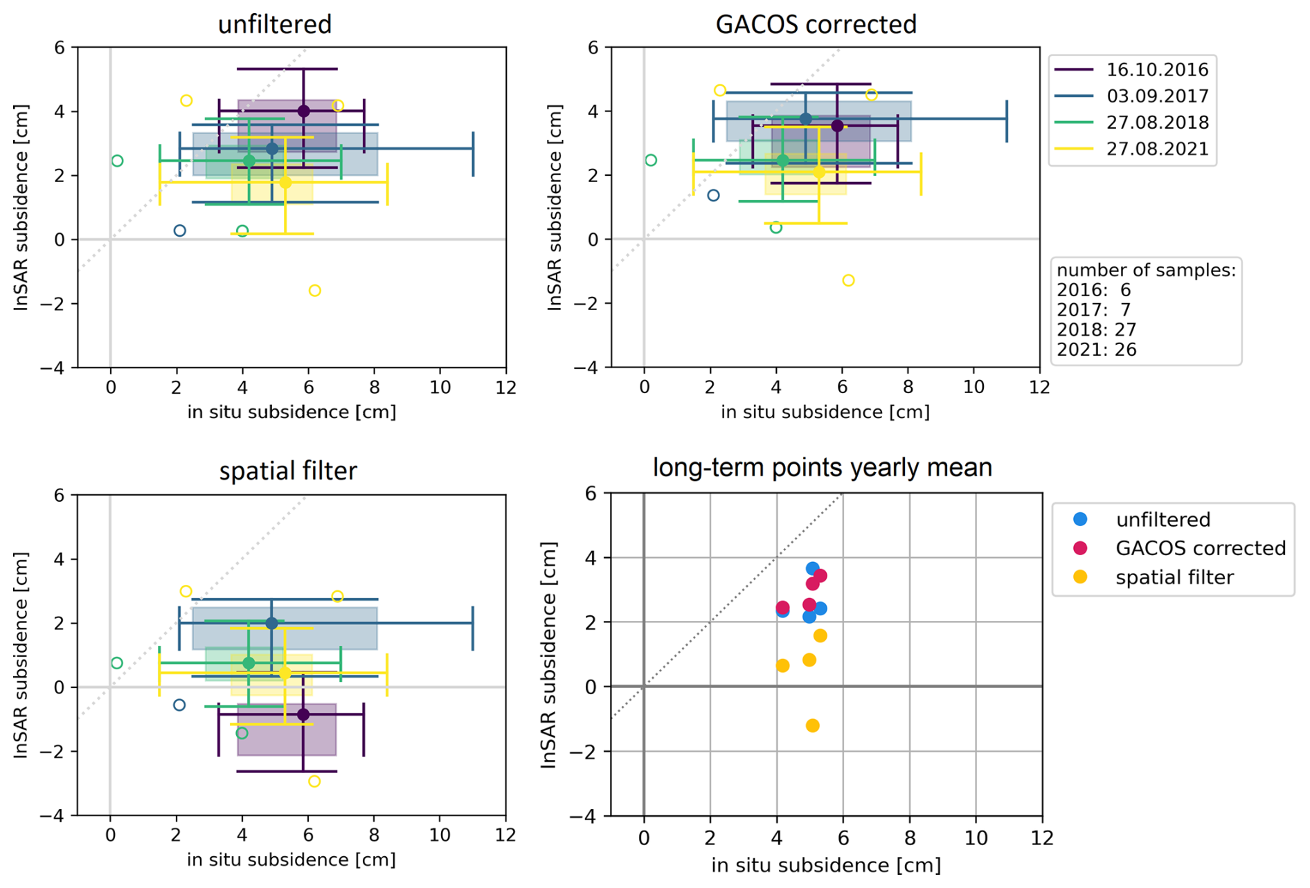
Figure 4The 2D boxplots (depicting median values – filled circles; quartiles – boxes; minima and maxima – whiskers; and outliers – empty circles) for in situ subsidence measured at the CALM grid in Yamal vs. InSAR subsidence for all available points per year (note the available number of samples varying per year, indicated in the box on the right-hand side). Lower right: scatterplot of mean subsidence values for six long-term sample points (measured in 3–4 years) for each method and all available years (each point representing 1 year).
5.1.4 Standard deviation of phase residuals for all regions
Focusing on the GACOS-corrected results, the standard deviations of the phase residuals are further investigated in comparison to unfiltered results (Fig. 5). The phase residuals are derived through a comparison between simulated interferograms of a smoothed time series and the actual interferograms. Due to the absence of redundancy within the interferograms, the resulting values primarily reflect the effects of the time series smoothing. The statistics for the whole processed scenes for each thawing season were investigated, with terrain slopes of >5° being masked out in order to exclude αDDT values which may encounter erroneous results for vertical subsidence due to additional horizontal displacement resulting from mass movements, such as solifluction. The values improve for the GACOS-corrected results (see Fig. 5 and also Fig. A7, depicting differences between unfiltered and GACOS-corrected results), especially for the Chersky and Inuvik regions. However, for the Yamal region most years showed better values before the GACOS correction.
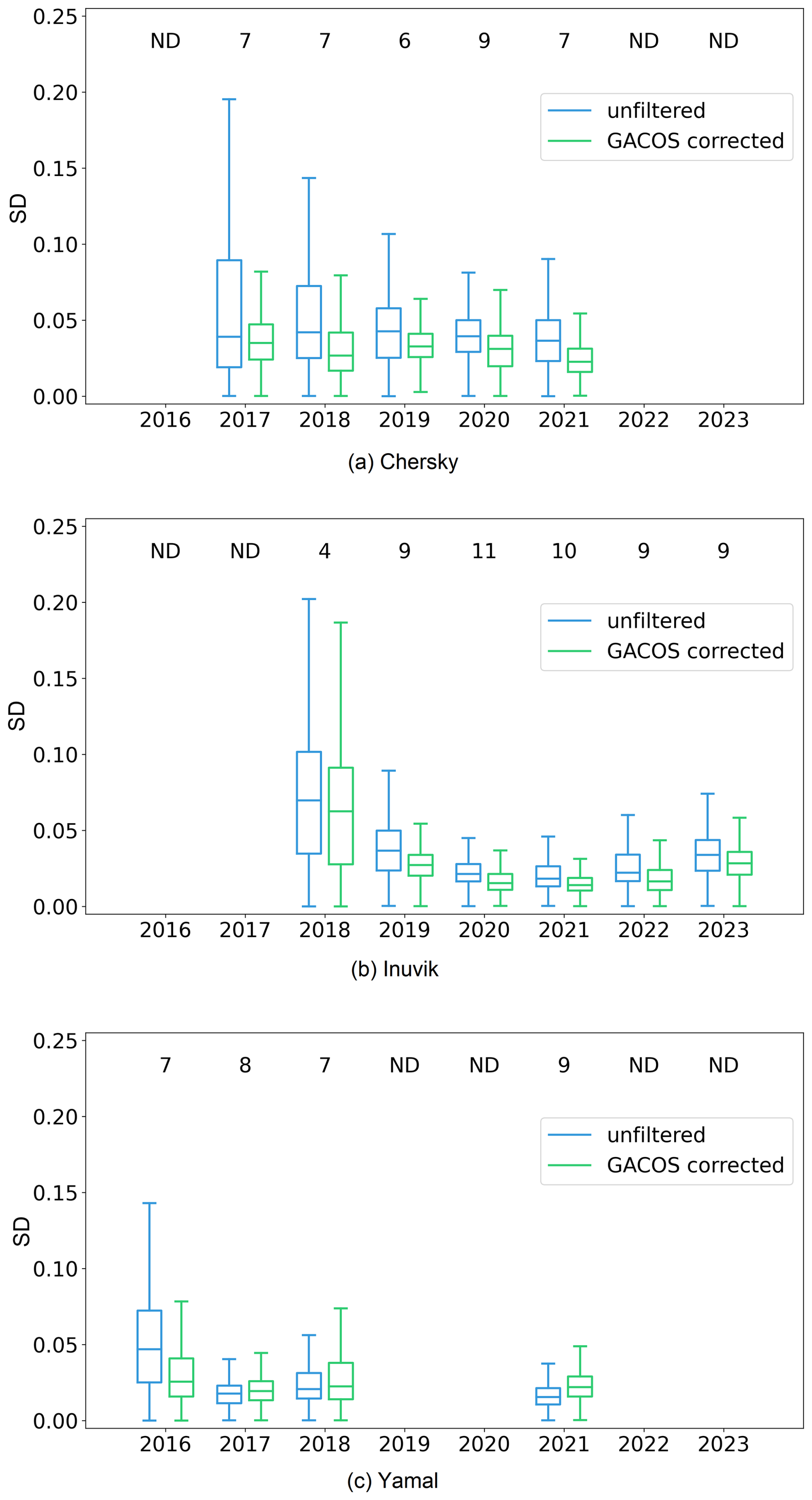
Figure 5Boxplots of standard deviations of the phase residuals for the whole processed scenes (terrain slopes of >5° were masked out) for unfiltered and GACOS-corrected results for (a) Chersky, (b) Inuvik and (c) Yamal. The number of used Sentinel-1 scenes is specified on top of the plots.
5.2 Soil moisture
5.2.1 Soil moisture comparison – Yamal and Inuvik
Comparing the displacement rates to soil moisture measurements (Fig. 6a) showed higher αDDT rates and therefore greater subsidence signal values for points with higher soil moisture for the Yamal study site. As the soil moisture measurements at the Inuvik site were conducted under drought conditions, the soil moisture values tend to be lower. The relationship identified for the Yamal site was confirmed for moisture values below 50 % vol. However, values for higher soil moisture deviated from this trend.
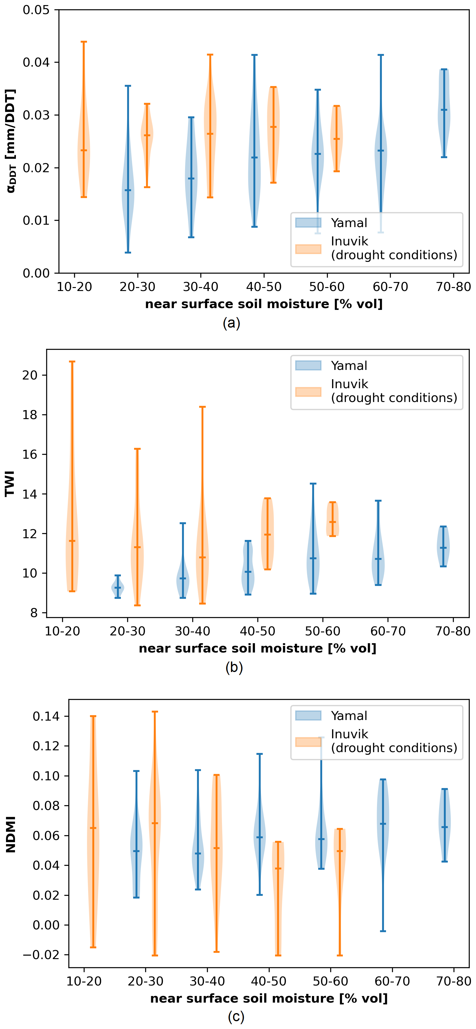
Figure 6Distribution of (a) GACOS-corrected αDDT values, (b) TWI values and (c) NDMI values for near-surface soil moisture bins of Yamal and Inuvik (at minimum six samples per bin).
Similarly, the TWI and NDMI were compared to in situ near-surface soil moisture values. Higher TWI values were associated with higher soil moisture levels in the Yamal region (Fig. 6b). However, the comparison for the Inuvik region did not yield consistently increasing TWI values with rising soil moisture, with deviations found for moisture bins below 30 % vol. The NDMI values exhibited only low spread, and their comparison with near-surface soil moisture data revealed no discernible stringent relationship. While NDMI values tend to be lower for low soil moisture levels in Yamal, the opposite was observed for the Inuvik region.
5.2.2 Accuracy assessment – Yamal
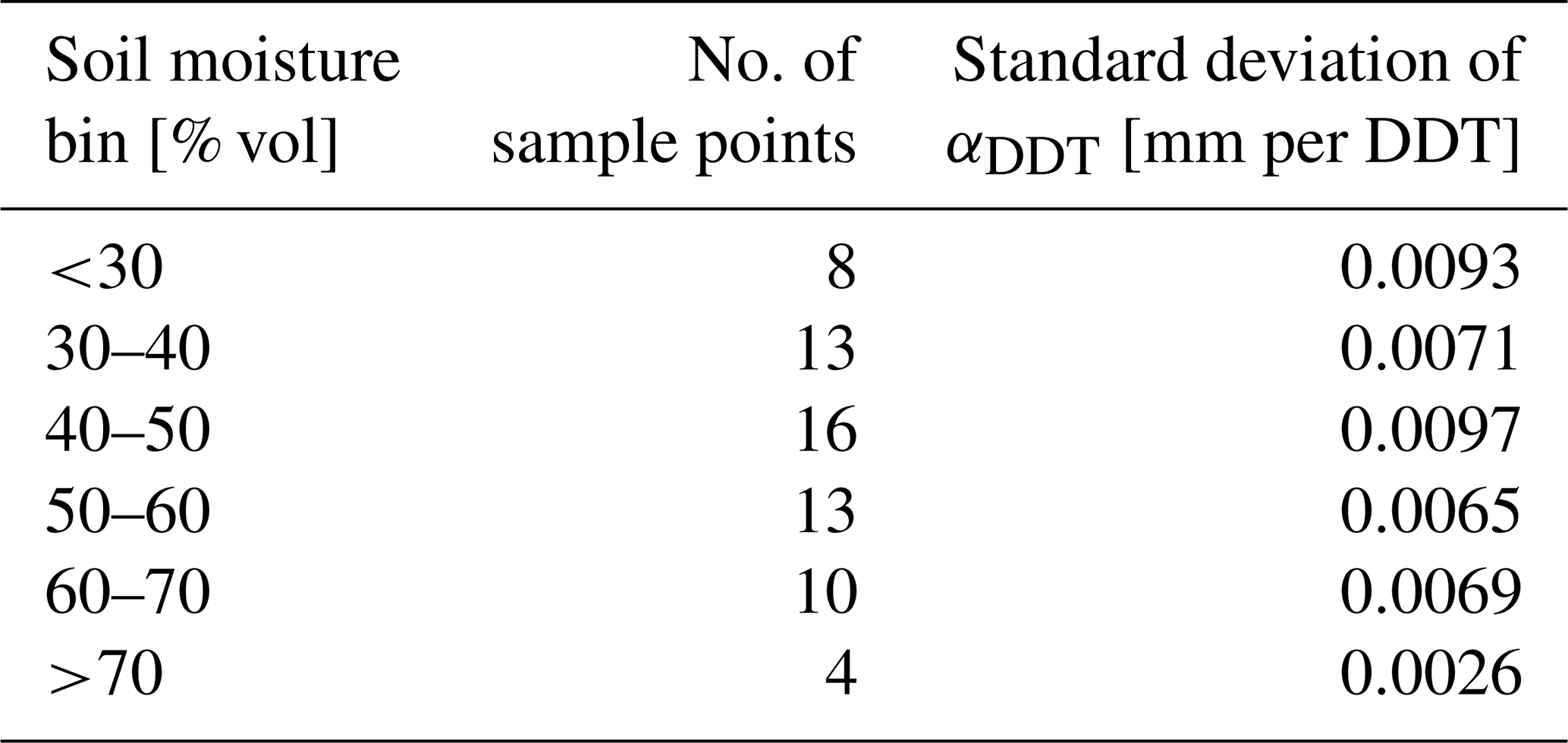
In order to derive a measure of quality for the applicability of αDDT values as a soil moisture proxy, a linear relationship for the Yamal calibration dataset was derived (Fig. 7a). For this, the median αDDT values of six soil moisture bins were calculated. The number of sample points per soil moisture bin ranges from 4 (soil moisture range <70 % vol) to 16 (soil moisture range 40 %–50 % vol). The standard deviations of αDDT for each bin are below 0.0097 [mm per DDT] (Table 4). The obtained linear regression has a coefficient of determination of R2=0.72 for the αDDT values (Fig. 7a) compared to 0.68 of the values (Fig. 7b). While the intercept of the linear regression for αDDT values is statistically insignificant with a P value of 0.91, the slope of the regression has a P value of 0.03, indicating statistical significance. Values of >60 % vol reveal greater deviations from what appears to be a nearly perfect correlation of values of <60 % vol, with P values of 0.0036 and 0.0008 for intercept and slope, respectively.
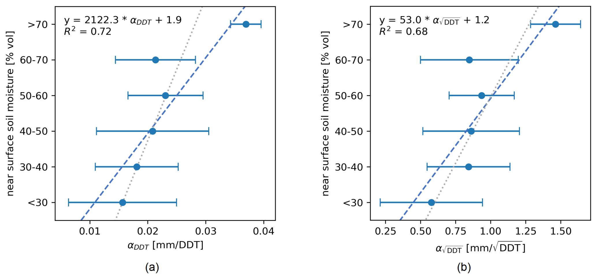
Figure 7Relationship of averaged (10 % vol bins) in situ near-surface soil moisture of the Yamal calibration dataset with (a) median αDDT values and (b) median values for each bin. (αDDT and values represent median values of all years.) Error bars indicate standard deviation per bin. The dashed line depicts the linear regression of all depicted points (equation and R2 indicated on top left). The dotted line shows the relationship of the moisture values of < 60 % vol.
Table 4Count and standard deviation of near-surface soil moisture sample points (Yamal) for each bin value used in Fig. 7a.
Although the linear regression excluding values >60 % appears to show a better fit, it does not follow physical intuition, as its intercept is −37.6 % vol and therefore not applicable for αDDT values closer to 0. The derived equation for all six moisture bins (equation given in Fig. 7a) was subsequently used to predict soil moisture values of the validation dataset (Fig. 8). A RMSE of 14 % vol was delineated for the validation data.
For the purpose of using αDDT as an approximation for soil moisture conditions, we also calculated the accuracy of a possible classification of predicted soil moisture values within the soil moisture bins (indicated in Fig. 7). For these six classes, an accuracy of 25 % is achieved. A reduction of classes into three bins of <40 %, 40 %–60 % and >60 % vol would result in an accuracy of 53 % (maps of categorized soil moisture are presented in Fig. 9).
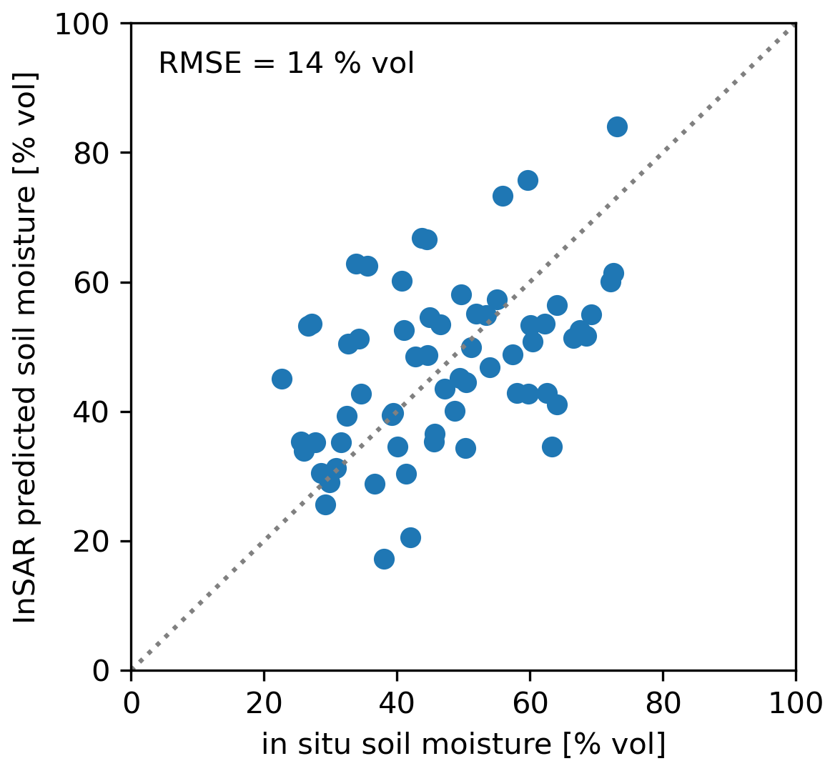
Figure 8Scatterplot of in situ soil moisture values and calculated soil moisture values for the validation dataset of Yamal (used soil-moisture – αDDT relationship; see Fig. 7a). The 1:1 line is depicted as a dotted grey line.
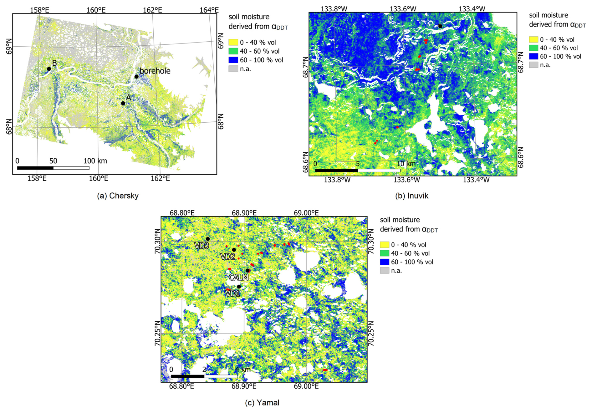
Figure 9Maps of categorized soil moisture derived from InSAR-based αDDT for (a) Chersky, (b) Inuvik and (c) Yamal. All regions are masked for slopes >5°. The Chersky region has additionally been masked for areas higher than 150 m due to temperature lower than 2 °C or more (according to ERA5) than in lower regions during the Sentinel-1 acquisition time. The “n.a.” values represent those that fall outside the valid range. Panels (b) and (c) show subsets of the processed regions, depicting the area where in situ data are available.
To compare this accuracy assessment to other remotely sensed soil moisture products, we investigated values of ESA's CCI soil moisture product (Gruber et al., 2019; Dorigo et al., 2017; Preimesberger et al., 2021). Due to the coarser resolution of 0.25°, our in situ data are covered by only two pixels. The mean soil moisture values for the investigation period are only 19 %–22 % vol for the passive microwave product and 18 % vol for the combined solution (passive and active microwave; see Fig. 10). These products have an RMSE of 30 % vol and 33 % vol for passive and combined solutions, respectively,
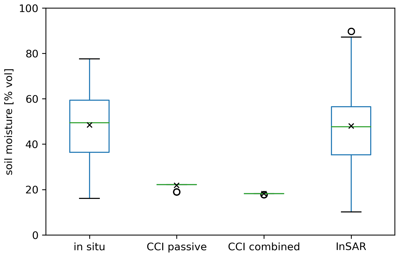
Figure 10Boxplot of in situ measured near-surface soil moisture values compared to values of the CCI soil moisture products (passive and combined product; Gruber et al., 2019; Dorigo et al., 2017; Preimesberger et al., 2021) and soil moisture values calculated with the InSAR approach for Yamal. Black x's represent mean values, and circles indicate outliers.
6.1 Soil moisture
Our InSAR-derived soil moisture approach delivers static values intended to serve as a proxy for general soil moisture conditions. While yearly products are feasible, median values are recommended to account for irregular values caused by uncorrected sources of error.
It is important to note that the relationship between αDDT and soil moisture was derived using in situ measurements of near-surface soil moisture. However, since thaw subsidence observed via InSAR reflects an integrated response from the entire thawed soil column (Liu et al., 2012; Chen et al., 2023), αDDT likely represents a weighted average of soil moisture across the active layer. Given the pronounced vertical variations in soil moisture and ice content in Arctic lowlands, using in situ near-surface soil moisture data may introduce potential uncertainty when interpreting InSAR-derived soil moisture as representative of the entire active layer.
Our investigations showed higher subsidence values for points of higher in situ near-surface soil moisture compared to dryer ones (Fig. 6a). This effect could be demonstrated for both study sites (Yamal and Inuvik). The relationship was more pronounced at the Yamal site, where in situ data measurements were conducted under normal moisture conditions. This observed relationship aligns with findings from Antonova et al. (2018), who identified more prominent subsidence in wetter parts of thermokarst basins. They attributed this to higher ground ice contents of these parts and higher ground heat flux found in wet parts due to their higher thermal conductivity.
Other wetness indices were compared with in situ near-surface soil moisture data, similar to previous αDDT investigations. This analysis aimed to evaluate the performance of αDDT relative to the other indices, specifically to determine whether these indices also demonstrated strong correlations with the in situ measurements. The NDMI derived from multispectral data (Gao, 1996) exhibited varying correlations with soil moisture values across the investigated study sites at in situ sampling point locations (Fig. 6c). The TWI (Beven and Kirkby, 1979), a static wetness index derived from topographic information and often used as a proxy for soil moisture, exhibited similar performance to the InSAR results at the Yamal site (Fig. 6b). However, at the Inuvik site, the analysis did not indicate the suitability of TWI as a measure for soil moisture. These findings suggest a better suitability of αDDT for deriving soil moisture conditions.
To quantify the performance of the investigated method, results were evaluated for their correlation with in situ soil moisture measurements. An empirical function for a calibration dataset was derived and assessed for its accuracy using a validation dataset. The in situ dataset from Yamal was chosen as it was collected under typical moisture conditions rather than drought conditions. Binned and averaged in situ soil moisture and αDDT data yielded a comparably high coefficient of determination of 0.72 (Fig. 7a), slightly higher than the alternative approach based on values (Fig. 7b). It was noted that excluding higher soil moisture levels of >60 % vol would result in nearly perfect correlation for αDDT values. However, to account for all relevant moisture levels, the function derived from all moisture values was further used. This function also appears to be more plausible, as its intercept is 1.9, which would mean no deformation for basically dry soils. However, it should be noted that the coefficient of determination for un-averaged calibration data would be only 0.15. Binning was conducted (comparable to Bartsch et al., 2020) to account for differences in the in situ data's representativeness (point measurements versus spatial resolution of InSAR data). A comparison of in situ observed moisture levels to predicted ones for the validation dataset revealed no larger discrepancies for higher soil moisture values (Fig. 8). A RMSE of 14 % vol could be achieved.
Results were further compared to the CCI soil moisture product. A direct comparison between the CCI soil moisture dataset and the InSAR data is challenging due to the significant difference in their spatial resolutions. The CCI dataset has a much coarser resolution, with each pixel covering an area approximately 106 times larger than that covered by each pixel in the InSAR dataset. Consequently, any differences observed between the two datasets when comparing them to in situ data may be partly attributed to this resolution discrepancy. The CCI soil moisture comparison showed RMSE values that are twice the value of the InSAR approach. The moisture values of the CCI products are much lower than was measured in the field (Fig. 10), with just 1 % of field data being lower than what was indicated by the CCI soil moisture products (passive and passive–active combined). The active product of CCI soil moisture was not used, as it provides only saturation values. However, comparisons of in situ values and the active product derived from ASCAT were previously performed by Högström et al. (2018) for five Arctic regions. The in situ data were scaled to the satellite product to enable comparison. ASCAT has been shown to be drier than in situ data in most cases, which agrees with our result.
We further assessed the accuracy of a potential soil moisture classification product based on αDDT values. A classification with six moisture classes would yield a 25 % accuracy. Therefore, it is suggested to only use three moisture categories, for which the accuracy would improve to 53 %. It should be noted that assessed soil moisture values used for the derivation of the linear relationship were within the range of 20 %–80 % vol. However, it can be assumed that a proposed classification of three moisture categories is conservative enough to also account for moisture values outside of the tested range.
6.2 DDT normalization
As shown in Fig. A2, the time series of GACOS-corrected results still show interfering fluctuations. However, this issue may be addressed by simply utilizing the slope of the time series (αDDT). What is further visible (Fig. A2) is the data gap at the beginning of the time series, which may differ in length for different years or study regions. Nevertheless, this should be of lesser concern if a linear trend is to be assumed over DDT, which, based on our findings, appears to be mostly the case in our study regions. It is important to note, however, that active layer thaw is presumed to be greater in early summer and decreasing in August and September (Short et al., 2014). Although this is not consistently reflected in our DDT plots (Fig. A2), it cannot be completely ruled out.
The uncertainties for ERA5 data in the Arctic, which were used to derive DDT, represent another potential source of error. A comparison of ERA5 values with those from an ERA5-independent automatic weather station near Chersky revealed slightly lower measured values at the weather station than ERA5 values (see also Fig. 13). The seasonal maxima of DDT for the years 2016–2022 (missing data for 2018) differed by about 100–150 °C, which corresponds to approximately 7 %–10 % of the maximal ERA5 DDT values and would result in slightly different αDDT values. DDTs of the automatic weather station yielded αDDT values 17 % lower than those of ERA5 (Fig. 13).
It also needs to be considered that ERA5 air temperatures at 2 m height may deviate from topsoil temperatures, resulting in variations in αDDT values. In order to investigate these variations, we compared ERA5 results to ground temperatures at four points in Yamal, measured between October 2016 and August 2017 near the surface using iButton devices (Fig. 2). While the point at the CALM grid showed good agreement with ERA5 values in the positive temperature range, the other points demonstrated lower in situ temperatures than ERA5 temperatures (Fig. 11). Although the in situ time series ended on 24 August and maximum DDT values were not yet reached (80 % of maximal ERA5 DDT value), we compared maxima of ERA5 and in situ DDT values for this date (aggregated from values shown in Fig. 11). Only the in situ values of the CALM grid had higher DDT values than ERA5 (147.2 °C higher, 21 % of ERA5). The other points showed higher differences, ranging from 340 to 404 °C, which is 48 % to 55 % of the maximal ERA5 value on 24 August. These differences can be explained by insulating vegetation cover, as ERA5 represents air temperature at 2 m compared to near-surface soil temperature. Furthermore, quality issues and the coarse resolution of ERA5 data may play a role. The αDDT values differ significantly from ERA5-derived αDDT values in the range of −0.087 to 0.007 [mm per DDT] (Fig. 12).
αDDT derived with DDT values of even deeper soil layers would naturally deviate even more from those derived with ERA5 data (Figs. 12 and 13). The resulting displacement rates (αDDT) are shown to be larger for deeper soil layers, as derived from borehole data of 50 cm depth (Yamal) and 4 and 8 cm depths (Chersky).
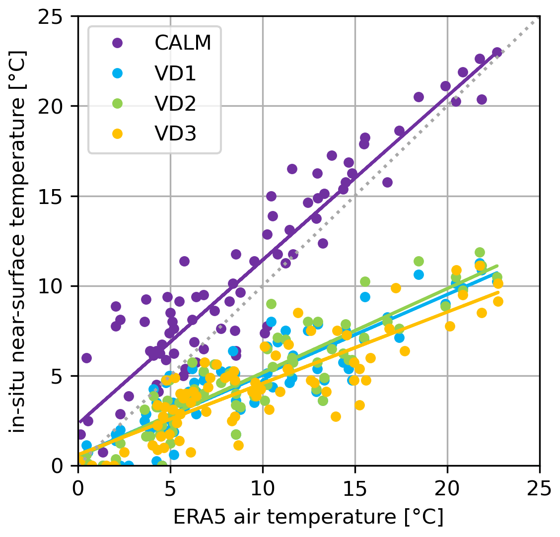
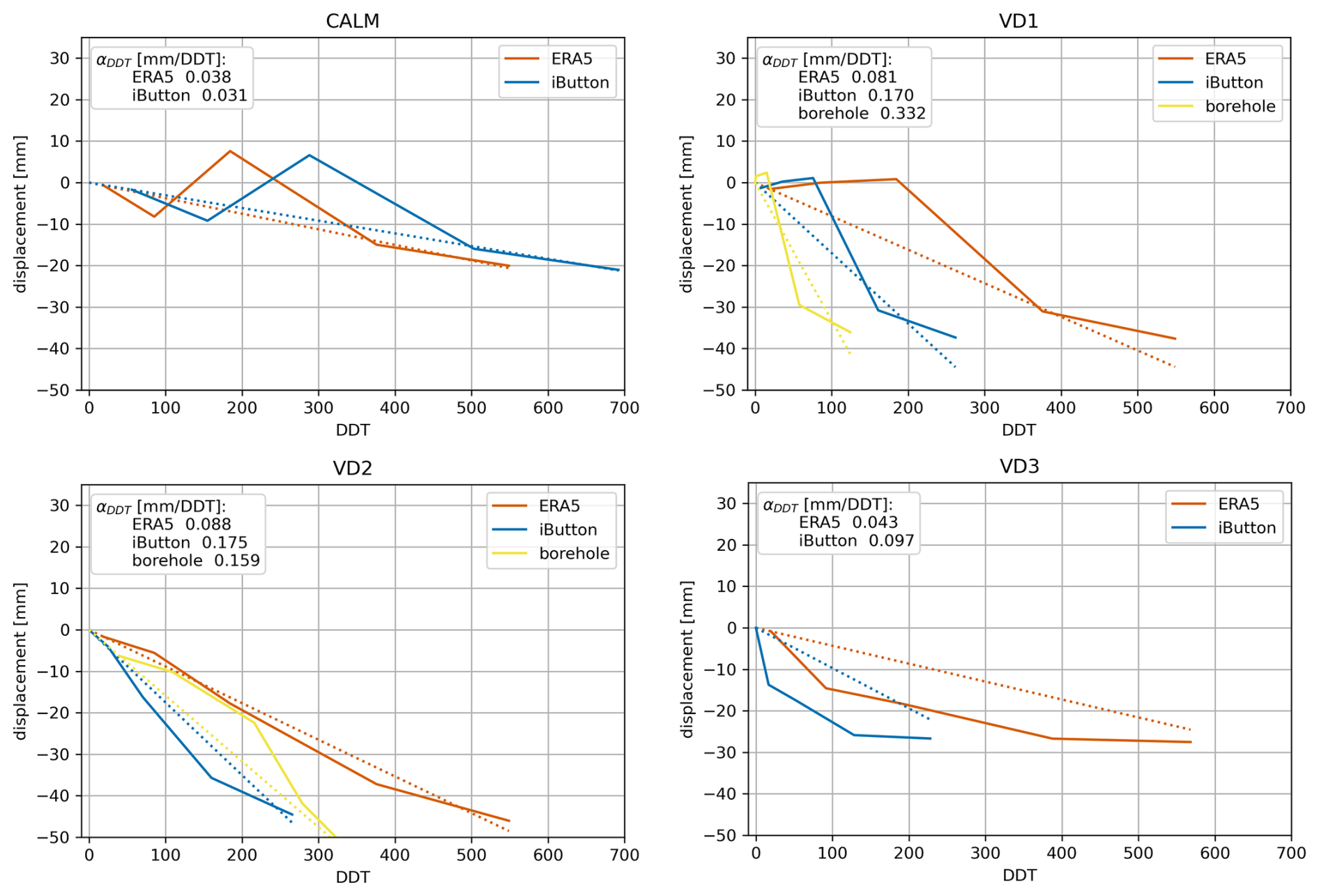
Figure 12InSAR displacements of the thawing season 2017 by degree day of thaw (DDT) for four sample points in Yamal. DDT was derived from ERA5 air temperature at 2 m height, in situ near-surface iButton data and borehole temperatures at 50 cm depth (time series shortened due to in situ data availability; see Table 2). Interpolations (linear regression) are plotted as dotted lines. For in situ point locations, see Fig. 2.
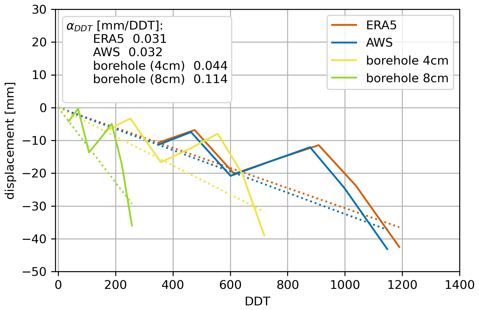
Figure 13InSAR displacements of the thawing season 2017 by degree day of thaw (DDT) for a sample point of the Chersky region. DDT was derived from ERA5 air temperature at 2 m height, automatic weather station (AWS) data, and borehole temperatures at 4 and 8 cm depths. For in situ point location, see Fig. 2.
6.3 Atmospheric corrections
In order to achieve reliable InSAR results for soil moisture comparisons, the issue of atmospheric disturbances had to be addressed. Investigations of displacement time series (Figs. A2, A3 and A4) revealed that the applied spatial filter not only reduces spatial variations but also flattens temporal fluctuations. While a reduction in temporal variations seems to be more reasonable than the often high variability of unfiltered or GACOS-corrected results, the spatially filtered results mostly lacked any large-scale spatial deformations, which may not always represent actual conditions. In this regard, a filter size of 6 km is too small; however, larger filter sizes would not account for small-scale effects of the turbulent atmosphere. Comparisons with in situ subsidence values (Fig. 4) further illustrated that spatially filtered results were greatly reduced in magnitude. This not only led to lower subsidence values but also resulted in measured heave signals, which deviate from in situ measured results. While additional temporal filtering is recognized as an important aspect of InSAR time series analysis, it was not tested in this study, as αDDT, representing the linear regression rate, is unlikely to be significantly influenced by further temporal filtering.
GACOS-corrected products, on the other hand, showed promising results. After correcting GACOS data for encountered artefacts (see Fig. S1 in the Supplement), the derived results were able to compensate for some improbable summer heave signals visible in the Chersky time series of unfiltered results (Fig. A2). However, some atmospheric effects remained (Fig. A1), which may lead to the encountered fluctuations within the time series. It should also be noted that GACOS can sometimes introduce new artefacts (see also year 2019 of Fig. A4) and may not necessarily guarantee an improvement of results due to scarcity of GPS stations and the coarse weather model resolution. However, the comparison of standard deviations of phase residuals showed improvements compared to unfiltered results, especially for the Chersky and the Inuvik region. As the differences of the median values (unfiltered minus GACOS, Fig. A7) seem to show a dependency on study area, this may indicate varying effectiveness of GACOS corrections depending on region. The differing results for the Yamal region, however, also indicate that, although in this area the GACOS corrections may not always lead to an improvement (see also Fig. A3), some years may still benefit from this correction. One reason for the performance differences observed in various regions may be the coarse temporal resolution of the weather model used in GACOS for the turbulent component. Although corrections are provided for the specific times of satellite acquisitions, the interpolated solution may align more closely with the 6 h intervals of the weather model in some areas than in others. Moreover, the limited availability of GPS stations in certain regions may also contribute to these variations.
Even though the standard deviation values of the phase residual were mostly slightly higher for GACOS-corrected results than for unfiltered ones in the Yamal region, the comparison to in situ subsidence data showed the closest match for GACOS within this area.
The overall lower InSAR subsidence compared to in situ values (Fig. 4) has also been reported in other studies in Arctic regions (Short et al., 2014; Antonova et al., 2018) and may have multiple causes. First, in situ measurements are point measurements, and medium-scale InSAR measurements may therefore underestimate true displacements due to spatial averaging (Short and Fraser, 2023). Furthermore, it cannot be excluded that the selected reference point (airstrip at Bovanenkovo) also experiences some degree of surface deformation. The assumption of a linear relationship between DDT and thaw subsidence may also play a role. Potential faster subsidence rates during the unmonitored beginning of the thawing season may lead to an underestimation of subsidence values. In addition, soil moisture variations may have an effect on measured InSAR results. Soil drying, which leads to a line-of-sight shortening, results in an uplift signal (Zwieback et al., 2015), potentially contributing to lower subsidence values compared to in situ measurements. The effect is estimated to be 10 %–20 % of the radar wavelength (Zwieback et al., 2017). Further effects were reported due to vegetation growth and the inherent decrease in plant moisture (Zwieback and Hajnsek, 2016), which may also cause additional uplift signals. An investigation of soil moisture change at Trail Valley Creek (data source of soil moisture time series: Boike et al., 2023) for consecutive Sentinel-1 acquisitions, compared with changes in InSAR displacement signals (see Fig. 14), revealed no significant relationship, leading to the assumption that this source of error is of subordinate importance in this case. Furthermore, it should be noted that validating InSAR displacement values was not the primary objective of this study. An underestimation of subsidence values is less relevant if it occurs consistently, as the linear relationship between displacement and moisture values was derived from these biased data.
6.4 Limitations for InSAR processing
The demonstrated relationship between soil moisture and InSAR subsidence signals exemplifies the potential of InSAR data to derive maps of soil moisture classes needed for upscaling carbon fluxes and climate modelling. However, some inhibiting factors have to be addressed. As illustrated, GACOS corrections are an adequate and easily implementable solution to reduce atmospheric effects. Some remnants may persist, especially effects of the turbulent atmosphere (Li et al., 2022). Furthermore, ionospheric effects are not accounted for with this correction. It is therefore essential to carefully select interferograms and use thawing seasons of years with minimal interfering effects in the derivation of soil moisture class maps.
Additionally, the selection of an adequate reference point is crucial and can prove to be difficult. Moreover, errors may increase with distance from the reference point (Short, 2017; Antonova et al., 2018), which has to be taken into account when processing whole Sentinel-1 scenes.
Another potential source of uncertainty is the impact of time-varying soil moisture on interferometric phase. A link between subsidence change and soil moisture change could not be observed at the study site of Trail Valley Creek (Fig. 14). The variation in soil moisture between consecutive acquisition dates is mostly below 10 % vol, which is much lower compared to other studies (Wig et al., 2023). Therefore, the influence of soil moisture change appears subordinate compared to other disturbances (including atmosphere). However, this phase term remains coupled with the ground motion information and thus persists as a potential source of error in the results.
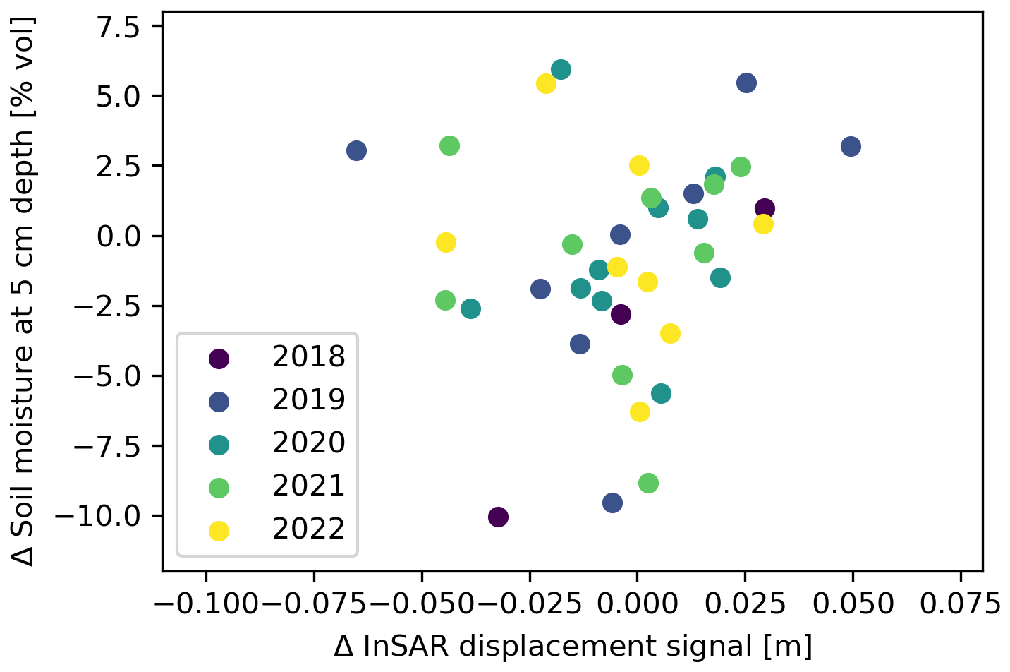
Figure 14Comparison of InSAR displacement signals from consecutive Sentinel-1 acquisition dates and corresponding soil moisture change (derived from Boike et al., 2023), measured at Trail Valley Creek in the Inuvik study area.
6.5 Permafrost features characterization
Delineated soil wetness should also be reflected in certain land-cover features related to polygonal tundra. Slightly higher αDDT and subsidence can indeed be observed for areas with polygonal features compared to other non-wetland tundra (Figs. A5 and A6). However, no visible differentiation is detectable between high-centred and low-centred polygons. The derived αDDT values for the subsidence of the polygonal features are similar to those of wetlands without visible polygonal features. Both areas with low- and high-centred polygons are expected to be characterized by strong microtopography, resulting in a mix of wet and dry parts, which leads to medium αDDT values (not as low as for in situ points with very high soil moisture contents; see Fig. 6a).
A representation of soil moisture classes is in high demand for applications in Arctic permafrost regions. In this study, we proposed a novel approach for deriving a soil moisture index based on InSAR subsidence signal rates. We illustrated the relationship between Sentinel-1 InSAR subsidence signal per DDT and surface soil moisture, with lower rates attributed to surface subsidence signals for drier regions and seasons, demonstrating its potential as a proxy for soil moisture classes. Compared to conventional coarser-scale datasets such as ESA's CCI soil moisture product, which underestimated in situ values with an RMSE of around 30 % vol, our proposed method achieved an RMSE of 14 % vol. Although this approach provides only static information and does not account for seasonal fluctuations in soil moisture, it is assumed to be a valid indicator for general or predominant moisture conditions for permafrost regions. It is recommended to distinguish only three soil moisture categories. Its application for upscaling carbon fluxes and climate modelling remains to be tested.
Spatial patterns of wet and dry areas can be derived, but not all features typical for permafrost can be resolved. It is also pointed out that the ERA5 air temperature at 2 m height used for the calculation of DDTs may result in different subsidence rates (αDDT) compared to using topsoil temperatures.
Phase delays arising from soil moisture changes represent a limitation that should be considered in future studies, with potential benefits from leveraging insights gained from ongoing research.
Limiting factors for the utilization of InSAR also include atmospheric effects. Atmospheric correction is therefore essential for InSAR applications to derive reliable results, especially in cases where coherence loss prevents the use of interferograms overlapping in time. We tested two easy-to-apply filtering methods for implementation in Arctic regions. Our study showed that while spatial filtering corrects for spatial and temporal variabilities, the suppression of larger-scale displacement signals leads to a reduction of subsidence signal values, resulting in a poorer match with in situ values. GACOS-corrected results showed a reduction of atmospheric effects within the investigated time series, as well as an improvement in standard deviation values of phase residuals, and often the best match with in situ subsidence values. However, it should be noted that smaller-scale tropospheric variations (<75 km) may not be corrected (Murray et al., 2019). While long-wavelength components may be accounted for, the turbulent atmosphere phase mostly cannot be removed (Li et al., 2022). Nevertheless, our investigations showed that GACOS-corrected results are more suitable than spatial filtering and better suited for the derivation of soil moisture classes.
In upcoming years, InSAR processing of Sentinel-1 data are anticipated to benefit from the release of the extended timing annotation dataset (ETAD), which includes correction layers for tropospheric delay and ionospheric delay, among others (Gisinger et al., 2022). Similar to GACOS, the tropospheric delay is based on weather model data. However, data provision is currently only planned for newly acquired scenes, which prohibits its application for past years.
L-band missions, which have the potential to better preserve coherence, would reduce the importance of the investigated correction methods. Comprehensive L-band datasets are, however, mostly acquired on demand, and available data acquisition dates rarely meet requirements for the proposed investigation method. Nevertheless, with the launch of the upcoming NISAR (NASA-ISRO Synthetic Aperture Radar) mission, improved data coverage is anticipated in the near future.
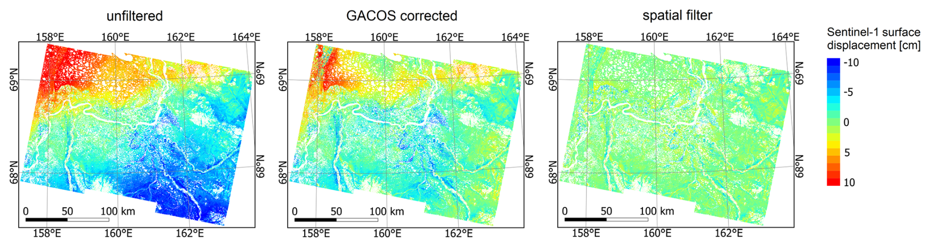
Figure A1Comparison of unfiltered, GACOS-corrected and spatial filter InSAR results for the Chersky study region for 23 June 2017–3 September 2017.
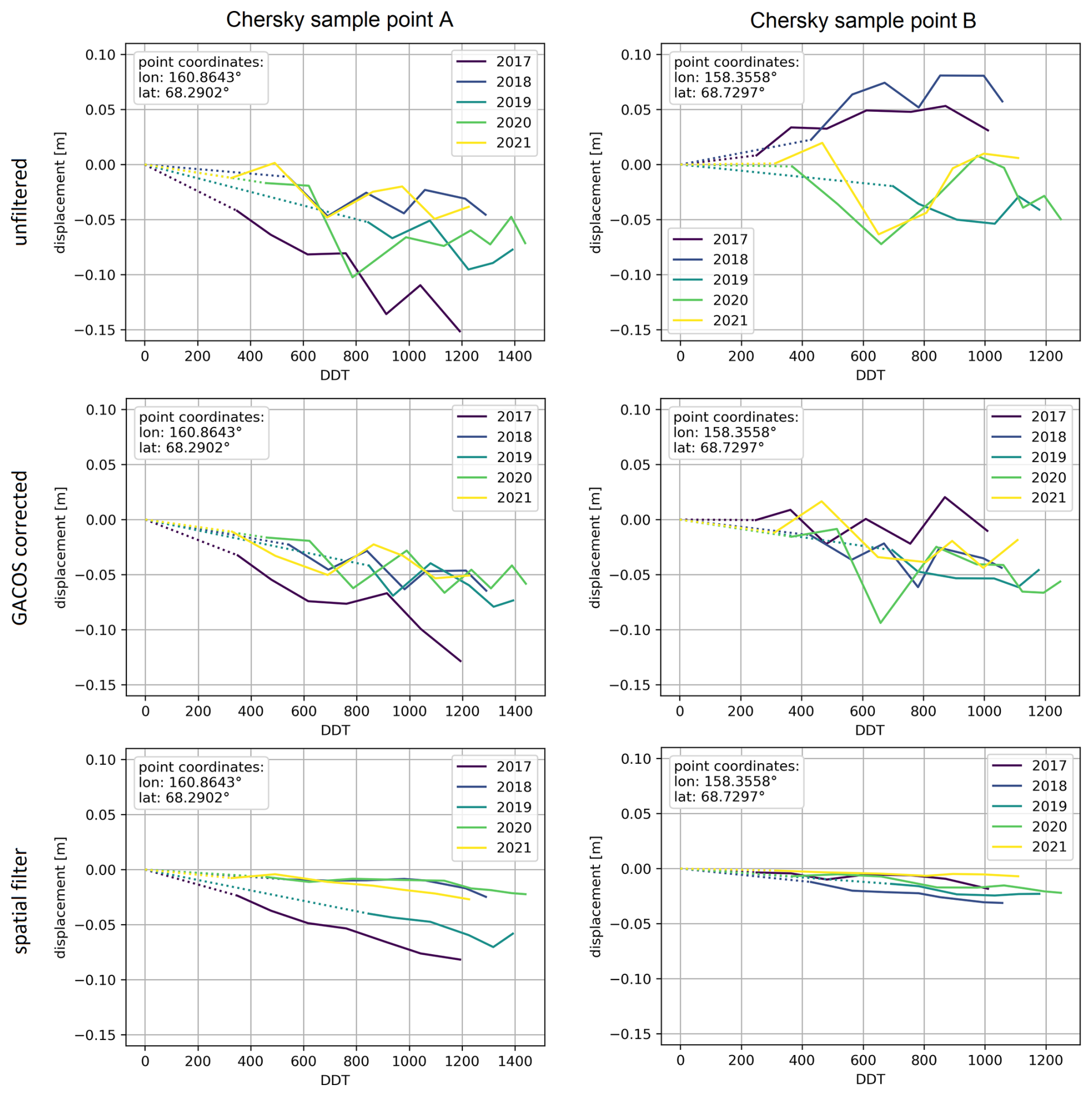
Figure A2Sample point displacements by degree day of thaw (DDT) for Chersky, accounting for the early thaw data gap in InSAR time series by extrapolation (approach following Bartsch et al., 2019; dotted lines correspond to the linearly extrapolated part of the time series). For point locations, see Fig. 2.
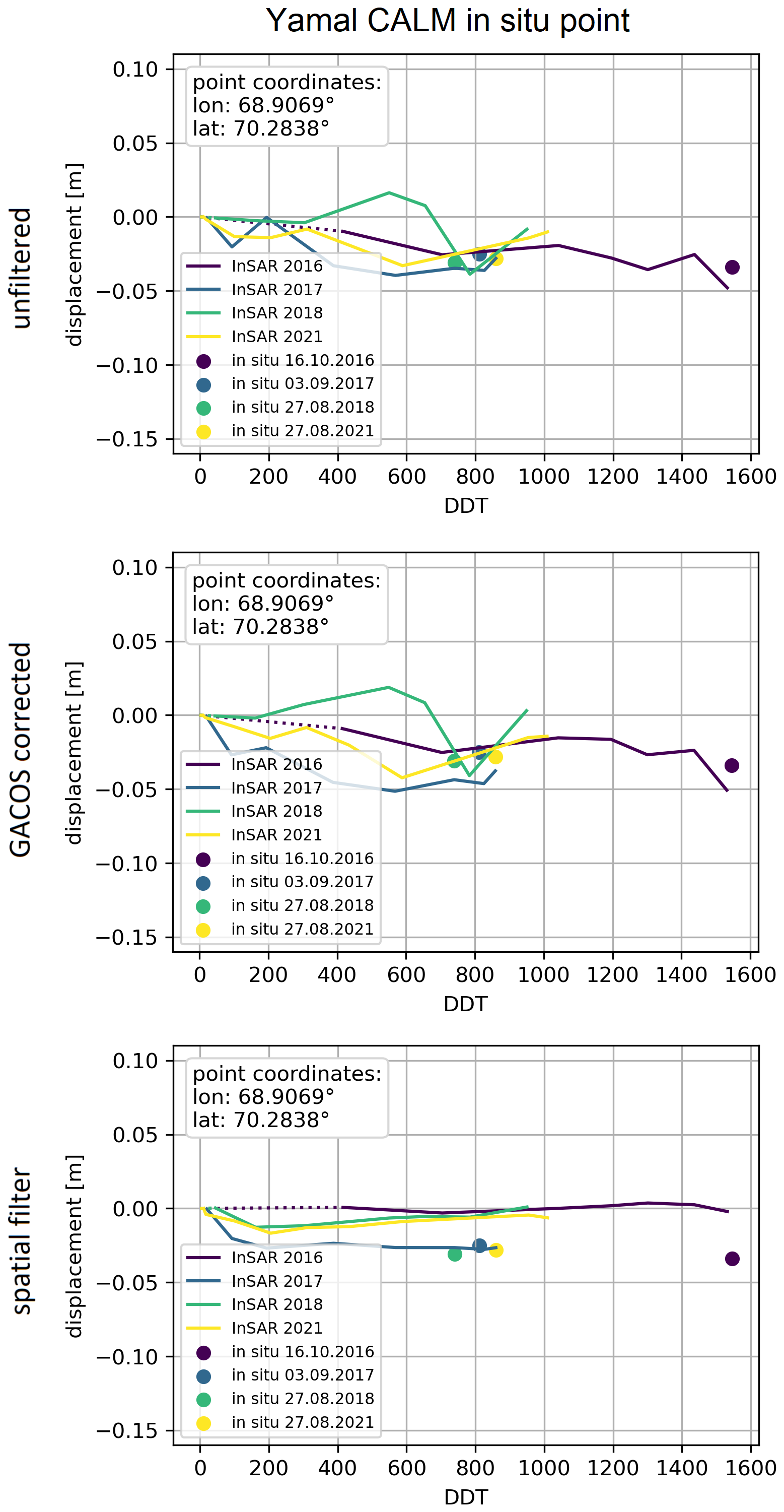
Figure A3Displacements by degree day of thaw (DDT) of a sample point location with in situ subsidence measurements on the CALM grid in Yamal. The early thaw data gap in the InSAR time series was accounted for by extrapolation (approach following Bartsch et al., 2019; dotted lines correspond to the linearly extrapolated part of the time series). For CALM grid locations, see Fig. 2.
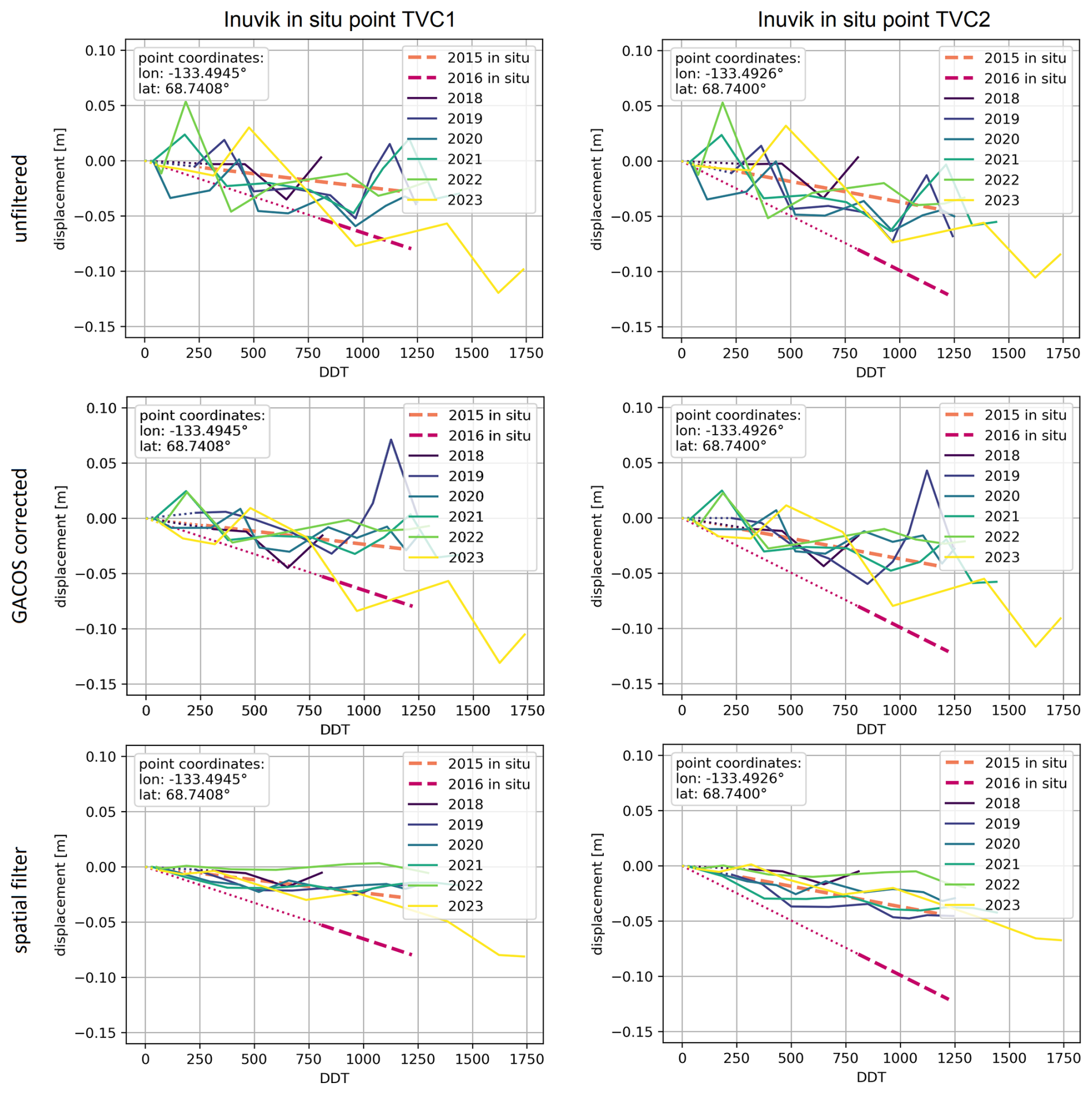
Figure A4Displacements by degree day of thaw (DDT) of two sample points with in situ subsidence measurements for the years 2015 and 2016 near the Trail Valley Creek (TVC) research station (Inuvik region). The early thaw data gap in the InSAR time series was accounted for by extrapolation (approach following Bartsch et al., 2019; dotted lines correspond to the linearly extrapolated part of the time series). For TVC location, see Fig. 2.
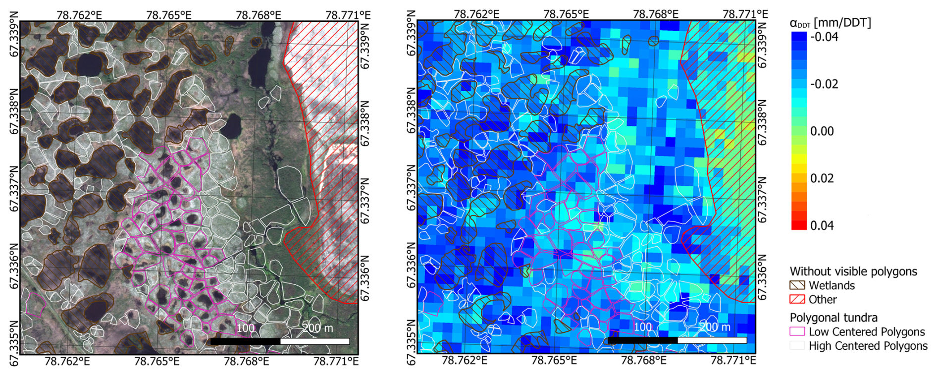
Figure A5Subset of digitized land-cover features: left with WorldView-3 image as background map and right with αDDT.
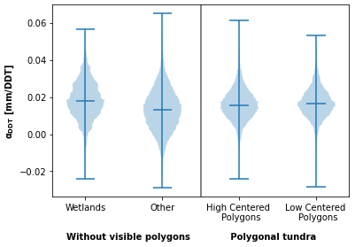
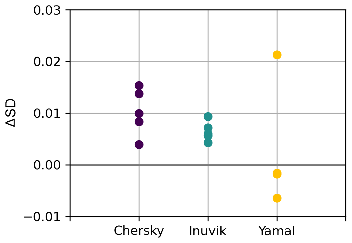
InSAR data were processed using the GAMMA software. All further processing was performed using freely available software (e.g., GDAL, Rasterio, QGIS).
Sentinel-1 satellite data are freely available from the Copernicus Data Space Ecosystem (https://dataspace.copernicus.eu, Copernicus Data Space Ecosystem, 2023). GACOS products are provided by Newcastle University and are freely accessible to users at http://www.gacos.net (Yu and Li, 2024). Auxiliary data (ERA5, Copernicus DEM, ArcticDEM, Landsat 8 and ESA’s CCI soil moisture product) are openly available, and data access information is provided in the reference list. In cases where the in situ data used are freely accessible, they are referenced accordingly and listed in the reference list.
The supplement related to this article is available online at https://doi.org/10.5194/tc-19-1103-2025-supplement.
BW and AB developed the concept for the study. BW analysed the results and wrote the first draft of the manuscript. TS and NJ provided expertise on InSAR processing. AK, EB, ML, RK, HS, CB, XM and MG contributed to the in situ surveys and evaluation data processing. AB, TS, ML, RK and MG contributed to the writing of the manuscript.
The contact author has declared that none of the authors has any competing interests.
Publisher’s note: Copernicus Publications remains neutral with regard to jurisdictional claims made in the text, published maps, institutional affiliations, or any other geographical representation in this paper. While Copernicus Publications makes every effort to include appropriate place names, the final responsibility lies with the authors.
We would like to thank Christophe Magnard of GAMMA Remote Sensing for providing the implementation of the GACOS correction within the Gamma software, Veronika Doepper from the Helmholtz Einstein International Berlin Research School in Data Science (HEIBRIDS), and Birgit Heim from the Alfred Wegener Institute for Polar and Marine Research for field work support in the framework of the AWI CA-Land_NWCanada2023 expedition.
This research has been supported by the European Research Council H2020 (project no. 951288, Q-Arctic), the European Space Agency (project CCI+ Permafrost 4000123681/18/I-NB) and the Ministry of Science and Higher Education of the Russian Federation (grant no. FWRZ-2021-0012). Publisher's note: the article processing charges for this publication were not paid by a Russian or Belarusian institution.
This paper was edited by Regula Frauenfelder and reviewed by Lin Liu and one anonymous referee.
Anders, K., Antonova, S., Beck, I., Boike, J., Höfle, B., Langer, M., Marsh, P., and Marx, S.: Multisensor ground-based measurements of the permafrost thaw subsidence in the Trail Valley Creek, NWT, Canada, 2015–2016, PANGAEA [data set], https://doi.org/10.1594/PANGAEA.888566, 2018. a, b
Antonova, S., Sudhaus, H., Strozzi, T., Zwieback, S., Kääb, A., Heim, B., Langer, M., Bornemann, N., and Boike, J.: Thaw Subsidence of a Yedoma Landscape in Northern Siberia, Measured In Situ and Estimated from TerraSAR-X Interferometry, Remote Sens., 10, 494, https://doi.org/10.3390/rs10040494, 2018. a, b, c
Babkin, E. M., Khomutov, A. V., Dvornikov, Y. A., Khairullin, R. R., and Babkina, E. A.: Relief changes of the peat plateu with melting of polygonal-wedge ice in the northern part of the Pur-Taz interfluve, Regional Environmental Issues, 4, 115–119, https://doi.org/10.24411/1728-323X-2018-14115, 2018. a, b
Barrett, B. W., Dwyer, E., and Whelan, P.: Soil Moisture Retrieval from Active Spaceborne Microwave Observations: An Evaluation of Current Techniques, Remote Sens., 1, 210–242, https://doi.org/10.3390/rs1030210, 2009. a
Bartalis, Z., Wagner, W., Naeimi, V., Hasenauer, S., Scipal, K., Bonekamp, H., Figa, J., and Anderson, C.: Initial soil moisture retrievals from the METOP-A Advanced Scatterometer (ASCAT), Geophys. Res. Lett., 34, L20401, https://doi.org/10.1029/2007GL031088, 2007. a
Bartholomé, E. and Belward, A. S.: GLC2000: a new approach to global land cover mapping from Earth observation data, Int. J. Remote Sens., 26, 1959–1977, https://doi.org/10.1080/01431160412331291297, 2005. a
Bartsch, A., Leibman, M., Strozzi, T., Khomutov, A., Widhalm, B., Babkina, E., Mullanurov, D., Ermokhina, K., Kroisleitner, C., and Bergstedt, H.: Seasonal Progression of Ground Displacement Identified with Satellite Radar Interferometry and the Impact of Unusually Warm Conditions on Permafrost at the Yamal Peninsula in 2016, Remote Sens., 11, 1865, https://doi.org/10.3390/rs11161865, 2019. a, b, c, d, e, f, g, h, i, j
Bartsch, A., Widhalm, B., Leibman, M., Ermokhina, K., Kumpula, T., Skarin, A., Wilcox, E. J., Jones, B. M., Frost, G. V., Höfler, A., and Pointner, G.: Feasibility of tundra vegetation height retrieval from Sentinel-1 and Sentinel-2 data, Remote Sens. Environ., 237, 111515, https://doi.org/10.1016/j.rse.2019.111515, 2020. a, b
Bartsch, A., Strozzi, T., and Nitze, I.: Permafrost Monitoring from Space, Surv. Geophys., 44, 1579–1613, https://doi.org/10.1007/s10712-023-09770-3, 2023. a, b, c, d, e
Berardino, P., Fornaro, G., Lanari, R., and Sansosti, E.: A new algorithm for surface deformation monitoring based on small baseline differential SAR interferograms, IEEE T. Geosci. Remote Sens., 40, 2375–2383, https://doi.org/10.1109/TGRS.2002.803792, 2002. a
Beven, K. J. and Kirkby, M. J.: A physically based, variable contributing area model of basin hydrology, Hydrol. Sci. B., 24, 43–69, https://doi.org/10.1080/02626667909491834, 1979. a
Boike, J., Miesner, F., Bornemann, N., Cable, W. L., and Grünberg, I.: Trail Valley Creek, NWT, Canada Soil Moisture and Temperature 2016 et seq, PANGAEA [data set], https://doi.org/10.1594/PANGAEA.962726, 2023. a, b, c, d
Campbell, G. S. and Norman, J. M.: An Introduction to Environmental Biophysics, Springer, New York, 2 edn., https://link.springer.com/book/10.1007/978-1-4612-1626-1 (last access: 4 March 2025), 1998. a, b
Cheţan, M.-A., Dornik, A., Ardelean, F., Georgievski, G., Hagemann, S., Romanovsky, V. E., Onaca, A., and Drozdov, D. S.: 35 Years of Vegetation and Lake Dynamics in the Pechora Catchment, Russian European Arctic, Remote Sens, 12, 1863, https://doi.org/10.3390/rs12111863, 2020. a
Chen, J., Wu, Y., O'Connor, M., Cardenas, M. B., Schaefer, K., Michaelides, R., and Kling, G.: Active layer freeze-thaw and water storage dynamics in permafrost environments inferred from InSAR, Remote Sens. Environ., 248, 112007, https://doi.org/10.1016/j.rse.2020.112007, 2020. a
Chen, R. H., Michaelides, R. J., Zhao, Y., Huang, L., Wig, E., Sullivan, T. D., Parsekian, A. D., Zebker, H. A., Moghaddam, M., and Schaefer, K. M.: Permafrost Dynamics Observatory (PDO): 2. Joint Retrieval of Permafrost Active Layer Thickness and Soil Moisture From L-Band InSAR and P-Band PolSAR, Earth and Space Science, 10, e2022EA002453, https://doi.org/10.1029/2022EA002453, e2022EA002453 2022EA002453, 2023. a, b, c
Colliander, A., Jackson, T. J., Bindlish, R., Chan, S., Das, N., Kim, S. B., Cosh, M. H., Dunbar, R. S., Dang, L., Pashaian, L., Asanuma, J., Aida, K., Berg, A., Rowlandson, T., Bosch, D., Caldwell, T., Caylor, K., Goodrich, D., al Jassar, H., Lopez-Baeza, E., Martínez-Fernández, J., González-Zamora, A., Livingston, S., McNairn, H., Pacheco, A., Moghaddam, M., Montzka, C., Notarnicola, C., Niedrist, G., Pellarin, T., Prueger, J., Pulliainen, J., Rautiainen, K., Ramos, J., Seyfried, M., Starks, P., Su, Z., Zeng, Y., van der Velde, R., Thibeault, M., Dorigo, W., Vreugdenhil, M., Walker, J., Wu, X., Monerris, A., O'Neill, P., Entekhabi, D., Njoku, E., and Yueh, S.: Validation of SMAP surface soil moisture products with core validation sites, Remote Sens. Environ., 191, 215–231, https://doi.org/10.1016/j.rse.2017.01.021, 2017. a
Copernicus Data Space Ecosystem, European Space Agency: Sentinel-1 satellite data, [data set], https://dataspace.copernicus.eu (last access: 4 March 2025), 2023. a
Costantini, M.: A novel phase unwrapping method based on network programming, IEEE T. Geosci. Remote Sens., 36, 813–821, https://doi.org/10.1109/36.673674, 1998. a
Das, K. and Paul, P. K.: Present status of soil moisture estimation by microwave remote sensing, Cogent Geoscience, 1, 1084669, https://doi.org/10.1080/23312041.2015.1084669, 2015. a
De Zan, F. and Gomba, G.: Vegetation and soil moisture inversion from SAR closure phases: First experiments and results, Remote Sens. Environ., 217, 562–572, https://doi.org/10.1016/j.rse.2018.08.034, 2018. a
De Zan, F., Parizzi, A., Prats-Iraola, P., and López-Dekker, P.: A SAR Interferometric Model for Soil Moisture, IEEE T. Geosci. Remote Sens., 52, 418–425, https://doi.org/10.1109/TGRS.2013.2241069, 2014. a
Dini, B., Daout, S., Manconi, A., and Loew, S.: Classification of slope processes based on multitemporal DInSAR analyses in the Himalaya of NW Bhutan, Remote Sens. Environ., 233, 111408, https://doi.org/10.1016/j.rse.2019.111408, 2019. a
Dorigo, W., Wagner, W., Albergel, C., Albrecht, F., Balsamo, G., Brocca, L., Chung, D., Ertl, M., Forkel, M., Gruber, A., Haas, E., Hamer, P. D., Hirschi, M., Ikonen, J., de Jeu, R., Kidd, R., Lahoz, W., Liu, Y. Y., Miralles, D., Mistelbauer, T., Nicolai-Shaw, N., Parinussa, R., Pratola, C., Reimer, C., van der Schalie, R., Seneviratne, S. I., Smolander, T., and Lecomte, P.: ESA CCI Soil Moisture for improved Earth system understanding: State-of-the art and future directions, Remote Sens. Environ., 203, 185–215, https://doi.org/10.1016/j.rse.2017.07.001, 2017. a, b, c
Dorigo, W., Preimesberger, W., Hahn, S., Van der Schalie, R., De Jeu, R., Kidd, R., Rodriguez-Fernandez, N., Hirschi, M., Stradiotti, P., Frederikse, T., Gruber, A., and Madelon, R.: ESA Soil Moisture Climate Change Initiative (Soil_Moisture_cci): Version 08.1 data collection, NERC EDS Centre for Environmental Data Analysis [data set], http://catalogue.ceda.ac.uk/uuid/ff890589c21f4033803aa550f52c980c/ (last access: 4 March 2025), 2023. a
Earth Resources Observation and Science (EROS) Center, Landsat 8-9 Operational Land Imager/Thermal Infrared Sensor Level-2, Collection 2, U.S. Geological Survey, [data set], https://doi.org/10.5066/P9OGBGM6, 2020. a
Engman, E. T.: Applications of microwave remote sensing of soil moisture for water resources and agriculture, Remote Sens. Environ., 35, 213–226, https://doi.org/10.1016/0034-4257(91)90013-V, 1991. a
Entekhabi, D., Njoku, E. G., O'Neill, P. E., Kellogg, K. H., Crow, W. T., Edelstein, W. N., Entin, J. K., Goodman, S. D., Jackson, T. J., Johnson, J., Kimball, J., Piepmeier, J. R., Koster, R. D., Martin, N., McDonald, K. C., Moghaddam, M., Moran, S., Reichle, R., Shi, J. C., Spencer, M. W., Thurman, S. W., Tsang, L., and Van Zyl, J.: The Soil Moisture Active Passive (SMAP) Mission, P. IEEE, 98, 704–716, https://doi.org/10.1109/JPROC.2010.2043918, 2010. a
European Space Agency: Copernicus Global Digital Elevation Model, Open Topography [data set], https://doi.org/10.5069/G9028PQB, 2021. a
Farouki, O. T.: The thermal properties of soils in cold regions, Cold Reg. Sci. Technol., 5, 67–75, https://doi.org/10.1016/0165-232X(81)90041-0, 1981. a
Frappier, R., Lacelle, D., and Fraser, R.: Landscape Changes in the Tombstone Territorial Park region (central Yukon, Canada) from Multi-Level Remote Sensing Analysis, Arctic Science, 9, 838–855, https://doi.org/10.1139/AS-2022-0037, 2023. a
Fyodorov-Davydov, D. G., Sorokovikov, V. A., Ostroumov, V. E., Kholodov, A. L., Mitroshin, I. A., Mergelov, N. S., Davydov, S. P., Zimov, S. A., and Davydova, A. I.: Spatial and Temporal Observations of Seasonal Thaw in the Northern Kolyma Lowland, Polar Geography, 28, 308–325, https://doi.org/10.1080/789610208, 2004. a
Gao, B.-c.: NDWI –A normalized difference water index for remote sensing of vegetation liquid water from space, Remote Sens. Environ., 58, 257–266, https://doi.org/10.1016/S0034-4257(96)00067-3, 1996. a
Geological Survey of Canada: Surficial geology of Canada; Geological Survey of Canada, Canadian Geoscience Map 195 (preliminary, Surficial Data Model v. 2.0 conversion of Map1880A), scale 1:5000000, https://doi.org/10.4095/295462, 2014. a, b
Gisinger, C., Libert, L., Marinkovic, P., Krieger, L., Larsen, Y., Valentino, A., Breit, H., Balss, U., Suchandt, S., Nagler, T., Eineder, M., and Miranda, N.: The Extended Timing Annotation Dataset for Sentinel-1 – Product Description and First Evaluation Results, IEEE T. Geosci. Remote Sens., 60, 1–22, https://doi.org/10.1109/TGRS.2022.3194216, 2022. a
Göckede, M., Kittler, F., Kwon, M. J., Burjack, I., Heimann, M., Kolle, O., Zimov, N., and Zimov, S.: Shifted energy fluxes, increased Bowen ratios, and reduced thaw depths linked with drainage-induced changes in permafrost ecosystem structure, The Cryosphere, 11, 2975–2996, https://doi.org/10.5194/tc-11-2975-2017, 2017. a
Göckede, M., Kwon, M. J., Kittler, F., Heimann, M., Zimov, N., and Zimov, S.: Negative feedback processes following drainage slow down permafrost degradation, Glob. Change Biol., 25, 3254–3266, https://doi.org/10.1111/gcb.14744, 2019. a
Goldstein, R. M. and Werner, C. L.: Radar interferogram filtering for geophysical applications, Geophys. Res. Lett., 25, 4035–4038, https://doi.org/10.1029/1998GL900033, 1998. a
Grosse, G., Robinson, J., Bryant, R., Taylor, M., Harper, W., DeMasi, A., Kyker-Snowman, E., Veremeeva, A., Schirrmeister, L., and Harden, J.: Distribution of Late Pleistocene Ice-Rich Syngenetic Permafrost of the Yedoma Suite in East and Central Siberia, Russia, U.S. Geological Survey, Open-File Report 2013-1078, https://doi.org/10.3133/ofr20131078, 2013. a
Gruber, A., Scanlon, T., van der Schalie, R., Wagner, W., and Dorigo, W.: Evolution of the ESA CCI Soil Moisture climate data records and their underlying merging methodology, Earth Syst. Sci. Data, 11, 717–739, https://doi.org/10.5194/essd-11-717-2019, 2019. a, b, c
Hersbach, H., Bell, B., Berrisford, P., Biavati, G., Horányi, A., Muñoz Sabater, J., Nicolas, J., Peubey, C., Radu, R., Rozum, I., Schepers, D., Simmons, A., Soci, C., Dee, D., and Thépaut, J.-N.: ERA5 hourly data on single levels from 1940 to present, Copernicus Climate Change Service (C3S) Climate Data Store (CDS) [data set], https://doi.org/10.24381/cds.adbb2d47, 2023. a
Högström, E. and Bartsch, A.: Impact of Backscatter Variations Over Water Bodies on Coarse-Scale Radar Retrieved Soil Moisture and the Potential of Correcting With Meteorological Data, IEEE T. Geosci. Remote Sens., 55, 3–13, https://doi.org/10.1109/TGRS.2016.2530845, 2017. a
Högström, E., Heim, B., Bartsch, A., Bergstedt, H., and Pointner, G.: Evaluation of a MetOp ASCAT-Derived Surface Soil Moisture Product in Tundra Environments, J. Geophys. Res.-Earth, 123, 3190–3205, https://doi.org/10.1029/2018JF004658, 2018. a, b, c, d, e
Hu, Y., Liu, L., Larson, K. M., Schaefer, K. M., Zhang, J., and Yao, Y.: GPS Interferometric Reflectometry Reveals Cyclic Elevation Changes in Thaw and Freezing Seasons in a Permafrost Area (Barrow, Alaska), Geophys. Res. Lett., 45, 5581–5589, https://doi.org/10.1029/2018GL077960, 2018. a, b
Iijima, Y., Abe, T., Saito, H., Ulrich, M., Fedorov, A. N., Basharin, N. I., Gorokhov, A. N., and Makarov, V. S.: Thermokarst Landscape Development Detected by Multiple-Geospatial Data in Churapcha, Eastern Siberia, Front. Earth Sci., 9, 750298, https://doi.org/10.3389/feart.2021.750298, 2021. a
Jolivet, R., Grandin, R., Lasserre, C., Doin, M.-P., and Peltzer, G.: Systematic InSAR tropospheric phase delay corrections from global meteorological reanalysis data, Geophys. Res. Lett., 38, L17311, https://doi.org/10.1029/2011GL048757, 2011. a
Jolivet, R., Agram, P. S., Lin, N. Y., Simons, M., Doin, M.-P., Peltzer, G., and Li, Z.: Improving InSAR geodesy using Global Atmospheric Models, J. Geophys. Res.-Sol. Ea., 119, 2324–2341, https://doi.org/10.1002/2013JB010588, 2014. a
Jones, B. M., Grosse, G., Arp, C. D., Jones, M. C., Walter Anthony, K. M., and Romanovsky, V. E.: Modern thermokarst lake dynamics in the continuous permafrost zone, northern Seward Peninsula, Alaska, J. Geophys. Res.-Biogeo., 116, G00M03, https://doi.org/10.1029/2011JG001666, 2011. a
JRC: Global Land Cover 2000 database, European Commission, Joint Research Centre, https://forobs.jrc.ec.europa.eu/products/glc2000/glc2000.php (last access: 4 March 2025), 2003. a, b, c, d, e
Kerr, Y. H., Waldteufel, P., Richaume, P., Wigneron, J. P., Ferrazzoli, P., Mahmoodi, A., Al Bitar, A., Cabot, F., Gruhier, C., Juglea, S. E., Leroux, D., Mialon, A., and Delwart, S.: The SMOS Soil Moisture Retrieval Algorithm, IEEE T. Geosci. Remote Sens., 50, 1384–1403, https://doi.org/10.1109/TGRS.2012.2184548, 2012. a
Khairullin, R. R., Khomutov, A. V., Dvornikov, Y. A., Babkin, E. M., Babkina, E. A., and Soshchenko, D. D.: Analysis of peatland changes in the northeastern part of the Pur-Taz interfluve based on remote sensing and ground monitoring data, Sovremennye problemy distantsionnogo zondirovaniya Zemli iz kosmosa, 16, 54–62, https://doi.org/10.21046/2070-7401-2019-16-4-54-62, 2019. a
Khitun, O. and Rebristaya, O.: Study of Plant Species Diversity in the West Siberian Arctic, Watson A., Aplet G., Hendee, J. (comps.) Personal, in: Societal and Ecological Values of the Wilderness, Proc. RMRS-P-4, Ogden, U.S. Department of Agriculture, Forest Service, Rocky Mountain Research Station, 42–48, 1998. a
Khomutov, A. V., Koroleva, E. S., Danko, M. M., and Khairullin, R. R.: Polygonal peatlands in the north of West Siberia: distribution and classification issues, in: Collection of reports of the Sixth Conference of Geocryologists of Russia “Monitoring in the permafrost zone”, 745–751, KDU, Dobrosvet, Lomonosov Moscow State University, https://doi.org/10.31453/kdu.ru.978-5-7913-1231-0-2022-1130, 2022. a
Kim, H., Crow, W., Li, X., Wagner, W., Hahn, S., and Lakshmi, V.: True global error maps for SMAP, SMOS, and ASCAT soil moisture data based on machine learning and triple collocation analysis, Remote Sens. Environ., 298, 113776, https://doi.org/10.1016/j.rse.2023.113776, 2023. a, b, c
Koroleva, E. S., Khairullin, R. R., Babkina, E. A., Slagoda, E. A., Khomutov, A. V., Melnikov, V. P., Babkin, E. M., and Tikhonravova, Y. V.: Vulnerability of the Ancient Peat Plateaus in Western Siberia, Dokl. Earth Sci., 491, 179–182, https://doi.org/10.1134/S1028334X20030095, 2021. a
Leibman, M. O., Khomutov, A. V., Gubarkov, A. A., Dvornikov, Y. A., and Mullanurov, D. R.: The research station ”Vaskiny Dachi”, Central Yamal, West Siberia, Russia – a review of 25 years of permafrost studies, Fennia – International Journal of Geography, 193, 3–30, 2015. a, b
Li, J., Wang, Q., Zhang, Y., Yang, S., and Gao, G.: An improved active layer thickness retrieval method over Qinghai-Tibet permafrost using InSAR technology: With emphasis on two-dimensional deformation and unfrozen water, Int. J. Appl. Earth Obs., 124, 103530, https://doi.org/10.1016/j.jag.2023.103530, 2023. a
Li, Z., Duan, M., Cao, Y., Mu, M., He, X., and Wei, J.: Mitigation of time-series InSAR turbulent atmospheric phase noise: A review, Geodesy and Geodynamics, 13, 93–103, https://doi.org/10.1016/j.geog.2021.12.002, 2022. a, b, c
Liljedahl, A., Boike, J., Daanen, R., Fedorov, A., Frost, G., Grosse, G., Hinzman, L., Iijima, Y., Jorgenson, J., Matveyeva, N., Necsoiu, M., Raynolds, M., Romanovsky, V., Schulla, J., Tape, K., Walker, D., Wilson, C., Yabuki, H., and Zona, D.: Pan-Arctic Ice-wedge Degradation in Warming Permafrost and its Influence on Tundra Hydrology, Nat. Geosci., 9, 312–318, https://doi.org/10.1038/ngeo2674, 2016. a, b
Liu, L.: Comment on eguspere-2024-2356, https://doi.org/10.5194/egusphere-2024-2356-RC2, 2024. a
Liu, L., Zhang, T., and Wahr, J.: InSAR measurements of surface deformation over permafrost on the North Slope of Alaska, J. Geophys. Res.-Earth, 115, F03023, https://doi.org/10.1029/2009JF001547, 2010. a, b
Liu, L., Schaefer, K., Zhang, T., and Wahr, J.: Estimating 1992–2000 average active layer thickness on the Alaskan North Slope from remotely sensed surface subsidence, J. Geophys. Res.-Earth, 117, F01005, https://doi.org/10.1029/2011JF002041, 2012. a, b, c
Liu, L., Schaefer, K. M., Chen, A. C., Gusmeroli, A., Zebker, H. A., and Zhang, T.: Remote sensing measurements of thermokarst subsidence using InSAR, J. Geophys. Res.-Earth, 120, 1935–1948, https://doi.org/10.1002/2015JF003599, 2015. a
Michaelides, R. and Zebker, H.: Feasibility of Retrieving Soil Moisture from InSAR Decorrelation Phase and Closure Phase, in: IGARSS 2020–2020 IEEE International Geoscience and Remote Sensing Symposium, 12–15, https://doi.org/10.1109/IGARSS39084.2020.9323833, 2020. a
Michaelides, R. J., Chen, R. H., Zhao, Y., Schaefer, K., Parsekian, A. D., Sullivan, T., Moghaddam, M., Zebker, H. A., Liu, L., Xu, X., and Chen, J.: Permafrost Dynamics Observatory—Part I: Postprocessing and Calibration Methods of UAVSAR L-Band InSAR Data for Seasonal Subsidence Estimation, Earth and Space Science, 8, e2020EA001630, https://doi.org/10.1029/2020EA001630, 2021. a, b, c
Miner, K. R., Malina, E., and Bartsch, A.: Permafrost carbon emissions in a changing Arctic, Nature Reviews Earth & Environment, 3, 55–67, https://doi.org/10.1038/s43017-021-00230-3, 2022. a
Mishra, U. and Riley, W. J.: Alaskan soil carbon stocks: spatial variability and dependence on environmental factors, Biogeosciences, 9, 3637–3645, https://doi.org/10.5194/bg-9-3637-2012, 2012. a
Moran, M. S., Peters-Lidard, C. D., Watts, J. M., and McElroy, S.: Estimating soil moisture at the watershed scale with satellite-based radar and land surface models, Can. J. Remote Sens., 30, 805–826, https://doi.org/10.5589/m04-043, 2004. a
Murray, K. D., Bekaert, D. P. S., and Lohman, R. B.: Tropospheric corrections for InSAR: Statistical assessments and applications to the Central United States and Mexico, Remote Sens. Environ., 232, 111326, https://doi.org/10.1016/j.rse.2019.111326, 2019. a, b
Muskett, R.: L-Band InSAR Penetration Depth Experiment, North Slope Alaska, Journal of Geoscience and Environment Protection, 5, 14–30, https://doi.org/10.4236/gep.2017.53002, 2017. a
Nitze, I., Grosse, G., Jones, B. M., Arp, C. D., Ulrich, M., Fedorov, A., and Veremeeva, A.: Landsat-Based Trend Analysis of Lake Dynamics across Northern Permafrost Regions, Remote Sens., 9, 640, https://doi.org/10.3390/rs9070640, 2017. a
Obu, J., Lantuit, H., Myers-Smith, I., Heim, B., Wolter, J., and Fritz, M.: Effect of Terrain Characteristics on Soil Organic Carbon and Total Nitrogen Stocks in Soils of Herschel Island, Western Canadian Arctic, Permafrost Periglac., 28, 92–107, https://doi.org/10.1002/ppp.1881, 2017. a
Obu, J., Westermann, S., Kääb, A., and Bartsch, A.: Ground Temperature Map, 2000-2016, Northern Hemisphere Permafrost, PANGAEA [data set], https://doi.org/10.1594/PANGAEA.888600, 2018. a
Obu, J., Westermann, S., Bartsch, A., Berdnikov, N., Christiansen, H. H., Dashtseren, A., Delaloye, R., Elberling, B., Etzelmüller, B., Kholodov, A., Khomutov, A., Kääb, A., Leibman, M. O., Lewkowicz, A. G., Panda, S. K., Romanovsky, V., Way, R. G., Westergaard-Nielsen, A., Wu, T., Yamkhin, J., and Zou, D.: Northern Hemisphere permafrost map based on TTOP modelling for 2000–2016 at 1 km2 scale, Earth-Sci. Rev., 193, 299–316, https://doi.org/10.1016/j.earscirev.2019.04.023, 2019. a
Obu, J., Westermann, S., Barboux, C., Bartsch, A., Delaloye, R., Grosse, G., Heim, B., Hugelius, G., Irrgang, A., Kääb, A. M., Kroisleitner, C., Matthes, H., Nitze, I., Pellet, C., Seifert, F. M., Strozzi, T., Wegmüller, U., Wieczorek, M., and Wiesmann, A.: ESA Permafrost Climate Change Initiative (Permafrost_cci): Permafrost active layer thickness for the Northern Hemisphere, v3.0, NERC EDS Centre for Environmental Data Analysis, https://doi.org/10.5285/67a3f8c8dc914ef99f7f08eb0d997e23, 2021. a
Parinussa, R. M., Holmes, T. R. H., Wanders, N., Dorigo, W. A., and de Jeu, R. A. M.: A Preliminary Study toward Consistent Soil Moisture from AMSR2, J. Hydrometeorol., 16, 932–947, https://doi.org/10.1175/JHM-D-13-0200.1, 2015. a
Pomeroy, J. W., Gray, D. M., Shook, K. R., Toth, B., Essery, R. L. H., Pietroniro, A., and Hedstrom, N.: An evaluation of snow accumulation and ablation processes for land surface modelling, Hydrol. Process., 12, 2339–2367, https://doi.org/10.1002/(SICI)1099-1085(199812)12:15<2339::AID-HYP800>3.0.CO;2-L, 1998. a
Porter, C., Howat, I., Noh, M.-J., Husby, E., Khuvis, S., Danish, E., Tomko, K., Gardiner, J., Negrete, A., Yadav, B., Klassen, J., Kelleher, C., Cloutier, M., Bakker, J., Enos, J., Arnold, G., Bauer, G., and Morin, P.: ArcticDEM – Strips, Version 4.1, Harvard Dataverse, V1 [data set], https://doi.org/10.7910/DVN/C98DVS, 2022. a
Preimesberger, W., Scanlon, T., Su, C.-H., Gruber, A., and Dorigo, W.: Homogenization of Structural Breaks in the Global ESA CCI Soil Moisture Multisatellite Climate Data Record, IEEE T. Geosci. Remote Sens., 59, 2845–2862, https://doi.org/10.1109/TGRS.2020.3012896, 2021. a, b, c
Riihimäki, H., Kemppinen, J., Kopecký, M., and Luoto, M.: Topographic Wetness Index as a Proxy for Soil Moisture: The Importance of Flow-Routing Algorithm and Grid Resolution, Water Resour. Res., 57, e2021WR029871, https://doi.org/10.1029/2021WR029871, 2021. a, b
Rouyet, L., Liu, L., Strand, S. M., Christiansen, H. H., Lauknes, T. R., and Larsen, Y.: Seasonal InSAR Displacements Documenting the Active Layer Freeze and Thaw Progression in Central-Western Spitsbergen, Svalbard, Remote Sens., 13, 2977, https://doi.org/10.3390/rs13152977, 2021. a
Sadri, S., Pan, M., Wada, Y., Vergopolan, N., Sheffield, J., Famiglietti, J. S., Kerr, Y., and Wood, E.: A global near-real-time soil moisture index monitor for food security using integrated SMOS and SMAP, Remote Sens. Environ., 246, 111864, https://doi.org/10.1016/j.rse.2020.111864, 2020. a, b
Schaefer, K. M., Liu, L., Parsekian, A. D., Jafarov, E. E., Chen, A. C., jun Zhang, T., Gusmeroli, A., Panda, S. K., Zebker, H. A., and Schaefer, T.: Remotely Sensed Active Layer Thickness (ReSALT) at Barrow, Alaska Using Interferometric Synthetic Aperture Radar, Remote. Sens., 7, 3735–3759, 2015. a, b
Scheer, J., Caduff, R., How, P., Marcer, M., Strozzi, T., Bartsch, A., and Ingeman-Nielsen, T.: Thaw-Season InSAR Surface Displacements and Frost Susceptibility Mapping to Support Community-Scale Planning in Ilulissat, West Greenland, Remote Sens., 15, 3310, https://doi.org/10.3390/rs15133310, 2023. a, b
Shmelev, D., Veremeeva, A., Kraev, G., Kholodov, A., Spencer, R., Walker, W., and Rivkina, E.: Estimation and Sensitivity of Carbon Storage in Permafrost of North-Eastern Yakutia, Permafrost Periglac., 28, 379–390, https://doi.org/10.1002/ppp.1933, 2017. a
Short, N.: RADARSAT Constellation Mission: DInSAR potential in permafrost terrain, https://doi.org/10.4095/300078, 2017. a
Short, N. and Fraser, R.: Comparison of RADARSAT-2 and Sentinel-1 DInSAR displacements over upland ice-wedge polygonal terrain, Banks Island, Northwest Territories, Canada, Geomatics Canada, Open File 73, 22 p., https://doi.org/10.4095/331683, 2023. a
Short, N., LeBlanc, A.-M., Sladen, W., Oldenborger, G., Mathon-Dufour, V., and Brisco, B.: RADARSAT-2 D-InSAR for ground displacement in permafrost terrain, validation from Iqaluit Airport, Baffin Island, Canada, Remote Sens. Environ., 141, 40–51, https://doi.org/10.1016/j.rse.2013.10.016, 2014. a, b
Stolbovoi, V. and McCallum, I.: CD-ROM Land Resources of Russia, Laxenburg, Austria: International Institute for Applied Systems Analysis and the Russian Academy of Science, 2002. a
Streletskiy, D. A., Maslakov, A., Grosse, G., Shiklomanov, N. I., Farquharson, L., Zwieback, S., Iwahana, G., Bartsch, A., Liu, L., Strozzi, T., Lee, H., and Debolskiy, M. V.: Thawing permafrost is subsiding in the Northern Hemisphere – review and perspectives, Environ. Res. Lett., 20, 013006, https://doi.org/10.1088/1748-9326/ada2ff, 2025. a
Strozzi, T., Antonova, S., Günther, F., Mätzler, E., Vieira, G., Wegmüller, U., Westermann, S., and Bartsch, A.: Sentinel-1 SAR Interferometry for Surface Deformation Monitoring in Low-Land Permafrost Areas, Remote Sens., 10, 1360, https://doi.org/10.3390/rs10091360, 2018. a, b, c, d, e, f, g
Subin, Z., Koven, C., Riley, W., Torn, M., Lawrence, D., and Swenson, S.: Effects of Soil Moisture on the Responses of Soil Temperatures to Climate Change in Cold Regions, J. Climate, 26, 3139–3158, https://doi.org/10.1175/JCLI-D-12-00305.1, 2013. a
Sudmanns, M., Tiede, D., Augustin, H., and Lang, S.: Assessing global Sentinel-2 coverage dynamics and data availability for operational Earth observation (EO) applications using the EO-Compass, Int. J. Digit. Earth, 13, 768–784, https://doi.org/10.1080/17538947.2019.1572799, 2020. a, b, c
Treat, C. C., Virkkala, A.-M., Burke, E., Bruhwiler, L., Chatterjee, A., Fisher, J. B., Hashemi, J., Parmentier, F.-J. W., Rogers, B. M., Westermann, S., Watts, J. D., Blanc-Betes, E., Fuchs, M., Kruse, S., Malhotra, A., Miner, K., Strauss, J., Armstrong, A., Epstein, H. E., Gay, B., Goeckede, M., Kalhori, A., Kou, D., Miller, C. E., Natali, S. M., Oh, Y., Shakil, S., Sonnentag, O., Varner, R. K., Zolkos, S., Schuur, E. A., and Hugelius, G.: Permafrost Carbon: Progress on Understanding Stocks and Fluxes Across Northern Terrestrial Ecosystems, J. Geophys. Res.-Biogeo., 129, e2023JG007638, https://doi.org/10.1029/2023JG007638, 2024. a
Treitz, P., Atkinson, D., Blaser, A., Bonney, M., Braybrook, C., Buckley, E., Collingwood, A., Edwards, R., van Ewijk, K., Freemantle, V., Gregory, F., Holloway, J., Hung, J., Lamoureux, S., Liu, N., Ljubicic, G., Robson, G., Rudy, A., Scott, N., Shang, C., and Wall, J.: Remote sensing of biogeophysical variables at the Cape Bounty Arctic Watershed Observatory, Melville Island, Nunavut, Canada, Arctic Science, 10, 281–304, https://doi.org/10.1139/as-2023-0043, 2024. a
Ulma, T., Anjasmara, I. M., and Hayati, N.: Atmospheric phase delay correction of PS-InSAR to Monitor Land Subsidence in Surabaya, IOP C. Ser. Earth Env., 936, 012033, https://doi.org/10.1088/1755-1315/936/1/012033, 2021. a
Virkkala, A.-M., Aalto, J., Rogers, B. M., Tagesson, T., Treat, C. C., Natali, S. M., Watts, J. D., Potter, S., Lehtonen, A., Mauritz, M., Schuur, E. A. G., Kochendorfer, J., Zona, D., Oechel, W., Kobayashi, H., Humphreys, E., Goeckede, M., Iwata, H., Lafleur, P. M., Euskirchen, E. S., Bokhorst, S., Marushchak, M., Martikainen, P. J., Elberling, B., Voigt, C., Biasi, C., Sonnentag, O., Parmentier, F.-J. W., Ueyama, M., Celis, G., St.Louis, V. L., Emmerton, C. A., Peichl, M., Chi, J., Järveoja, J., Nilsson, M. B., Oberbauer, S. F., Torn, M. S., Park, S.-J., Dolman, H., Mammarella, I., Chae, N., Poyatos, R., López-Blanco, E., Christensen, T. R., Kwon, M. J., Sachs, T., Holl, D., and Luoto, M.: Statistical upscaling of ecosystem CO2 fluxes across the terrestrial tundra and boreal domain: Regional patterns and uncertainties, Glob. Change Biol., 27, 4040–4059, https://doi.org/10.1111/gcb.15659, 2021. a
Wagner, W., Bartalis, Z., Naeimi, V., Park, S.-E., Figa-Saldaña, J., and Bonekamp, H.: Status of the Metop ASCAT soil moisture product, in: 2010 IEEE International Geoscience and Remote Sensing Symposium, 276–279, https://doi.org/10.1109/IGARSS.2010.5653358, 2010. a
Walker, D. A., Epstein, H. E., Leibman, M. O., Moskalenko, N. G., Orekhov, P., Kuss, P., Matyshak, G. V., Kaarlejärvi, E., Forbes, B. C., Barbour, E. M., and Gobroski, K.: Data Report of the 2007 and 2008 Yamal Expeditions, Alaska Geobotany Center, Institute of Arctic Biology, University of Alaska Fairbanks, Fairbanks, AK, http://www.geobotany.uaf.edu/library/reports/WalkerDA2009_yamal_dr090401.pdf (last access: 4 March 2025), 2009. a, b
Wang, L. and Qu, J.: Satellite remote sensing applications for surface soil moisture monitoring: A review, Frontiers of Earth Science in China, 3, 237–247, https://doi.org/10.1007/s11707-009-0023-7, 2009. a
Wang, L., Zhao, L., Zhou, H., Liu, S., Du, E., Zou, D., Liu, G., Wang, C., and Li, Y.: Permafrost Ground Ice Melting and Deformation Time Series Revealed by Sentinel-1 InSAR in the Tanggula Mountain Region on the Tibetan Plateau, Remote Sens., 14, 811, https://doi.org/10.3390/rs14040811, 2022. a
Wang, Q., Yu, W., Xu, B., and Wei, G.: Assessing the Use of GACOS Products for SBAS-InSAR Deformation Monitoring: A Case in Southern California, Sensors, 19, 3894, https://doi.org/10.3390/s19183894, 2019. a
Widhalm, B., Bartsch, A., and Heim, B.: A novel approach for the characterization of tundra wetland regions with C-band SAR satellite data, Int. J. Remote Sens., 36, 5537–5556, https://doi.org/10.1080/01431161.2015.1101505, pMID: 27019539, 2015. a, b
Widhalm, B., Bartsch, A., Leibman, M., and Khomutov, A.: Active-layer thickness estimation from X-band SAR backscatter intensity, The Cryosphere, 11, 483–496, https://doi.org/10.5194/tc-11-483-2017, 2017a. a, b
Widhalm, B., Bartsch, A., Leibman, M., and Khomutov, A.: Active-layer thickness estimation from X-band SAR backscatter intensity, The Cryosphere, 11, 483–496, https://doi.org/10.5194/tc-11-483-2017, 2017b. a
Wig, E., Michaelides, R., and Zebker, H.: Fine-Resolution Measurement of Soil Moisture from Cumulative InSAR Closure Phase, IEEE T. Geosci. Remote, 62, 5212315, https://doi.org/10.36227/techrxiv.23929068, 2023. a, b
Wrona, E., Rowlandson, T. L., Nambiar, M., Berg, A. A., Colliander, A., and Marsh, P.: Validation of the Soil Moisture Active Passive (SMAP) satellite soil moisture retrieval in an Arctic tundra environment, Geophys. Res. Lett., 44, 4152–4158, https://doi.org/10.1002/2017GL072946, 2017. a, b
Xiao, R., Yu, C., Li, Z., and He, X.: Statistical assessment metrics for InSAR atmospheric correction: Applications to generic atmospheric correction online service for InSAR (GACOS) in Eastern China, Int. J. Appl. Earth Obs., 96, 102289, https://doi.org/10.1016/j.jag.2020.102289, 2021. a, b, c
Ye, N., Walker, J. P., Yeo, I.-Y., Jackson, T. J., Kerr, Y., Kim, E., Mcgrath, A., Popstefanija, I., Goodberlet, M., and Hills, J.: Toward P-Band Passive Microwave Sensing of Soil Moisture, IEEE Geosci. Remote S., 18, 504–508, https://doi.org/10.1109/LGRS.2020.2976204, 2021. a
Yu, C. and Li, Z.: Generic Atmospheric Correction Online Service for InSAR (GACOS) [data set], http://www.gacos.net/ (last access: 4 March 2025), 2024. a
Yu, C., Penna, N. T., and Li, Z.: Generation of real-time mode high-resolution water vapor fields from GPS observations, J. Geophys. Res.-Atmos., 122, 2008–2025, https://doi.org/10.1002/2016JD025753, 2017. a
Yu, C., Li, Z., Penna, N. T., and Crippa, P.: Generic Atmospheric Correction Model for Interferometric Synthetic Aperture Radar Observations, J. Geophys. Res.-Sol. Ea., 123, 9202–9222, https://doi.org/10.1029/2017JB015305, 2018. a, b
Zhang, D. and Zhou, G.: Estimation of Soil Moisture from Optical and Thermal Remote Sensing: A Review, Sensors, 16, 1308, https://doi.org/10.3390/s16081308, 2016. a
Zhang, Q., Yuan, Q., Li, J., Wang, Y., Sun, F., and Zhang, L.: Generating seamless global daily AMSR2 soil moisture (SGD-SM) long-term products for the years 2013–2019, Earth Syst. Sci. Data, 13, 1385–1401, https://doi.org/10.5194/essd-13-1385-2021, 2021. a
Zwieback, S. and Berg, A. A.: Fine-Scale SAR Soil Moisture Estimation in the Subarctic Tundra, IEEE T. Geosci. Remote Sens., 57, 4898–4912, https://doi.org/10.1109/TGRS.2019.2893908, 2019. a
Zwieback, S. and Hajnsek, I.: Influence of Vegetation Growth on the Polarimetric Zero-Baseline DInSAR Phase Diversity – Implications for Deformation Studies, IEEE T. Geosci. Remote Sens., 54, 3070–3082, https://doi.org/10.1109/TGRS.2015.2511118, 2016. a
Zwieback, S., Hensley, S., and Hajnsek, I.: Assessment of soil moisture effects on L-band radar interferometry, Remote Sens. Environ., 164, 77–89, https://doi.org/10.1016/j.rse.2015.04.012, 2015. a
Zwieback, S., Hensley, S., and Hajnsek, I.: Soil Moisture Estimation Using Differential Radar Interferometry: Toward Separating Soil Moisture and Displacements, IEEE T. Geosci. Remote Sens., 55, 5069–5083, https://doi.org/10.1109/TGRS.2017.2702099, 2017. a
Zwieback, S., Westermann, S., Langer, M., Boike, J., Marsh, P., and Berg, A.: Improving Permafrost Modeling by Assimilating Remotely Sensed Soil Moisture, Water Resour. Res., 55, 1814–1832, https://doi.org/10.1029/2018WR023247, 2019. a