Assessment of continuous flow analysis (CFA) for high-precision profiles of water isotopes in snow cores

In order to derive climatic information from stable water isotopes of the very recent past, the signal-to-noise ratio in climate reconstructions from ice cores has to be improved. To this end, understanding of the formation and preservation of the climate signal in stable water isotopes at the surface is required, which in turn requires a substantial number of snow surface profiles. However, due to its high porosity and poor stability surface, snow has been rarely measured; i.e., climate records from firn and ice cores often start at several meter depths, and the few discrete samplings of surface snow required large effort. Here we present a new setup to efficiently measure stable water isotopes in snow profiles utilizing a continuous flow analysis (CFA) system enabling measuring multiple snow cores in a reasonable time and with high quality. The CFA setup is described, and a systematic assessment of the mixing of the isotope signal due to the setup is conducted. We systematically determine the mixing length at different parts of the system. We measure and analyze six snow cores from Kohnen station, Antarctica, and find the largest contribution to mixing to originate in the percolation of meltwater on top of the melt head. In comparison to discrete measurements, we show that our CFA system is able to reasonably analyze highly porous snow cores for stable water isotopes. Still, for future developments we recommend improving the melt head with respect to the strong percolation.

1 Introduction

Stable water isotopes (δ¹⁸O and δD) in polar ice cores are commonly used to derive paleo-temperatures (Jouzel et al., 1997). In low-accumulation areas of the East Antarctic Ice Sheet, the reconstruction of past climates over large timescales, i.e., several interglacial periods, is possible (e.g., Petit et al., 1999; Dome Fuji Ice Core Project Members, 2017), while at the same time the reconstructions of shorter timescales, i.e., interannual–decadal climate variability, are highly problematic (Ekaykin et al., 2002; Hoshina et al., 2014; Münch and Laepple, 2018). The reason lies in the large stratigraphic noise (Fisher et al., 1985) imposed by (post-)depositional processes such as wind redistribution, adding non-climatic variability to the local climate record. In fact, ice core records from most areas on the East Antarctic Plateau are dominated by noise (Laepple et al., 2018, Casado et al., 2020). However, recent studies (Münch et al., 2016, 2017) showed that averaging over a large number of independent vertical profiles allows for inferring a common local climate signal from the stacked stable water isotope record. These findings imply that it needs a high number of high-resolution snow profiles at an ice core drill site in order to quantify the noise. Commonly, snow profiles were sampled manually at a snow pit trench wall or recently by a snow liner technique (Schaller et al., 2016), where snow cores are extracted from the snowpack and are cut manually into discrete samples. However, by increasing the number of necessary snow cores for each site, the work load for the analysis of discrete samples for their isotopic composition is increasing beyond a feasible manner.

To this end, the previously applied continuous flow analysis (hereafter CFA) for ice cores can serve as a solution, as ice cores do not have to be cut prior to analysis but can be melted and analyzed in one piece. By continuously melting a longitudinal section of a core sample on a chemically inert melt head, CFA provides high-resolution measurements of stable water isotopes at high pace (Gkinis et al., 2011; Dallmayr et al., 2016; Jones et al., 2017) in parallel with other proxies such as concentrations of chemical impurities (Osterberg et al., 2006; Bigler et al., 2011). However, in the past, firn and ice cores have only been analyzed starting at several meters' depth. Due to the very high porosity and poor stability of surface snow, the upper meter of the polar snowpack has not been analyzed by CFA and has only occasionally been sampled discretely. One challenge for CFA measurements is the strong percolation taking place in the highly porous snow. Here, we refer to “percolation” as the upward movement of meltwater into the snow due to capillary effects. Percolation in the snow above the melt head leads to mixing of meltwater from adjacent snow layers. This physical mixing inevitably smooths the derived snow record, including the isotope signal (Gkinis et al., 2011). A first successful approach to apply CFA to snow cores is the LISA box (Kjær et al., 2021) for measurements in the field, where a snow core of 10 cm diameter and 1 m length is melted on a specifically developed melt head. Here the meltwater is analyzed for conductivity and peroxide, allowing a quick estimation of age and accumulation rate with high quality. But due to its application in the field, measurements of other parameters such as stable water isotopes are not possible with this setup.

In order to enable stable water isotope measurements in snow cores by CFA, we modified the melting unit of our CFA system developed at the Alfred-Wegener-Institut, Helmholtz-Zentrum für Polar- und Meeresforschung (hereafter AWI), to use the melt head proposed by Kjær et al. (2021). We systematically assess the performance and the mixing of the CFA system with respect to the isotope signal by (1) means of isotopic standards and (2) comparison to discrete measurements. Here we refer to mixing as the alteration of the isotope record (originally preserved in the snow) due to the CFA system. We were able to separate and quantify the contribution of different components of the CFA to the overall mixing of the isotope signal and show that the percolation above the melt head is the major contributor.

2 Material and method

2.1 Experimental setup

The system to analyze 1 m snow cores consists of a melting unit adapted to the geometry of the snow cores, a degassing unit, an electrical conductivity unit, a water isotope measurement unit, a microparticle detection unit, a fraction collector module, and a dataset synchronization system (Fig. 1). The melt head is constructed such that it separates the potentially contaminated outer part of the snow core from the clean inner part. The meltwater of the outer part of the snow core is drained to an extra collection unit for non-sensitive measurement, while the meltwater of the inner part is driven to the degassing unit (hereafter debubbler; Fig. 1) by a peristaltic pump (PP in Fig. 1, Ismatec IPC) through a perfluoroalkoxy tubing with $\mathrm{1}/\mathrm{16}\mathrm{in}.$ outer diameter and 0.76 mm inner diameter. Downstream of the debubbler, a second peristaltic pump (Ismatec IPC) drives the now bubble-free water stream to a polyether ketone manifold (P-150, Idex), from where sub-streams are distributed to the different analytical units through the perfluoroalkoxy tubing of various inner diameters. Via the injection valve (Fig. 1), the analytical units are fed with ultrapure water (Millipore Advantage, Milli-Q $\ge \mathrm{18.2}\mathrm{M}\mathrm{\Omega }{\mathrm{cm}}^{-\mathrm{1}}$, hereafter MQ) during periods where no sample is melted.

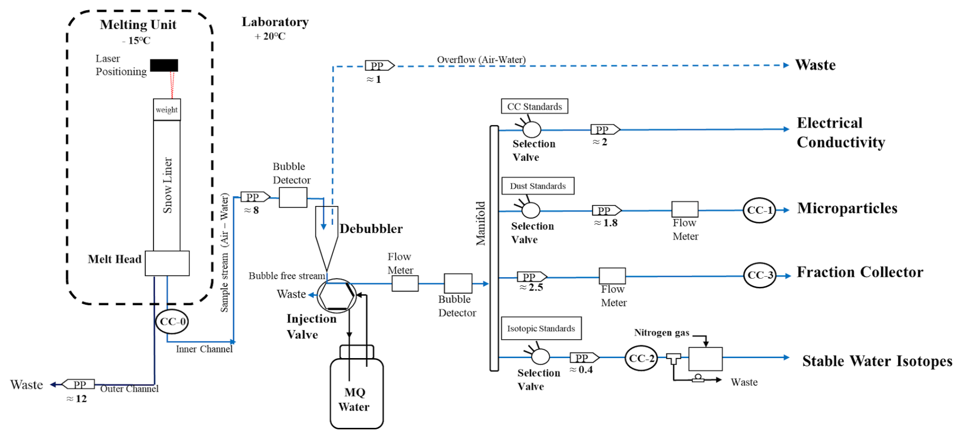
Figure 1 Setup of the AWI CFA system to measure snow cores. The snow core is held in a snow sample holder and melted on a melt head in a −15 °C environment (left-hand side). The laser positioning sensor determines the distance to the weight placed on the top of the core. In the laboratory are the conductivity detectors for synchronization (CC-i), an injection valve switching between MQ water and the snow sample, a degassing unit (debubbler), a manifold, and selection valves for analytical units switching between the sample and standards. The detection of air bubbles takes place upstream and downstream of the debubbler via using bubble detectors. Liquid flow sensors monitor the flow behavior of the system. Finally, peristaltic pumps (PPs) carry the streams from the melt head to all analytical units. All indicated flow values are expressed in mL min⁻¹. A detailed scheme of the water isotopes line is given in Fig. A1.

Melting unit adapted for snow cores

The melting unit for snow cores features a 10 cm inner diameter and 120 cm long tube made of acrylic and positioned centrally above the melt head (Fig. 2a), guiding the sample during the experiment. A light weight (∼150 g) is placed atop of the snow core to stabilize the melt flow and is covered on both sides with a 1 mm thickness layer of polytetrafluoroethylene to prevent contamination. Following the work of Dallmayr et al. (2016), a high-accuracy laser positioning sensor (Way-con, LLD-150-RS232-50-H) determines the distance from the sensor and the top of the weight with a precision of 0.1 mm in order to derive accurate melt speeds and to assign precise depths to the datasets generated.

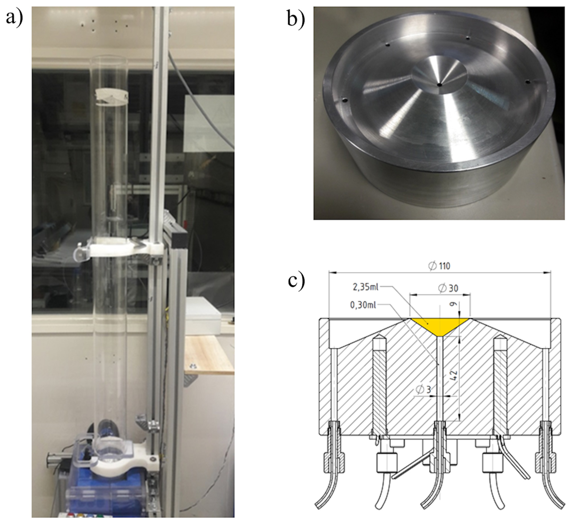
Figure 2 Melting unit. (a) Setup of the snow core melting unit. (b) Picture of the PICE design of the melt head (Kjær et al., 2021). (c) Schematic view of the melt head, showing the dimension of the inner-channel concave volume (orange).

The melt head for snow cores (Fig. 2b) is based on the Physics of Ice, Climate and Earth, (Copenhagen, Denmark, hereafter PICE) design used by Kjær et al. (2021), made of aluminum and manufactured at the AWI in Bremerhaven, Germany. Through a concave volume at the inner-channel (highlighted in Fig. 2c), the shape of the melt head prevents mixing of clean meltwater from the inner part with the potentially contaminated outer part of the core sample. The temperature of the melt head is regulated by a proportional–integral–derivative (PID) temperature controller (Jumo GmbH & Co, Germany) attached to eight 125 W heating cartridges and a conventional thermocouple type J.

Degassing unit

As air in the sample stream leads to significant effects and interferences in the liquid detectors, a separation of air and liquid via a debubbler (Fig. 1) is required. The incoming flow drips into a micropipette opened to the air, releasing the air bubbles to the atmosphere by buoyancy and leading to a bubble-free flow downstream. Furthermore, regarding the inhomogeneous distribution of air bubbles in the incoming flow and unpredictable stops of the core melt, maintaining an amount of water in the debubbler (safety volume) is essential. To that aim, an overflow tube (Fig. 1) connected to a peristaltic pump is continuously sucking air, or an overflow if the water-level within the pipette gets in contact. We set the height of this overflow tube to a minimal safety volume of ∼1 mL. A bubble detector located upstream of the unit (Fig. 1) monitors the variability of air in the incoming stream. A second bubble detector is located downstream of the unit (Fig. 1), monitoring, warning, and recording the detection of air.

Analytical measurements

The CFA system performs the online measurement of electrical conductivity (conductivity cell model 3082, Amber Sciences Inc., USA, Breton et al., 2012) and microparticle counting and sizing (Abakus, Klotz GmbH, Germany, Ruth et al., 2002). Stable water isotope (δ¹⁸O and δD) mixing ratios are continuously measured by a cavity ring-down spectrometer (CRDS; Picarro Inc, USA, Maselli et al., 2013). To obtain the continuity and stability of a micro-flow rate of vapor, as required by the instrument, a stream vaporization module was made based on the original method of Gkinis et al. (2010). A micro-volume tee is used to split a micro-flow into a 50 µm inner diameter fused-silica capillary from the incoming stream. The waste line features a smaller inner diameter. A back pressure is enabled and pushes the micro-flow through the capillary towards the oven, where mixing with dry air occurs before injection to the instrument. To control the back pressure precisely and efficiently, we divided the waste line using a second tee and added a 10-turn micro-metering needle valve to one sub-waste line (Dallmayr et al., 2016). A schematic and technical details of the water isotope line are provided in Appendix A.

In addition to the online measurements, fractions of the melted sample water are carefully collected under a laminar flow bench for further offline measurements of chemical impurities by ion chromatography (normative precision of <10 %, Göktas et al., 2002).

Additional electrical conductivity measurements are performed at the melting unit outlet (CC-0 in Fig. 1, Amber Sciences model 1056, USA) as well as near the inlet of each detection unit (CC-1 to CC-3 in Fig. 1, contactless conductivity measurement, Edaq, Australia). Such duplicated measurements allow for a straightforward and efficient synchronization of the different datasets during data processing (Dallmayr et al., 2016).

Control, data acquisition, and processing

All devices are connected to the controlling computer using software developed with LabVIEW 2012. Drivers are either provided by manufacturers (pumps, flowmeters) or developed to suit the purpose (laser positioning, actuated valves, bubble detectors, all analytical units). Analytical data are recorded every second and are processed after the experiment using a self-made code developed with LabVIEW 2012.

2.2 Assessment of mixing

The determination and the calculation of the mixing of the stable water isotope signal were realized using algorithms developed with R software (R Core Team, 2018).

Characterization of mixing using step functions

CFA systems are known to diffuse, mix, and attenuate the original isotope signal (Gkinis et al., 2011; Jones et al., 2017). The resulting smoothing of the original signal can be described as a mathematical convolution:

$$\begin{array}{}\text{(1)}& {\mathit{\delta }}_{\mathrm{m}}\left(t\right)=[{\mathit{\delta }}_{\mathrm{0}}⊛G]\left(t\right)=\int {\mathit{\delta }}_{\mathrm{0}}\left(\mathit{\tau }\right)G(t-\mathit{\tau })\mathrm{d}\mathit{\tau }\end{array}$$

with δ_m the measured value and δ₀ the original (isotopic) value of the sample at time t. G is a smoothing filter denoting the impulse response of the system, and it refers to the convolution operation.

Here we address the characterization of this mixing by analyzing the impulse response of the system (Fig. 4); i.e., we analyze the derivative of the response of the system to an instantaneous (step) isotopic change. Previously, two approaches were proposed to treat the step response.

First, Gkinis et al. (2011) fit this so-called step response of the system to a scaled cumulative distribution function (hereafter CDF) of a normal distribution, as

$$\begin{array}{}\text{(2)}& {\mathit{\delta }}_{\text{normal}}\left(t\right)={\displaystyle \frac{A}{\mathrm{2}}}\left[\mathrm{1}+\text{erf}\left({\displaystyle \frac{t-t_{\mathrm{0}}}{\mathit{\sigma }\sqrt{\mathrm{2}}}}\right)\right]+B\end{array}$$

with A and B the isotopic values of the step scaled, t₀ the initial time, and σ the standard deviation. All parameters are determined by means of least-squares optimization. In the case of a normal distribution, the impulse response of the CFA system is described by a Gaussian impulse probability density function (hereafter PDF).

$$\begin{array}{}\text{(3)}& G_{\text{normal}}\left(t\right)={\displaystyle \frac{\mathrm{1}}{{\mathit{\sigma }}_{\text{normal}}\sqrt{\mathrm{2}\mathit{\pi }}}}{\mathrm{e}}^{-\frac{(t-t_{\mathrm{0}}{)}^{\mathrm{2}}}{\mathrm{2}{\mathit{\sigma }}_{\text{normal}}^{\mathrm{2}}}}\end{array}$$

Here, the standard deviation of the Gaussian PDF (σ_normal) characterizes the mixing length of the system, expressed in seconds. Later, these values can be converted into a mixing length expressed in millimeters by applying the measured melt speed.

Second, because of the skewed shape of the impulse response, Jones et al. (2017) proposed an implementation from normal CDF to two multiplied lognormal CDFs:

$${\mathit{\delta }}_{\text{log–log}}\left(t\right)={\displaystyle \frac{C}{\mathrm{2}}}\left[\mathrm{1}+\text{erf}\left({\displaystyle \frac{t-t_{\mathrm{1}}}{{\mathit{\sigma }}_{\mathrm{1}}\sqrt{\mathrm{2}}}}\right)\right]\left[\mathrm{1}+\text{erf}\left({\displaystyle \frac{t-t_{\mathrm{2}}}{{\mathit{\sigma }}_{\mathrm{2}}\sqrt{\mathrm{2}}}}\right)\right]+D.$$

This approach provides a slightly better fit to the signal, but the diffusion length is then retrieved using an additional function, fitting the two lognormal CDFs. The derived mixing length thus requires a careful interpretation due to these additional uncertainties.

Our results show very small differences in the resulting mixing lengths obtained by the different approaches (Table 2). We therefore focus this work on the straightforward Gaussian approach to determine diffusion lengths and assess contributions to the overall mixing.

Characterization of mixing by comparison to discrete samples

To evaluate the mixing and the overall performances of the CFA system, we compare the results obtained from CFA with discretely measured samples from the same snow cores. We use six 1 m long snow cores (with the names KF13–KF18), originating from Kohnen station (75°00 S, 0°04 E; 2892 m a.s.l.), Dronning Maud Land (Oerter et al., 2009). This area is characterized by an annual mean temperature of −43 °C (Weinhart et al., 2020) and an accumulation rate of 75 $\mathrm{mm}\mathrm{w}.\mathrm{e}.{\mathrm{yr}}^{-\mathrm{1}}$ over the last 50 years (Moser et al., 2020). The snow cores were taken following the procedure by Schaller et al. (2016) from a trench wall excavated during 2014/2015 (Münch et al., 2017) with a horizontal distance of 5 m. The snow cores were stored in carbon tubes, sealed at each end with plastic bags (Whirl-Pak), and kept inside a Styrofoam box at −25 °C. The 1 m average density of these snow cores ranges between 340–345 kg m⁻³ (Münch et al., 2017). High-resolution density measurements display the layered character of the snow, which induces millimeter–centimeter variations in density and microstructure. However, stable water isotopes do not capture these variations, as the diffusion on site smoothes the signal rather quickly (Moser et al., 2020).

From all snow cores a longitudinal section (slice) of 25 mm thickness was cut. This slice was further cut into discrete subsamples of 22 mm size in vertical resolution. The discrete samples were analyzed at AWI Potsdam in 2015 (hereafter discrete-15). In 2019, a second discrete dataset was obtained with a similar 22 mm depth resolution, just prior to the measurement by CFA. For this second discrete dataset (hereafter discrete-19), four cores (KF13–16) were analyzed for isotopic composition, whereas the remaining two cores (KF17 and 18) were analyzed for ion chromatography at AWI Bremerhaven. For the measurement of the isotopic composition of the discrete-19 dataset, the instruments Picarro L2120-i and Picarro L2130-i were used. The measurement setup followed the Van Geldern protocol (Van Geldern and Barth, 2012). Each sample was injected four times. As a measure of accuracy, we calculated the combined standard uncertainty (Magnusson et al., 2017), including the long-term reproducibility and bias of our laboratory by measuring a quality check standard in each measurement run and including the uncertainty of the certified standards. The combined uncertainty for δ¹⁸O is 0.14 ‰, and for δD it is 0.8 ‰.

3 Results

3.1 Assessing the instrumental performance of the analyzer for stable water isotope measurements

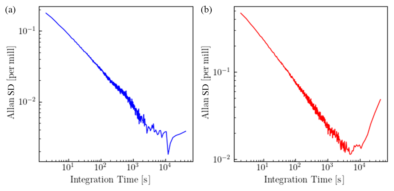
In order to describe the stability and performance of the CRDS instrument for continuous analysis of stable water isotopes, a so-called Allan variance test is applied (Allan, 1966) where over a period of more than 12 h, MQ water is continuously injected at the selection valve for water isotopes (Fig. 1). Such a test allows for the investigation of the noise and drift of the spectrometer with respect to the integration time.

The Allan variance is defined as

$$\begin{array}{}\text{(4)}& A_{\text{var}}={\displaystyle \frac{\mathrm{1}}{\mathrm{2}(n-\mathrm{1})}}\sum _{i=\mathrm{1}}^{n-\mathrm{1}}\left(y\right(\mathit{\tau }{)}_{i+\mathrm{1}}-y(\mathit{\tau }{)}_i{)}^{\mathrm{2}}\end{array}$$

with y(τ) the average value of the measurements during an integration interval of length τ and n being the total number of intervals. The results show the linear decrease in the Allan deviation (square root of Allan variance) up to a minimal deviation for an integration time of ∼6000 s (Fig. 3). Instrumental drift starts slightly earlier than 10⁴ s (Fig. 3), with low deviation (0.01 ‰ for δ¹⁸O and 0.1 ‰ for δD) up to 4×10⁴ s. As one run (melting 1 m liner with CFA) takes up to 2000 s, our measurement time window of this 1 m is well within the non-affected time window for drift. Therefore, one single calibration for each single meter is necessary.

Figure 3 >12 h of Allan deviation analysis for δ¹⁸O (a, in blue) and δD (b, in red).

3.2 Calibration to the VSMOW–SLAP scale and deriving the precision of the continuous dataset

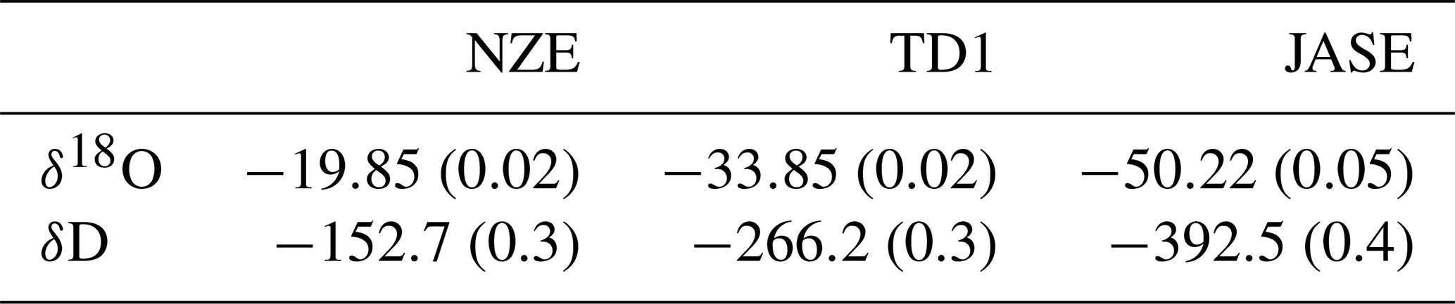
Calibrations of the raw data are performed using three in-house laboratory standards (Table 1), which are annually calibrated to the international VSMOW–SLAP (Vienna Standard Mean Ocean Water–Standard Light Antarctic Precipitation) scale. Each standard is measured for more than 15 min by feeding the CRDS with the standard water via the isotopic selection valve. The values of the last 2 min of each run are averaged. The obtained values are plotted against the defined values; the resulting linear regression fitting the three points is applied and defines the calibration coefficients (Fig. B1, Appendix B).

Table 1 Defined isotopic composition of the in-house laboratory standards used for VSMOW–SLAP calibrations (in ‰). For each standard, the combined uncertainty is given in parentheses.

The precision of the CFA measurements for stable water isotopes is determined from the standard deviation (1 SD) of the last 2 min of each injected standard run. The derived precision from 18 calibration runs (N=18) is 0.24 ‰±0.02 ‰ and 0.47 ‰±0.04 ‰ for δ¹⁸O and δD, respectively.

3.3 Mixing length derived from step function tests

We estimate the mixing length using isotopic liquid standards across different experiments (details given in Table C1 in the supplement). First, during each calibration procedure, three abrupt isotopic changes are applied (dataset CRDS line, Fig. 4) at the water isotope selection valve (Fig. 1). These steps range between ∼100 ‰ and ∼140 ‰ (Appendix C) and show no dependency between isotopic step size and diffusion length. In a second experiment, we applied an isotopic step (∼230 ‰) at the melt head, with its concave volume filled (MH-filled dataset, Fig. 4). Finally, the same step was then applied with the concave volume empty (MH-empty dataset, Fig. 4).

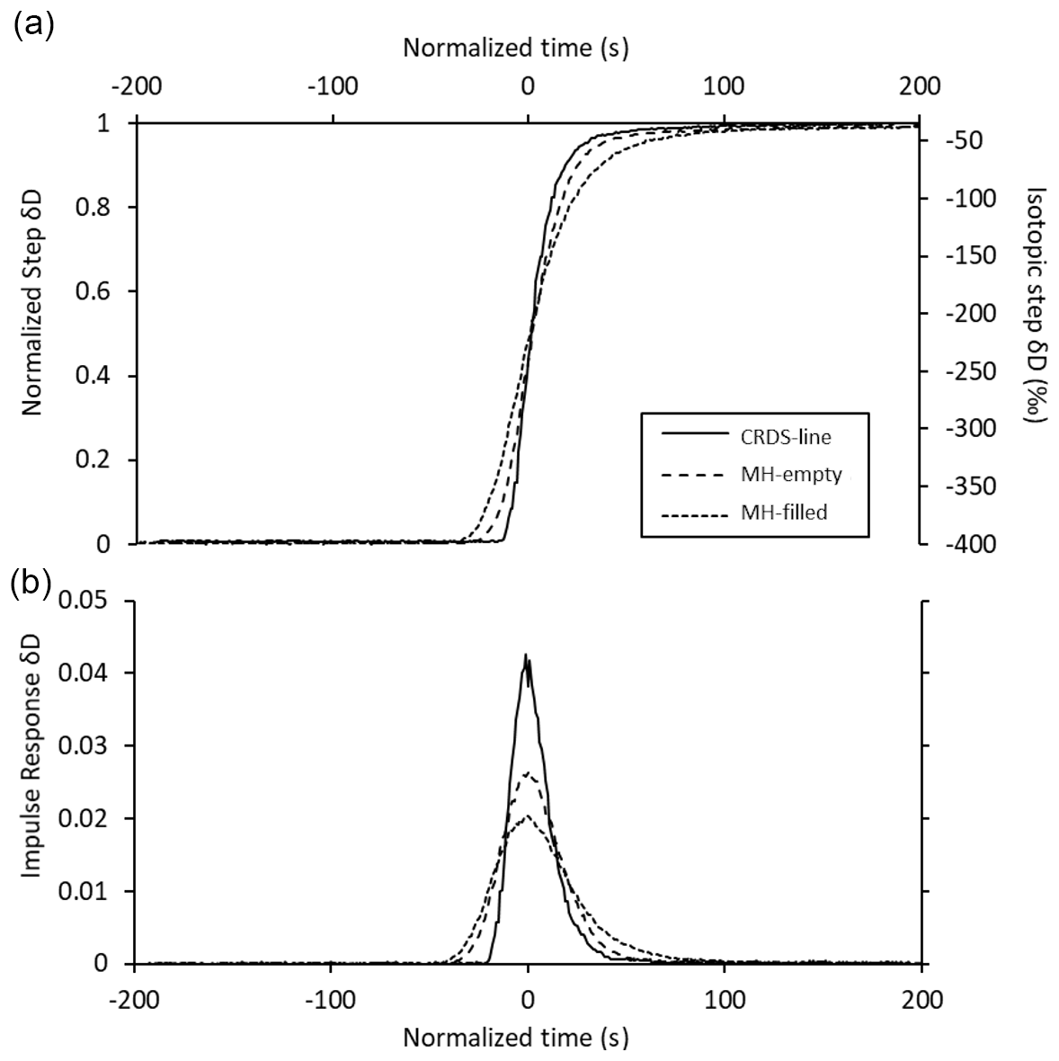
Figure 4 Isotopic step and impulse responses obtained for the three experiments realized. (a) The different normalized step functions. (b) The corresponding impulse responses.

Using Eqs. (1)–(3), we compute the mixing lengths (σ) of our set of experiments (σ_MH-filled, σ_MH-empty, σ_{CRDS line}). The results for both isotopologues δD and δ¹⁸O are very similar (Appendix C, Table C2), consistently showing a slightly longer diffusion length for δD. Therefore, we focus our study on the results for δD (Table 2). Furthermore, in addition to evaluating the mixing length induced by the whole CFA system, the combination of the three datasets allows us to distinguish between the contributions of the different parts of the system. Assuming independent mixing from each other from the melt head (MH) to the water isotope selection valve (WI-SV) and later to the CRDS instrument, the total mixing filter is the sum of the variances of each mixing filter along the CFA system.

$$\begin{array}{ll}{\displaystyle }{\mathit{\sigma }}_{\text{CFA system}}^{\mathrm{2}}& {\displaystyle }={\mathit{\sigma }}_{\text{MH-filled}}^{\mathrm{2}}\\ \text{(5)}& {\displaystyle }& {\displaystyle }={\mathit{\sigma }}_{\text{MH}}^{\mathrm{2}}+{\mathit{\sigma }}_{\text{MH to WI-SV}}^{\mathrm{2}}+{\mathit{\sigma }}_{\text{CRDS line}}^{\mathrm{2}}\end{array}$$

We can evaluate by quadrature difference (1) the mixing length induced by the concave volume of the melt head (${\mathit{\sigma }}_{\text{MH}}=\sqrt{{\mathit{\sigma }}_{\text{MH-filled}}^{\mathrm{2}}-{\mathit{\sigma }}_{\text{MH-empty}}^{\mathrm{2}}}$) and (2) the mixing length induced downstream of the melt head to the isotopic selection valve (${\mathit{\sigma }}_{\text{MH to WI-SV}}=\sqrt{{\mathit{\sigma }}_{\text{MH-empty}}^{\mathrm{2}}-{\mathit{\sigma }}_{\text{CRDS line}}^{\mathrm{2}}}$).

Table 2 δD mean mixing lengths derived from the skew and normal PDFs, expressed in seconds (italic) and in millimeters (bold). Values in parentheses represent 1 SD. The conversion of seconds to millimeters is based on a melt speed of 38 mm min⁻¹. σ_MH and σ_{MH to WI-SV} correspond to differences in quadrature between σ_MH-filled and σ_MH-empty and between σ_MH-empty and σ_{CRDS line}, respectively.

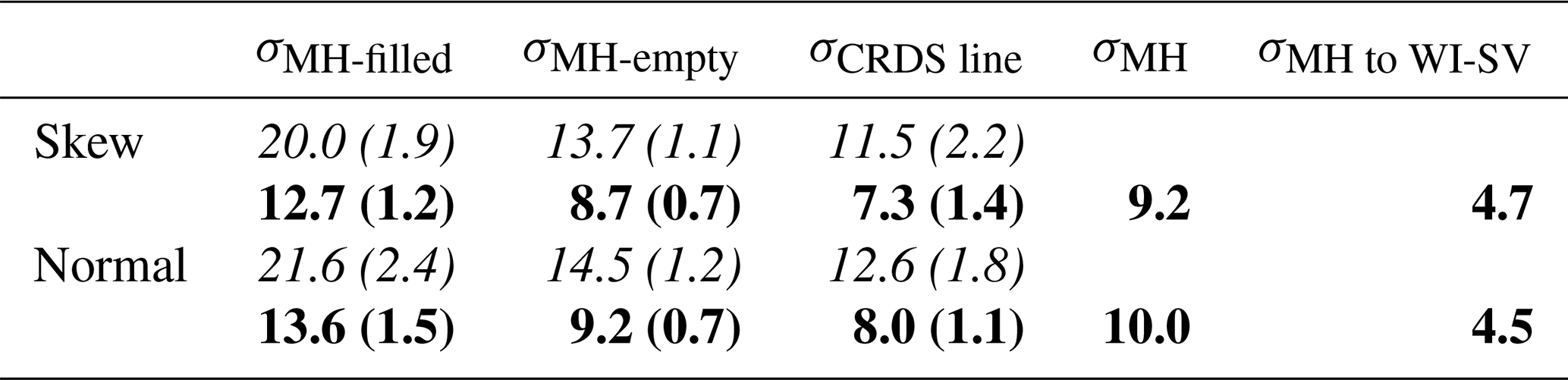
We find a total mixing length of the AWI CFA system of ∼14 mm (Table 2), indicating that the majority of the instrumental mixing is induced by the concave volume of the PICE design melt head (10 mm mixing length), closely followed by the CRDS line (8 mm). The tubular section in between, composed of tubes and the ∼1 mL safety volume of the debubbler, shows a significantly smaller contribution (4.5 mm).

3.4 Snow-core continuous records versus discrete records

3.4.1 Mixing length derived from comparison to discrete measurements

We compare the discrete values from 2015 and 2019 as well as the values obtained from CFA at the single profiles (Fig. 5, upper panel) as well as at the mean profile, averaged over all profiles (Fig. 5, bottom) and quantify the differences. We first observe a mismatch in the depth assignment between discrete and CFA values; i.e., the phase of the records has an offset of 12.3±6.4 mm. One reason for the mismatch could be the short-term fluctuation in the melt speed induced by density variations. However, the melt speed is measured with high resolution, and variations are included in the depth assignment. We therefore assume that the depth assignment from CFA is quite accurate. On the other hand the depth assignment of the discrete samples is less accurate, as the subsampling generates uncertainty in the exact size and position of each sample (i.e., loss of material due to the cutting). This uncertainty in the depth assignment and the corresponding matching to the CFA data may be one major reason for the observed mismatch of discrete and continuous data. Secondly, comparing the amplitude between isotopic minima and maxima show that the continuous record attenuates on average ∼17 % of the discrete-19 record and ∼48 % of the discrete-15 record. The strong difference between the two discrete datasets reveals a further and significant diffusional process occurring likely during the storage of the snow cores (Van der Wel et al., 2011). Therefore, we use the discrete-19 dataset to assess the effect of percolation, while the offset between the two discrete datasets is discussed later as an indicator of diffusion during storage (see Sect. 4, Discussion).

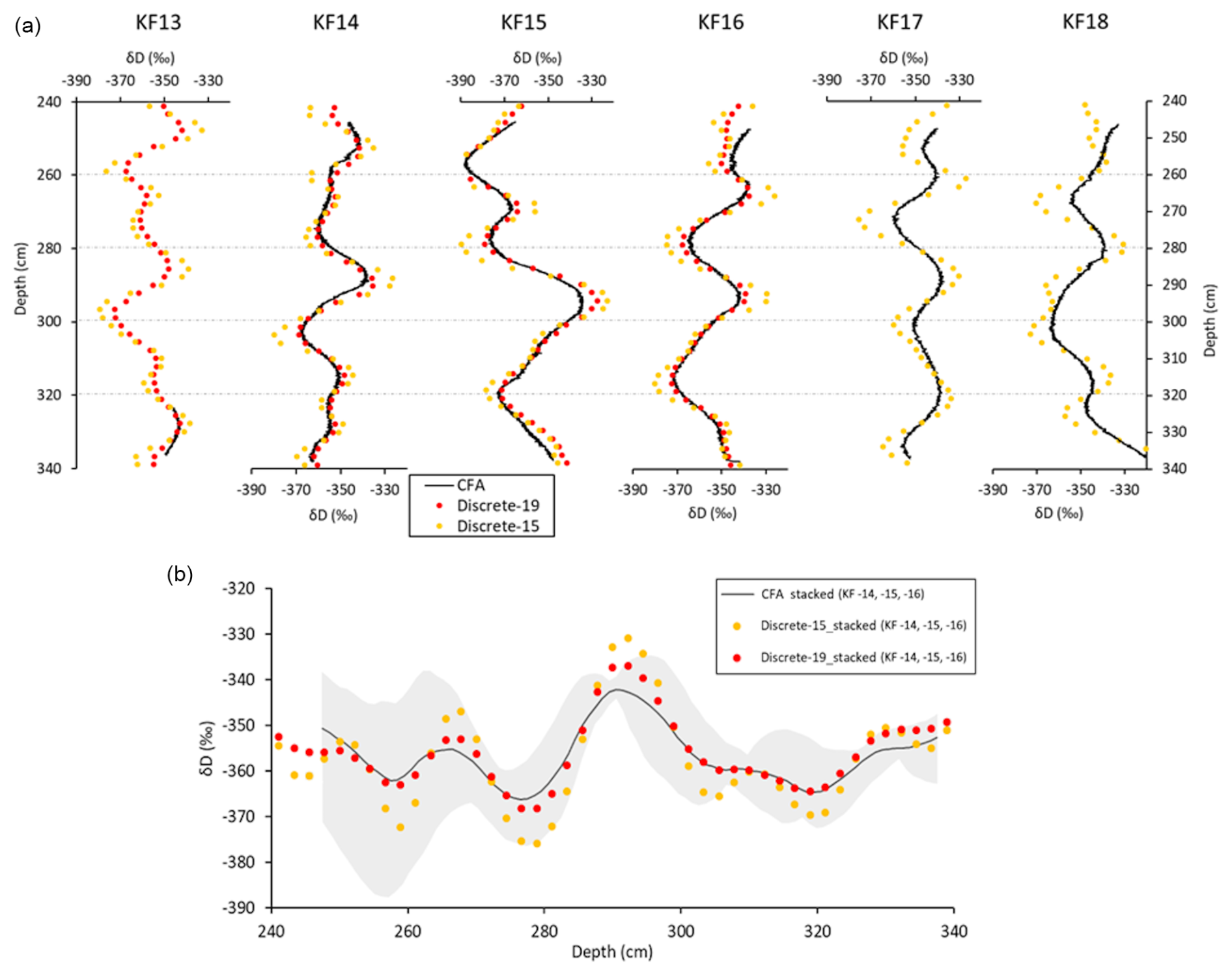
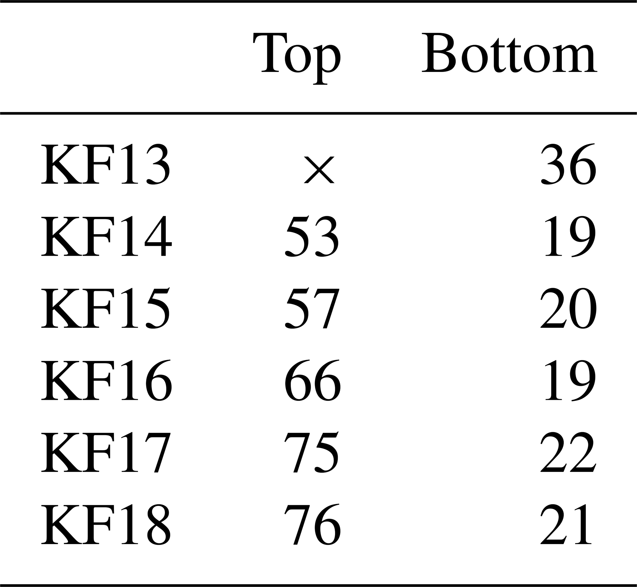
Figure 5 Isotope profiles of the six snow cores. (a) 240–340 cm depth δD profiles of the six cores, 5 m spaced. Continuous measurement (black lines), discrete-15 (orange markers), and discrete-19 (red markers) datasets are shown. Note the small 150 mm portion of reliable continuous analysis for the core KF13, due to issues during the run. Because of the transition from MQ to sample and vice versa, we removed the top 65 (±10) mm and bottom 20 (±1.3) mm of the continuous datasets KF14–18 (details of the exact removed data are given in Table E1, Appendix E). The averaged melt speed of the six runs is 38 mm min⁻¹ ($\mathrm{1}\text{SD}=\mathrm{9}\mathrm{mm}{\min }^{-\mathrm{1}}$). (b) Mean datasets of the stacked CFA (black) and discrete (dotted) profiles of the snow cores KF14, KF15, and KF16. The gray shaded area displays the spread of the three CFA profiles.

3.4.2 Separating the effect of percolation from the overall mixing

When continuously analyzing a snow core, due to the high-porosity of the upper-meters samples, capillary action (Colbeck, 1974) forces the melted water at the MH to lift upwards, enabling percolation (Fig. 6). Thus, by comparing the continuous dataset with a percolation-free discrete dataset, we aim to assess the mixing induced by the percolation.

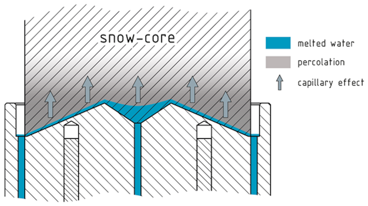
Figure 6 Illustration of the melting experiment showing the percolation induced by the low density of the sample combined to the melt-water reservoir within the inner concave volume of the melt head.

In order to retrieve the mixing length induced by the continuous analysis of snow cores with respect to the discrete dataset, we convolved the discrete signal with a family of impulse responses of different mixing lengths. A set of discrete-convolved signals of flattened extrema are obtained, and each signal is compared to the CFA signal (previously smoothed on 22 mm to ensure the same averaging than the discrete samples). Then, the minimum of root mean square ($\text{rms}=\sqrt{\text{mean}\left(\right(x_i-x_j{)}^{\mathrm{2}})}$) between convolved signals and the continuous record allows for the identification of the adequate mixing length σ_CFA-discrete.

Table 3 Mixing lengths (in mm) of the continuous profiles of δD, as related to the discrete-19 dataset and to the discrete-15 dataset. No results are available for the KF13 core due to the too short continuous dataset.

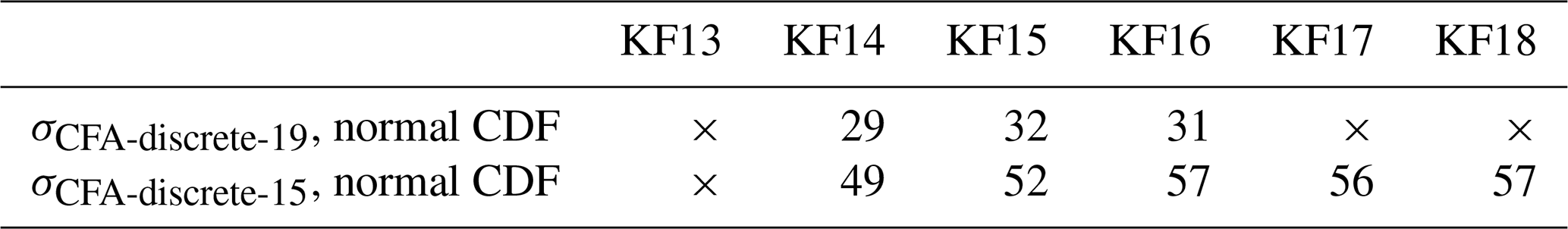
We find average mixing lengths of approximately 30 mm for the discrete-19 dataset and 54 mm for the discrete-15 dataset (Table 3). Following Eq. (5), we separate the mixing from the percolation at the melt head from the remaining CFA system by the following equation.

$$\begin{array}{}\text{(6)}& {\mathit{\sigma }}_{\text{CFA-discrete-19}}^{\mathrm{2}}={\mathit{\sigma }}_{\text{CFA system}}^{\mathrm{2}}+{\mathit{\sigma }}_{\text{percolation}}^{\mathrm{2}}\end{array}$$

σ_{CFA-discrete-19} refers to the overall mixing retrieved from the convolution of the discrete-19 signal. σ_{CFA system} is the observed mixing of 14 mm of the CFA system derived from experiments with the step function (Sect. 3.3).

By retrieving the quadratic difference of the CFA-discrete-19 and CFA system, we can compute the mixing length induced by the percolation at the melt head with ∼27 mm. This length is twice the length induced by the experimental system. Thus, percolation is the limiting factor on retrieved signal resolution when applying CFA on snow cores.

4 Discussion

The need to address local spatial noise in the stable water isotope ice core records from low-accumulation rate areas such as Kohnen station, Dronning Maud Land, with an accumulation rate of 200–300 mm recent annual gain of snow (Münch et al., 2017) motivates analysis of low-density snow cores with less effort compared to discrete sampling. In order to assess the ability of a CFA system to analyze these very low density (e.g., $<\mathrm{400}\mathrm{kg}{\mathrm{m}}^{-\mathrm{3}}$, Laepple et al., 2016) cores, here we used an adapted melting unit of the CFA system to analyze in total six snow cores from Kohnen station. We find a good agreement between the different isotope profiles of the different snow cores. The derived mixing length of the CFA system with respect to the isotopic signal is found to be similar to the improved CFA–CRDS system at the University of Colorado (mixing length for δD of 21.6 s, Sect. 3.3 of this work, versus 19.1 s, Jones et al., 2017). These agreements in derived mixing lengths indicate, together with our quantitative estimates (Table 2), that a major contribution to the mixing is inherent in the usage of the Picarro instrument (CRDS line).

4.1 Suggestion to address the percolation

The largest contribution originates from the percolation at and above the melt head. We assign the percolation to the design of the melt head and its large inner concave volume (Fig. 2). To overcome the high level of mixing induced by the percolation, it is crucial to prevent the formation of a reservoir of meltwater in contact with the snow core, specifically in the inner volume at the melt head. Thus, a new design of inner channel offers a possibility towards this aim. A flat surface covered with boreholes will allow for an efficient and uniform evacuation of the meltwater, limiting the suction upward. In addition to addressing the percolation, such design will significantly increase the experimental performances (Sect. 3.3) in order to ultimately offer the necessary quality to resolve reliably the full isotopic cyclicity in the snowpack in low-accumulation-rate areas.

The significant contribution of the Picarro analyzer to the mixing length of the CFA system (CRDS line, Sect. 3.3) could be addressed as well and requires likely a collaboration with the manufacturer to improve the analytical unit itself (e.g., reduction of the large volume at its inlet before a pressure drop to the 40 Torr cavity).

4.2 The effect of variations of melt speed on the mixing length

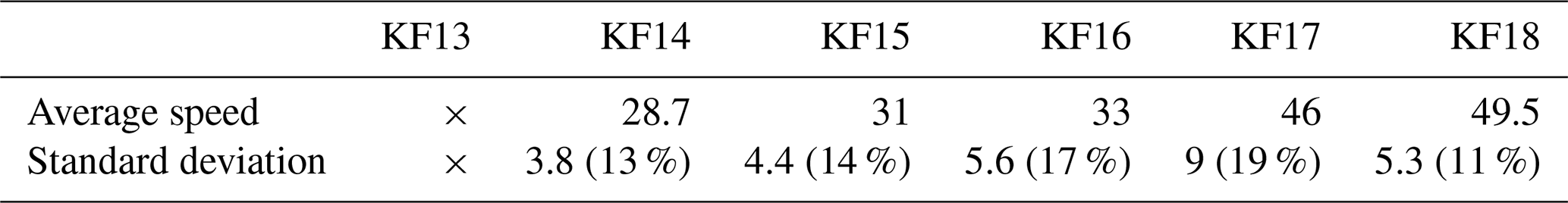
Further we explored the sensitivity of mixing length to melt speed. We melted the snow cores at different melt speeds, varying from 28.7 to 49.5 mm min⁻¹ (Table 4). As the obtained mixing lengths do not show any trend (see Table 3), we are confident that the mixing length is not sensitive to melt speed variations. We however observed variability of melt speed within each core between 10 % and 20 % of the mean speed (Table 5), which can be related to small-scale variations of snow density or friction within the sample holder.

Table 4 Melt speed statistics for the different snow cores, expressed in mm min⁻¹. The upper row shows the averaged melt speed of each run, while the lower row indicates the corresponding variability (standard deviation observed, in mm min⁻¹), and in parentheses as a percentage of the mean value.

4.3 Spatial variability

The six firn cores were taken in the vicinity of Kohnen station with a distance of 5 m. Their different profiles display stratigraphic noise, i.e., spatial variability. The variability in the isotope profiles due to this spatial variability is in the range or larger (Fig. 5, lower panel) than the error obtained due to the mixing by the CFA, i.e., the reduced amplitudes compared to discrete data or delay in the signal compared to the discrete data. This strengthens the potential of using CFA to analyze many snow cores of one site to generate an average isotope profile (Münch et al., 2017).

4.4 Diffusion of the isotope signal during storage of snow cores

From comparing the CFA data with discrete measurements (Fig. 5), we observed a significant difference between the stable water isotopic profiles of the same snow cores sampled at different times.

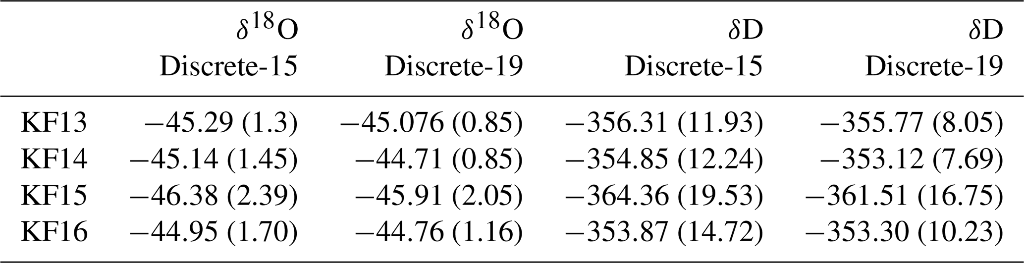
Table 5 δ¹⁸O and δD means (standard deviation) for each snow core discrete dataset, expressed in units of per mill (‰).

This difference is not related to instrumental induced mixing but instead indicates the effect of long-term storage of snow samples. We assume that diffusion, known to occur in snow and firn (Gkinis et al., 2014), also occurs in the cold storage environment. Using our results, we can now quantity this storage-induced diffusion. Assuming that the mixing of the discrete-15 dataset corresponds to the mixing of the discrete-19 dataset convolved with an independent smoothing filter induced by the storage yields the following equation.

$$\begin{array}{}\text{(7)}& {\mathit{\sigma }}_{\text{CFA-discrete-15}}^{\mathrm{2}}={\mathit{\sigma }}_{\text{CFA-discrete-19}}^{\mathrm{2}}+{\mathit{\sigma }}_{\text{storage 15–19}}^{\mathrm{2}}\end{array}$$

Using the calculated mean mixing lengths σ_{CFA-discrete-19}=30 mm and σ_{CFA-discrete-15}=54 mm (Table 3), we derive a diffusion length of approximately 45 mm. These findings indicate that during the 4 years of storage (from the first analysis in 2015 to the second analysis in 2019), the isotope signal in the snow cores was smoothed by this diffusion length.

Additionally, we computed the mean and variability (standard deviation) of both discrete datasets for each 1 m long snow core (Table 5). The decrease in amplitude indicates an average attenuation of 0.54 ‰ and 4.5 ‰ for δ¹⁸O and δD, respectively. The mean values show on average an enrichment of isotopic composition of +0.31 ‰ for δ¹⁸O and +1.6 ‰ for δD, likely due to the repeated contact with laboratory air when bags are opened and the loss of sample (frost) in the bag.

We show the effect of storage on diffusion lengths for both isotopologues (Fig. D1, Appendix D) based on firn diffusion model (Gkinis et al., 2014). The model run assumes a storage temperature of −20 °C, a density of 370 kg m⁻³, and an accumulation rate of 75 $\mathrm{mm}\mathrm{w}.\mathrm{e}.{\mathrm{yr}}^{-\mathrm{1}}$ (even though there is no accumulation during storage). For a time window of 4 years, we found a diffusion length for δD similar to our observations (Fig. D1). As the diffusivity coefficients are positively correlated to temperature, the diffusion during storage is likely of stronger magnitude than on the East Antarctic plateau (Fig. D2, Appendix D). However, the strength of the observed diffusion during storage is due to the low density of the snow cores, and we do not expect such a strong change for firn and ice core samples from greater depth and with higher density.

5 Conclusions

To overcome the increased stratigraphic noise in low-accumulation areas and constrain the isotope signal formation within the upper firn, a large number of high-quality stacked vertical profiles is required (Münch et al., 2017). In order to cope with the related challenge of high-pace quality analysis and paired measurements of various proxies, here we present a CFA system adapted for analysis of snow cores using a previously designed melt head for snow cores (Kjær et al., 2021). Based on standard step functions and mathematical approaches (Gkinis et al., 2011, Jones et al., 2017), we quantify the mixing of the isotopic signal induced by the CFA system and separate the different contributors. As a result, we identify percolation (especially strong due to the low density) at and above the melt head as a major contributor to the overall mixing of the isotope record. Despite these limitations we show that CFA can be used to obtain reasonable isotope profiles of snow cores, keeping information on both the spatial and temporal variability. However, for future applications of CFA to snow cores, we recommend a new design of the melt head, with a focus on the evacuation of the meltwater. Finally, the isotopic diffusion during storage of snow-core samples requires further investigation but underlines the need of (1) a strategy to preserve the original record (discrete samples cut in the field) or (2) prompt analysis with techniques such as CFA.

Appendix A: CFA water isotope line

The selected sample steam is drained at a flow of $\sim \mathrm{0.2}\mathrm{mL}{\min }^{-\mathrm{1}}$ through PFA tubes of 0.51 mm inner diameter to a 10 µm frit filter (A-107, Idex) and then a synchronization conductivity cell before entering a stainless-steel micro-volume tee (U-428, Idex; T1 in Fig. A1). Here, a micro-flow is split from the incoming stream into a fused-silica capillary tube (50 µm inner diameter), and the rest goes into the waste line. Due to the smaller inner diameter of the waste line (0.25 mm), a back pressure pushes the micro-flow through the capillary towards the oven. To control this back pressure precisely and efficiently, the waste line is divided using a polyether ketone tee (T3) and then added a 10-turn micro-metering needle valve to one of the two sub-waste lines (P-445, Idex).

The sample micro-flow is injected into the stainless-steel tee (T2, Valco ZT1M) mounted in the 180 °C oven, where it vaporizes instantly and mixes with a controlled flow of dry air (mass flow controller SEC-E40 N2 100SCCM, Horiba company) to form a gas sample with the desired water vapor concentration.

Figure A1 Detailed schematic of water isotope line of the AWI CFA system.

Appendix B: Three-point calibration to the VSMOW–SLAP scale and accuracy

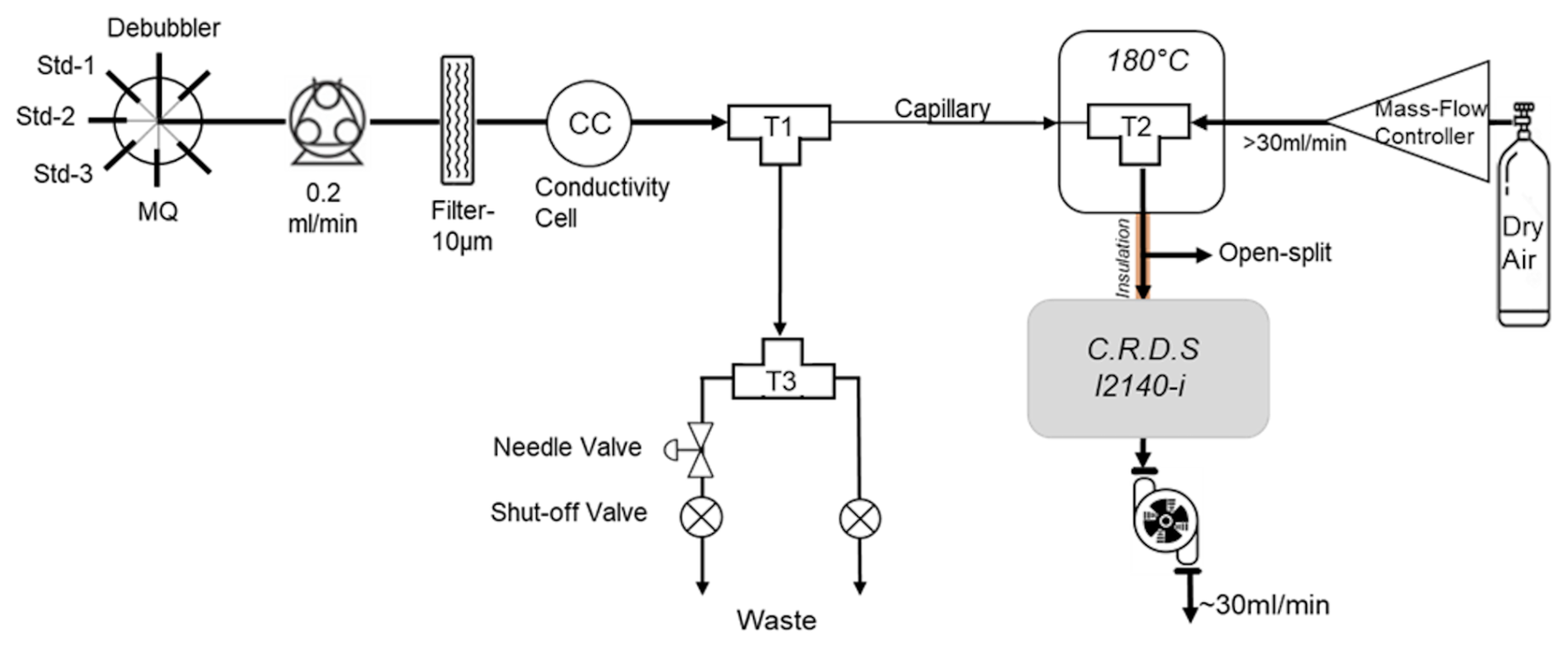
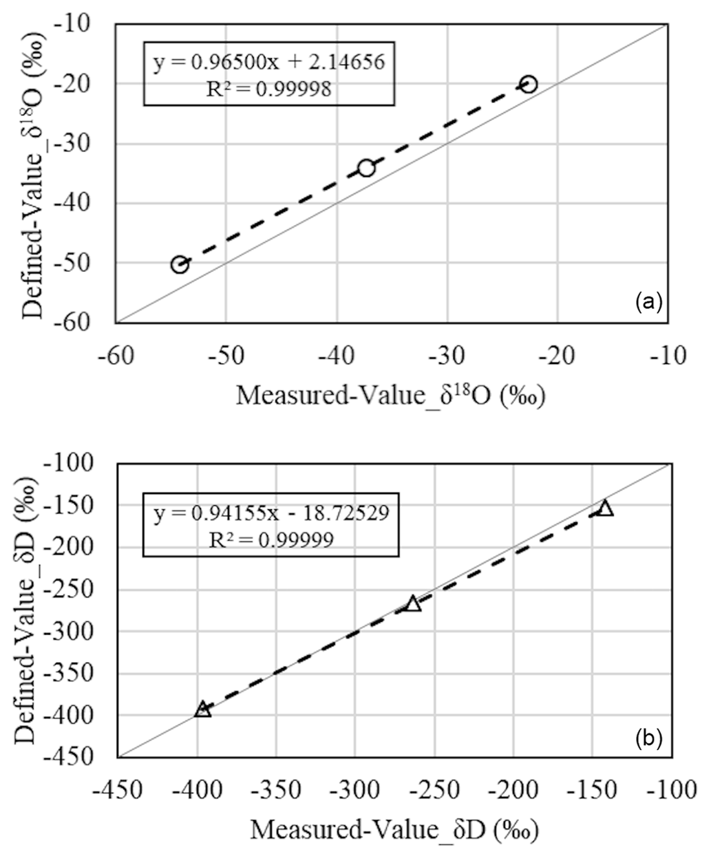
Figure B1 VSMOW–SLAP three-point calibration with in-house laboratory standards NZE, TD1, and JASE. (a δ¹⁸O, b δD). The thin gray line is the 1:1 line. Data points are raw data, i.e., before calibration.

Table B1 Deviations between calibrated and defined values. All values are expressed in units of per mill (‰).

Appendix C: Mixing length derived from step function tests

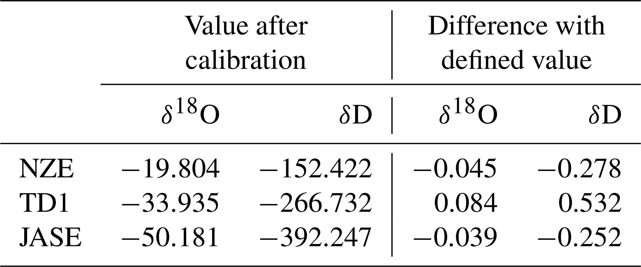
Table C1 Details of the different experiments conducted to assess the overall instrumental mixing and separating the different contributions along the setup.

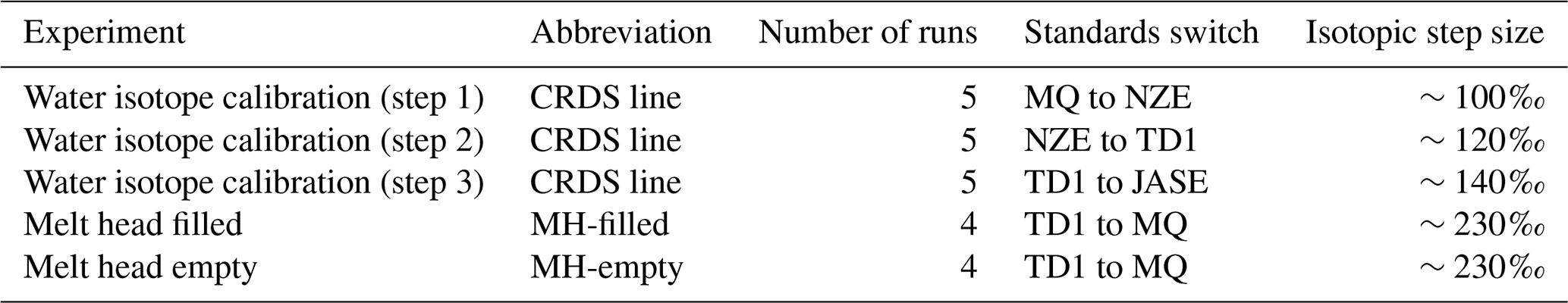
Table C2 Mean mixing lengths derived from the skew and normal PDFs, expressed in seconds (italic) and in millimeters (bold) for both δ¹⁸O and δD. Values in parentheses represent 1 SD. The conversion of seconds to millimeters is based on a melt speed of 38 mm min⁻¹. σ_MH and σ_{MH  to  WI-SV} correspond to differences in quadrature between σ_MH-filled and σ_MH-empty and between σ_MH-empty and σ_{CRDS line}, respectively.

Appendix D: Firn diffusion during storage

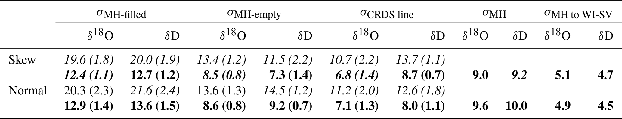
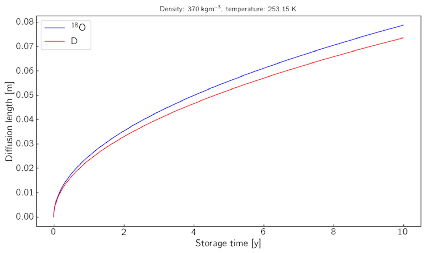
Figure D1 Exemplary firn diffusion length estimates for firn samples with a density of 370 kg m⁻³ as a function of storage time. The firn diffusion length is computed based on the model by Gkinis et al. (2014), using a temperature of −20 °C and an accumulation rate of 75 $\mathrm{mm}\mathrm{w}.\mathrm{e}.{\mathrm{yr}}^{-\mathrm{1}}$.

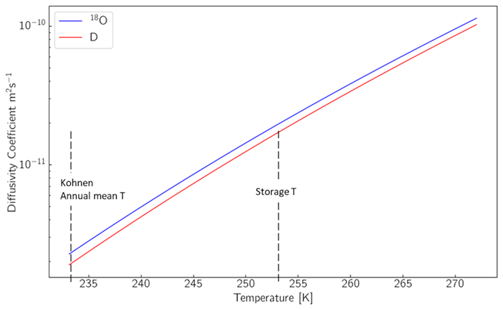
Figure D2 Diffusivity coefficients versus temperature (constraints as above). The annual mean temperature at Kohnen station (−43 °C, Weinhart et al., 2020) and the storage temperature (−20 °C) are displayed.

Appendix E: Data removed from continuous datasets

Table E1 Data removed from the top (left column) and the bottom (right column) of the continuous datasets due to the transition with MQ water (expressed in mm).