the Creative Commons Attribution 4.0 License.
the Creative Commons Attribution 4.0 License.
 | 01 Mar 2024
Effects of Arctic sea-ice concentration on turbulent surface fluxes in four atmospheric reanalyses
Tereza Uhlíková
Timo Vihma
Alexey Yu Karpechko
Petteri Uotila
A prerequisite for understanding the local, regional, and hemispherical impacts of Arctic sea-ice decline on the atmosphere is to quantify the effects of sea-ice concentration (SIC) on the turbulent surface fluxes of sensible and latent heat in the Arctic. We analyse these effects utilising four global atmospheric reanalyses, ERA5, JRA-55, MERRA-2, and NCEP/CFSR (including both the NCEP Climate Forecast System Reanalysis (CFSR) and the NCEP Climate Forecast System Version 2 (CFSv2)), and evaluate their uncertainties arising from inter-reanalysis differences in SIC and in the sensitivity of the turbulent surface fluxes to SIC. The magnitude of the differences in SIC is up to 0.15 but typically around 0.05 in most of the Arctic over all four seasons. Orthogonal-distance regression and ordinary-least-squares regression analyses indicate that the greatest sensitivity of both the latent and the sensible heat flux to SIC occurs in the cold season, November to April. For these months, using daily means of data, the average sensitivity is 400 W m−2 for the latent heat flux and over 800 W m−2 for the sensible heat flux per unit of SIC (change in SIC from 0 to 1), with differences between reanalyses that are as large as 300 W m−2 for the latent heat flux and 600 W m−2 for the sensible heat flux per unit of SIC. The sensitivity is highest for the NCEP/CFSR reanalysis. Comparing the periods 1980–2000 and 2001–2021, we find that the effect of SIC on turbulent surface fluxes has weakened owing to the increasing surface temperature of sea ice and sea-ice decline. The results also indicate signs of a decadal-scale improvement in the mutual agreement between reanalyses. The effect of SIC on turbulent surface fluxes arises mostly via the effect of SIC on atmosphere–surface differences in temperature and specific humidity, whereas the effect of SIC on wind speed (via surface roughness and atmospheric-boundary-layer stratification) partly cancels out in the turbulent surface fluxes, as the wind speed increases the magnitudes of both upward and downward fluxes.
- Article
(8829 KB) - Full-text XML
- Companion paper
-
Supplement
(28910 KB) - BibTeX
- EndNote


Interactive processes within the air–ice–ocean system play a key role in the rapid Arctic warming of the lower troposphere and sea-ice decline (Dai et al., 2002; Screen and Simmonds, 2010; Serreze et al., 2009). These processes are complex and challenging to represent in models; yet, to better understand the local, regional, and hemispherical impacts of Arctic sea-ice decline on the atmosphere, it is crucial to quantify the effects of sea-ice concentration (SIC) on turbulent surface fluxes in the Arctic.
The surface mass balance of sea ice (bare or snow covered) is controlled by the solar short-wave and thermal long-wave radiative fluxes, the turbulent surface fluxes of latent and sensible heat (LHF, SHF), and the conductive heat flux from the ocean through ice and snow. According to observations, in winter, the cooling of the snow/ice surface due to negative net long-wave radiation is balanced by the downward SHF from air to ice and the upward conductive heat flux (Persson et al., 2002; Walden et al., 2017). By warming the snow/ice surface, SHF reduces the temperature gradient through the ice and snow and, accordingly, reduces the basal ice growth (Lim et al., 2022). In spring, the downward long-wave radiation is usually the most important factor triggering the onset of snowmelt on top of sea ice (Maksimovich and Vihma, 2012), whereas in summer, the downward solar radiation is mostly responsible for the surface melt of snow and ice (Tsamados et al., 2015).
Sea ice affects the climate system by regulating the exchange of momentum, heat, moisture, and other material fluxes between the atmosphere and the ocean and by having a much higher albedo than the open water. The difference in albedo between the sea ice and the ocean plays the most significant role during summer, when the sun is at its highest and the reduced albedo of the sea-ice-free water allows more absorption of the downward solar radiation that heats the ocean and, via the turbulent fluxes, the near-surface air (Perovich et al., 2007). The insulating effect of the sea ice is especially evident during winter and spring, when the ocean is considerably warmer than the atmosphere. Then the heat loss to the atmosphere mostly occurs in areas of open water: leads and polynyas. Leads are narrow, elongated openings of the ice cover typically generated by divergent ice drift, and they may be several tens of kilometres long and metres to kilometres wide (Alam and Curry, 1997). Polynyas are larger areas of open water generated by either sea-ice dynamics or an anomalous oceanic heat flux that melts the ice from below (Wei et al., 2021). The heat loss from leads and polynyas to the atmosphere is mostly governed by SHF, with LHF and net long-wave radiation playing smaller roles (Gultepe et al., 2003). The magnitude of upward LHF and SHF over these sea-ice openings is often 10 to 100 times larger than that over the sea ice (Overland et al., 2000; Michaelis et al., 2021), and wintertime observations have indicated that the sum of SHF and LHF exceeds 500 W m−2 (Andreas et al., 1979). Hence, variations and climatological trends in SIC are critically important for the heat budget of the lower atmosphere and the upper ocean in the Arctic, and a key issue is to better understand and quantify the interactions of SIC and the surface turbulent fluxes.
From the point of view of modelling the atmosphere, sea ice is a challenging surface type. SIC may change rapidly due to the combined effects of dynamic and thermodynamic atmospheric and oceanic forcing (Aue et al., 2022). Due to these rapid changes and the challenges presented by sea-ice monitoring due to the darkness during the polar night and prevailing cloud cover during summer, the information available on SIC is often inaccurate. Because of the optical challenges of sea-ice monitoring, the information is mostly based on passive microwave remote-sensing data from polar-orbiting satellites. However, as shown, e.g. in Fig. 7 in Valkonen et al. (2008), the same passive microwave data processed using different algorithms may result in differences on the order of 20 %, which adds to the uncertainty in the representation of the Arctic lower atmosphere in models.
Nevertheless, global atmospheric reanalyses provide the best available information in data-sparse regions such as the Arctic (Bosilovich et al., 2015; Gelaro et al., 2017; Kobayashi et al., 2015) and are often relied upon in climate and climate-change research. These data sets aim to provide a physically consistent estimate of past states of the atmosphere with spatial and temporal resolutions that are uniform around the globe, and they are generated by assimilating atmospheric and surface observations with short-term weather forecasts using modern weather-forecasting models. While the differences in SIC, LHF, and SHF between reanalyses have been demonstrated via comparisons against observations (Bosilovich et al., 2015; Graham et al., 2019) and inter-comparisons between reanalyses (Collow et al., 2020; Graham et al., 2019; Lindsay et al., 2014), how much different reanalyses vary in the relationships between SIC and surface turbulent fluxes is not known. To fill these knowledge gaps, we carry out an inter-comparison of four commonly used major global atmospheric reanalyses: ERA5, JRA-55, MERRA-2, and NCEP/CFSR (including both the NCEP Climate Forecast System Reanalysis (CFSR) and the NCEP Climate Forecast System Version 2 (CFSv2)), with a focus on the relationships between SIC, LHF, and SHF within each reanalysis.
The study region is the marine Arctic. We used data from the era of satellite measurements (1980–2021), as, compared to previous years, they provide more reliable and consistent information on the concentration of Arctic sea ice, which in turn also allows for more precise estimation of turbulent surface fluxes in reanalyses. The past 42 years was divided into two study periods: 1980–2000 and 2001–2021. According to HadCRUT5 data (Morice et al., 2021), the Arctic has warmed more than the world during most years since 1980, though the Arctic amplification phenomenon strengthened considerably shortly after 2000. Hence, the division into two study periods allowed us to compare the period of recent strong Arctic amplification of climate warming to the period directly preceding this phenomenon. Each year was divided into four 3-month seasons with regard to the annual cycle of the Arctic sea ice: (1) November–December–January, (2) February–March–April, (3) May–June–July, and (4) August–September–October. November–December–January represents the months of high sea-ice extent, February–March–April represents the months preceding and following the maximum sea-ice extent in March, February–March–April represents the months of low sea-ice extent, and August–September–October represents the months surrounding the month of minimum sea-ice extent in September.
We worked with data from four reanalyses: ERA5 (Hersbach et al., 2023), JRA-55 (Japan Meteorological Agency, 2013), MERRA-2 (GMAO, 2015a, b), and NCEP/CFSR (Saha et al., 2010b, 2011), all covering the selected period 1980–2021. Under the term “NCEP/CFSR”, we included data from the NCEP CFSR (covering the period 1980–2010) and NCEP CFSv2 (covering the period 2011–2021). Because these two data sets come with different horizontal spatial resolutions (0.312° × 0.313° vs. 0.204° × 0.205°), we unified them using bilinear interpolation to give a resolution of 0.4° × 0.4° (∼45 km grid cell) for the whole NCEP/CFSR data set. Except for this adjustment, we worked with the original horizontal spatial resolutions of the remaining reanalyses, which vary from ∼31 to ∼55 km (ERA5 vs. JRA-55). The update cycle for the reanalysis forecasts (temporal resolution) ranges from 1 to 6 h (ERA5 and MERRA-2 vs. NCEP/CFSR). In our study, we used daily means of the data, as they provide a sufficient representation of synoptic-scale atmospheric and sea-ice processes for our needs while significantly decreasing the size of the data set. For an overview of the basic characteristics of the reanalyses, see Table 1.
Hersbach et al. (2020)Kobayashi et al. (2015)Gelaro et al. (2017)Saha et al. (2010a)Saha et al. (2014)Table 1Basic characteristics of the utilised global atmospheric and coupled reanalyses.
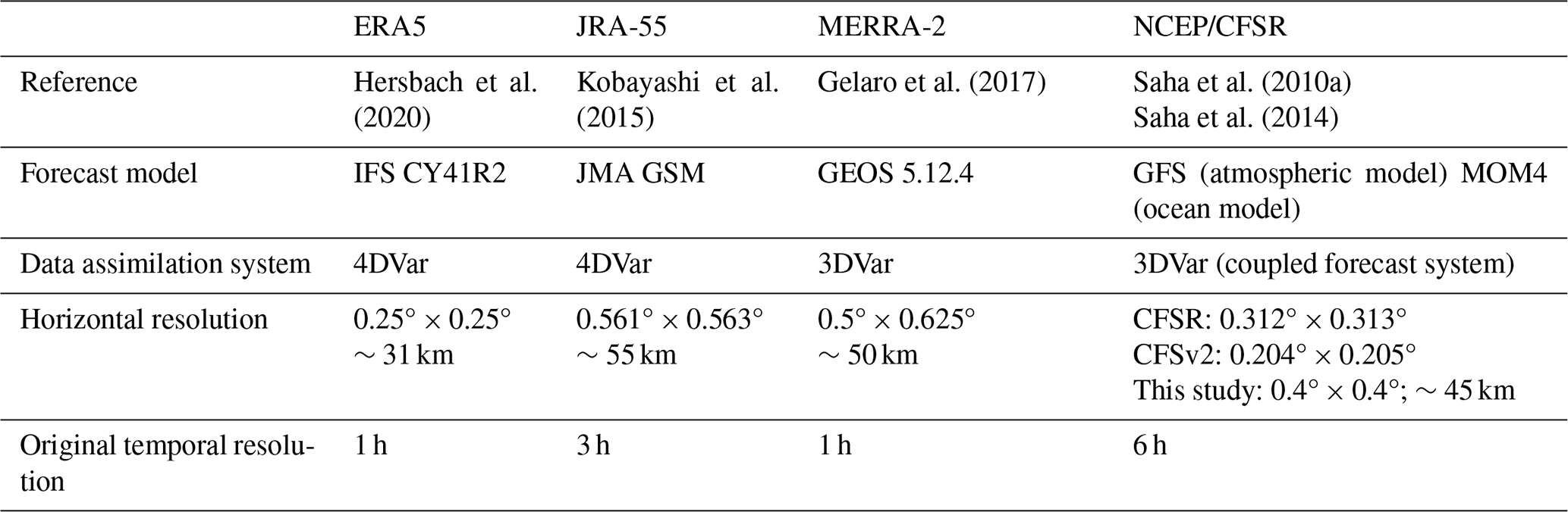
Table 2Representation of the sea ice in reanalyses.
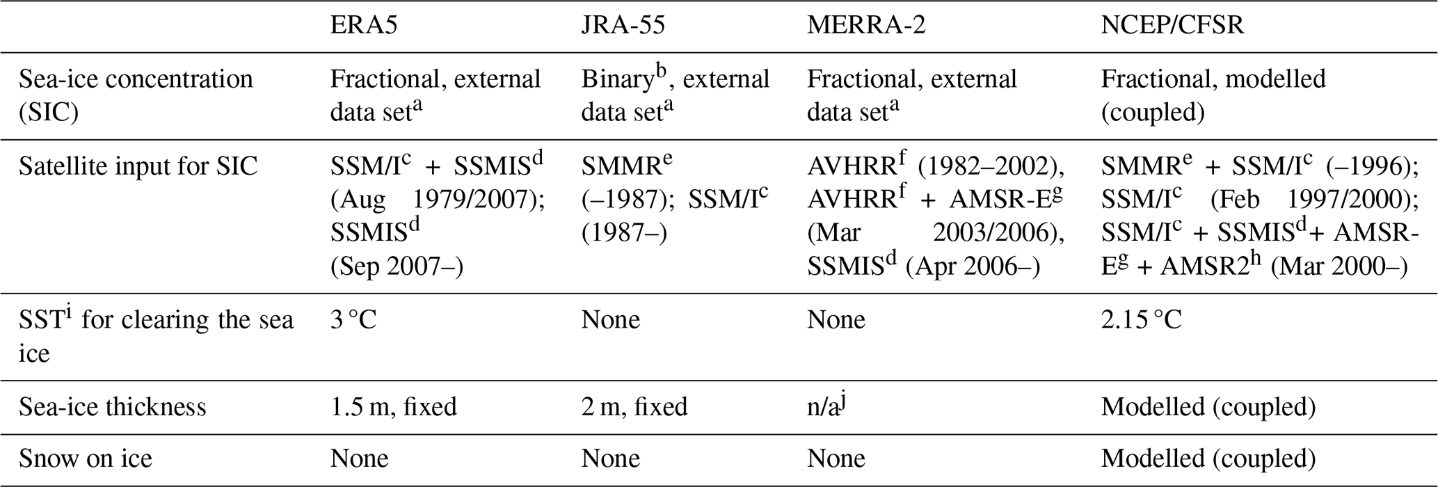
a See text for details. b SIC , SIC . c Special Sensor Microwave/Imager. d Special Sensor Microwave Imager-Sounder. e Scanning Multichannel Microwave Radiometer. f Advanced Very-High-Resolution Radiometer. g Advanced Microwave Scanning Radiometer – Earth Observing System sensor. h Advanced Microwave Scanning Radiometer 2. i Sea-surface temperature. j A 7 cm ice layer for computing a prognostic ice surface temperature, which is then relaxed towards 273.15 K as a representation of the upward oceanic heat flux. n/a: not applicable
From each reanalysis, we utilised the following variables: sea-ice concentration (SIC); surface latent heat flux (LHF); surface sensible heat flux (SHF); specific humidity at 2 m (Q2 m); temperature at 2 m (T2 m); temperature at the surface (Ts); and the U component (u) and V component (v) of the wind, both at 10 m. The signs of both turbulent heat fluxes were assigned with regard to the surface: a positive LHF referred to condensation and deposition and a negative LHF to evaporation and sublimation; a positive SHF referred to a downward flux and a negative SHF to an upward flux. Because Q2 m is not archived in ERA5 data sets, we followed Eqs. (7.4) and (7.5) from ECMWF (2016) to calculate it using the dew-point temperature and surface pressure. Subsequently, we obtained the temperature difference between 2 m height and the surface (Tdiff) by subtracting Ts from T2 m, and we calculated the wind speed (WS10 m) using u and v. To obtain the difference in specific humidity between the surface and 2 m height (Qdiff), we first computed the specific humidity at the surface (Qs) according to Iribarne and Godson (1973) using Ts. For the calculation of Qdiff, we then subtracted Qs from Q2 m, analogously to the Tdiff calculation.
Using data from each reanalysis, we studied the bilateral relationships of the turbulent heat fluxes LHF and SHF with SIC and the multilateral relationships between LHF (SHF), SIC, Qdiff (Tdiff), and WS10 m – the latter three variables being selected based on the LHF and SHF bulk parameterisation. In reanalyses, the general bulk parameterisation of surface turbulent fluxes is grid averaged taking into account different surface types with different surface temperatures (Claussen, 1991; Koster and Suarez, 1992). In our case, the different surfaces within a grid cell were sea ice and water, so the bulk formulae for the grid-averaged LHF (〈LHF〉) and SHF (〈SHF〉) include SIC, as shown in Vihma (1995):
where V stands for the wind speed at the lowest atmospheric level of the model applied in each reanalysis, ρ for the air density, LE for the latent heat of sublimation, and cp for the specific heat of the air, and the CHE parameters are the turbulent exchange coefficients; (Qa−Qs) and (θa−θs) are the differences in specific humidity and potential temperature between the lowest atmospheric level and the surface. In our study (specifically in Sect. 3.3), we apply the true Ts and T2 m when studying their effect on SHF because the adiabatic correction in a 2 m layer is negligible. The surface temperatures over the water and both snow-covered and bare sea ice are calculated from the surface energy budget in each reanalysis. The turbulent exchange coefficients (CHE) depend on the roughness lengths for momentum, heat, and moisture and on the stratification of the atmospheric surface layer.
For the bilateral relationship analysis, we utilised orthogonal-distance regression (ODR; Boggs et al., 1988). Because all variables in reanalyses include uncertainties, we theoretically considered ordinary-least-squares regression (OLSR), which assumes that there are no errors in the independent variable – not optimal for this case. Additionally, we carried out tests on bilateral ODR and OLSR performance using data from several grid cells from each reanalysis. While we found “nearly identical” (identical to at least five decimal places) coefficients of determination (the correlation coefficient squared, R2) for both regression methods, importantly, the slopes of the regression lines varied considerably. This is attributable to the above-mentioned OLSR's assumption of no errors in the independent variable (x; SIC in our case), so only the distance from the x data to the regression line is minimised, whereas ODR minimises the orthogonal distances of both the x and y data (in our case, y is LHF or SHF) from the regression line. Utilising the same above-described tests to compare the ODR performance with that of OLSR for multilateral regression analysis, however, we found that ODR and OLSR gave nearly identical values for the slopes of the regression lines between LHF (SHF) and SIC, Qdiff (Tdiff), and WS10 m. ODR and OLSR also gave nearly identical values of R2 for all and individual components of the multilateral regression. Based on the findings that both methods yielded nearly identical results for the multilateral regression analysis (using our reanalysis data), we decided to use OLSR for the multilateral regression analysis in our work, as it requires far fewer computing resources to perform. We used a linear model for both ODR and OLSR, as we evaluated that it was the most applicable for our purposes, although we were aware of some non-linearity in the effect of SIC on Q2 m (T2 m) and LHF (SHF), as shown for near-surface air temperature in, for example, Fig. 4 of Lüpkes et al. (2008).
The statistical significance testing of the results (the slopes for LHF and SHF and their explanatory variables) was performed using Student's t test (95 % confidence interval) with adjusted degrees of freedom (DFadj) according to Eq. (31) from Bretherton et al. (1999):
where T stands for the number of days in one sample (in our case the days in seasons during the periods of 1980–2000 and 2001–2021), and R1 and R2 stand for the correlation coefficient for the lag 1 autocorrelation of the turbulent heat flux (LHF or SHF) and its explanatory variable (SIC), respectively.
Each reanalysis typically uses not only its own (1) data-assimilation system, (2) forecast model (as seen in Table 1), and often (3) different parameterisation schemes for subgrid-scale variables (such as turbulent fluxes), but also more or less (4) different atmospheric and surface observations and (5) different representations of the sea ice. In Table 2, we describe the representation of sea ice in selected reanalyses, which can have a considerable effect on the modelling of the lower troposphere. The external data sets (unspecified in Table 2) used as sources for SIC in ERA5, JRA-55, and MERRA-2 are as follows. ERA5 uses data from OSI SAF (Ocean and Sea Ice Satellite Application Facility) of EUMETSAT (European Organisation for the Exploitation of Meteorological Satellites), version OSI SAF (409a), for January 1979 through August 2007, and it uses OSI SAF oper for September 2007 onwards (Hersbach et al., 2020). In JRA-55, daily data on the conditions for SIC are obtained from COBE-SST (Centennial In Situ Observation-based Estimates of the Variability of Sea Surface Temperatures and Marine Meteorological Variables) (Kobayashi et al., 2015; Matsumoto et al., 2006). MERRA-2 uses monthly data from CMIP (Coupled Model Intercomparison Project), as in Taylor et al. (2000), prior to 1982; data from OISST (Optimum Interpolation Sea Surface Temperature) from NOAA (National Oceanic and Atmospheric Administration) for 1982 to March 2006; and data from OSTIA (Operational Sea Surface Temperature and Ice Analysis) from the Met Office from April 2006 onwards (Gelaro et al., 2017).
3.1 Differences in sea-ice concentration and surface turbulent fluxes
To illustrate the climatology in and differences in sea-ice concentration (SIC), latent heat flux (LHF), and sensible heat flux (SHF) between the four selected reanalyses, we calculated the mean biases of daily field means (hereafter referred to as “mean biases”) between NCEP/CFSR and other reanalyses (ERA5, JRA-55, MERRA-2) in nine Arctic basins (Fig. 1) in all seasons and the two study periods (Figs. 2, 3, and S2). NCEP/CFSR appears to be the most realistic in terms of physical processes due to its modelled sea-ice thickness and the snow on top of sea ice (see more in Sect. 3.4); however, we do not assume that it is the best reanalysis with respect to turbulent surface fluxes, and we use mean biases to present an overview and comparison of the typical values in all reanalyses. Mean values (temporal together with spatial) of NCEP/CFSR variables in Arctic basins, seasons, and periods are shown in Tables 3, 4, and S1. The mean values of NCEP/CFSR variables in these tables are not directly comparable with the values of mean biases of daily field means between NCEP/CFSR and other reanalyses presented in Figs. 2, 3, and S2, as the methods used to calculate them are different. However, we can obtain estimates of the absolute values of SIC, LHF, and SHF in ERA5, JRA-55, and MERRA-2 by looking at Tables 3, 4, and S1 together with Figs. 2, 3, and S2. For the calculations of both mean biases and mean values, we used land–sea masks provided by each reanalysis and only considered grid cells completely covered by the sea.
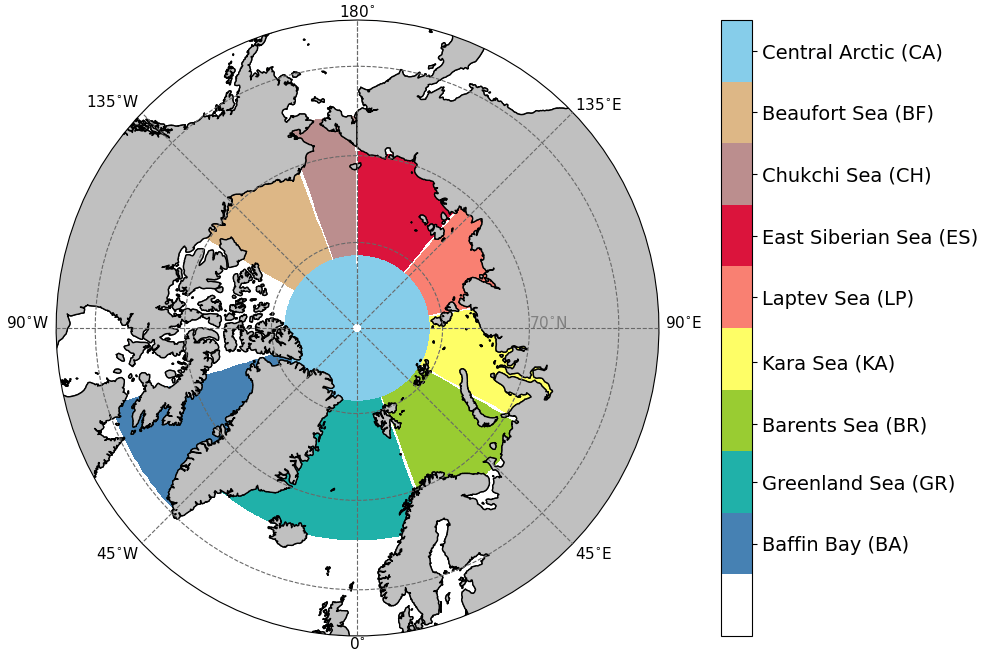
Table 3Mean sea-ice concentration in Arctic basins as represented in NCEP/CFSR in November–December–January (NDJ), February–March–April (FMA), May–June–July (MJJ), and August–September–October (ASO) during the time periods 1980–2000 (I) and 2001–2021 (II).
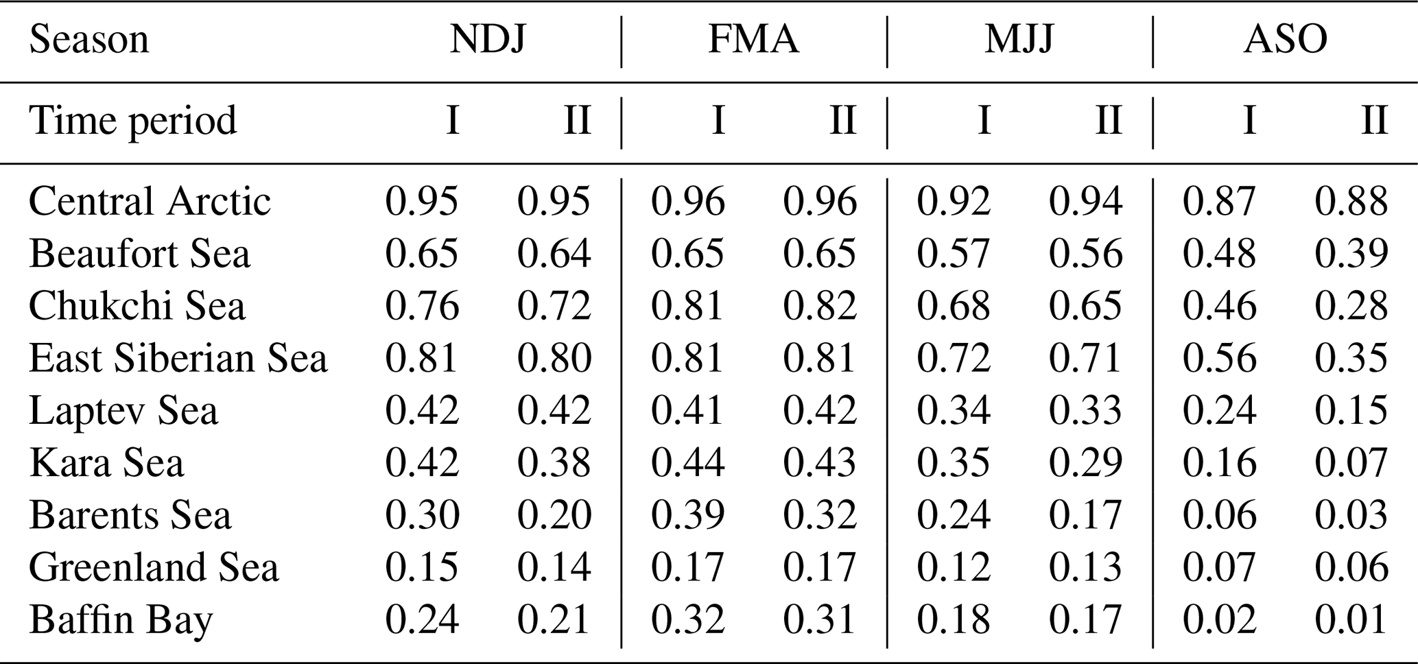
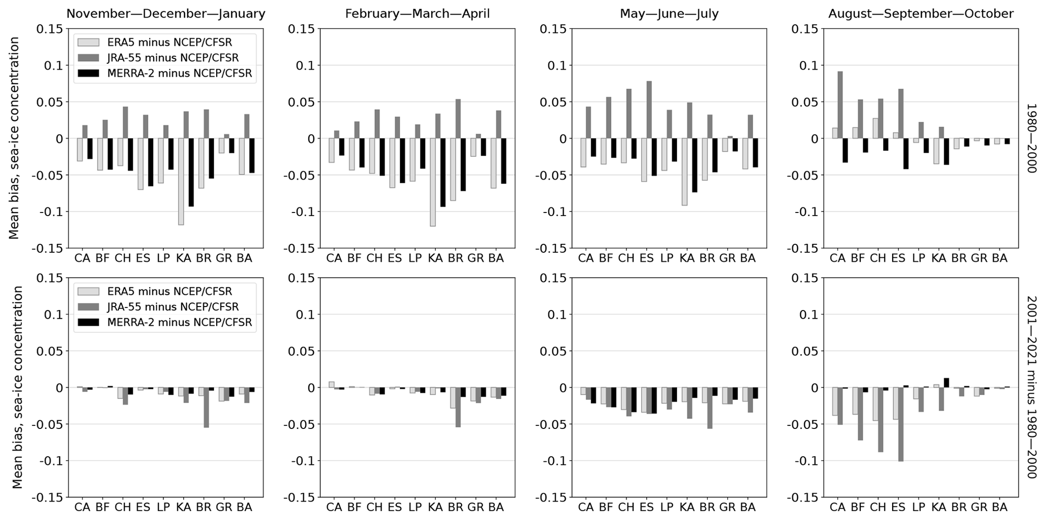
Figure 2Mean biases of daily field means of sea-ice concentration: ERA5 minus NCEP/CFSR (light grey), JRA-55 minus NCEP/CFSR (grey), and MERRA-2 minus NCEP/CFSR (black). The horizontal axis refers to the Arctic basins shown in Fig. 1. The first row shows data from the period 1980–2000, and the second row shows the difference between the period 2001–2021 and the earlier period. Only grid cells fully covered by sea were considered in this analysis.
Table 4Mean latent heat flux (W m−2) in Arctic basins as parameterised in NCEP/CFSR in November–December–January (NDJ), February–March–April (FMA), May–June–July (MJJ), and August–September–October (ASO) during the time periods 1980–2000 (I) and 2001–2021 (II).
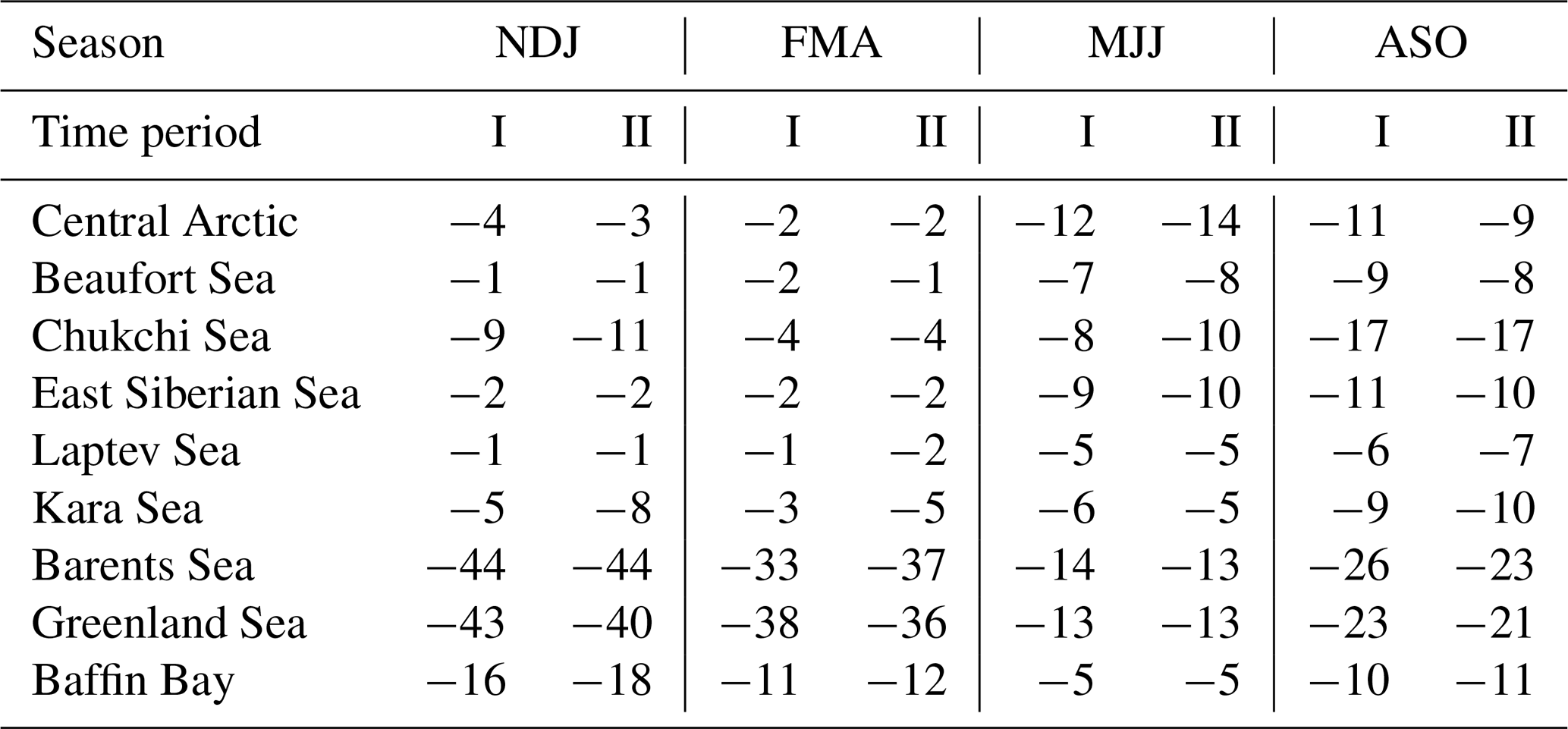
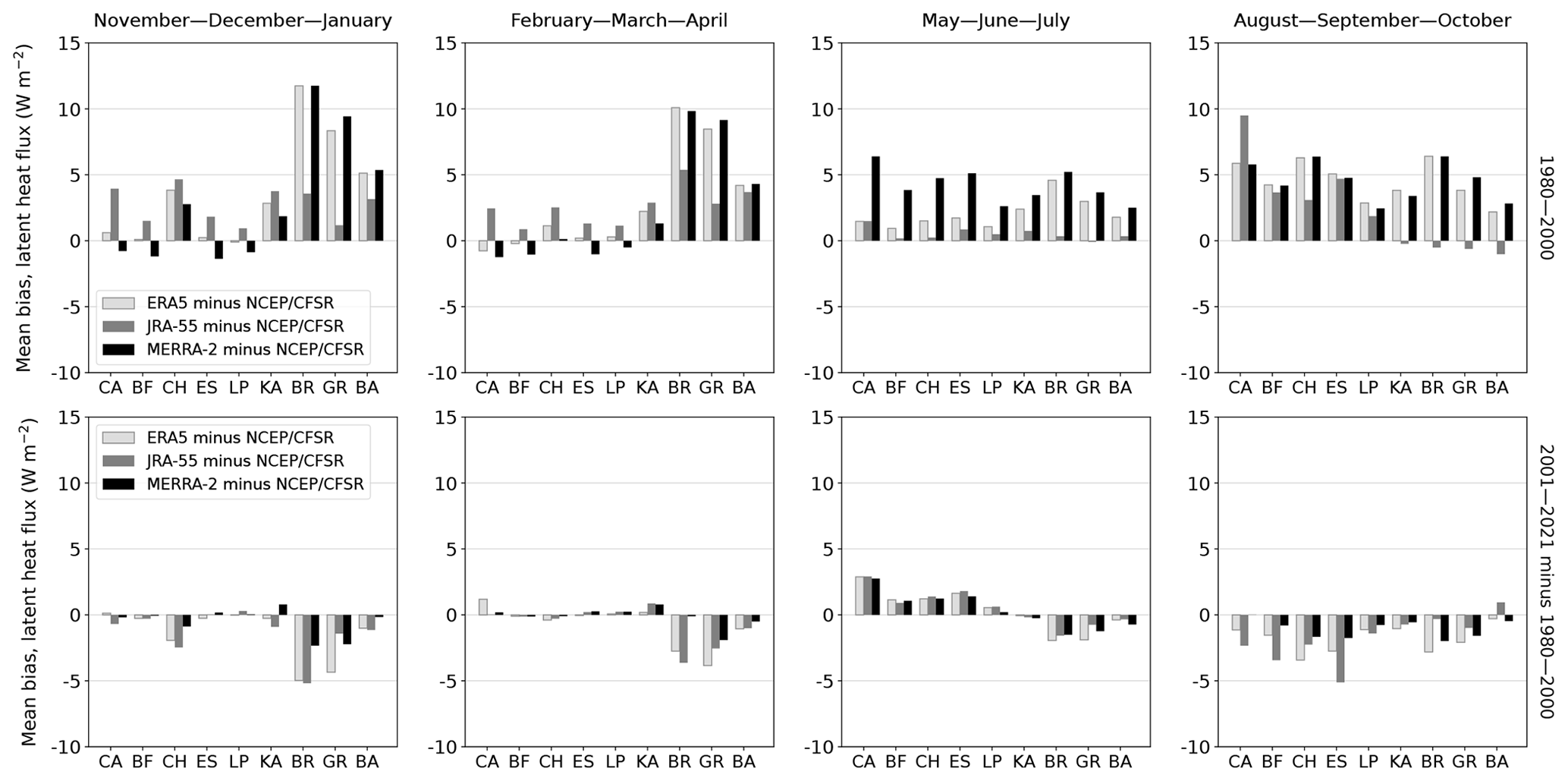
Figure 3Mean biases of daily field means of latent heat flux: ERA5 minus NCEP/CFSR (light grey), JRA-55 minus NCEP/CFSR (grey), and MERRA-2 minus NCEP/CFSR (black). The horizontal axis refers to the Arctic basins shown in Fig. 1. The first row shows data from the period 1980–2000, and the second row shows the difference between the period 2001–2021 and the earlier period. Only grid cells fully covered by sea were considered in this analysis.
The mean SIC in NCEP/CFSR ranged from 0.01 in Baffin Bay in August–September–October in 2001–2021 to 0.96 in the Central Arctic in February–March–April in both 1980–2000 and 2001–2021 (Table 3). The value of the mean SIC decreased in nearly all basins between the periods 1980–2000 and 2001–2021: by 2 % to 33 % in November–December–January, 2 % to 18 % in February–March–April, 1 % to 29 % in May–June–July, and 14 % to 56 % in August–September–October. On the contrary, it increased by up to 2 % or remained the same between the two study periods in the Central Arctic in all seasons and in several other basins in February–March–April.
The mean biases between NCEP/CFSR and other reanalyses in SIC (calculated as a reanalysis minus NCEP/CFSR; Fig. 2) were between −0.1 and +0.05 SIC in nearly all regions and seasons in 1980–2000, with mostly negative mean biases between NCEP/CFSR and ERA5 and between NCEP/CFSR and MERRA-2 and mostly positive mean biases between NCEP/CFSR and JRA-55. For most of the data in 1980–2000, the differences between ERA5 and JRA-55 were the largest, up to 0.15 in the Kara Sea in November–April, while the differences between ERA5 and MERRA-2 were the lowest. In the cold season (November–April), JRA-55 had a lower magnitude of mean bias in SIC with respect to NCEP/CFSR than ERA5 and MERRA-2 did in most cases. This is an interesting result because JRA-55 has a binary representation of SIC (assigning a value of 1 for a SIC of over 0.55 in a grid cell and a value of 0 for a SIC equal to or less than 0.55), whereas nearly all concentrations are considered in the other reanalyses (SIC range from 0 to 1 in MERRA-2 and from 0.15 to 1 in ERA5 and NCEP/CFSR). The magnitude of mean bias between NCEP/CFSR and JRA-55 mostly decreased in 2001–2021, while that between NCEP/CFSR and ERA5 and that between NCEP/CFSR and MERRA-2 increased in many basins, especially in May–June–July.
We found the mean LHF in NCEP/CFSR to be negative in all basins and seasons and in both periods (Table 4). The smallest magnitude of the mean flux occurred in the Laptev and Beaufort seas (−1 W m−2) and the largest occurred in the Barents Sea (−44 W m−2), with both occurring in November–December–January. Corresponding to the changes in mean SIC between the two study periods, in the cold season (November–April), the mean negative LHF intensified in the majority of the basins with decreased SIC. Values of mean bias in LHF between NCEP/CFSR and other reanalyses were mostly between −5 and +10 W m−2 (Fig. 3). As in the case of the SIC, mean biases between NCEP/CFSR and ERA5 and between NCEP/CFSR and MERRA-2 were the highest and differences between ERA5 and MERRA-2 were the lowest for most basins and seasons. The most noticeable results in the period 1980–2000 were large positive mean biases during November–April in the Barents and Greenland seas between NCEP/CFSR and ERA5 and between NCEP/CFSR and MERRA-2. These findings were not consistent with the theoretical expectations – negative mean biases in SIC being followed by negative mean biases in LHF (less sea ice resulting in more evaporation/sublimation than in NCEP/CFSR). However, as we will show in Sect. 3.2 (Figs. 4 and S4), in November–April, the correlations between SIC and LHF in ERA5 and MERRA-2 are not different in sign from those in NCEP/CFSR and do follow the theoretical expectations for this relationship. Because the sea ice covers only a small part of the Greenland and Barents sea basins (even in November–April), and we calculated the mean surface turbulent fluxes and mean biases using the whole extent of each basin (as shown in Fig. 1), the smaller magnitude of the negative LHF in ERA5 and MERRA-2 compared to NCEP/CFSR is likely due to the differences in other factors affecting LHF (see Eq. 1) in the ice-free areas of these basins. As for the mean biases in LHF between NCEP/CFSR and ERA5, JRA-55, or MERRA-2, their magnitudes mostly decreased in nearly all basins and seasons in 2001–2021 compared to 1980–2000.
The mean SHF in NCEP/CFSR ranged from 0 W m−2 in the Kara Sea in February–March–April 2001–2021 to −49 W m−2 in the Barents Sea in November–December–January 1980–2000 (Table S1). Mean biases in SHF between NCEP/CFSR and other reanalyses (Fig. S2) ranged mostly between +10 and −20 W m−2 in November–April and between +5 and −10 W m−2 in May–October. We found that the largest magnitude of mean bias occurred between NCEP/CFSR and ERA5 and between NCEP/CFSR and MERRA-2 in November–April (over −20 W m−2 for MERRA-2 data in the Central Arctic in November–December–January). As in the case of the LHF, in the Atlantic sector of the Arctic Ocean in November–April, negative mean biases in SIC (Fig. 2) were accompanied by positive mean biases in SHF (Fig. S2). The explanation for this seemingly non-physical relationship is the same as that given in the previous paragraph. Additionally, we show in Sect. 3.2 (Figs. 6 and S7) that the SIC/SHF correlation in November–April is the same sign in all four reanalyses in our study. Similarly to the mean biases in LHF, the magnitude of differences between reanalyses decreased to some extent in most basins in 2001–2021 compared to 1980–2000.
3.2 Effect of sea-ice concentration on surface turbulent fluxes
To investigate the relationships between Arctic SIC and surface turbulent fluxes in reanalysis data, we first carried out bilateral orthogonal-distance regression (ODR) analyses between SIC and LHF and between SIC and SHF. For these analyses, we only included data (grid cells) with a mean SIC of >0.5 in each period and season.
In Fig. 4, we illustrate the change in LHF (W m−2) per unit of SIC (slope of the regression line) in November–December–January in the periods 1980–2000 and 2001–2021, and we show the difference between 2001–2021 and 1980–2000. The correlation between SIC and LHF in the Arctic in these months was solely positive (shades of red in Fig. 4a–h), meaning less sea ice–more evaporation/sublimation. This finding was consistent with the theoretical expectation that large amounts of moisture are released into the dry winter Arctic air from the (relatively) warm ocean when it is exposed by the retreat of sea ice. Although the direction of the relationship was the same in all four reanalyses, there were differences in its strength. While we found the slopes of the regression lines between SIC and LHF to be around 200–300 W m−2 LHF per unit of SIC (change in SIC from 0 to 1) in ERA5, JRA-55, and MERRA-2, we observed values of up to 600 W m−2 LHF per unit of SIC in the NCEP/CFSR data, indicating a much higher sensitivity of LHF to SIC in the marine Arctic in this reanalysis (further addressed and explained in Sect. 3.4). The large dark grey areas in the JRA-55 results (Fig. 4b, f, j) indicate failures of the linear bilateral ODR model due to the binary representation of SIC in this reanalysis. Because the SIC in these dark grey areas was never less than 0.55 during the 21-year periods, every grid cell was assigned a value of 1, making it impossible for the model to explain the variations in LHF by variations in SIC. Analogously, the dark grey areas appear in other reanalyses as well, due to very low SIC variability in some regions (which is further addressed and explained later in this subsection and in Figs. 6 and 7).
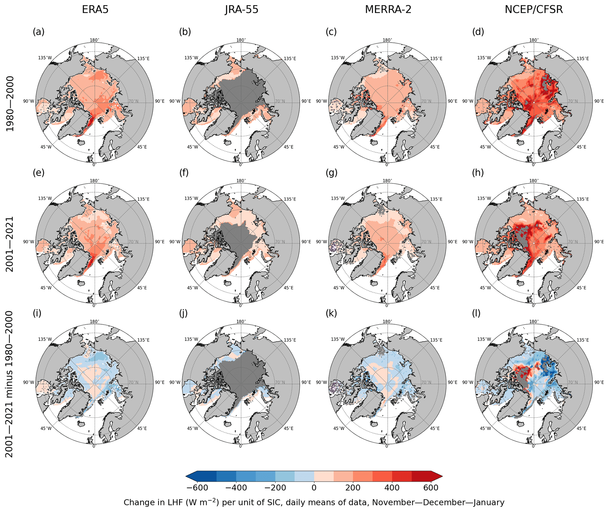
Figure 4Change in latent heat flux (W m−2) per unit of change in sea-ice concentration (slope of the regression line) in the marine Arctic in November–December–January in four reanalyses (columns), based on the linear orthogonal-distance regression (ODR) model. Panels (a)–(d) depict the period 1980–2000, panels (e)–(h) show the period 2001–2021, and panels (i)–(l) show the difference between 2001–2021 and 1980–2000. Dark grey indicates areas where the ODR model did not converge; in (i)–(l), dark grey indicates areas that did not converge for 1980–2000 and/or 2001–2021. Only grid cells with a mean SIC of >0.5 were considered, and only statistically significant results within the 95 % confidence interval are shown.
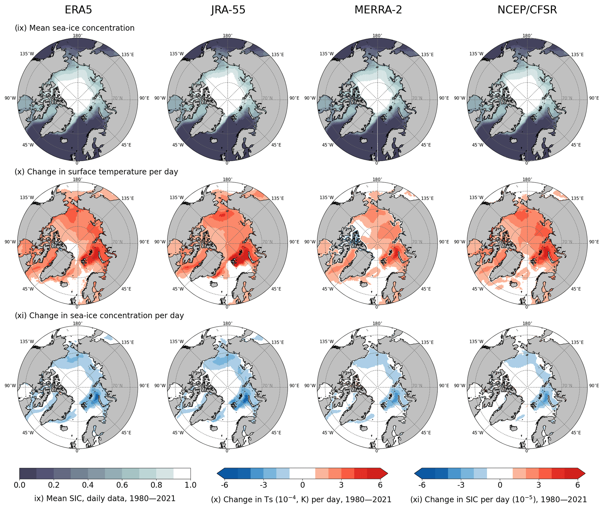
Figure 5Mean sea-ice concentration (row ix), change in surface temperature per day (row x), and change in sea-ice concentration per day (row xi) during 1980–2021; daily means of data in four reanalyses are shown. Changes in the variables per day are the slopes of the ordinary-least-squares regression lines using time as an independent variable.
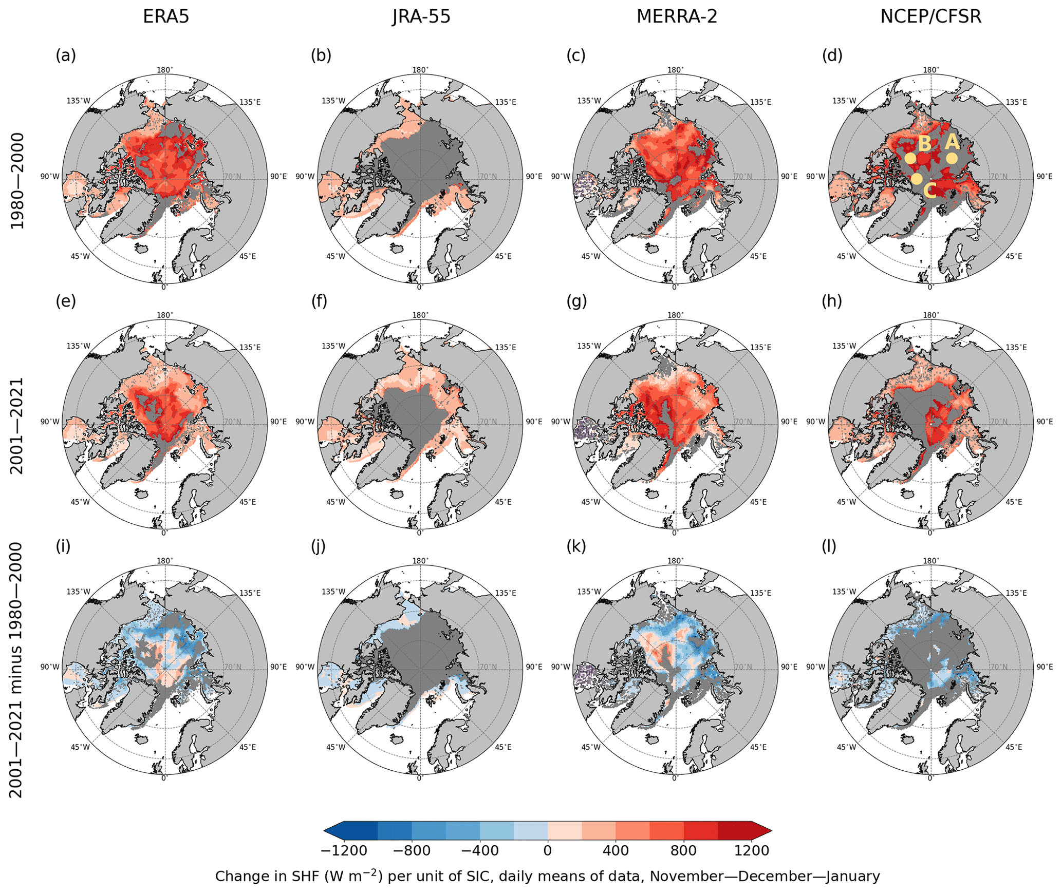
Figure 6Change in sensible heat flux (W m−2) per unit of change in sea-ice concentration (slope of the regression line) in the marine Arctic in November–December–January as represented in four reanalyses (columns), based on the linear orthogonal-distance regression (ODR) model. Panels (a)–(d) depict the period 1980–2000, panels (e)–(h) show the period 2001–2021, and panels (i)–(l) show the difference between 2001–2021 and 1980–2000. Dark grey indicates areas where the ODR model did not converge; in (i)–(l), dark grey indicates areas that did not converge for 1980–2000 and/or 2001–2021. Points A, B, and C in (d) are further analysed in Fig. 7. Only grid cells with a mean SIC of > 0.5 were considered, and only statistically significant results within the 95 % confidence interval are shown.
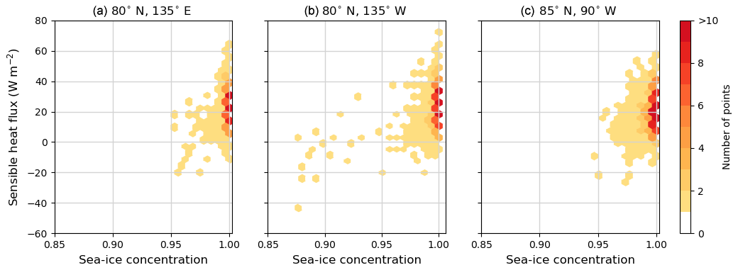
Figure 7Daily sea-ice concentration and sensible heat flux in three selected grid cells from dark grey areas indicated in Fig. 6; NCEP/CFSR data, days in November–December–January in 1980–2000 (1932 d). (a) Grid cell A nearest to 80° N, 135° E; (b) grid cell B nearest to 80° N, 135° W; (c) grid cell C nearest to 85° N, 90° W.
A positive correlation between SIC and LHF could also be observed in February–March–April and August–September–October (shades of red in Figs. S4 and S6a–h), with a generally stronger relationship between the variables than in November–December–January. In May–June–July, however, the relationship between SIC and LHF turned into a negative correlation in most areas, meaning less sea ice–less evaporation (shades of blue in Fig. S5a–h). In this season, we found the strongest SIC/LHF relationship in the Central Arctic (north of 81.5° N) for all reanalyses, ranging from around 300 W m−2 in MERRA-2 to 400–600 W m−2 in ERA5 and NCEP/CFSR. The negative correlation between SIC and LHF in May–June–July can be explained as follows. Based on various SIC thresholds, the reanalyses keep the sea-surface temperature relaxed to the seawater freezing point (approximately −1.8 °C) throughout the year (e.g. in Ishii et al., 2005; Good et al., 2020), often resulting in the open water being colder than melting snow/ice in summer, when the surface temperature is 0 °C (Persson et al., 2002; Vihma et al., 2008; Walden et al., 2017). Accordingly, the surface temperatures favour less evaporation over the open water than over melting sea ice.
The effect of SIC on LHF in all seasons (as parameterised in reanalyses) weakened between the two periods for most of the Arctic (shades of blue in Figs. 4, S4, S6i–l; shades of red in Fig. S5i–l). To interpret this change, we produced Fig. 5, which shows that the surface temperature (Ts) rose nearly everywhere in the marine Arctic between 1980–2021 (row x). The strongest surface warming in the Barents, Kara, Laptev, and Chukchi seas can be attributed to the sea ice being replaced by the warmer sea to a large extent (see the areas of strongest sea-ice decline in row xi). The warming in other areas (including the Central Arctic, where the mean SIC in 1980–2021 was 0.9–1; see row ix) indicates a warming of the sea-ice surface in past decades. Based on these findings, we present the following explanations of why the SIC/LHF relationship weakened between the two study periods. (1) For leads opening in otherwise mostly compact sea ice, the surface temperature of the sea ice has increased while the underlying sea temperature has remained the same (at the seawater freezing temperature of approximately −1.8 °C); hence, the difference in surface saturation specific humidity between the sea ice and open water has decreased, directly contributing to a decreased sensitivity of LHF to SIC. (2) The sea ice has declined considerably or disappeared completely from some of the grid cells, so there is a very small to no effect of SIC on LHF in the latter study period. Mostly in the Central Arctic, however, we found some areas of increased SIC effect on LHF between 1980–2000 and 2001–2021 (shades of red in Figs. 4, S4, S6i–l; shades of blue in Fig. S5i–l, meaning a stronger relationship in 2001–2021). This increased SIC effect on LHF may be explained as follows. As mentioned before, the effect of SIC on the near-surface air temperature (and specific humidity) is not linear, but it is usually the strongest when leads open in areas where the SIC is very close to 1. As indicated in Table 3 and shown in our representative grid cells (Fig. S3), SIC increased in some areas of the Central Arctic between 1980–2000 and 2001–2021 (possible reasons for this are discussed in Sect. 4.5). Therefore, SIC was mostly very high in 2001–2021, meaning that even a very small decrease in SIC has a strong effect on near-surface air temperature and specific humidity. We cannot be sure, however, whether SIC increased in reality in these parts of the Central Arctic in 2001–2021 compared to 1980–2000; we only comment on possible physical and statistical explanations of the phenomena presented in the reanalysis data.
Also for SHF, the change in the flux per unit of SIC (the slope of the regression line) depended on the season, region, and decadal period (Figs. 6, S7–S9). As in the case of the SIC/LHF relationship, SIC and SHF were positively correlated in the Arctic in November–December–January (shades of red in Fig. 6a–h), meaning less sea ice–more upward (negative) SHF. These results are also consistent with the theoretical expectations as mentioned above: the sea is considerably warmer than the near-surface air in the cold season (November–April), and when the insulating sea-ice layer retreats, a large amount of upward SHF is released. The strength of the SIC/SHF correlation ranged from around 300 W m−2 SHF per unit of SIC in the JRA-55 data (keeping in mind the limited area in which it was possible to analyse the relationship) to around 800 W m−2 SHF per unit of SIC in ERA5, NCEP/CFSR, and MERRA-2. Similarly to SIC/LHF, there were dark grey areas (grid cells) where the linear bilateral ODR model did not converge in our SIC/SHF regression analysis results. As we mentioned above, in the case of JRA-55 (Fig. 6b, f, j), the failure of the model was caused by the binary representation of SIC in this reanalysis, which makes it impossible for the model to explain the variations in LHF or SHF by the variations in SIC. In Fig. 7, using grid cells from dark grey areas from NCEP/CFSR data, we show that in cold seasons, the reason for the failure of the model is similar in reanalyses with a fractional representation of SIC – very low SIC variability and high SHF variability. In these selected grid cells, the SIC mostly varied only between 0.95 and 1, while SHF showed variability between −20 and 60 W m−2. On most days (the highest density of points, darkest orange/red), the SIC was 1 and SHF was 0–30 W m−2, resulting in no clear bilateral relationship.
As with the SIC/LHF relationship, we also found a positive SIC/SHF correlation in February–March–April and partly so in August–September–October (shades of red in Figs. S7 and S9a–h). The areas where the linear ODR model did not converge expanded considerably in February–March–April compared to November–December–January, probably due to less variation in SIC during February–March–April (before the melting starts) compared to November–December–January (with the sea typically just starting to freeze in November). The fact that there are more dark grey areas in Figs. 6 and S7 (SIC/SHF relationship, November–April) than in Figs. 4 and S4 (SIC/LHF relationship, November–April) can be attributed to greater variability in SHF than in LHF in the Arctic during these seasons, making it harder for the model to fit a regression line when SIC is very high. In May–June–July, the SIC/SHF relationship also turned into a negative correlation (shades of blue in Fig. S8), meaning less SIC–more downward (positive) SHF. We observed a similar spatial distribution of the correlation strength to that seen in the SIC/LHF results for May–June–July, with the maximum slope of the regression line occurring in the Central Arctic (around 400 W m−2 per unit of SIC in ERA5 and MERRA-2 and up to 800 W m−2 per unit of SIC in NCEP/CFSR). The summer change in the slope sign can be explained analogously to the SIC/LHF relationship: the open water at the seawater freezing point (−1.8 °C) is colder than the summer-ice surface temperature at about the snow/ice melting point (0 °C). Therefore, opening leads (i.e. reducing the sea ice) induces more downward (positive) SHF in reanalyses.
The SIC effect on SHF weakened between 1980–2000 and 2001–2021 in most of the Arctic and strengthened in some parts of the Central Arctic and Beaufort Sea across all the seasons (shades of blue in Figs. 6, S7, S9i–l; shades of red in Fig. S8i–l) very similarly to the SIC/LHF relationship. The same explanation for this trend is valid for the change in SIC/SHF relationship: the increasing surface temperature of the sea ice reduces the surface temperature difference between ice and water, directly contributing to the lower sensitivity of SHF to SIC. The stronger relationship between SIC and SHF in the Central Arctic and Beaufort Sea in 2001–2021 compared to 1980–2000 (shades of red in Figs. 6, S7, S9i–l; shades of blue in Fig. S8i–l) can be explained in similar terms to the increased SIC effect on LHF described earlier in this subsection.
3.3 Multiple drivers of surface turbulent fluxes
To assess more drivers of the surface turbulent fluxes in reanalyses (as shown in the fluxes' bulk parameterisation in Eqs. 1 and 2), we further performed linear multilateral ordinary-least-squares regression (OLSR) analyses utilising SIC, the specific-humidity difference (Qdiff, Q2 m minus Qs), and wind speed at 10 m (WS10 m) as explanatory variables for the variance in LHF and utilising SIC, the temperature difference (Tdiff, T2 m minus Ts), and wind speed at 10m (WS10 m) as explanatory variables for SHF variance. As an outcome of these analyses, we studied the variances in LHF and SHF (vLHF and vSHF, respectively) that were explained by the model (coefficient of determination, R2) overall and the proportion of the overall R2 explained by each of the three drivers mentioned above.
Besides the decline in the sea-ice extent, we found both the overall and partial values of R2 in 1980–2000 to be quantitatively very similar to those in 2001–2021 in all reanalyses and seasons and for both LHF and SHF (Figs. 8, S10–S24).
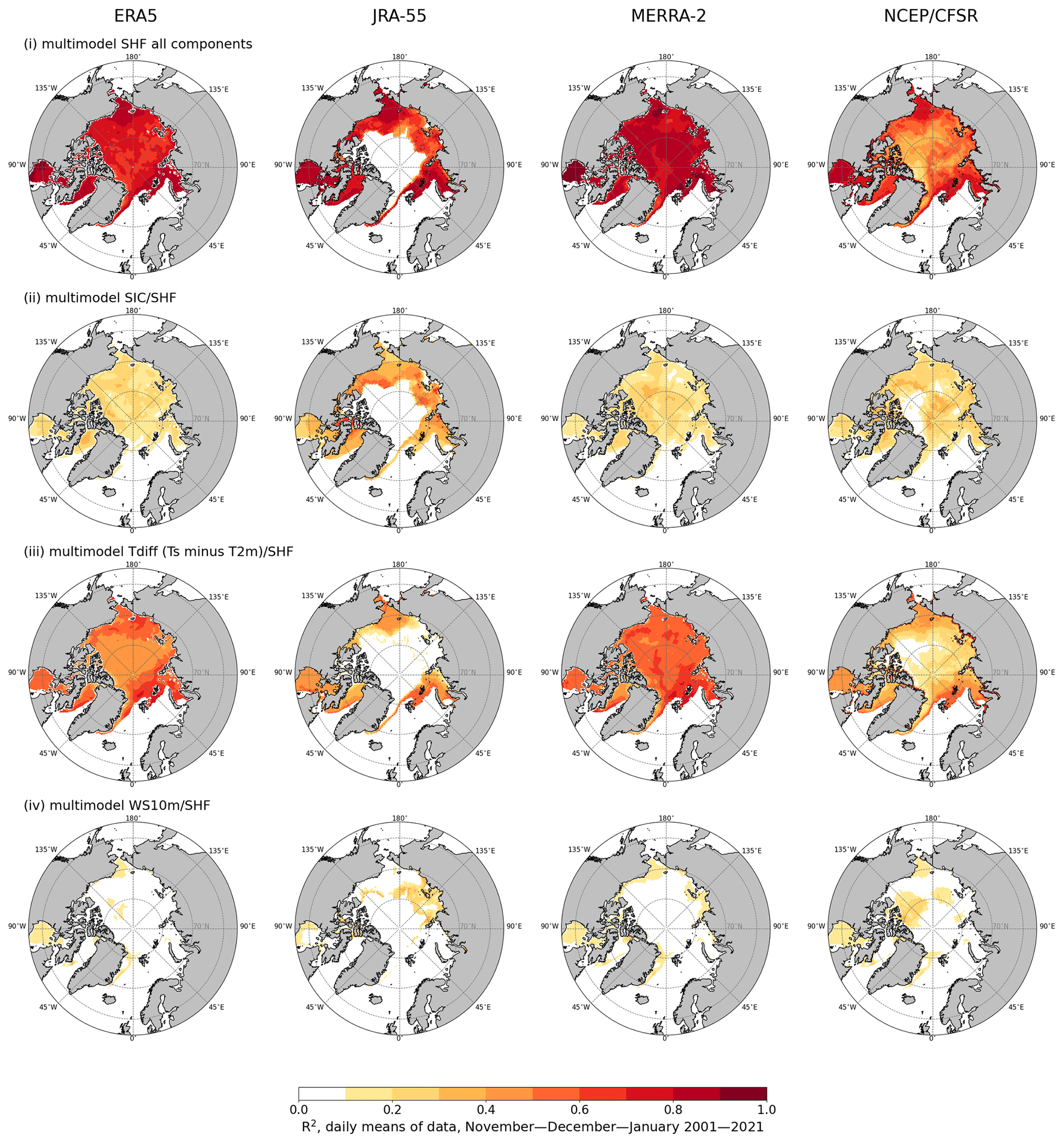
Figure 8Proportion of variance in the sensible heat flux (vSHF) explained by the linear ordinary-least-squares regression model (coefficient of determination, R2); daily means of data, November–December–January, 2001–2021. Row (i) shows the vSHF explained by all components: the SIC/temperature difference (T2 m minus Ts, Tdiff)/wind speed (10 m, WS10 m); row (ii) shows the vSHF explained by the SIC/SHF component of the model; row (iii) shows the vSHF explained by the Tdiff/SHF component of the model; and row (iv) shows the vSHF explained by the WS10 m/SHF component of the model. Only grid cells with a mean SIC of > 0.5 were considered.
During the cold season (November–April), the model explained around 80 % of vSHF, with similar spatial distributions seen for ERA5, JRA-55, and MERRA-2 (Figs. 8, S10–S12). The partial R2 also had similar values for these three reanalyses – around 20 % of vSHF was explained by SIC, around 50 % was explained by Tdiff, and around 10 % was explained by WS10 m. In NCEP/CFSR in November–April, however, the model explained only around 40 %–50 % of vSHF nearly everywhere outside of the marginal-ice zone. In these regions, while the partial R2 explained by SIC and WS10 m had about the same values as in the remaining three reanalyses, the partial R2 for Tdiff only reached values of around 20 %–30 %. During the warm season (May–October; Figs. S13–S16), however, both the overall and partial R2 in NCEP/CFSR were about the same as those in the other reanalyses (about 70 %–80 % overall: around 10 % for SIC, 60 % for Tdiff, and mostly <10 % for WS10 m). Hence, the cold-season difference in NCEP/CFSR results is likely due to the role of snow on the sea ice (which is present and modelled in this reanalysis, unlike the other ones). Insulation by snow causes a lower Ts because it reduces the upward conductive heat flux from the ocean under the sea ice to the snow surface. A lower Ts reduces Tdiff in the very cold November–April conditions in the Arctic. At the same time, when a lead opens, the difference between Ts of the snow and Ts of the water is much larger than the difference between the Ts values of bare sea ice and water, resulting in a larger magnitude of upward SHF than in the case of a bare sea-ice surface compared to open water. In November–April, this should make the variance in SIC more important for explaining vSHF, accounting for the lower importance of Tdiff in NCEP/CFSR than in the remaining reanalyses. However, according to our results in Figs. 8 and S10–S12, this was mostly not the case. As we present for bilateral relationships between SIC and SHF in Figs. 6 and S7, the linear ODR model using NCEP/CFSR data did not converge in large areas of the marine Arctic in November–December–January, and in even larger areas in February–March–April, presumably due to very low variability in SIC and large variability in SHF, which points to the difficulty faced when using this kind of model to reproduce cold-season surface and near-surface-air conditions using NCEP/CFSR data.
The vLHF explained by the linear multilateral OLSR in the warm season (May–October; Figs. S21–S24) was very similar to that for vSHF for both study periods and all reanalyses – around 80 % overall (around 10 %–20 % for SIC, 50 %–60 % for Qdiff, and around 10 % for WS10 m). In November–April (Figs. S17–S20) in the NCEP/CFSR results, we also came across lower overall (and Qdiff) R2 values – around 40 % (and <10 %) in the areas where the SIC/LHF linear model failed. In other reanalyses in November–April, the overall vLHF explained by the model had about the same values as in the case of vSHF, although the partial R2 values for SIC were higher (around 40 % in November–December–January and around 30 % in February–March–April) and the partial R2 values for Qdiff were accordingly lower. Variations in WS10 m explained, on average, more vLHF than vSHF – around 10 %–20 %.
3.4 Thin ice on leads and snowpack on top of sea ice
In addition to the effects of SIC on turbulent fluxes, there are two factors that deserve particular attention: the effects of thin ice on leads and the effects of snowpack on top of sea ice.
Considering the first one, reanalyses assume that the open parts of each grid cell have a surface temperature at the freezing point of ocean water, −1.8 °C. However, in reality, winter leads typically remain open for less than a day (Makshtas, 1991) or just a few hours (Petrich et al., 2007) and are thereafter covered by thin ice with a surface temperature lower than −1.8 °C. This results in the overestimation of upward turbulent fluxes arising from leads in reanalyses. To estimate the magnitude of the overestimation, we carried out analytical calculations. We focused on the cold season when the insulating effect of the ice layer is largest so that the results represent the maximum effect of thin ice on leads. As a first approximation, we assume that the temperature profile through a thin ice layer is linear. Then the conductive heat flux C is
where ki stands for the heat conductivity of ice, Ts for the ice surface temperature, Tb for the ice bottom temperature (−1.8 °C), and hi for the ice thickness. The turbulent fluxes of sensible and latent heat were calculated by applying the standard bulk formulae (analogous to Eqs. 1 and 2 but for local instead of grid-averaged fluxes):
The upward long-wave radiation (ULW) was calculated as
where σ stands for the Stefan–Boltzmann constant ( ). The downward long-wave radiation (DLW) and the input for Eqs. (4)–(7) were taken from observations made in the Central Arctic during the SHEBA campaign (Persson et al., 2002) in February, when the mean values were as follows: 155 W m−2 for DLW, 5.0 m s−1 for V, −32 °C for Ta, and 0.9 for the relative humidity, yielding 0.17 g kg−1 for Qa and 2.1 W m−1 K−1 for ki. The LHF and SHF were first calculated for open leads using Eqs. (5) and (6) with Ts set to −1.8 °C. Then the calculations were repeated assuming different values for hi: 0.05, 0.1, and 0.15 m. As Ts is unknown and all the fluxes except DLW depend on it, different Ts values were given until the net heat flux (sum of the radiative, turbulent, and conductive fluxes) became zero, representing equilibrium conditions. The dependences of SHF and LHF on the thickness of the lead ice are shown in Fig. 9a. Compared to an open lead, just 0.05 m of ice reduced the magnitude of SHF from 147 to 116 W m−2, and this decreases further to 82 W m−2 when the ice thickness reached 0.15 m. As expected, the flux magnitudes and their sensitivities to ice thickness are qualitatively similar but smaller for LHF.
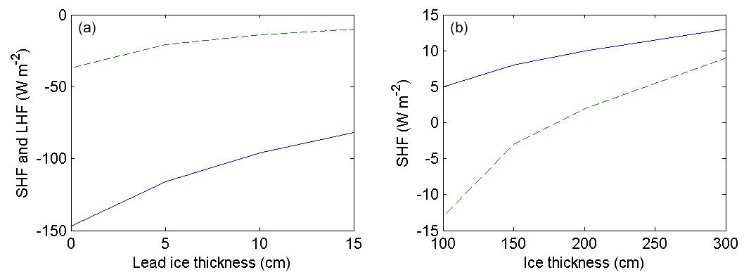
Figure 9(a) Effects of lead ice thickness on the SHF (solid line) and LHF (dashed line) on leads and (b) the effect of snow on top of thick sea ice on SHF (two cases are shown: 20 cm of snowpack on ice (solid line) and bare ice (dashed line)). The fluxes were calculated for February conditions as observed at the drifting ice station SHEBA (Persson et al., 2002).
Considering the effects of snowpack on top of thick sea ice, which are ignored in ERA5 and JRA-55, we again applied the SHEBA climatology for February and calculated the equilibrium net flux and its components for the cases of bare and snow-covered sea ice with a constant snow depth of 0.2 m and ice thicknesses of 1.0, 1.5, 2.0, and 3.0 m. In addition to the application of Eqs. (4) to (7), in the case of snow-covered ice, we calculated the conductive heat flux using a piecewise linear approximation (Makshtas, 1991):
where ks stands for the heat conductivity of the snow and hs for the snow thickness. The results suggest that for ice thicknesses of less than 2 m, the existence of the snowpack controls the direction of SHF: for 1 m sea ice, SHF is −13 W m−2 (upwards) without the snowpack but 5 W m−2 (downwards) with the snowpack (Fig. 9b). For larger ice thicknesses, the impact of the snowpack decreases as the insulating effect of the ice increases. In February conditions in the Central Arctic, the specific humidity and saturation specific humidity of the air over thick ice/snow are so small that LHF ranged between −1 and 1 W m−2 (not shown).
4.1 Differences between reanalyses, their importance, and consequences
In most Arctic basins, we found the highest SIC in NCEP/CFSR and JRA-55 data, whereas the values in ERA5 and MERRA-2 were lower and close to each other. The magnitude of the difference was up to 0.15 but typically around 0.05 (Fig. 2), similar to the average differences between reanalyses in the Arctic Ocean shown in Collow et al. (2020). Differences in SIC of the order of 0.05–0.15 may generate large differences in turbulent surface fluxes, and the magnitude of these differences depends on the sensitivity of the fluxes to SIC. Our results indicated that the highest sensitivity occurred in November–April (Figs. 4, 6, S4, and S7): approximately 400 W m−2 in LHF and over 800 W m−2 SHF per unit of SIC (change in SIC from 0 to 1). These values varied between the reanalyses – e.g. for LHF in November–December–January, they were approximately 200–300 W m−2 per unit of SIC in ERA5, JRA-55, and MERRA-2, whereas they were as large as up to 600 W m−2 LHF per unit of SIC in NCEP/CFSR data. In warmer seasons, the sensitivity of turbulent surface fluxes to SIC was generally lower.
The differences in LHF and SHF generated by differences in SIC and flux parameterisations have strong impacts on the atmosphere, especially in cold-season conditions (November–April), when the SIC is close to 1. According to modelling experiments by Lüpkes et al. (2008), in winter under clear skies, a SIC decrease of 1 % caused a T10 m increase of 3.5 K when an air mass flew long enough (48 h) over a zone with high SIC. During cold-air outbreaks from the Antarctic sea-ice zone, the modelled T2 m may vary by more than 10 K depending on the SIC algorithm applied, as seen in Fig. 7 in Valkonen et al. (2008). Warming of the near-surface temperature caused by a low sea-ice concentration then reduces the stratification in the Arctic atmospheric boundary layer and makes the atmosphere more prone to cyclogenesis (Jaiser et al., 2012). Such local and regional impacts in the sea-ice zone may have far-reaching effects beyond the polar regions. A sea-ice decline in the Arctic contributes to the Arctic amplification of climate warming, reducing the meridional temperature gradient between the Arctic and mid-latitudes. This impacts mid-latitude weather and climate, although the magnitude of the impacts and whether they can be distinguished from natural variability are still under debate (Cohen et al., 2020).
4.2 Simplification of the sea ice in reanalyses and its impact on surface turbulent fluxes
The SIC in reanalyses does not include information on the spatial distribution of sea ice and open water within a grid cell. For example, if SIC is 0.5, we do not know whether there is a distinct ice margin dividing the grid cell into equal portions of sea ice and open water or if there are numerous small leads whose total area sums to half of the grid cell. The impacts of the ice–water distribution on turbulent surface fluxes may depend on the season, region, and weather conditions via complex interactions of processes. In the case of cold-air outbreaks in cold seasons, when the sensitivity of SHF and LHF to SIC is largest, a distinct ice margin (with only sea ice on one side and only open water on the other side) typically results in a situation where SHF and LHF are largest right downwind of the ice margin and then decrease with fetch over the open ocean as the near-surface air becomes warmer and more humid (e.g. Lüpkes and Schlünzen, 1996). In a similar weather situation but with the SIC associated with a series of narrow leads, the near-surface air is not expected to get as warm and moist because part of the heat and moisture is returned to ice via downward turbulent fluxes over the patches of ice in between the leads, which allows larger SHF and LHF values over the leads. However, comparing the turbulent surface fluxes averaged over the grid cell between these two exemplary cases would require sophisticated large-eddy simulation experiments. A theoretical argument favouring larger grid-averaged fluxes in the latter case is that the alternations between the leads and sea ice increase the surface roughness due to the form drag generated by floe edges (Lüpkes and Gryanik, 2015). This enhances the turbulent transfer not only for momentum but also for sensible and latent heat (Elvidge et al., 2023). In any case, even if the reanalysis products were to include information on the spatial distributions of sea ice and open water within a grid cell, the SIC itself is an oversimplification of the true situation, as the sea ice in a grid cell typically has a range of thicknesses, each with different surface temperatures and, hence, SHF and LHF values.
The SIC in reanalyses is mostly based on satellite passive microwave data (Table 2). These data have a typical spatial resolution of the order of 10 to 30 km, depending on the wavelength band. Hence, the observations do not detect narrow leads. Further, any SIC based on satellite data is sensitive to the processing algorithm applied (Spreen et al., 2008) and includes errors, e.g. due to atmospheric disturbances (Svendsen et al., 1987). Other satellite-based SIC products, such as thermal infrared data (Qiu et al., 2023) and data from synthetic aperture radar (Park et al., 2020), are available at much higher spatial resolutions, with a pixel size of the order of tens of metres. However, the temporal and spatial coverage of these data sets is limited compared to the multi-decadal and global scales required for atmospheric reanalyses.
In addition to the uncertainty in SIC, there are also factors that generate errors in the turbulent fluxes over leads. A source of biases in SHF and LHF is the thin ice cover that is typically present on winter leads but ignored in reanalyses. According to our calculations, ignoring the thin ice may cause an overestimation of the heat loss from the lead by several tens of W m−2 in February conditions in the Central Arctic. In warmer seasons, the effect is naturally smaller, and it disappears in the peak of summer. Another source of biases in ERA5 and JRA-55 is the lack of snow on top of thick sea ice. Our calculations suggest that the local effect is smaller than that of the lack of thin ice on leads. However, as the lead fraction in the Central Arctic is small, we suppose that the regional effect of the lack of snow on thick sea ice is larger.
4.3 Other uncertainties in the parameterisation of surface turbulent fluxes
Even with perfect information on SIC, thin ice on leads, and the snow on top of ice, uncertainties are generated via the application of Eqs. (1) and (2). The numerical weather prediction (NWP) models used in the production of reanalyses have mutual differences in the height of the lowest atmospheric level. This height affects the differences between the atmospheric and surface values, and the lowest level should be located within a layer where the turbulent fluxes can be assumed constant in height. However, in stably stratified conditions, this layer is very shallow and often does not reach the lowest model level. In such cases, the Monin–Obukhov similarity theory (the basis for Eqs. 1 and 2) is not valid. Further, the vertical distributions of heat and moisture originating from leads (Lüpkes et al., 2012) cannot be correctly simulated if the model's vertical resolution is coarse. Stable stratification also generates a lot of uncertainty in the turbulent exchange coefficients for heat and moisture (Andreas et al., 2010; Grachev et al., 2012). In particular, the transition from weakly stable to very stable stratification results in a decrease in the magnitude of SHF even if the temperature difference between the air and the surface increases (Malhi, 1995), which may result in uncertainties of up to 10–20 K in T2 m (Uppala et al., 2005). Another uncertainty arises from the effect of form drag generated by flow edges, ridges, and sastrugi on the turbulent exchange coefficients (Andreas, 1995; Lüpkes and Gryanik, 2015; Elvidge et al., 2023). Finally, the flux parameterisation includes an error source related to the limited representativeness of the grid-averaged values of the air potential temperature, specific humidity, and wind speed for the local conditions over the ice-covered and open-water parts of the grid cell (Vihma et al., 1998).
Another issue in reanalyses is the very common warm bias in both Ts (Herrmannsdörfer et al., 2023) and T2 m (Graham et al., 2019), especially during clear-sky events in the cold season in the Arctic. If the biases in Ts and T2 m are approximately equal, the SHF over sea ice is not much affected. However, a positive T2 m bias reduces the temperature difference between the open water and the air above, resulting in the underestimation of upward turbulent fluxes over leads. In summer, the Ts over leads may be lower than T2 m, causing locally stable stratification. However, the summertime thermal differences between the atmosphere, sea ice, and leads are typically so small that the flux magnitudes and, hence, their absolute errors remain small. There is potential to reduce the biases in Ts, T2 m, SHF, and LHF by performing corrections via machine-learning algorithms trained by, for example, satellite observations of the ice surface temperatures, as shown in Zampieri et al. (2023).
4.4 Roles of the sea-ice concentration and meteorological variables in surface turbulent fluxes
Comparing the effects of SIC and other factors on LHF and SHF (Figs. 8, S10–S24), it is evident that air–surface differences in temperature and specific humidity explain the flux variations better than SIC does. This is natural, as the air–surface differences are the basis for flux parameterisations in models. However, SIC plays a key role in controlling the surface temperature and the surface (saturation) specific humidity, which have constant (freezing-point-related) values over areas of open water in the sea-ice zone (farther south, the sea-surface temperature may strongly exceed the freezing point). Accordingly, the air–surface differences in temperature and specific humidity are strongly affected by SIC. Wind speed explained only 10 % to 20 % of the turbulent surface flux variances, which we interpret as follows. Under constant air–surface differences in temperature and specific humidity, the magnitudes of turbulent fluxes increase with increasing wind speed, as seen from Eqs. (1) and (2). However, in upward-flux events, the wind effect results in decreased fluxes, whereas in downward-flux events, the fluxes increase. The cancelling effects then keep the above-mentioned partial R2 of the wind speed small. It does not vanish because events with a high air temperature and specific humidity over the Arctic Ocean typically occur under strong winds (Walsh and Chapman, 1998; Vihma and Pirazzini, 2005), favouring increases in the downward turbulent fluxes.
4.5 Decadal changes
As expected, all four reanalyses agreed that there was a general decrease in SIC over the 42-year study period. However, anomalies where SIC remained the same or became higher in the second study period (by up to 2 % of the value in 1980–2000) occurred in the Central Arctic and some of the adjacent seas in the cold season (November–April). These results are likely connected to the thinning of the Arctic sea ice in recent decades, which makes it more prone to ridging, rafting, and fast drift (Rampal et al., 2009). The exact mechanisms for the SIC increase remain unclear, but possibilities include a regionally increased convergence of ice drift associated with the closing of leads. Although the sea-ice decline has been very large in August–September–October in the Barents and Kara seas (Table 3), we did not detect the same or even a very minor signal in the decadal increases in negative LHF and SHF (Tables 4 and S1). We interpret this as being a consequence of increased transport of moist, warm air masses to the Arctic (Woods and Caballero, 2016), which are also associated with increasingly meridional cyclone tracks (Wickström et al., 2020). We found that the effects of SIC on both LHF and SHF weakened between the study periods in most areas of the Arctic, but mostly in the Central Arctic; however, we found areas with increased effects of SIC on LHF and SHF between 1980–2000 and 2001–2021. The mechanisms of these changes in the effects of SIC on turbulent surface fluxes are described in more detail in Sect. 3.2.
The results generally indicated signs of a decadal-scale improvement in the mutual agreement between reanalyses. The magnitudes of the mean biases in LHF and SHF between NCEP/CFSR and other reanalyses have decreased in nearly all basins and seasons. As the model and data assimilation system are the same over the entire reanalysis period, this better agreement may result from more data being available for assimilation. This must be mostly due to more available satellite data, as increases in the number of in situ observations from the Arctic have been restricted to short periods, such as the Year of Polar Prediction (YOPP) Special Observation Periods in February–March and July–September 2018 and the Multidisciplinary drifting Observatory for the Study of Arctic Climate (MOSAiC) field campaign in 2019–2020.
Our study expanded the knowledge of the effects of Arctic sea-ice concentration on the turbulent surface fluxes of sensible and latent heat, as represented in four global atmospheric reanalyses. We quantified the uncertainties in these effects, which arise from differences in SIC and in the sensitivities of the turbulent surface fluxes to SIC. Such analyses have not been performed before. Because atmospheric reanalyses provide the best available information for data-sparse regions such as the Arctic, and because the Arctic amplification of climate warming is thought to be primarily surface based, it is important to quantify the differences in the representation of the Arctic surface energy budget and its sensitivity to SIC in these data sets. In the present study, we showed that the largest differences in the effects of SIC on LHF and SHF in the reanalyses come from the representation of the sea ice, which is modelled in NCEP/CFSR and oversimplified in ERA5, JRA-55, and MERRA-2. This difference in representation of the sea ice generally resulted in a much higher sensitivity of turbulent surface fluxes to SIC in NCEP/CFSR (which assimilates both modelled sea-ice thickness and snow depth on the sea ice and accounts for their insulating effects) compared to other reanalyses (which assume a constant sea-ice thickness and do not account for the snow on sea ice). A logical next step in our work is to study the relationships of Arctic SIC and radiative surface fluxes and clouds in the atmospheric reanalyses ERA5, JRA-55, MERRA-2, and NCEP/CFSR.
The code and data used in this article are available at https://doi.org/10.5281/zenodo.7978071 (Uhlíková, 2023), https://doi.org/10.5281/zenodo.7965919 (Uotila, 2023), and https://a3s.fi/uhlitere-2000789-pub/* (last access: 25 February 2023) (Hersbach et al., 2023; Japan Meteorological Agency, 2013; GMAO, 2015a, b; Saha et al., 2010b, 2011). (To download a desired file, the name of it must be entered after the last forward slash, instead of *. Names of files can be found in codes or in the list of files at https://a3s.fi/swift/v1/AUTH_ea49151ae29449449d8e7cde1367e03a/uhlitere-2000789-pub/ (last access: 29 May 2023). A description of the data can be found at https://a3s.fi/uhlitere-2000789-pub/README_data.odt, last access: 29 May 2023.)
The supplement related to this article is available online at: https://doi.org/10.5194/tc-18-957-2024-supplement.
TU prepared the manuscript with contributions from TV, PU, and AYK. TV designed the concept of the study with contributions from PU, AYK, and TU. PU developed the code with a contribution from TU. TU collected and processed data and performed analyses.
The contact author has declared that none of the authors has any competing interests.
Neither the European Commission nor ECMWF is responsible for any use that may be made of the Copernicus information or data it contains.
Publisher's note: Copernicus Publications remains neutral with regard to jurisdictional claims made in the text, published maps, institutional affiliations, or any other geographical representation in this paper. While Copernicus Publications makes every effort to include appropriate place names, the final responsibility lies with the authors.
Hersbach et al. (2023) was downloaded from the Copernicus Climate Change Service (C3S) Climate Data Store. The results contain modified Copernicus Climate Change Service information 2022. Furthermore, we acknowledge the providers of the data in the other three reanalyses used in our study: the Japan Meteorological Agency, the National Center for Atmospheric Research (JRA-55, NCEP/CFSR, CFSv2), and the Global Modeling and Assimilation Office (MERRA-2).
Tereza Uhlíková is a university-funded doctoral researcher at the University of Helsinki. The work of Alexey Yu Karpechko, Petteri Uotila, and Timo Vihma was supported by the European Commission's Horizon 2020 Framework Programme (PolarRES; grant no. 101003590).
Open-access funding was provided by the Helsinki University Library.
This paper was edited by David Schroeder and reviewed by Evgenii Salganik and Zhaohui Wang.
Alam, A. and Curry, J.: Determination of surface turbulent fluxes over leads in Arctic sea ice, J. Geophys. Res., 102, 3331–3343, https://doi.org/10.1029/96JC03606, 1997. a
Andreas, E. L.: Air-ice drag coefficients in the western Weddell Sea: 2. A model based on form drag and drifting snow, J. Geophys. Res., 100, 4833–4843, https://doi.org/10.1029/94JC02016, 1995. a
Andreas, E. L., Paulson, C. A., William, R. M., Lindsay, R. W., and Businger, J. A.: The turbulent heat flux from arctic leads, Bound.-Lay. Meteorol., 17, 57–91, https://doi.org/10.1007/BF00121937, 1979. a
Andreas, E. L., Persson, P. O. G., Grachev, A. A., Jordan, R. E., Horst, T., Guest, P. S., and Fairall, C.: Parameterizing Turbulent Exchange over Sea Ice in Winter, J. Hydrometeorol, 11, 87–104, https://doi.org/10.1175/2009JHM1102.1, 2010. a
Aue, L., Vihma, T., Uotila, P., and Rinke, A.: New insights into cyclone impacts on sea ice in the Atlantic sector of the Arctic Ocean in winter, Geophys. Res. Lett., 49, e2022GL100051, https://doi.org/10.1029/2022GL100051, 2022. a
Boggs, P. T., Donaldson, J. T., Schnabel, R. B., and Spiegelman, C. H.: A Computational Examination of Orthogonal Distance Regression, J. Econom., 38, 169–201, 1988. a
Bosilovich, M. G., Akella, S., and Coy, L. E. A.: MERRA-2: Initial evaluation of the climate, https://gmao.gsfc.nasa.gov/pubs/docs/Bosilovich803.pdf (last access: ), 2015. a, b
Bretherton, C. S., Widmann, M., Dymnikov, V. P., Wallace, J. M., and Bladé, I.: The Effective Number of Spatial Degrees of Freedom of a Time-Varying Field, J. Climate, 12, 1990–2009, 1999. a
Claussen, M.: Local advection processes in the surface layer of the marginal ice zone, Bound.-Lay. Meteorol., 54, 1–27, https://doi.org/10.1007/BF00119409, 1991. a
Cohen, J., Zhang, X., Francis, J., Jung, T., Kwok, R., Overland, J., Ballinger, T. J., Bhatt, U. S., Chen, H. W., Coumou, D., Feldstein, S., Gu, H., Handorf, D., Henderson, G., Ionita, M., Kretschmer, M., Laliberte, F., Lee, S., Linderholm, H. W., Maslowski, W., Peings, Y., Pfeiffer, K., Rigor, I., Semmler, T., Stroeve, J., Taylor, P. C., Vavrus, S., Vihma, T., Wang, S., Wendisch, M., Wu, Y., and Yoon, J.: Divergent consensuses on Arctic amplification influence on midlatitude severe winter weather, Nat. Clim. Change, 10, 20–29, https://doi.org/10.1038/s41558-019-0662-y, 2020. a
Collow, A. B. M., Cullather, R. I., and Bosilovich, M. G.: Recent Arctic Ocean Surface Air Temperatures in Atmospheric Reanalyses and Numerical Simulations, J. Climate, 33, 4347–4367, 2020. a, b
Dai, A., Luo, D., Song, M., and Liu, J.: Arctic amplification caused by sea-ice loss under increasing CO2, Nat. Commun., 10, 121, https://doi.org/10.1038/s41467-018-07954-9, 2002. a
ECMWF: IFS Documentation CY41R2 – Part IV: Physical Processes, 4, ECMWF, https://doi.org/10.21957/tr5rv27xu, 2016. a
Elvidge, A. D., Renfrew, I. A., Edwards, J. M., Brooks, I. M., Srivastava, P., and Weiss, A. I.: Improved simulation of the polar atmospheric boundary layer by accounting for aerodynamic roughness in the parameterization of surface scalar exchange over sea ice, J. Adv. Model. Earth Sy., 15, e2022MS003305, https://doi.org/10.1029/2022MS003305, 2023. a, b
Gelaro, R., McCarthy, W., and Suárez, M. J. E. A.: The Modern-Era Retrospective Analysis for Research and Applications, Version 2 (MERRA-2), J. Climate, 30, 5419–5454, 2017. a, b, c
Global Modeling and Assimilation Office (GMAO): Tavg1_2d_flx_Nx: MERRA-2 2D, 1-Hourly, Time-Averaged, Single-Level Assimilation, Single-Level Diagnostics, Greenbelt, MD, USA, Goddard Earth Sciences Data and Information Services Center (GES DISC) [data set], https://doi.org/10.5067/7MCPBJ41Y0K6, 2015a. a, b
Global Modeling and Assimilation Office (GMAO): Tavg1_2d_slv_Nx: MERRA-2 2D, 1-hourly, Time-Averaged, Single-Level Assimilation,Surface Flux Diagnostics V5.12.4, Greenbelt, MD, USA, Goddard Earth Sciences Data and Information Services Center (GES DISC) [data set], https://doi.org/10.5067/VJAFPLI1CSIV, 2015b. a, b
Good, S., Fiedler, E., Mao, C., Martin, M. J., Maycock, A., Reid, R., Roberts-Jones, J., Searle, T., Waters, J., While, J., and Worsfold, M.: The Current Configuration of the OSTIA System for Operational Production of Foundation Sea Surface Temperature and Ice Concentration Analyses, Remote Sens., 12, 720, https://doi.org/10.3390/rs12040720, 2020. a
Grachev, A. A., Andreas, E. L., Fairall, C., Guest, P. S., and Persson, P. O. G.: Outlier problem in evaluating similarity functions in the stable atmospheric boundary layer, Bound.-Layer Meteorol., 144, 137–155, 2012. a
Graham, R. M., Cohen, L., Ritzhaupt, N., Segger, B., Graversen, R. G., Rinke, A., Walden, V. P., Granskog, M. A., and Hudson, S. R.: Evaluation of Six Atmospheric Reanalyses over Arctic Sea Ice from Winter to Early Summer, J. Climate, 32, 4121–4143, https://doi.org/10.1175/JCLI-D-18-0643.1, 2019. a, b, c
Gultepe, I., Isaac, G. A., Williams, A., Marcotte, D., and Strawbridge, K. B.: Turbulent heat fluxes over leads and polynyas, and their effects on arctic clouds during FIRE.ACE: Aircraft observations for April 1998, Atmosphere-Ocean, 41, 15–34, https://doi.org/10.3137/ao.410102, 2003. a
Herrmannsdörfer, L., Müller, M., Shupe, M. D., and Rostosky, P.: Surface temperature comparison of the Arctic winter MOSAiC observations, ERA5 reanalysis, and MODIS satellite retrieval, Elementa: Science of the Anthropocene, 11, 00085, https://doi.org/10.1525/elementa.2022.00085, 2023. a
Hersbach, H., Bell, B., Berrisford, P., Hirahara, S., Horányi, A., Muñoz Sabater, J., Nicolas, J., Peubey, C., Radu, R., Schepers, D., Simmons, A., Soci, C., Abdalla, S., Abellan, X., Balsamo, G., Bechtold, P., Biavati, G., Bidlot, J., Bonavita, M., and Thépaut, J.-N.: The ERA5 global reanalysis, Q. J. Roy. Meteor. Soc., 146, 1999–2495, https://doi.org/10.1002/qj.3803, 2020. a, b
Hersbach, H., Bell, B., Berrisford, P., Biavati, G., Horányi, A., Muñoz Sabater, J., Nicolas, J., Peubey, C., Radu, R., Rozum, I., Schepers, D., Simmons, A., Soci, C., Dee, D., and Thépaut, J.-N.: ERA5 hourly data on single levels from 1940 to present, Copernicus Climate Change Service (C3S) Climate Data Store (CDS) [data set], https://doi.org/10.24381/cds.adbb2d47, 2023. a, b, c
Iribarne, J. and Godson, W.: Atmospheric Thermodynamics, D. Reidel Publishing Company, 1973. a
Ishii, M., Shouji, A., Sugimoto, S., and Matsumoto, T.: Objective analyses of sea-surface temperature and marine meteorological variables for the 20th century using ICOADS and the Kobe Collection, Int. J. Climatol., 25, 865–879, https://doi.org/10.1002/joc.1169, 2005. a
Jaiser, R., Dethloff, K., Handorf, D., and Cohen, J.: Impact of sea ice cover changes on the Northern Hemisphere atmospheric winter circulation, Tellus A, 64, 11595, https://doi.org/10.3402/tellusa.v64i0.11595, 2012. a
Japan Meteorological Agency: JRA-55: Japanese 55-year Reanalysis, Daily 3-Hourly and 6-Hourly Data, Research Data Archive at the National Center for Atmospheric Research, Computational and Information Systems Laboratory [data set], https://doi.org/10.5065/D6HH6H41, 2013. a, b
Kobayashi, S., Ota, Y., and Harada, Y. E. A.: The JRA-55 Reanalysis: General Specifications and Basic Characteristics, J. Meteorol. Soc. Jpn., 93, 5–48, https://doi.org/10.2151/JMSJ.2015-001, 2015. a, b, c
Koster, R. D. and Suarez, M. J.: Modeling the land surface boundary in climate models as a composite of independent vegetation stands, J. Geophys. Res., 97, 2697–2715, 1992. a
Lim, W.-I., Park, H.-S., Stewart, A. L., and Seo, K.-H.: Suppression of Arctic sea ice growth in the Eurasian–Pacific seas by winter clouds and snowfall, J. Climate, 35, 669–686, https://doi.org/10.1175/JCLI-D-21-0282.1, 2022. a
Lindsay, R., Wensnahan, M., Schweiger, A., and Zhang, J.: Evaluation of Seven Different Atmospheric Reanalysis Products in the Arctic, J. Climate, 27, 2588–2606, https://doi.org/10.1175/JCLI-D-13-00014.1, 2014. a
Lüpkes, C. and Gryanik, V.: A stability-dependent parametrization of transfer coefficients for momentum and heat over polar sea ice to be used in climate models, J. Geophys. Res., 120, 552–581, https://doi.org/10.1002/2014JD022418, 2015. a, b
Lüpkes, C. and Schlünzen, K. H.: Modelling the Arctic Convective Boundary-Layer with Different Turbulence Parameterizations, Bound.-Lay. Meteorol., 79, 107–130, 1996. a
Lüpkes, C., Vihma, T., Birnbaum, G., and Wacker, U.: Influence of leads in sea ice on the temperature of the atmospheric boundary layer during polar night., Geophys. Res. Lett., 35, L03805, https://doi.org/10.1029/2007GL032461, 2008. a, b
Lüpkes, C., Vihma, T., Birnbaum, G., Dierer, S., Garbrecht, T., Gryanik, V., Gryschka, M., Hartmann, J., Heinemann, G., Kaleschke, L., Raasch, S., Savijärvi, H., Schlünzen, K., and Wacker, U.: Mesoscale modelling of the Arctic atmospheric boundary layer and its interaction with sea ice, in: Arctic Climate Change - The ACSYS Decade and Beyond, edited by: Lemke, P. and Jacobi, H.-W., vol. 43, Atmospheric and Oceanographic Sciences Library, 2012. a
Makshtas, A. P.: The heat budget of the Arctic ice in the winter, Cambridge, International Glaciological Society, edited by: Andreas, E. L., ISBN 0 946417 12 1, 1991. a, b
Maksimovich, E. and Vihma, T.: The effect of surface heat fluxes on interannual variability in the spring onset of snow melt in the central Arctic Ocean, J. Geophys. Res.-Oceans, 117, C07012, https://doi.org/10.1029/2011JC007220, 2012. a
Malhi, Y. S.: The significance of the dual solutions for heat fluxes measured by the temperature fluctuation method in stable conditions, Bound.-Lay. Meteorol., 74, 389–396, 1995. a
Matsumoto, T., Ishii, M., Fukuda, Y., and Hirahara, S.: Sea ice data derived from microwave radiometer for climate monitoring, Proceedings of the 14th Conference on Satellite Meteorology and Oceanography, Atlanta, USA, in: Presented at the 14th Conference on Satellite Meteorology and Oceanography, https://ams.confex.com/ams/Annual2006/techprogram/paper_101105.htm (last access: 27 May 2023), 2006. a
Michaelis, J., Lüpkes, C., Schmitt, A., and Hartmann, J.: Modelling and parametrization of the convective flow over leads in sea ice and comparison with airborne observations, Q. J. Roy. Meteor. Soc., 147, 914–943, https://doi.org/10.1002/qj.3953, 2021. a
Morice, C. P., Kennedy, J. J., Rayner, N. A., W., P., J., Hogan, E., and Killick, R. E. E. A.: An updated assessment of near-surface temperature change from 1850: the HadCRUT5 data set, J. Geophys. Res.-Atmos., 126, e2019JD032361, https://doi.org/10.1029/2019JD032361, 2021. a
Overland, J. E., McNutt, S. L., Groves, J., Salo, S., Andreas, E. L., and Persson, P. O. G.: Regional sensible and radiative heat flux estimates for the winter arctic during the Surface Heat Budget of the Arctic Ocean (SHEBA) experiment, J. Geophys. Res., 105, 14093–14102, 2000. a
Park, J.-W., Korosov, A. A., Babiker, M., Won, J.-S., Hansen, M. W., and Kim, H.-C.: Classification of sea ice types in Sentinel-1 synthetic aperture radar images, The Cryosphere, 14, 2629–2645, https://doi.org/10.5194/tc-14-2629-2020, 2020. a
Perovich, D. K., Light, B., Eicken, H., Jones, K. F., Runciman, K., and Nghiem, S. V.: Increasing solar heating of the Arctic Ocean and adjacent seas, 1979–2005: Attribution and role in the ice-albedo feedback, Geophys. Res. Lett., 34, https://doi.org/10.1029/2007GL031480, 2007. a
Persson, P. O. G., Fairall, C. W., Andreas, E. L., Guest, P. S., and Perovich, D. K.: Measurements near the Atmospheric Surface Flux Group tower at SHEBA: Near-surface conditions and surface energy budget, J. Geophys. Res., 107, 8045, https://doi.org/10.1029/2000JC000705, 2002. a, b, c, d
Petrich, C., Langhorne, P. J., and Haskell, T. G.: Formation and structure of refrozen cracks in land-fast first-year sea ice, J. Geophys. Res., 112, C04006, https://doi.org/10.1029/2006JC003466, 2007. a
Qiu, Y., Li, X.-M., and Guo, H.: Spaceborne thermal infrared observations of Arctic sea ice leads at 30 m resolution, The Cryosphere, 17, 2829–2849, https://doi.org/10.5194/tc-17-2829-2023, 2023. a
Rampal, P., Weiss, J., and Marsan, D.: Positive trend in the mean speed and deformation rate of Arctic sea ice: 1979–2007, J. Geophys. Res., 114, C05013, https://doi.org/10.1029/2008JC005066, 2009. a
Saha, S., Moorthi, S., Pan, H.-L., Wu, X., Wang, J., Nadiga, S., Tripp, P., Kistler, R., Woollen, J., Behringer, D., Liu, H., Stokes, D., Grumbine, R., Gayno, G., Wang, J., Hou, Y.-T., Chuang, H.-Y., Juang, H.-M., Sela, J., and Goldberg, M.: The NCEP climate forecast system reanalysis, B. Am. Meteorol. Soc., 91, 1015–1058, https://doi.org/10.1175/2010BAMS3001.1, 2010a. a
Saha, S., Moorthi, S., Pan, H.-L., Wu, X., Wang, J., Nadiga, S., Tripp, P., Kistler, R., Woollen, J., Behringer, D., Liu, H., Stokes, D., Grumbine, R., Gayno, G., Wang, J., Hou, Y.-T., Chuang, H.-Y., Juang, H.-M. H., Sela, J., Iredell, M., Treadon, R., Kleist, D., Van Delst, P., Keyser, D., Derber, J., Ek, M., Meng, J., Wei, H., Yang, R., Lord, S., van den Dool, H., Kumar, A., Wang, W., Long, C., Chelliah, M., Xue, Y., Huang, B., Schemm, J.-K., Ebisuzaki, W., Lin, R., Xie, P., Chen, M., Zhou, S., Higgins, W., Zou, C.-Z., Liu, Q., Chen, Y., Han, Y., Cucurull, L., Reynolds, R. W., Rutledge, G., and Goldberg, M.: NCEP Climate Forecast System Reanalysis (CFSR) 6-hourly Products, January 1979 to December 2010, Research Data Archive at the National Center for Atmospheric Research, Computational and Information Systems Laboratory [data set], https://doi.org/10.5065/D69K487J, 2010b. a, b
Saha, S., Moorthi, S., Pan, H.-L., Wu, X., Wang, J., Nadiga, S., Tripp, P., Kistler, R., Woollen, J., Behringer, D., Liu, H., Stokes, D., Grumbine, R., Gayno, G., Wang, J., Hou, Y.-T., Chuang, H.-Y., Juang, H.-M. H., Sela, J., Iredell, M., Treadon, R., Kleist, D., Van Delst, P., Keyser, D., Derber, J., Ek, M., Meng, J., Wei, H., Yang, R., Lord, S., van den Dool, H., Kumar, A., Wang, W., Long, C., Chelliah, M., Xue, Y., Huang, B., Schemm, J.-K., Ebisuzaki, W., Lin, R., Xie, P., Chen, M., Zhou, S., Higgins, W., Zou, C.-Z., Liu, Q., Chen, Y., Han, Y., Cucurull, L., Reynolds, R. W., Rutledge, G., and Goldberg, M.: NCEP Climate Forecast System Version 2 (CFSv2) 6-hourly Products, Research Data Archive at the National Center for Atmospheric Research, Computational and Information Systems Laboratory [data set], https://doi.org/10.5065/D61C1TXF, 2011. a, b
Saha, S., Moorthi, S., Wu, X., Wang, J., Nadiga, S., Tripp, P., Behringer, D., Hou, Y.-T., ya Chuang, H., Iredell, M., Ek, M., Meng, J., Yang, R., Mendez, M. P., van den Dool, H., Zhang, Q., Wang, W., Chen, M., and Becker, E.: The NCEP Climate Forecast System Version 2, J. Climate, 27, 2185–2208, 2014. a
Screen, J. A. and Simmonds, I.: The central role of diminishing sea ice in recent Arctic temperature amplification, Nature, 646, 1334–1337, https://doi.org/10.1038/nature09051, 2010. a
Serreze, M. C., Barrett, A. P., Stroeve, J. C., Kindig, D. N., and Holland, M. M.: The emergence of surface-based Arctic amplification, The Cryosphere, 3, 11–19, https://doi.org/10.5194/tc-3-11-2009, 2009. a
Spreen, G., Kaleschke, L., and Heygster, G.: Sea ice remote sensing using AMSR-E 89-GHz channels, J. Geophys. Res., 113, C02S03, https://doi.org/10.1029/2005JC003384, 2008. a
Svendsen, E., Matzler, C., and Grenfell, T. C.: A model for retrieving total sea ice concentration from a spaceborne dual-polarized passive microwave instrument operating near 90 GHz, Int J. Remote Sens., 8, 1479–1487, https://doi.org/10.1080/01431168708954790, 1987. a
Taylor, K. E., Williamson, D., and Zwiers, F.: The sea surface temperature and sea-ice concentration boundary conditions for AMIP II simulations, in: PCMDI Report No. 60, https://pcmdi.llnl.gov/report/ab60.html (last access: 27 March 2023), 2000. a
Tsamados, M., Feltham, D., Petty, A., Schroeder, D., and Flocco, D.: Processes controlling surface, bottom and lateral melt of Arctic sea ice in a state of the art sea ice model, Philos. T. Roy. Soc. A, 373, 20140167, https://doi.org/10.1098/rsta.2014.0167, 2015. a
Uhlíková, T.: Effects of Arctic sea-ice concentration on turbulent surface fluxes in four atmospheric reanalyses, Zenodo [code], https://doi.org/10.5281/zenodo.7978071, 2023. a
Uotila, P.: puotila/odrfitf902py: version 1.0 (v1.0.0), Zenodo [code], https://doi.org/10.5281/zenodo.7965919, 2023. a
Uppala, S. M., KÅllberg, P. W., Simmons, A. J., Andrae, U., Bechtold, V. D. C., Fiorino, M., Gibson, J. K., Haseler, J., Hernandez, A., Kelly, G. A., Li, X., Onogi, K., Saarinen, S., Sokka, N., Allan, R. P., Andersson, E., Arpe, K., Balmaseda, M. A., Beljaars, A. C. M., Berg, L. V. D., Bidlot, J., Bormann, N., Caires, S., Chevallier, F., Dethof, A., Dragosavac, M., Fisher, M., Fuentes, M., Hagemann, S., Hólm, E., Hoskins, B. J., Isaksen, L., Janssen, P. A. E. M., Jenne, R., Mcnally, A. P., Mahfouf, J.-F., Morcrette, J.-J., Rayner, N. A., Saunders, R. W., Simon, P., Sterl, A., Trenberth, K. E., Untch, A., Vasiljevic, D., Viterbo, P., and Woollen, J.: The ERA-40 reanalysis, Q. J. Roy. Meteor. Soc., 131, 2961–3012, https://doi.org/10.1256/qj.04.176, 2005. a
Valkonen, T., Vihma, T., and Doble, M.: Mesoscale modelling of the atmospheric boundary layer over the Antarctic sea ice: a late autumn case study, Mon. Weather Rev., 136, 1457–1474, 2008. a, b
Vihma, T.: Subgrid parameterization of surface heat and momentum fluxes over polar oceans, J. Geophys. Res., 100, 22625–22646, https://doi.org/10.1029/95JC02498, 1995. a
Vihma, T. and Pirazzini, R.: On the factors controlling the snow surface and 2-m air temperatures over the Arctic sea ice in winter, Bound.-Lay. Meteorol., 117, 73–90, 2005. a
Vihma, T., Uotila, J., and Launiainen, J.: Air-sea interaction over a thermal marine front in the Denmark Strait, J. Geophys. Res., 103, 27665–27678, https://doi.org/10.1029/98JC02415, 1998. a
Vihma, T., Jaagus, J., Jakobson, E., and Palo, T.: Meteorological conditions in the Arctic Ocean in spring and summer 2007 as recorded on the drifting ice station Tara, Geophys. Res. Lett., 35, L18706, https://doi.org/10.1029/2008GL034681, 2008. a
Walden, V. P., Hudson, S. R., Cohen, L., Murph, S. Y., and Granskog, M. A.: Atmospheric components of the surface energy budget over young sea ice: Results from the N-ICE2015 campaign., J. Geophys. Res.-Atmos., 122, 8427–8446, https://doi.org/10.1002/2016JD026091, 2017. a, b
Walsh, J. E. and Chapman, W. L.: Arctic Cloud–Radiation–Temperature Associations in Observational Data and Atmospheric Re-analyses, J. Climate, 11, 3030–3045, 1998. a
Wei, Z., Zhang, Z., Vihma, T., Wang, X., and Chen, Y.: An overview of Antarctic polynyas: sea ice production, forcing mechanisms, temporal variability and water mass formation, Adv. Polar Sci., 32, 295–311, https://doi.org/10.13679/j.advps.2021.0026, 2021. a
Wickström, S., Jonassen, M., Cassano, J. J., and Vihma, T.: Present temperature, precipitation and rain-on-snow climate in Svalbard, J. Geophys. Res.-Atmos., 125, e2019JD032155, https://doi.org/10.1029/2019JD032155, 2020. a
Woods, C. and Caballero, R.: The role of moist intrusions in winter Arctic warming and sea ice decline, J. Climate, 29, 4473–4485, https://doi.org/10.1175/JCLI-D-15-0773.1, 2016. a
Zampieri, L., Arduini, G., Holland, M., Keeley, S. P. E., Mogensen, K., Shupe, M. D., and Tietsche, S.: A Machine Learning Correction Model of the Winter Clear-Sky Temperature Bias over the Arctic Sea Ice in Atmospheric Reanalyses., Mon. Weather Rev., 151, 1443–1458, https://doi.org/10.1175/MWR-D-22-0130.1, 2023. a