the Creative Commons Attribution 4.0 License.
the Creative Commons Attribution 4.0 License.
 | 28 Feb 2024
Local forcing mechanisms challenge parameterizations of ocean thermal forcing for Greenland tidewater glaciers
David A. Sutherland
Donald A. Slater
Frontal ablation has caused 32 %–66 % of Greenland Ice Sheet mass loss since 1972, and despite its importance in driving terminus change, ocean thermal forcing remains crudely incorporated into large-scale ice sheet models. In Greenland, local fjord-scale processes modify the magnitude of thermal forcing at the ice–ocean boundary but are too small scale to be resolved in current global climate models. For example, simulations used in the Ice Sheet Intercomparison Project for CMIP6 (ISMIP6) to predict future ice sheet change rely on the extrapolation of regional ocean water properties into fjords to drive terminus ablation. However, the accuracy of this approach has not previously been tested due to the scarcity of observations in Greenland fjords, as well as the inability of fjord-scale models to realistically incorporate icebergs. By employing the recently developed IceBerg package within the Massachusetts Institute of Technology general circulation model (MITgcm), we here evaluate the ability of ocean thermal forcing parameterizations to predict thermal forcing at tidewater glacier termini. This is accomplished through sensitivity experiments using a set of idealized Greenland fjords, each forced with equivalent ocean boundary conditions but with varying tidal amplitudes, subglacial discharge, iceberg coverage, and bathymetry. Our results indicate that the bathymetric obstruction of external water is the primary control on near-glacier thermal forcing, followed by iceberg submarine melting. Despite identical ocean boundary conditions, we find that the simulated fjord processes can modify grounding line thermal forcing by as much as 3 °C, the magnitude of which is largely controlled by the relative depth of bathymetric sills to the Polar Water–Atlantic Water thermocline. However, using a common adjustment for fjord bathymetry we can still predict grounding line thermal forcing within 0.2 °C in our simulations. Finally, we introduce new parameterizations that additionally account for iceberg-driven cooling that can accurately predict interior fjord thermal forcing profiles both in iceberg-laden simulations and in observations from Kangiata Sullua (Ilulissat Icefjord).
- Article
(2204 KB) - Full-text XML
- BibTeX
- EndNote


Mass loss from the Greenland Ice Sheet (GrIS) contributed 10.8 ± 0.9 mm to mean sea level rise from 1992 to 2018 (The IMBIE Team, 2019) and is projected to raise sea level by 90–180 mm by 2100 (Fox-Kemper et al., 2021). This mass loss has, in part, been triggered by the tidewater glacier response to warming ocean temperatures (e.g., Nick et al., 2009; Holland et al., 2008; Murray et al., 2010; Motyka et al., 2011; Straneo and Heimbach, 2013; Wood et al., 2018), with frontal ablation accounting for 32 %–66 % of GrIS mass loss since 1972 (Enderlin et al., 2014; Van den Broeke et al., 2016; Mouginot et al., 2019). In Greenland, fjords are the principal pathways connecting tidewater glacier termini to the coastal ocean, in which local processes relating to sill-driven mixing and silled obstruction of external water (Mortensen et al., 2011, 2013, 2014; Moffat et al., 2018; Jakobsson et al., 2020; Hager et al., 2022), submarine melting of icebergs and glacier termini (Davison et al., 2020; Jackson et al., 2020; Magorrian and Wells, 2016; Moon et al., 2018), and subglacial discharge (Carroll et al., 2015; Jenkins, 2011) modulate the magnitude of ocean forcing at the ice–ocean boundary, often on a seasonal basis (e.g., Moffat et al., 2018; Mortensen et al., 2013; Hager et al., 2022). However, such processes are too small scale (∼ 1 m to ∼ 1 km length scales at hourly to seasonal timescales) to be resolved in global climate models (grid resolutions of ∼ 30–60 km at annual timescales; e.g., Watanabe et al., 2010; Golaz et al., 2019). To date, sea level rise projections have instead relied on poorly validated simplified parameterizations of oceanic boundary conditions in ice sheet models – such as those developed in Morlighem et al. (2019), Jourdain et al. (2020), and Slater et al. (2020) – that are large sources of uncertainty when predicting future mean sea level (Goelzer et al., 2020; Seroussi et al., 2020). This paper focuses on the ocean thermal forcing of GrIS outlet glaciers, yet Antarctic ice sheet models face similar challenges when prescribing ocean boundary conditions beneath ice shelves (e.g., Seroussi et al., 2020; Jourdain et al., 2020; Burgard et al., 2022).
Recent studies have shown that multi-decadal retreat across a population of tidewater glaciers can be reasonably approximated as a linear function of the climate forcing they experience (Cowton et al., 2018; Slater et al., 2019; Fahrner et al., 2021; Black and Joughin, 2022). For many Greenland tidewater glaciers, change in terminus position is specifically thought to be the result of enhanced submarine melting of the terminus and subsequent changes to ice dynamics (e.g., Holland et al., 2008; Murray et al., 2010; Straneo and Heimbach, 2013; Luckman et al., 2015). Taken together, these findings have prompted the development of parameterizations that use submarine melting to drive frontal ablation in ice sheet models. In particular, the Ice Sheet Intercomparison Project for CMIP6 (Coupled Model Intercomparison Project; ISMIP6) (Nowicki et al., 2016, 2020), which produced sea level contribution projections for Greenland in the Sixth Assessment Report of the Intergovernmental Panel on Climate Change (IPCC, 2023), relies on two such parameterizations. The first parameterization (called the retreat implementation) is the simplest – being designed to be implementable in all participating ISMIP6 models – and is used to determine changes in the glacier terminus position over a given time (Slater et al., 2019, 2020):
where ΔL is the retreat/advance distance (km) between times t1 and t2, Q is the mean summer subglacial discharge, Θ is the ocean thermal forcing (°C above freezing temperature), and κ is a coefficient tuned to fit the observed terminus positions of almost 200 Greenland tidewater glaciers between 1960–2018 (Slater et al., 2019). Here, submarine melting is assumed to scale proportionally to Q0.4Θ.
The second parameterization, called the submarine melt implementation, encompasses only submarine melt and leaves the subsequent glacier response (as given by the relationship between ice flux, submarine melt, and calving) to be calculated by the ice sheet model (e.g., Morlighem et al., 2016). Here, submarine melt rate () is (Rignot et al., 2016)
where h is grounding line depth and q is the annual mean subglacial discharge normalized by the calving front area. In both implementations, ice sheet models need a method for prescribing Θ based on offshore ocean conditions. In ISMIP6, this was done by first taking a spatial average of annual mean ocean conditions within seven large regional zones surrounding Greenland (Slater et al., 2020). For the retreat implementation (Eq. 1), glaciers are forced with a depth-averaged Θ so that all glaciers within a region experience the same thermal forcing. In the submarine melt implementation (Eq. 2), an adjustment is made accounting for fjord bathymetry preventing deep currents from reaching the glacier face (Sect. 2.2; Morlighem et al., 2019). However, neither parameterization explicitly incorporates water transformation between the coast and glacier termini (e.g., Gladish et al., 2015; Straneo et al., 2012), which can vary greatly even between neighboring fjords (Bartholomaus et al., 2016). Furthermore, accelerated mass loss from the Greenland Ice Sheet can be largely attributed to the dynamics of only a small number of individual glaciers (Enderlin et al., 2014; Fahrner et al., 2021), which can dominate uncertainty in regional retreat projections (Goelzer et al., 2020). There is thus an urgent need for improved parameterizations that incorporate local water transformation and that are validated by high-resolution models or extensive observations.
The large-scale and long-term observations necessary to validate such parameterizations are logistically difficult in Greenland, suggesting a modeling approach is warranted. However, until recently, general circulation models lacked the ability to realistically incorporate iceberg melting, which can be the primary freshwater source in Greenland fjords (Enderlin et al., 2016; Moon et al., 2018). Here, we employ the newly developed IceBerg package (Davison et al., 2020) within the Massachusetts Institute of Technology general circulation model (MITgcm) (Marshall et al., 1997) that enables the inclusion of icebergs to test the accuracy of both ISMIP6 thermal forcing parameterizations across a variety of local forcing conditions. We create a suite of idealized model simulations, each forced with different combinations of subglacial discharge, iceberg prevalence, tidal forcing, and sill geometry but all experiencing the same offshore temperature and salinity conditions at the open boundary. In doing so, our objective is to simulate the diverse array of neighboring fjord conditions that can result from the same regional ocean forcing when local factors are accounted for. We then quantify the error of each ISMIP6 thermal forcing parameterization for all model runs and determine the primary contributors to local water transformation and uncertainty within each formulation. Based on our results, we recommend simple improvements to current thermal forcing parameterizations that substantially improve their accuracy. This paper focuses solely on the accuracy of thermal forcing parameterizations, while assessing the validity of Eqs. (1) and (2), which are provided here only for context, is left to other studies.
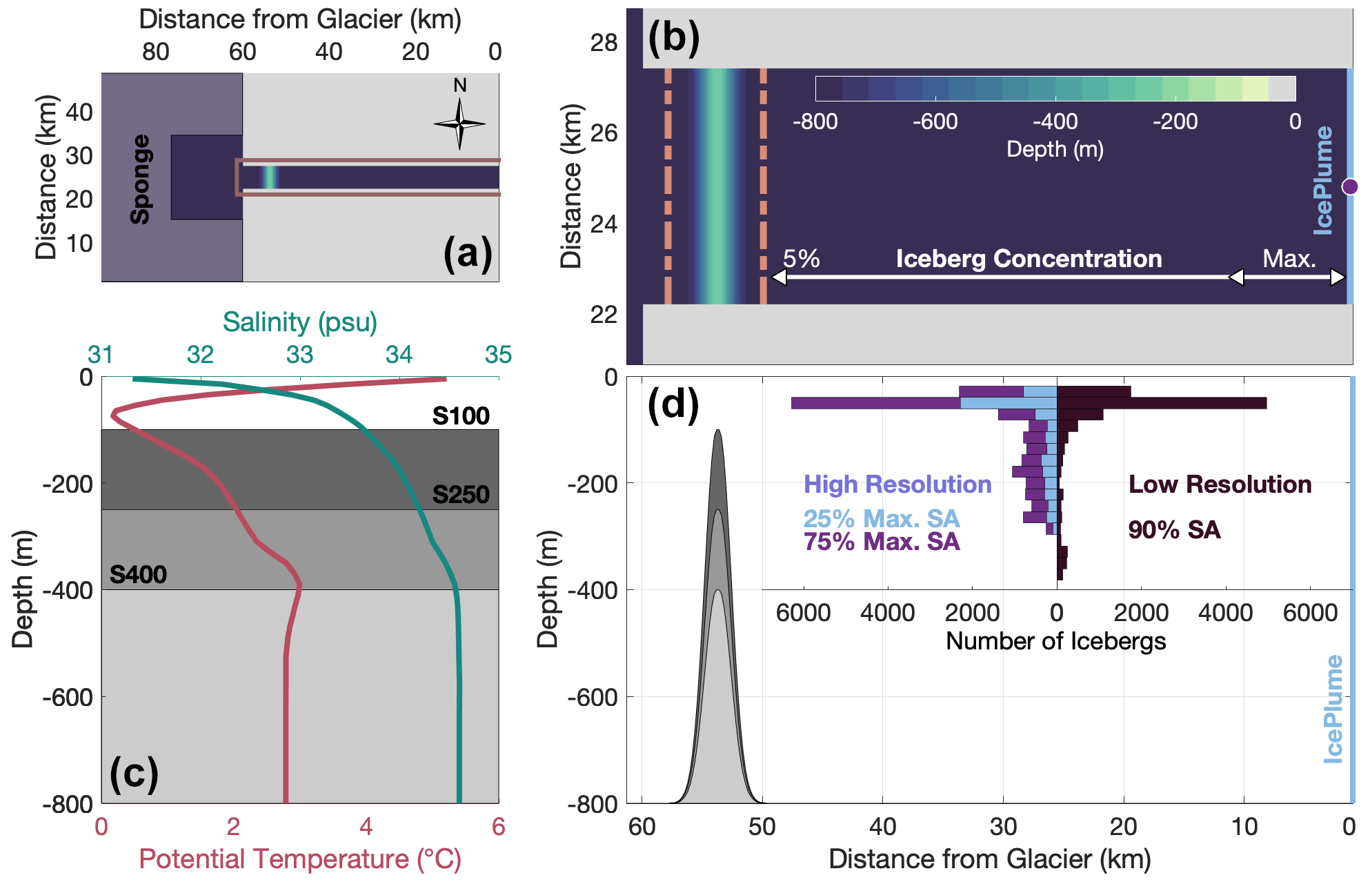
Figure 1(a) Model domain with the location of the sponge layer along open boundaries. (b) Enlargement of the brown box in (a) depicting the locations of the entrance sill, total exchange flow transects (dashed lines), glacier face (blue line), subglacial discharge plume center point (purple dot), and the distribution of iceberg concentrations. (c) Initial and open boundary conditions in relation to the depths of each sill. (d) Along-fjord cross-section of (b) depicting the vertical distribution of iceberg keel depths (binned every 25 m) for each iceberg scenario (labeled by the maximum coverage of grid cell surface area, SA), plotted with the depths of each sill.
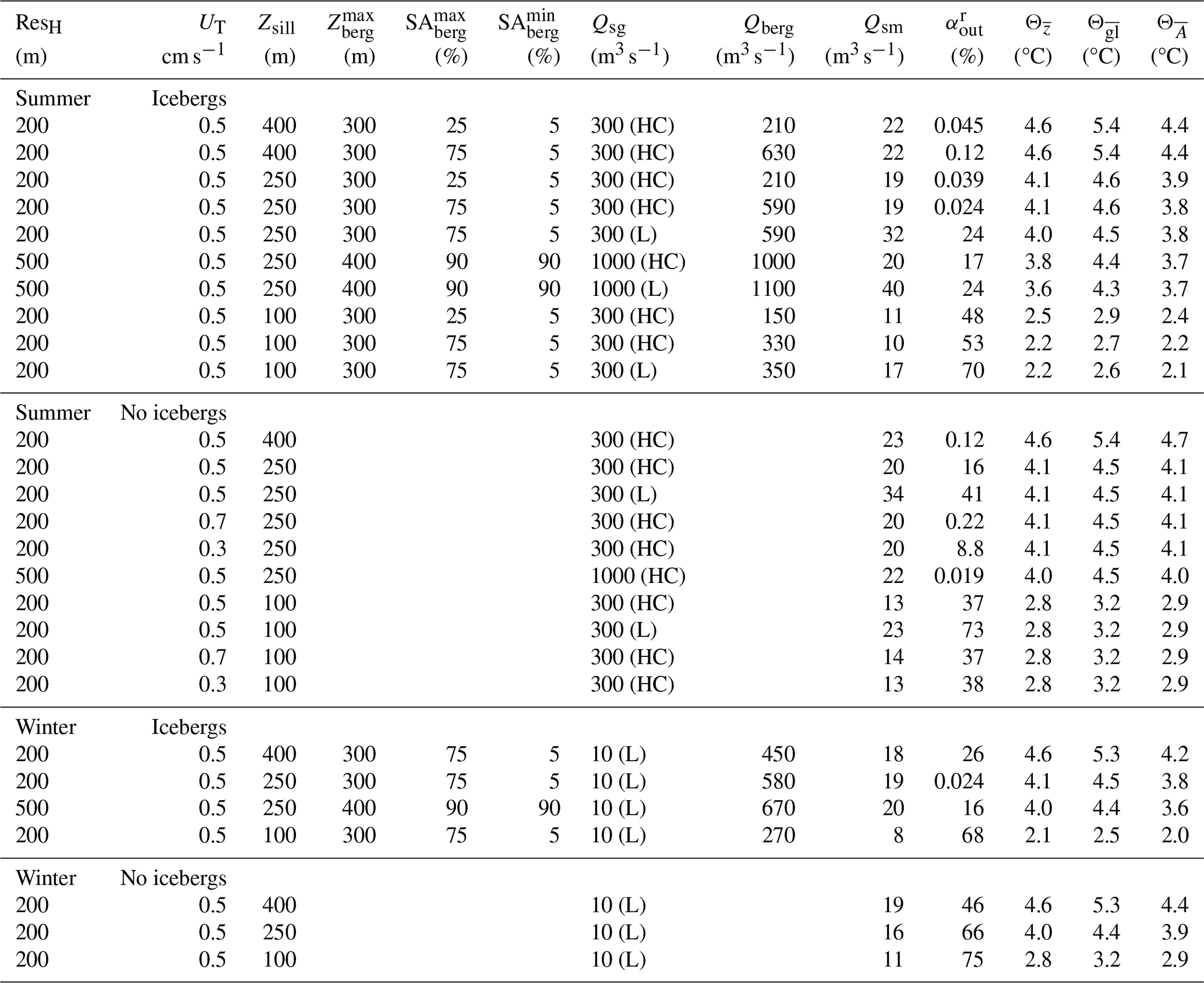
Table 1Forcing conditions and primary diagnostics for each simulation. For subglacial discharge, HC indicates a half-conical plume and L denotes a line plume.
2.1 Model setup
MITgcm fjord geometries were typical of Greenland fjords (e.g., Straneo and Cenedese, 2015) and were 800 m deep, 5 km wide, and 60 km long and had a laterally uniform, Gaussian-shaped sill near the mouth of the fjord with a minimum depth (Zsill) of either 100, 250, or 400 m (hereafter distinguished as S100, S250, and S400 runs; Fig. 1, Hager, 2023). We varied the sill depth because sills are dominant mechanisms for local water transformation within fjords (e.g., Ebbesmeyer and Barnes, 1980; Cokelet and Stewart, 1985; Hager et al., 2022; Bao and Moffat, 2024), while other geometric constraints, such as length and width, influence fjord circulation (e.g., Carroll et al., 2017) but are not expected to greatly alter fjord water properties. We did not include runs without sills because preliminary simulations showed no difference from S400 runs. The vertical resolution was 10 m in the upper 100 m, 20 m between 100–500 m depth, and 50 m below 500 m. The majority of runs had horizontal resolutions (Hres) of 200 m; however, a few high subglacial discharge and iceberg meltwater flux runs were conducted at 500 m resolution to avoid running at an impractical time step (Table 1). An 800 m deep coastal zone was constructed outside the fjord with an additional 30 cells to the west and 20 cells to the north and south. Hres in the coastal zone linearly telescoped to 2 km at the northern, western, and southern open boundaries. A 10-cell sponge layer was imposed at each open boundary to inhibit internal waves from reflecting back into the domain.
All simulations were run in a hydrostatic configuration with a nonlinear free surface and a Coriolis frequency of 1.3752 × 10⁻⁴ s−1. High- and low-resolution simulations were run at time steps of 25–30 and 60 s, respectively. The horizontal viscosity was prescribed using a Smagorinsky scheme (Smagorinsky, 1963) and a Smagorinsky constant of 2.2, while horizontal diffusivities were set to 0 (though numerical diffusion will still exist). We used the K-profile parameterization (KPP) (Large et al., 1994) for vertical mixing, setting the background and maximum viscosity to 5 × 10⁻⁴ and 5 × 10⁻³ s−1, respectively, and background and maximum diffusivities to 0 and 5 × 10⁻⁵ s−1, respectively. Simulations were run until all fjord water below the sill depth had been flushed and water properties stopped evolving (200–1000 d, depending on fjord flushing time). This step was necessary to ensure simulated fjords had time to fully respond to their unique forcing conditions and to remain consistent with the tacit steady-state assumption made in ISMIP6 thermal forcing parameterizations. The output was averaged over the last 10 d of model time to remove the influence of tides or internal waves, and all “near-glacier” model output was averaged over the two closest grid cells to the glacier face. “Grounding line” water properties are an average of the bottommost near-glacier cells. In total, we ran 27 simulations, each with differing combinations of sill depths, tidal velocities, subglacial discharge plume magnitudes and geometries, iceberg concentrations, and iceberg keel depths (Table 1).
Simulations were initialized from temperature and salinity data profiles observed in 2013–2015 outside the Uummannaq Fjord system, West Greenland (Bartholomaus et al., 2016), which shares a similar vertical structure to summer coastal properties around Greenland: a warm, fresh summer surface layer underlain by cold Polar Water and warm, salty Atlantic Water at depth (Fig. 1c; Straneo et al., 2012; Straneo and Cenedese, 2015). The same profiles were used as boundary conditions along the open boundaries (Fig. 1a). M2 frequency tidal velocities (UT) of 5 × 10⁻³ m s−1 were imposed along the western boundary, creating tidal amplitudes of ∼ 1.5 m within the fjord, typical of tides throughout East and West Greenland (Howard and Padman, 2021). In shallow-silled fjords (S100 and S250 simulations), where significant tidal mixing was plausible (e.g., Hager et al., 2022; Bao and Moffat, 2024), we tested additional high and low tidal forcing scenarios with UT values of 7 × 10⁻³ and 3 × 10⁻³ m s−1, creating tides of 2.06 and 0.88 m, respectively (Table 1).
Subglacial discharge (Qsg) and glacier submarine melting (Qsm) were parameterized with the IcePlume package (Cowton et al., 2015) using a straight glacier face along the eastern boundary (Fig. 1b, d). Summer high-resolution runs were forced with a subglacial discharge of 300 m3 s−1, which is typical of summer values from Kangilliup Sermia (Rink Isbræ) (Bartholomaus et al., 2016; Carroll et al., 2016). Summer low-resolution runs were designed to resemble the largest Greenland glacial fjords and were forced with a subglacial discharge of 1000 m3 s−1, characteristic of glacier runoff entering Sermilik Fjord and Kangiata Sullua (hereafter referring to Ilulissat Icefjord) (Echelmeyer and Harrison, 1990; Gladish et al., 2015; Carroll et al., 2016; Moon et al., 2018). Subglacial discharge plumes are parameterized to have a half-conical geometry in most runs; however, we test the influence of plume geometry (and thus near-terminus subglacial hydrology) by repeating five runs with subglacial discharge spread out across a 1 km wide line plume (Table 1; e.g., Jenkins, 2011), which may be more realistic for some fjord systems (Jackson et al., 2017; Hager et al., 2022; Kajanto et al., 2023). Winter scenarios were reinitialized from the steady state of summer runs with the same tidal, iceberg, and geometric constraints but were forced by a 10 m3 s−1 line plume across the entire glacier width (Table 1) to account for a switch to basal-friction-generated, distributed subglacial drainage in the winter (e.g., Cook et al., 2020). To be consistent with ISMIP6 methodology, we do not account for seasonal differences in offshore waters; thus, our seasonal sensitivity runs only test seasonal variation in subglacial discharge. In all runs, a background velocity of 0.1 m s−1 was applied along the glacier face to facilitate ambient submarine melting.
Icebergs were parameterized using the IceBerg package (Davison et al., 2020), which treats icebergs as stationary barriers to flow and adjusts surrounding fjord water properties according to calculated iceberg meltwater fluxes (Qberg). Iceberg depths were set using an inverse-power-law size frequency distribution with an exponent of −1.9, similar to those observed in Sermilik Fjord and Kangilleq – the fjord where Kangilliup Sermia terminates (Sulak et al., 2017). Consistent with observations (e.g., Enderlin et al., 2016; Sulak et al., 2017; Moon et al., 2018; Schild et al., 2021), we prescribed a maximum iceberg depth () of 300 and 400 m in high- and low-resolution runs, respectively (Fig. 1d). Icebergs were concentrated at the fjord head, covering a maximum surface area () of either 25 % or 75 % within 10 km of the glacier, which linearly decreased to a minimum surface area () of 5 % just inside the entrance sill (Fig. 1c). These concentrations approximate those observed at Kangilleq and Sermilik fjords (Sulak et al., 2017). Additional S250 simulations targeting the ice-choked conditions of Kangiata Sullua were conducted at low resolution using an iceberg concentration of 90 % throughout the fjord. Meltwater plumes resulting from iceberg submarine melt were parameterized by imposing a background velocity of 0.06 m s−1 along the iceberg face. All forcing and geometric conditions (except tidal sensitivity experiments) were repeated with and without icebergs. We did not include sea ice formation in our simulations and do not expect the neglect of associated latent heating and brine rejection to significantly affect our results, particularly in deep fjords. However, it is possible sea ice formation could influence thermal forcing in some shallow fjords.
2.2 Testing of ISMIP6 thermal forcing parameterizations
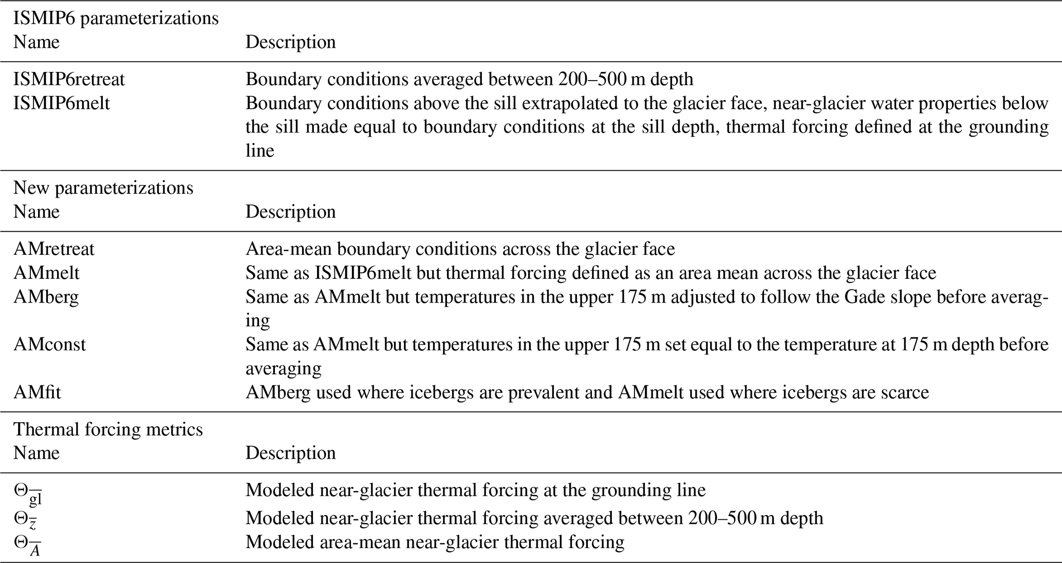
For comparison to our simulations, we calculate the thermal forcing that would have been imposed in ISMIP6 experiments assuming regional water properties equal to our open boundary conditions. In the first thermal forcing parameterization (ISMIP6retreat; Table 2) used with Eq. (1), thermal forcing is determined by
where θ and S are the profiles of prescribed potential temperature and practical salinity at the open boundaries; θf is the local freezing temperature at depth z; and λ1 = −5.73 × 10⁻² °C psu−1 (practical salinity unit), λ2 = 8.32 × 10⁻² °C, and λ3 = 7.61 × 10⁻⁴ °C m−1 (Jenkins, 2011). Profiles of Θ(z) are then depth-averaged between 200–500 m depth (Slater et al., 2020) to provide a singular value, = 4.7 °C (Table 2), across all simulations for ISMIP6retreat. This range of depth was chosen to encompass most Greenland tidewater glacier grounding lines (Slater et al., 2019).
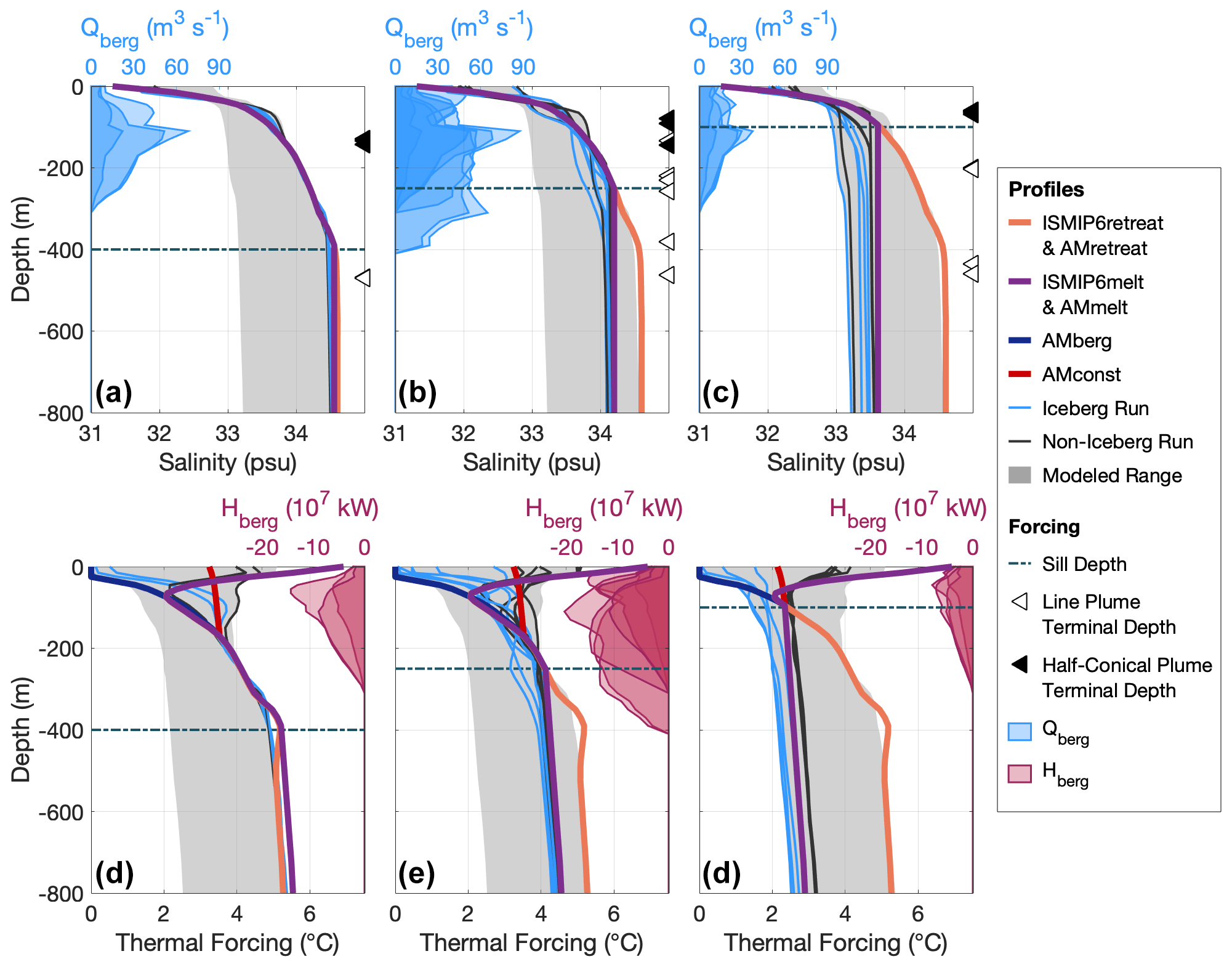
Figure 2Near-glacier (a–c) salinity and (d–f) thermal forcing profiles for all iceberg (light blue) and non-iceberg (gray) runs (a and d are S400 runs, b and e are S250 runs, c and f are S100 runs). Also plotted are the profiles used to calculate ISMIP6retreat and AMretreat (orange), ISMIP6melt and AMmelt (purple), AMberg (blue; Sect. 4.2), and AMconst (red; Sect. 4.2). The orange profile is also equivalent to the boundary conditions. The gray background in all plots illustrates the range across all runs, and the horizontal dashed line depicts the sill depth. Triangles in (a–c) represent the terminal plume depth for line plumes (white) and half-conical plumes (black). The vertical distributions of iceberg freshwater fluxes (Qberg) and heat fluxes (Hberg) are shown in (a)–(c) and (d)–(f), respectively, to depict the depth of iceberg melt relative to the sill depth and profile variability.
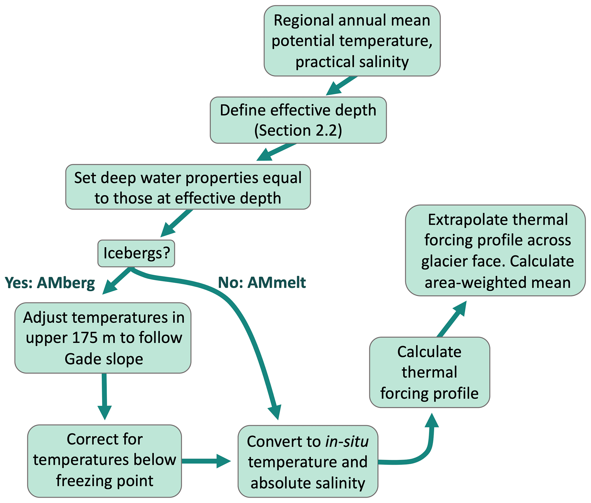
In contrast to ISMIP6retreat, the submarine melt thermal forcing parameterization (ISMIP6melt) accounts for bathymetry preventing external water from entering the fjord below the sill depth (Table 2; Morlighem et al., 2019). This is accomplished by first defining an effective depth as the deepest part of the near-glacier water column in direct contact with the open ocean (here equal to the sill depth). Fjord water properties above the effective depth are directly extrapolated to the glacier terminus, while water properties below the sill depth are made equal to those at the effective depth (e.g., Morlighem et al., 2019). Extrapolated potential temperature and practical salinity are then converted to in situ temperature and absolute salinity before calculating thermal forcing across the glacier face: Θ(z) = T(z)−Tf(z). Here, T and Tf are the in situ temperature and freezing temperature, which together with the absolute salinity are calculated using the non-linear TEOS-10 toolbox (McDougall and Barker, 2011). As in Slater et al. (2020), the final Θ value used in Eq. (2) is taken from the grounding line depth. The ISMIP6melt formulation therefore predicts the same grounding line thermal forcing () for all runs within each of the S100 (2.9 °C), S250 (4.6 °C), and S400 (5.5 °C) groups (Fig. 2).
Although methods differ, both ISMIP6 parameterizations are designed to at least crudely target thermal forcing at glacier grounding lines for two reasons: (1) buoyant upwelling along the glacier terminus may homogenize the near-glacier water column (e.g., Mankoff et al., 2016), and (2) grounding line thermal forcing may promote undercutting, and thus calving, of the glacier face. To remain consistent with their original formulations, we test each parameterization against our simulations by comparing it to its own intended metric of thermal forcing near the grounding line. ISMIP6retreat is thus compared to , the modeled near-glacier thermal forcing averaged between 200–500 m depth, while ISMIP6melt is compared to , the modeled near-glacier thermal forcing at the grounding line. Later, a third thermal forcing metric, , the modeled area-mean (vertically and horizontally averaged) near-glacier thermal forcing, is used to test additional parameterizations (Table 2).
We use root mean square errors (RMSEs) to compare like values between parameterizations and model runs. However, the best depth at which to prescribe thermal forcing at a calving face is still a topic of ongoing debate (see Sect. 4.1). We therefore also employ a Willmott skill score (Willmott, 1981) to assess each parameterization's ability to predict thermal forcing throughout the entire water column. The Willmott skill score (SS) is defined as
where mi is the MITgcm or observed near-glacier thermal forcing at z coordinate i, is the mean of all mi values, pi is the corresponding value predicted by each parameterization, and N is the number of z coordinates in a profile. An SS value of 1 indicates perfect agreement, while a value of 0 indicates no agreement between profiles.
Table 2Descriptions of ISMIP6 thermal forcing parameterizations, new thermal forcing parameterizations presented in this paper (see Sect. 4.2), and thermal forcing metrics extracted from our simulations.
2.3 Quantification of sill-driven mixing
Sill-driven mixing is a primary control on circulation and water properties in shallow-silled glacial fjords in Alaska and Patagonia (Hager et al., 2022; Bao and Moffat, 2024) and may additionally influence near-glacier thermal forcing in Greenland. Following MacCready et al. (2021), Hager et al. (2022), and Bao and Moffat (2024) we quantify the net effect of sill-driven vertical mixing by pairing the estuarine total exchange flow (TEF) framework (MacCready, 2011) with efflux–reflux theory (Cokelet and Stewart, 1985). We use this approach because it provides bulk mixing transports that are easily relatable to other forcing processes. TEF utilizes isohaline coordinates to identify inflowing and outflowing transports that satisfy the Knudsen relations and account for both tidal and subtidal fluxes (Knudsen, 1900; MacCready, 2011; Burchard et al., 2018). We use 1000 salinity classes to bin salt and volume fluxes across each transect and employ the dividing salinity method (MacCready et al., 2018; Lorenz et al., 2019) to calculate inward and outward transports, allowing for the potential for multiple layers of each to exist. Inflowing and outflowing transport-weighted salinities are given by , where and Qin,out are the sums of all inflowing and outflowing salt and volume fluxes, respectively. We treat temperature as a tracer corresponding to each salt class so that the transport-weighted inflowing and outflowing temperatures are calculated as (e.g., Lorenz et al., 2019).
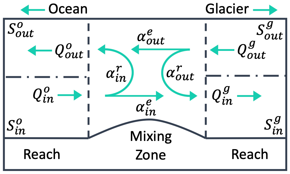
Efflux–reflux theory assumes an estuarine system where mixing is concentrated at constrictions (such as sills) separated by deep basins (dubbed reaches) where mixing is minimal (Cokelet and Stewart, 1985). At each mixing zone, some portion of inflowing or outflowing water is vertically mixed and recirculated, or refluxed, into the opposing layer and back into its original reach, while the remainder, the efflux, is transported across the mixing zone to the next reach (Fig. A1). Using mass and volume conservation, the percentage of inflowing or outflowing water that is refluxed or effluxed can be written in terms of TEF variables (MacCready et al., 2021), but for the purposes of this paper, we are primarily concerned with , which represents the percent of the outflowing fjord water that is refluxed at the entrance sill:
where superscripts o and g denote the TEF transports on the oceanward and glacierward sides of the mixing zone, respectively (Fig. A1). We calculated efflux–reflux budgets between two TEF transects on either side of the entrance sill and avoid prescribing icebergs within the sill region to ensure temperature and salt are conserved across the mixing zone. More information about using TEF with efflux–reflux theory can be found in MacCready et al. (2021), Hager et al. (2022), and Appendix A.
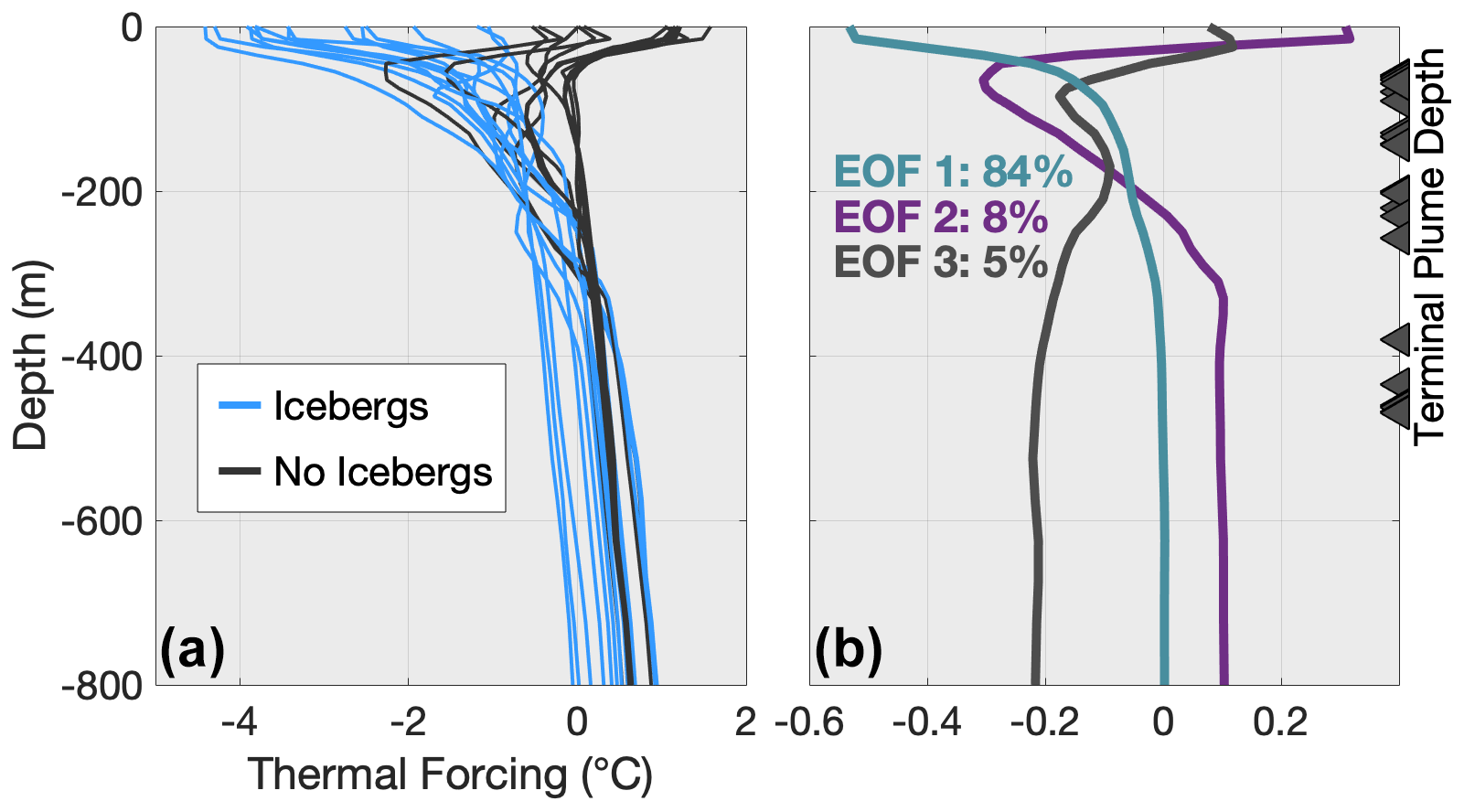
Figure 3(a) Near-glacier thermal forcing profiles from all iceberg (light blue) and non-iceberg (gray) runs after removing the depth average of each sill group. (b) The three dominant EOF modes with the percentage of variance they contribute, as calculated from the profiles in (a). Gray triangles indicate terminal plume depths of all runs. The teal line represents variance from iceberg melting, the purple line indicates variance stemming from the boundary conditions, and the gray line signifies variance from subglacial discharge plumes.
2.4 Calculation of local heat fluxes
Quantifying the heat fluxes associated with each local forcing mechanism is important when determining the primary causes of local water transformation. The heat flux resulting from the submarine melting of ice (Hmelt) is calculated by
where ρmw is the meltwater density (1000 kg m−3), Qmw is the total meltwater flux as determined from IceBerg or IcePlume, L is the latent heat of fusion, ci is the heat capacity of ice, θf is the potential freezing temperature, and θi is the potential temperature of ice. In our experiments, ice is set to its melting temperature so that Eq. (6) collapses to
and
for the iceberg and glacier submarine melt heat fluxes, respectively.
Advective heat fluxes (Hadv) arising from sill-driven reflux and subglacial discharge are given by
where ρ is the water density, cp is the heat capacity of water, Q is the advective volume flux, θadv is the potential temperature of the advected fluid, and θr is a reference temperature. To calculate the recirculatory heat flux caused by sill-driven mixing (here called heat reflux), we substitute TEF quantities into Eq. (9) so that
where is the reflux volume; is the temperature difference between the outflowing and inflowing layers on the sill's glacierward side; and ρ is the refluxed water density as determined from , , and the mid-column water pressure at 400 m depth. Here, Hreflux refers to the heat transfer (positive or negative) from the outflowing layers to inflowing layers on the sill's glacierward side as a result of sill-driven mixing. For the subglacial discharge heat flux, Eq. (9) is specified as
where Qsg is the total subglacial discharge; ρsg is 1000 kg m−3; Tsg is 0 °C; and the reference temperature, , is chosen to be consistent with Eq. (10). In practice, works well as a reference temperature in both Eqs. (10) and (11) as inflowing water properties remain largely unaltered between the sill and glacier face.
2.5 Empirical orthogonal functions of near-glacier variability
Empirical orthogonal function (EOF) analysis was conducted on near-glacier thermal forcing profiles to determine the dominant modes of variability between runs. Near-glacier Θ(z) profiles were horizontally averaged across the calving face before removing the mean Θ within each sill group (Fig. 3a). This second step was necessary to account for the dependence of mean fjord temperatures on the sill depth (Fig. 2). EOFs were then calculated on the resultant profiles.
3.1 Near-glacier water properties
Despite identical temperature and salinity forcing at the open boundaries, varied by 2.7 °C across all runs (Table 1). varied by 2.9 °C between runs, while grounding line salinities differed by 1.4 psu (Fig. 2, Table 1). In S400 runs, near-glacier water properties were largely unmodified from the open boundary conditions, particularly below 200 m, where the influence of subglacial discharge and iceberg melt was negligible (Fig. 2). However, water properties below the sill depth progressively freshened and cooled as the sill depth shoaled, allowing for to be neatly grouped by depth of sill: 4.2–4.7 °C for S400 runs, 3.6–4.1 °C for S250 runs, and 2.0–2.9 °C for S100 runs (Fig. 2, Table 1).
Water properties below the sill depth were nearly homogeneous in all runs, with only minor variability occurring when iceberg keels extended below the sill depth (see Qberg and Hberg in Fig. 2) or subglacial discharge plumes reached neutral buoyancy below the sill depth (this most often occurs with line plumes; see black and white triangles in Fig. 2a-c). The greatest variability existed above 175 m, where most iceberg melting occurred and where most summer subglacial discharge plumes reached neutral buoyancy (Fig. 2). Horizontal gradients in water properties were concentrated over the sill region and were negligible within the fjord (Hager, 2023).
Unsurprisingly, iceberg runs were always cooler than their non-iceberg counterparts; however, the difference between these groups was larger for runs with shallower sills (Table 1, Fig. 2). On average, the difference in between iceberg and non-iceberg runs diminished from 0.7 °C for S100 runs to 0.3 and 0.2 °C for S250 and S400 runs, respectively. Iceberg melt had the greatest impact on water properties in the upper 175 m, contributing to a temperature range of 5.1 °C at the surface, independent of the sill depth (Fig. 2). However, where iceberg keel depth exceeded the sill depth, iceberg melting cooled the entire water column to the grounding line (Fig. 2), indicating some volume of iceberg meltwater was mixed and refluxed at the silled mixing zone. Such cooling is most pronounced in S100 runs, where the difference in grounding line thermal forcing was on average 0.5 °C between iceberg and non-iceberg runs (Fig. 2). showed no significant difference between tidal sensitivity runs, nor was there an appreciable distinction between runs with line and half-conical plumes and otherwise equivalent forcing. Winter runs were generally cooler than their summer counterparts in the upper water column, with varying by ≤ 0.3 °C between winter and summer discharge scenarios with otherwise equivalent forcing (Table 1).
After removing the dominant influence of sills (Fig. 3a), EOF analysis indicates the presence or absence of icebergs accounts for 84 % of the remaining near-glacier thermal forcing variability between runs (Fig. 3b). In general, this first EOF mode reflects the same pattern of cooling in the upper 300 m present in all iceberg runs, but its amplitude changes sign for non-iceberg runs, thus imitating the warm surface water that exists when icebergs are absent (Fig. 3). The second EOF mode makes up 8 % of the variance between runs and has a spatial structure identical to the open boundary temperature conditions (Fig. 3b). Therefore, the second mode can be interpreted as the influence of regional ocean temperatures on near-glacier thermal forcing, in large part accounting for the minimal fjord water mass transformation in S400 non-iceberg runs. A physical interpretation of the third EOF mode, contributing 5 % of the variance, is less certain; however, this mode depicts temperature variability coincident with the terminal depths of subglacial discharge plumes (Fig. 3b) that is not easily relatable to any other forcing mechanism. We thus interpret the third EOF mode to represent variable outflowing plume conditions. As reflux primarily affects the water column below the sill depth, which is homogeneous and similar to depth-averaged water properties, variability resulting from reflux was likely removed with the depth average when computing EOFs. It is therefore possible that reflux variability is incorporated into any of the three dominant modes, part of the remaining 3 % of the variance without clear physical corollaries was removed with the mean during EOF computation.
3.2 Internal freshwater sources and heat fluxes
Subglacial discharge and iceberg meltwater had similar contributions (∼ 30 %–65 %) to the total freshwater input into summer iceberg runs, with glacial meltwater contributing less than 4 % (Table 1). In contrast, iceberg melt flux was the dominant freshwater source (∼ 95 % of all freshwater fluxes) in winter iceberg runs. In non-iceberg runs, subglacial discharge made up ≥ 90 % of freshwater input in the summer, while glacier submarine melt was the dominant freshwater source in the winter (53 %–65 % of all freshwater fluxes; Table 1).
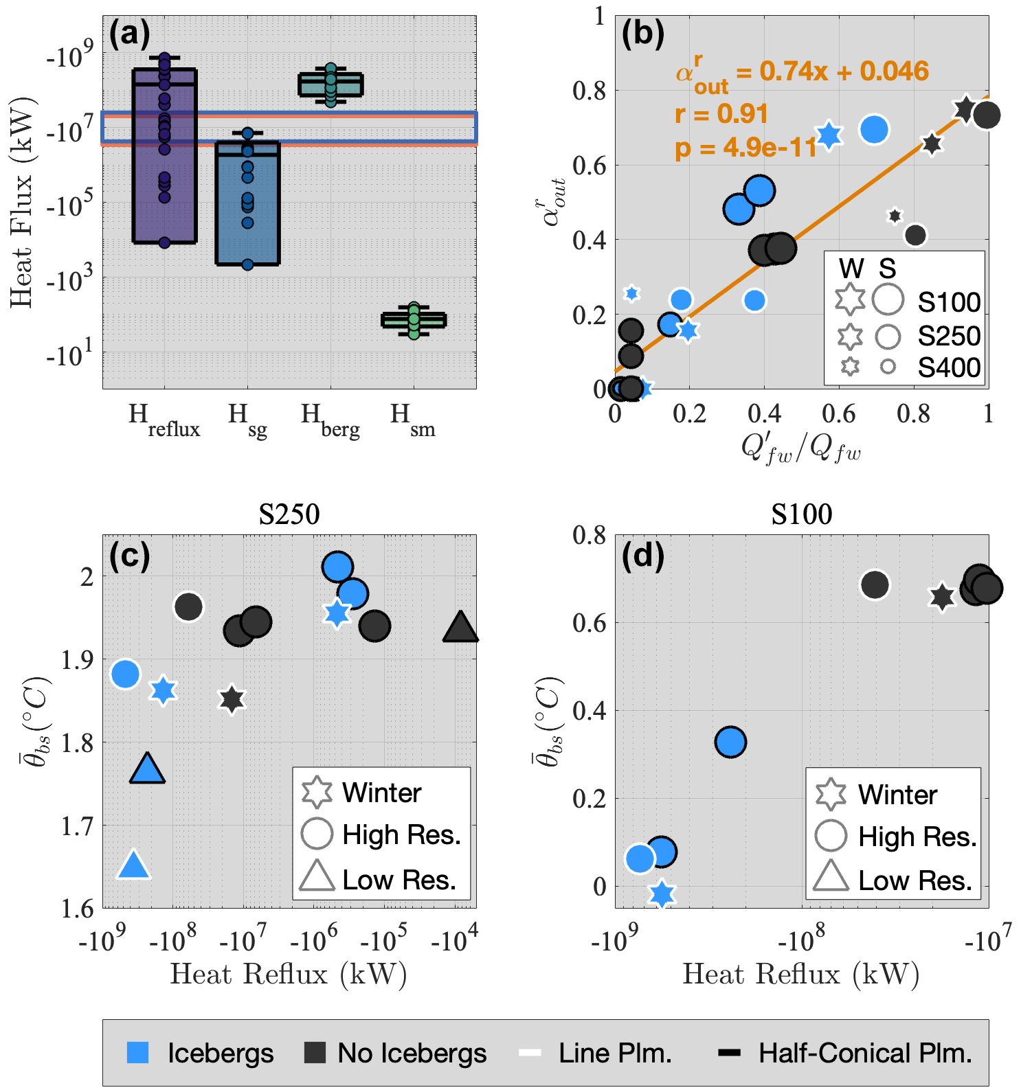
Figure 4(a) Box plots of heat fluxes associated with reflux (Hreflux), subglacial discharge (Hsg), iceberg submarine melting (Hberg), and glacier submarine melting (Hsm). Box plots depict the maximum, minimum, mean, and standard deviation across all runs. Horizontal blue and orange rectangles depict ranges of estimated surface heat fluxes (Sect. 4.1) for winter and summer runs, respectively. Note that summer surface heat fluxes are reflected across the x axis for illustrative purposes but are actually positive and represent surface warming. (b) Reflux fraction () as a function of , which is the portion of freshwater input released below the sill depth. Stars and circles differentiate between winter and summer runs, respectively. Marker sizes vary by the sill depth. Orange line is Eq. (12). (c–d) Depth-averaged near-glacier potential temperatures below the sill depth () as a function of heat reflux for the S250 and S100 runs. Marker shape differentiates between winter (stars), summer high-resolution (circles), and summer low-resolution (triangles) runs. In (b)–(d), light-blue and gray markers represent iceberg and non-iceberg runs, respectively, and white edges depict runs forced with a line plume.
Despite comparable freshwater fluxes in summer runs, the heat flux from iceberg submarine melting surpassed that from subglacial discharge by multiple orders of magnitude, regardless of iceberg concentration or subglacial discharge (Fig. 4a). Iceberg melting removed heat from surrounding waters at rates of −4.9 × 10⁷ to −3.8 × 10⁸ kW. In contrast, subglacial discharge heat fluxes were −2.2 × 10³ to −7.2 × 10⁶ kW and glacier submarine melt heat fluxes were −29 to −150 kW. Heat reflux spanned 5 orders of magnitude from −8.3 × 10³ to −7.4 × 10⁸ kW, at its maximum exceeding the magnitudes of even the largest iceberg heat fluxes, while at its minimum falling near the lower limits of subglacial discharge heat flux.
As opposed to heat fluxes from freshwater sources, which principally cool the upper water column, heat reflux can directly facilitate the cooling of deep water. Our experiments show a pronounced cooling of deep-water temperatures with increasingly negative heat reflux for both S250 and S100 runs, resulting in a decrease of over ∼ 0.3 and ∼ 0.6 °C, respectively (Fig. 4c–d). In general, the runs with the highest heat reflux contained either icebergs, line plumes, or both; however, there is no clear relationship between heat reflux and any specific local forcing processes (Fig. 4a–b). Nevertheless, there is a highly significant (r=0.91, p = 4.9 × 10⁻¹¹) linear relationship between the portion of freshwater input released below the sill depth and the percent of outflowing water refluxed at the entrance sill, (Fig. 4b). In our experiments, can be estimated by
where is the total freshwater input and the prime denotes freshwater entering the domain below the sill depth (subglacial discharge is included in if the plume reaches neutral buoyancy below the sill depth).
All S100 runs had significant sill-driven reflux ( 37 %). in S250 runs ranges from 0 %–66 % but is highest in runs with substantial iceberg freshwater flux below the sill depth or in runs with line plumes (Fig. 4b). was negligible in all summer S400 runs but became significant in winter runs where weak subglacial discharge plumes still intersected the sill at depth (Table 1). Despite an equivalent between S100 tidal sensitivity runs (∼ 37 %), tidal forcing does have a minor effect on S250 runs and is responsible for a range of 0.2 %–16 % in across S250 tidal scenarios (Table 1).
Table 3RMSE and skill score of thermal forcing parameterizations for different groups of model runs. The RMSE of ISMIP6melt is calculated relative to , while the RMSE of ISMIP6retreat is calculated relative to . The RMSE of all other parameterizations is relative to . Bold values indicate the most accurate parameterization for each group of runs.
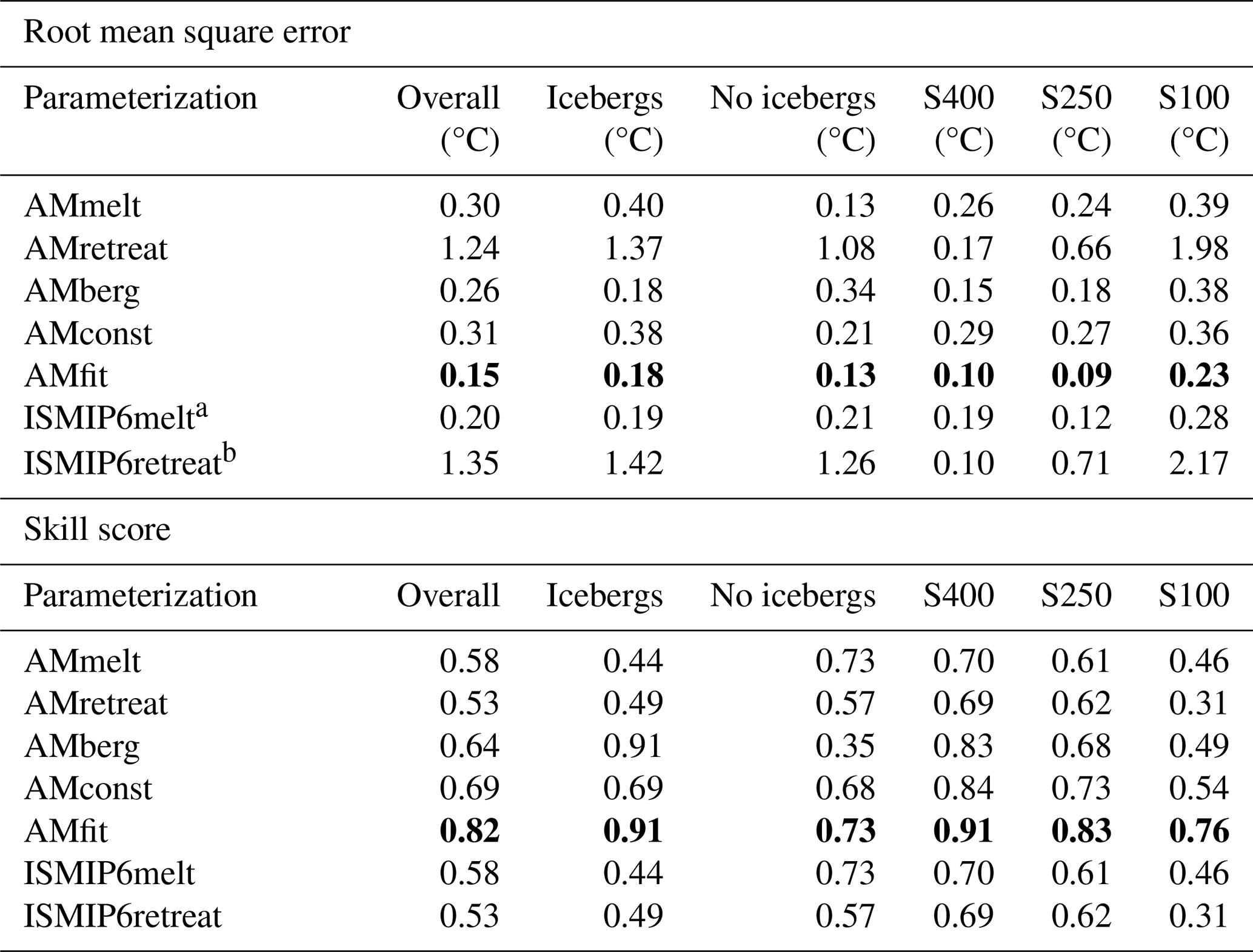
a RMSE is calculated relative to . b RMSE is calculated relative to .
3.3 Thermal forcing parameterizations
Overall, ISMIP6melt accurately predicted within an RMSE of 0.2 °C, an error that varied by ± 0.08 °C regardless of the sill depth or iceberg prevalence (Table 3). ISMIP6retreat predicted mean near-glacier thermal forcing between 200–500 m depth () within an RMSE of 1.35 °C (Table 3). This error was minimal (RMSE = 0.10 °C) for S400 runs, in which fjord water was of similar composition to shelf water but increased substantially with successively shallower sills (RMSE = 0.71 °C for S250 runs and RMSE = 2.17 °C for S100 runs; Table 3). Both profiles used to compute ISMIP6melt and ISMIP6retreat had moderate success at parameterizing the near-glacier thermal forcing profile, with average skill scores of 0.5–0.6 across all runs (Table 3). Skill scores for iceberg runs were relatively poor (SS = 0.44–0.49) compared to non-iceberg runs (SS = 0.57–0.73). Skill scores also steadily decreased with the sill depth from ∼ 0.70 in S400 runs to 0.31–0.46 in S100 runs (Table 3).
4.1 Uncertainty in thermal forcing parameterizations
Our results demonstrate the wide range of fjord conditions that can result from equivalent regional ocean forcing and emphasize the need for local processes to be incorporated into the coupling of global climate and ice sheet models. We assign importance to each local forcing mechanism based on its impact on near-glacier thermal forcing, which we corroborate with additional evidence where possible. In order of importance, we identify the dominant local forcing mechanisms as the following.
-
Bathymetric obstruction of external water. The 2.7 °C range in in our runs is strongly dependent on the depth of the entrance sill, which preferentially blocks warm water from entering the fjord when the sill is shallow. The prominent thermocline between 100–400 m depth in our boundary conditions (Fig. 1c) has been observed in fjords throughout Greenland and marks the transition between Polar Water and Atlantic Water (Straneo et al., 2012). In our experiments, external temperatures range from 0.46 °C at 100 m to 3 °C at 400 m depth (Fig. 1c), nearly the exact range in between S100 runs and S400. Furthermore, we see no overlap in between the three sill depths. Therefore, we conclude that the depth of the entrance sill in relation to the 100–400 m thermocline plays a first-order role in determining internal fjord temperatures, but we do not expect the sill depth to be a strong control when sills lie below the Polar Water–Atlantic Water thermocline.
-
Presence or absence of icebergs. After adjusting for the silled obstruction of external water, cooling from iceberg meltwater (or lack thereof) is responsible for 84 % of the remaining variability between runs (Fig. 3), as well as a temperature difference of 5.1 °C at the surface. Iceberg-driven cooling primarily occurs in the upper 175 m of the water column; however, where iceberg keels extend below the sill depth, cooling affects the entire water column as a result of sill-driven reflux. Similar magnitudes of iceberg-driven cooling were modeled in Davison et al. (2020), Davison et al. (2022), and Kajanto et al. (2023). Iceberg meltwater fluxes are comparable to subglacial discharge in summer runs and dominate the freshwater budget in the winter, which is in agreement with prior estimates of iceberg meltwater fluxes in Greenland fjords (Enderlin et al., 2016; Moon et al., 2018). However, the additional energy required to melt this volume of water enables icebergs to disproportionately cool the surrounding water column when compared to a similar volume flux of subglacial discharge.
-
Refluxed outflowing water. Heat reflux can rival the heat flux of iceberg melting, leading to a substantial cooling of deep-water temperatures. Where heat reflux is important, the ≲ 0.6 °C cooling occurs throughout the water column from the sill depth to the grounding line, often affecting a much larger portion of the water column than the melting of icebergs. While such an effect is hard to identify with EOF analysis, the decrease in deep-water temperatures with heat reflux (Fig. 4c and d) indicates this process has the potential to significantly impact near-glacier thermal forcing in certain fjords.
-
Subglacial discharge. While subglacial discharge certainly affects near-glacier thermal forcing, its contribution to variability in near-glacier thermal forcing (both inter- and intra-seasonal) is overshadowed by the influence of icebergs. EOF analysis suggests subglacial discharge is responsible for only 5 % of the near-glacier temperature variability. However, subglacial discharge remains a critical driver of submarine melting through its influence on glacial fjord circulation (Carroll et al., 2015; Sciascia et al., 2013; Straneo et al., 2011; Xu et al., 2012), deep-water renewal (Carroll et al., 2017), turbulent upwelling (Slater et al., 2015), near-glacier horizontal circulation (Slater et al., 2018), and enhanced iceberg melt (Kajanto et al., 2023). Our results further indicate the terminal depth of subglacial discharge plumes can directly affect reflux at silled mixing zones (Fig. 4b) and thus influence deep-water temperatures.
-
Surface heat flux. Although we neglect surface heat fluxes in our model, we approximate their magnitude based on previous estimates from Sermilik Fjord. Surface heat fluxes in Sermilik Fjord are thought to be ∼ 80 W m−2 in the summer and ∼ −100 W m−2 in the winter (Jackson and Straneo, 2016; Hasholt et al., 2004). Applying these values to the exposed surface area (not covered by icebergs) in our simulations, we estimate total surface heat fluxes in our simulations would be 3.4 × 10⁶ to 2.0 × 10⁷ kW in the summer and −4.3 × 10⁶ to −2.5 × 10⁷ kW in the winter (Fig. 4a). Thus, surface heat fluxes could often exceed those from subglacial discharge but are an order of magnitude less than iceberg melt heat fluxes. However, surface heating only affects the uppermost water column, and thus we do not expect it to substantially affect in Greenland fjords. Nevertheless, surface heating may significantly affect heat reflux in Alaska, Svalbard, and Patagonia fjords where shallow sills protrude into the surface layer (e.g., Hager et al., 2022; Bao and Moffat, 2024).
-
Glacier submarine melting. While our modeling suggests glacier submarine melting has little effect on near-glacier thermal forcing, we cannot discount it as an important variable. Our model resolution is too coarse to resolve the complexities of the ice–ocean boundary, and recent observations indicate the IcePlume package may substantially underestimate ambient melting (Jackson et al., 2020).
Observational studies support these model-identified drivers of contrasting water properties between nearby fjords. In northwestern Greenland, slight differences in sill geometry allow for warm Atlantic Water to flow unimpeded into Petermann Fjord, while the inflow of Atlantic Water into the inner basin of neighboring Sherard Osborn Fjord is restricted to a cross-sectional area ∼ 7.5× smaller (Jakobsson et al., 2020). When paired with enhanced sill-driven reflux of glacially modified water, this restricted heat inflow is responsible for a 0.2 °C difference in near-glacier water between these otherwise similar fjords (Jakobsson et al., 2020). Furthermore, Kangilliup Sermia, Kangerlussuup Sermia, and Sermeq Kujalleq (hereafter referring to Jakobshavn Isbræ) are all located within the same ISMIP6 region and are thus subject to the equivalent ocean thermal forcing in ISMIP6 projections (except for bathymetric adjustments used for ISMIP6melt) (Slater et al., 2020). Yet, mean fjord temperatures in the upper 100 m differed by up to 2.5 °C in summer 2014, seemingly due to the large iceberg meltwater flux into Kangiata Sullua, where Sermeq Kujalleq terminates (Bartholomaus et al., 2016; Mojica et al., 2021; Kajanto et al., 2023).
In addition to local forcing processes, our results point to a further source of error in the commonly used thermal forcing parameterizations, namely that current parameterizations only define thermal forcing at specific depths (e.g., at the grounding line or between 200–500 m). For ISMIP6retreat, a depth average of regional ocean thermal forcing from 200–500 m was chosen to encompass most Greenland tidewater glacier grounding lines (Slater et al., 2020), yet this depth range also bounds the largest vertical temperature gradient along the Greenland coast. Thus, any sill that exists within or above this range will greatly affect the ability of ISMIP6retreat to accurately predict near-glacier thermal forcing. Indeed, ISMIP6retreat was quite accurate for S400 runs, in which the difference in 200–500 m temperatures between external and internal water was minimal, but its accuracy decreased progressively with each shallower sill as the temperature difference between external and internal water increased to > 1.5 °C.
The current state of frontal ablation laws used in large-scale ice sheet models requires a single scalar to represent thermal forcing across the entire glacier terminus (e.g., Aschwanden et al., 2019; Choi et al., 2021). Unfortunately, this makes it difficult to define the best metric for prescribing near-glacier thermal forcing. Current methods often rely on grounding line conditions, motivated by the fact that grounding line submarine melt may promote undercutting and calving (e.g., Rignot et al., 2016; O'Leary and Christoffersen, 2013); however, glacier termini can actually exhibit a wide range of geometries resulting from spatially variable melt rates (Fried et al., 2019), which can either increase or decrease calving depending on the magnitude and shape of the entire melt profile (Ma and Bassis, 2019). Thus, an overemphasis on undercutting processes may lead to spurious frontal ablation laws. Furthermore, the choice to prioritize grounding line thermal forcing in both ISMIP6melt and ISMIP6retreat negates the iceberg-driven cooling of the upper water column, which our modeling indicates is the secondary control on near-glacier thermal forcing. While buoyant upwelling may partially homogenize near-terminus waters (at a finer scale than our model resolution), particularly within the subglacial discharge plume (e.g., Mankoff et al., 2016), it seems likely that iceberg meltwater remains an important control on thermal forcing at the ice–ocean boundary. Although it remains unclear at what depth glacier dynamics are most sensitive to ocean thermal forcing, from an ocean forcing perspective, it may be prudent to define thermal forcing using a metric that captures all processes relevant to near-glacier conditions, such as iceberg melting. Such an approach would also pave the way for coupled mélange–ice dynamics models, which would require an accurate portrayal of the upper water column to appropriately model mélange dynamics and prescribe back stress to the glacier. Therefore, we here test alternative methods for parameterizing a full profile of ocean thermal forcing, as well as an area mean, which allow for the inclusion of all dominant fjord-scale processes, while remaining relevant to calving processes.
4.2 Alternative thermal forcing parameterizations
We first test revisions to ISMIP6melt and ISMIP6retreat that are independent of specific depths, here called area-mean melt (AMmelt) and area-mean retreat (AMretreat), respectively (Table 2). Thermal forcing profiles are calculated as was done for ISMIP6melt and ISMIP6retreat, but they are extrapolated across the glacier terminus, with an area-mean thermal forcing being calculated instead of pulling from a set depth (Fig. C1). A third parameterization (AMberg) accounts for bathymetric obstructions in the same way as ISMIP6melt, but the surface 175 m follows the Gade slope submarine melt mixing line (Gade, 1979; Straneo and Cenedese, 2015) to approximate the influence of iceberg submarine melting on the upper water column (Fig. 2). For ice at the freezing temperature, the Gade slope is
As surface salinity in the fjord remains relatively similar to external water (Fig. 2), we leave salinity unchanged from ISMIP6melt and adjust temperatures accordingly to fit the Gade slope (Table 2). A final modification is made in which waters below freezing temperature are set to the in situ freezing point (Fig. C1). In practice, AMberg approximates a lower limit of cooling that occurs through iceberg melting, while AMmelt sets the upper bound on surface temperatures attainable for non-iceberg runs (Fig. 2). Therefore, we test a fourth, middle-ground parameterization (AMconst) in which the ISMIP6melt temperature and salinity at 175 m is extrapolated to the surface before calculating the thermal forcing profile (Fig. 2; Table 2). For both AMconst and AMberg, the final thermal forcing value used in Eqs. (1) and (2) is again an area mean across the glacier face.
The profiles used to calculate AMmelt and AMretreat each had a skill score of ∼ 0.55 and predicted within an RMSE of 0.30 and 1.24 °C, respectively; however, the RMSE of AMretreat remained heavily dependent on the sill depth (Table 3). As expected, AMmelt was a strong predictor of near-glacier thermal forcing in non-iceberg runs (RMSE = 0.13 °C; SS = 0.73), while AMberg performed well in iceberg runs (RMSE = 0.19 °C; SS = 0.91). AMconst was an adequate compromise between AMberg and AMmelt, with an RMSE of 0.31 °C and a skill score of 0.69 across the entire model ensemble (Table 3). Skill scores for all parameterizations decreased considerably with successively shallower sills (Table 3).
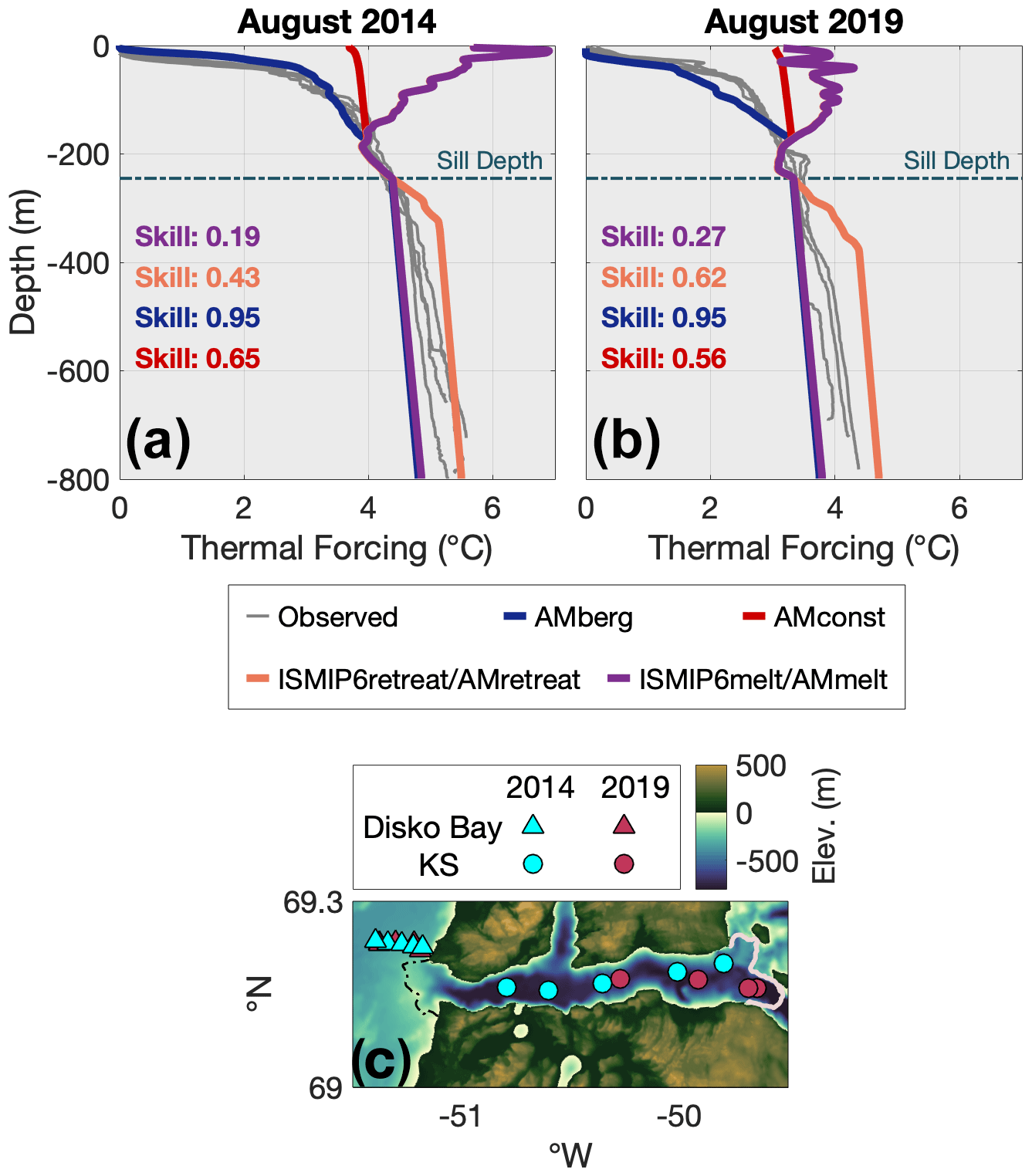
Figure 5Thermal forcing profiles (gray) observed within Kangiata Sullua (KS) via XCTD casts in (a) August 2014 and (b) August 2019, plotted with the profiles used to calculate ISMIP6retreat (orange) and AMberg (dark blue). The ISMIP6retreat profile is equivalent to external forcing conditions in Disko Bay. Skill score for each parameterization profile is also provided. Horizontal dashed line signifies the maximum depth (245 m) of the Kangiata Sullua entrance sill. (c) Bathymetric map rendering the locations of XCTD casts within Kangiata Sullua (circles) used in (a) and (b), as well as XCTD and CTD casts in Disko Bay (triangles) used to provide external forcing conditions. Solid rose line depicts the Sermeq Kujalleq terminus position in July 2014 (Goliber et al., 2022), and the dashed black line outlines the location of the entrance sill.
Encouraged by our model results, we test the efficacy of AMberg with observations using conductivity, temperature, and depth profiles collected by ship (CTD) and helicopter (XCTD, expandable) within Kangiata Sullua and the adjacent Disko Bay in August 2014 (Beaird et al., 2017) and August 2019 (Fig. 5; Appendix B). Temperature and salinity data from Disko Bay were used to calculate an average external thermal forcing profile analogous to ISMIP6retreat. Following the steps outlined above, a profile of AMberg was then constructed based on average Disko Bay temperature and salinity profiles. In both years, AMberg reproduced XCTD casts within Kangiata Sullua with a mean skill score of 0.95 (Eq. 4), compared to mean ISMIP6retreat and ISMIP6melt skills scores of 0.43–0.62 and 0.19–0.27, respectively. Agreement between AMberg and observations was particularly pronounced in the upper water column where vast volumes of meltwater are released from the fjord's dense and extensive mélange (Enderlin et al., 2014). However, observed thermal forcing below the sill depth was higher than predicted by AMberg and ISMIP6melt (Fig. 5), which is in contrast to our Kangiata Sullua-style simulations (Fig. 2e). We interpret this discrepancy to be the result of temporally varying conditions in Kangiata Sullua that reflect previously warmer conditions in Disko Bay and not due to steady-state along-fjord temperature gradients, which were negligible in our runs (Hager, 2023).
While AMberg demonstrates a marked improvement from other parameterizations in capturing the cooling effects of icebergs, it does so by sacrificing accuracy in non-iceberg runs. Therefore, the true merit of AMberg would be its tandem use with AMmelt and some a priori knowledge or likelihood estimate of iceberg presence, whereby AMmelt could be used in fjords with few icebergs and AMberg could be used where icebergs are prevalent (here called AMfit). Such an approach could predict near-glacier thermal forcing within an error of 0.15 °C and a skill score of 0.82 across all model runs (Table 3) but is particularly effective in S400 (RMSE = 0.10 °C; SS = 0.91) and S250 runs (RMSE = 0.09 °C; SS = 0.83).
4.3 Impact of thermal forcing parameterizations on ISMIP6 submarine melt rates
The substantial range between thermal forcing parameterizations could significantly impact modeled submarine melt rates. However, the submarine melt parameterizations used in MITgcm and ISMIP6 do not currently resemble observed melt rates at tidewater glacier termini (e.g., Jackson et al., 2020; Sutherland et al., 2019), and thus comparison of absolute melt rates may be misleading. Instead, we here compare only the relative range of submarine melt rates provided by Eq. (2) between the various thermal forcing implementations. (Note this requires using Eq. (2) slightly outside its intended purpose, which was to prescribe submarine melting based solely on thermal forcing defined between 200 m depth and the grounding line.)
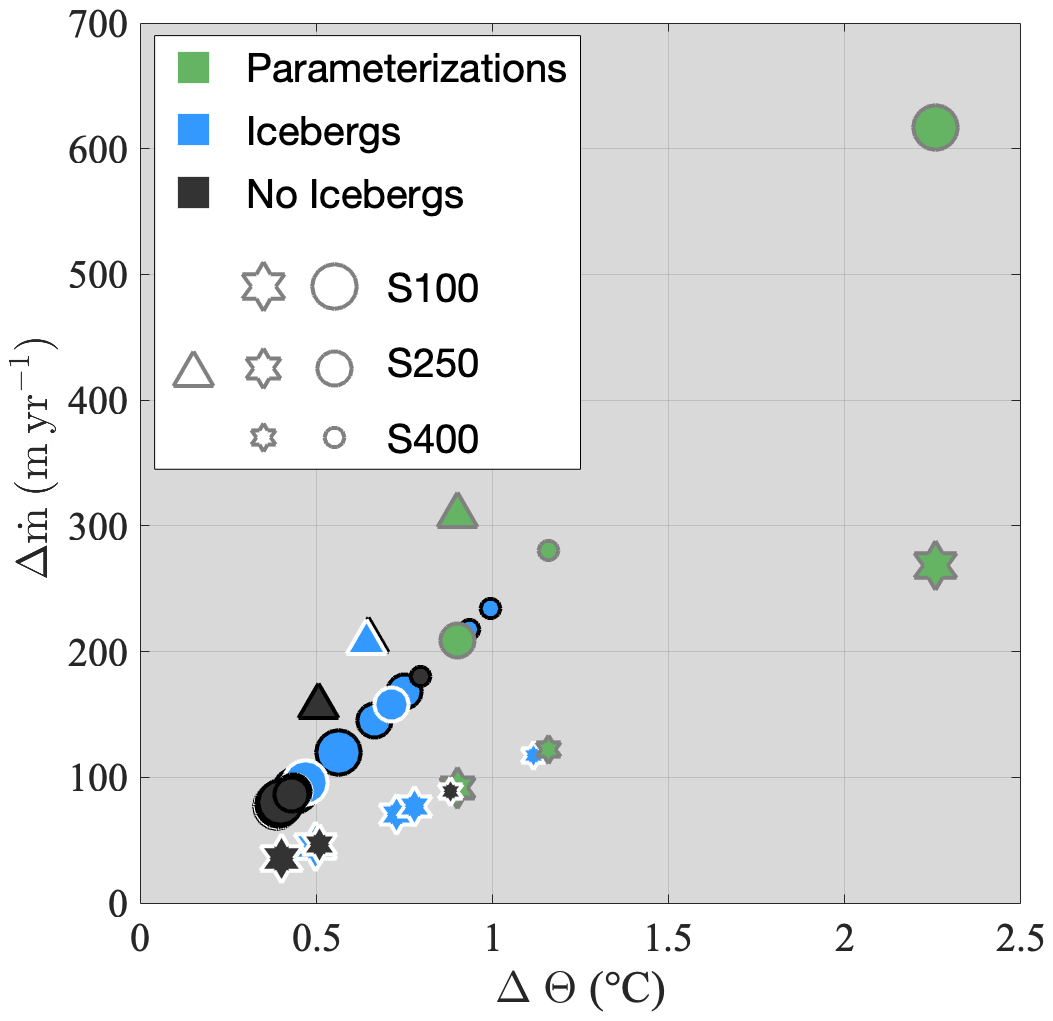
Figure 6The range of , , and for each simulation (ΔΘ), plotted with the resulting range of parameterized submarine melt rates (), as defined by Eq. (2). A ΔΘ of 0 indicates perfect agreement between , , and for a single run, while a large ΔΘ indicates these thermal forcing metrics vary substantially. Iceberg runs are light blue, and non-iceberg runs are gray. White-edged markers depict runs with line plumes, stars represent winter (Qsg = 10 m3 s−1) simulations, and triangles indicate low-resolution (Qsg = 1000 m3 s−1) runs. Marker size varies by the sill depth. Green markers depict the range of all seven thermal forcing parameterizations for each sill depth and subglacial discharge group, again plotted against the resultant range of parameterized submarine melt rates. For green markers, a ΔΘ of 0 indicates perfect agreement between all seven thermal forcing parameterizations, while a large ΔΘ indicates substantial variation between parameterizations.
Our modeling indicates that the magnitude of thermal forcing used in ice sheet models, and thus parameterized submarine melt rates, is highly sensitive to the depth range where thermal forcing is defined. In a given simulation, , , and differed by 0.4–1.1 °C (Table 1, Fig. 6), which can translate to a difference of > 200 m yr−1 in submarine melt rates parameterized by Eq. (2) (Fig. 6). An even greater thermal forcing range existed between the seven parameterizations tested in this paper (Table 2). Within a given run, thermal forcing parameterizations ranged from 0.90–2.26 °C (Fig. 6). Depending on the thermal forcing method used, submarine melt rates parameterized by Eq. (2) could therefore differ by 91–617 m yr−1 for a single fjord (Fig. 6). Melt rate parameterization uncertainty of this magnitude (≤ 1.7 m d−1) could significantly impact long-term projections of submarine melt for some Greenland glaciers (compare to projected melt rates in Fig. 10 of Slater et al., 2020). The range of parameterizations was greatest in S100 summer runs, largely due to the pronounced bathymetric effects that ISMIP6retreat and AMretreat do not account for. Also notable is the difference between thermal forcing parameterizations in our Kangiata Sullua-style low-resolution runs (Fig. 6), which due to the high subglacial discharge of Sermeq Kujalleq would contribute an uncertainty in parameterized submarine melt rates of > 300 m yr−1. Sermeq Kujalleq single-handedly accounts for 10 % of GrIS mass loss (Smith et al., 2020) and dominates uncertainty in mass balance projections of central West Greenland (Goelzer et al., 2020). Therefore, this wide range between thermal forcing parameterizations could signify substantial uncertainty in the projected terminus position of Sermeq Kujalleq and thus mass loss projections for the GrIS as a whole.
4.4 Remaining uncertainty associated with sill-driven mixing
While AMberg effectively parameterizes the two largest sources of uncertainty in predicting near-glacier thermal forcing – bathymetric obstruction and iceberg meltwater – it does not account for the modification of deep water through sill-driven reflux, which was found to be significant in this study and in previous work (Hager et al., 2022; Davison et al., 2022; Kajanto et al., 2023; Bao and Moffat, 2024). As discussed in Sect. 3.1, the influence of reflux is difficult to discern through EOF analysis, although multiple lines of evidence highlight its importance in shallow-silled fjords. First, heat reflux has the potential to exceed even the greatest iceberg heat fluxes and is responsible for the cooling of deep water (88 % of the water column in S100 runs) by up to ∼ 0.6 °C (Fig. 4). Second, the RMSE of each parameterization is greatest in S100 runs, in which more than 37 % of outflow water is refluxed. This is true despite correcting for the bathymetric obstruction of external water in most parameterizations. Thus, there must be an additional source of error related to the sill depth, which can only be explained through the cooling of deep water through the reflux of iceberg meltwater and subglacial discharge.
Deep-water cooling from sill-driven mixing is not expected to be important in fjords with sills deeper than iceberg keels or the summer terminal plume depth; however, reflux is likely influential in a number of critical glacial fjord systems. Only 10 individual glaciers are responsible for the majority of GrIS mass loss (Fahrner et al., 2021), 3 of which, Kakiffaat Sermiat, Sverdrup Gletsjer, and Sermeq Kujalleq, terminate in fjords with sills ≲ 250 m deep (as compared to grounding line depths of 400–800 m) (Morlighem et al., 2017). It is in these fjords that we expect heat reflux to significantly influence near-glacier temperatures. Indeed, recent modeling of Kangiata Sullua indicates the sill-driven reflux of iceberg meltwater cools near-glacier water by 0.2 °C (Kajanto et al., 2023), a result shared by our Kangiata Sullua-style low-resolution runs.
Although the updated parameterizations presented in this paper greatly reduce thermal forcing error compared to existing ISMIP6 methods, incorporation of sill-driven mixing could further reduce error in shallow-silled fjords, such as the Kangiata Sullua–Sermeq Kujalleq system. We anticipate such improvements would require the use of box models that contain representations of iceberg melting, subglacial discharge, and reflux. The strong linear dependence of on (Fig. 4b) indicates reflux fractions can be accurately estimated from the vertical distribution of freshwater fluxes in the water column, without any knowledge of tidal forcing. Thus, Eq. (12) could be used within a box model to predict reflux, assuming the model can approximate freshwater fluxes throughout the water column.
In summary, we have tested the accuracy of common ocean thermal forcing parameterizations across a wide range of local forcing scenarios and fjord geometries and identified fjord bathymetry and iceberg-melt-driven cooling as the two greatest sources of error when translating regional water properties to tidewater glacier termini. Even a simple adjustment for fjord bathymetry, as done in the ISMIP6 submarine melt implementation, can predict grounding line thermal forcing within an average error of 0.2 °C; however, without accounting for bathymetry, parameterizations overpredict thermal forcing by at least 2 °C in our idealized shallow-silled fjords.
Neither ISMIP6 parameterization could reliably reproduce an entire profile of near-glacier thermal forcing in our simulations due to iceberg-driven cooling of the upper water column. To address this concern, we made a simple correction to the ISMIP6 submarine melt implementation that can predict the near-glacier thermal forcing profiles of our iceberg-laden runs, as well as observed thermal forcing within Kangiata Sullua, to a skill score of > 0.90. While promising, this approach sacrifices accuracy in fjords with few icebergs and thus would be best utilized in conjunction with an iceberg prevalence prediction method, which could apply the iceberg parameterization only to fjords where iceberg melt is significant.
Our modeling also highlights the sensitivity of thermal forcing – and therefore the parameterized submarine melt rate – to the depth range that is chosen. The uncertainty this contributes to thermal forcing in ice sheet models could be substantial, and determining where best to define thermal forcing at a calving face should be a topic of high importance. For example, if a depth range that incorporates surface layers is chosen, a calving front area-mean thermal forcing, then iceberg-driven cooling becomes important and can reduce the prescribed thermal forcing by 1 °C in many Greenland fjords. Regardless, the AMfit parameterization presented here can predict entire near-glacier thermal forcing profiles with an average skill score of 0.82 across all bathymetries and iceberg concentrations tested in our simulations. As such, AMfit could be used to accurately parameterize , , , or an entire Θ(z) profile, depending on the requirements and capabilities of the ice sheet model. This result highlights the need for an iceberg prevalence prediction method to be developed and implemented in the next generation of ice sheet models.
Additional improvements to the parameterizations presented here could take the form of a box model that can effectively represent sill-driven reflux. While such an approach is outside the scope of this paper, we have identified a strong linear relationship between reflux and the ratio of freshwater released below the sill depth (Eq. 12), which we suggest could be used to efficiently estimate reflux in box models of Greenland fjords. We emphasize that such models also need to accurately parameterize iceberg melting and subglacial discharge plumes, as well as incorporate local fjord bathymetry. Still, the revised thermal forcing parameterizations presented in this paper are an improvement to existing methods, while their simplicity makes them relatively straightforward to implement. Limited observational evidence throughout Greenland supports the efficacy of these thermal forcing parameterizations, yet robust validation is still needed in realistic settings.
Efflux–reflux theory quantifies the net effect of mixing without the need to resolve individual mixing processes (Cokelet and Stewart, 1985). Effectively, efflux–reflux transports can be thought of as the vertical equivalent of the horizontal TEF budget (MacCready et al., 2021). In TEF terms, mass and volume conservation require
where superscripts o and g denote the TEF transports on the oceanward and glacierward sides of the mixing zone, respectively, and subscripts indicate whether the transport is inflowing (glacierward) or outflowing (oceanward). Superscripts on α signify the percent of the inflowing or outflowing layer that is refluxed () or effluxed () at the sill (Fig. A1). The solutions to Eq. (A1) are
Mass and volume conservation also require
and
TEF budgets are not exact, and even at a steady state some drift still occurs within the mixing zone; therefore, we make minor adjustments to the TEF transports, ensuring Eqs. (A1), (A3), and (A4) are satisfied before solving Eq. (A2) (e.g., MacCready et al., 2021; Hager et al., 2022), but the resultant error in was ≤ 0.04 % of the reported value.
Hydrographic properties were observed via helicopter-based XCTD casts within Kangiata Sullua (four profiles in August 2014 and five in August 2019) and by shipboard CTD casts in Disko Bay (four profiles in August 2014 and five in August 2019). In both years, an additional XCTD profile was obtained in Disko Bay for comparison with CTD casts. Shipboard CTD casts were conducted using an RBR XR-620 in 2014 and an RBRconcerto in 2019. All casts were averaged into 1 m bins and smoothed using a running mean filter with a 10 m window (comparable to our model vertical resolution) before undertaking the analysis described in Sect. 4.2. Further details about the 2014 field campaign are described in Beaird et al. (2017).
Abbreviated model output and statistics, as well as input and restart files for each simulation, are available at https://doi.org/10.5281/zenodo.7826386 (Hager et al., 2023). Full model output and processing code are available upon request. CTD data from Kangiata Sullua are also available at https://doi.org/10.5281/zenodo.7826386 (Hager et al., 2023).
Supplementary Movie S1 can be found at https://doi.org/10.5281/zenodo.10035545 (Hager, 2023). Movie S1 depicts six representative MITgcm simulations at steady state. The left column depicts simulations run without icebergs, while the right column depicts simulations run with icebergs. Sill depths are 100, 250, and 400 m in top, middle, and bottom panels, respectively. Icebergs have a maximum depth of 300 m and cover 75 % of the surface area within 10 km of the glacier face, linearly decreasing to 5 % at the entrance sill. All simulations were run with subglacial discharge of 300 m3 s−1 emanating from the center of the glacier face and a tidal velocity of 0.5 cm s−1 at the open boundary.
AOH designed and conducted the model experiments, performed the analysis, and wrote the paper. DaAS secured funding and provided guidance throughout the research process. DoAS contributed his expertise in ISMIP6 ocean thermal forcing parameterizations that advanced the direction of research. All authors contributed to editing the manuscript.
The contact author has declared that none of the authors has any competing interests.
Publisher's note: Copernicus Publications remains neutral with regard to jurisdictional claims made in the text, published maps, institutional affiliations, or any other geographical representation in this paper. While Copernicus Publications makes every effort to include appropriate place names, the final responsibility lies with the authors.
We thank the editor, Nanna Bjørnholdt Karlsson, as well as Michele Petrini and one anonymous referee for their careful review and suggestions for improving the manuscript.
This project was funded by a National Science Foundation (NSF) grant (no. 2020447) from the Office of International Science and Engineering, as well as an NSF grant (no. 2023269) from the Arctic Natural Sciences program within the Office of Polar Programs. Donald Slater received support from a Natural Environment Research Council (NERC) Independent Research Fellowship (no. NE/T011920/1).
This paper was edited by Nanna Bjørnholt Karlsson and reviewed by Michele Petrini and one anonymous referee.
Aschwanden, A., Fahnestock, M. A., Truffer, M., Brinkerhoff, D. J., Hock, R., Khroulev, C., Mottram, R., and Khan, S. A.: Contribution of the Greenland Ice Sheet to sea level over the next millennium, Science Advances, 5, eaav9396, https://doi.org/10.1126/sciadv.aav9396, 2019. a
Bao, W. and Moffat, C.: Impact of shallow sills on circulation regimes and submarine melting in glacial fjords, The Cryosphere, 18, 187–203, https://doi.org/10.5194/tc-18-187-2024, 2024. a, b, c, d, e, f
Bartholomaus, T. C., Stearns, L. A., Sutherland, D. A., Shroyer, E. L., Nash, J. D., Walker, R. T., Catania, G., Felikson, D., Carroll, D., Fried, M. J., Noël, B. P. Y., and van den Broeke, M. R.: Contrasts in the response of adjacent fjords and glaciers to ice-sheet surface melt in West Greenland, Ann. Glaciol., 57, 25–38, https://doi.org/10.1017/aog.2016.19, 2016. a, b, c, d
Beaird, N., Straneo, F., and Jenkins, W.: Characteristics of meltwater export from Jakobshavn Isbræ and Ilulissat Icefjord, Ann. Glaciol., 58, 107–117, https://doi.org/10.1017/aog.2017.19, 2017. a, b
Black, T. E. and Joughin, I.: Multi-decadal retreat of marine-terminating outlet glaciers in northwest and central-west Greenland, The Cryosphere, 16, 807–824, https://doi.org/10.5194/tc-16-807-2022, 2022. a
Burchard, H., Bolding, K., Feistel, R., Gräwe, U., Klingbeil, K., MacCready, P., Mohrholz, V., Umlauf, L., and van der Lee, E. M.: The Knudsen theorem and the Total Exchange Flow analysis framework applied to the Baltic Sea, Prog. Oceanogr., 165, 268–286, https://doi.org/10.1016/j.pocean.2018.04.004, 2018. a
Burgard, C., Jourdain, N. C., Reese, R., Jenkins, A., and Mathiot, P.: An assessment of basal melt parameterisations for Antarctic ice shelves, The Cryosphere, 16, 4931–4975, https://doi.org/10.5194/tc-16-4931-2022, 2022. a
Carroll, D., Sutherland, D. A., Shroyer, E. L., Nash, J. D., Catania, G. A., and Stearns, L. A.: Modeling turbulent subglacial meltwater plumes: Implications for fjord-scale buoyancy-driven circulation, J. Phys. Oceanogr., 45, 2169–2185, https://doi.org/10.1175/JPO-D-15-0033.1, 2015. a, b
Carroll, D., Sutherland, D. A., Hudson, B., Moon, T., Catania, G. A., Shroyer, E. L., Nash, J. D., Bartholomaus, T. C., Felikson, D., Stearns, L. A., Noël, B. P. Y., and van den Broeke, M. R.: The impact of glacier geometry on meltwater plume structure and submarine melt in Greenland fjords, Geophys. Res. Lett., 43, 9739–9748, https://doi.org/10.1002/2016GL070170, 2016. a, b
Carroll, D., Sutherland, D. A., Shroyer, E. L., Nash, J. D., Catania, G. A., and Stearns, L. A.: Subglacial discharge-driven renewal of tidewater glacier fjords, J. Geophys. Res.-Oceans, 122, 6611–6629, https://doi.org/10.1002/2017JC012962, 2017. a, b
Choi, Y., Morlighem, M., Rignot, E., and Wood, M.: Ice dynamics will remain a primary driver of Greenland ice sheet mass loss over the next century, Communications Earth & Environment, 2, 26, https://doi.org/10.1038/s43247-021-00092-z, 2021. a
Cokelet, E. D. and Stewart, R. J.: The Exchange of Water in Fjords: The Effiux/Reflux Theory of Advective Reaches Separated by Mixing Zones, J. Geophys. Res., 90, 7287–7306, https://doi.org/10.1029/JC090iC04p07287, 1985. a, b, c, d
Cook, S. J., Christoffersen, P., Todd, J., Slater, D., and Chauché, N.: Coupled modelling of subglacial hydrology and calving-front melting at Store Glacier, West Greenland, The Cryosphere, 14, 905–924, https://doi.org/10.5194/tc-14-905-2020, 2020. a
Cowton, T., Slater, D., Sole, A., Goldberg, D., and Nienow, P.: Modeling the impact of glacial runoff on fjord circulation and submarine melt rate using a new subgrid-scale parameterization for glacial plumes, J. Geophys. Res.-Oceans, 120, 796–812, https://doi.org/10.1002/2014JC010324, 2015. a
Cowton, T., Sole, A. J., Nienow, P. W., Slater, D., and Christoffersen, P.: Linear response of east Greenland's tidewater glaciers to ocean/atmosphere warming, P. Natl. Acad. Sci. USA, 115, 7907–7912, https://doi.org/10.1073/pnas.1801769115, 2018. a
Davison, B. J., Cowton, T. R., Cottier, F. R., and Sole, A. J.: Iceberg melting substantially modifies oceanic heat flux towards a major Greenlandic tidewater glacier, Nat. Commun., 11, 5983, https://doi.org/10.1038/s41467-020-19805-7, 2020. a, b, c, d
Davison, B. J., Cowton, T., Sole, A., Cottier, F., and Nienow, P.: Modelling the effect of submarine iceberg melting on glacier-adjacent water properties, The Cryosphere, 16, 1181–1196, https://doi.org/10.5194/tc-16-1181-2022, 2022. a, b
Ebbesmeyer, C. C. and Barnes, C. A.: Control of a fjord basin's dynamics by tidal mixing in embracing sill zones, Estuar. Coast. Mar. S., 11, 311–330, https://doi.org/10.1016/S0302-3524(80)80086-7, 1980. a
Echelmeyer, K. and Harrison, W. D.: Jakobshavns Isbræ, West Greenland: Seasonal variations in velocity-or lack thereof, J. Glaciol., 36, 82–88, 1990. a
Enderlin, E. M., Howat, I. M., Jeong, S., Noh, M.-J., Van Angelen, J. H., and Van Den Broeke, M. R.: An improved mass budget for the Greenland ice sheet, Geophys. Res. Lett., 41, 866–872, https://doi.org/10.1002/2013GL059010, 2014. a, b, c
Enderlin, E. M., Hamilton, G. S., Straneo, F., and Sutherland, D. A.: Iceberg meltwater fluxes dominate the freshwater budget in Greenland's iceberg-congested glacial fjords, Geophys. Res. Lett., 43, 11,287–11,294, https://doi.org/10.1002/2016GL070718, 2016. a, b, c
Fahrner, D., Lea, J. M., Brough, S., Mair, D. W., and Abermann, J.: Linear response of the Greenland ice sheet's tidewater glacier terminus positions to climate, J. Glaciol., 67, 193–203, https://doi.org/10.1017/jog.2021.13, 2021. a, b, c
Fox-Kemper, B., Hewitt, H., Xiao, C., Aðalgeirsdóttir, G., Drijffhour, S., Edwards, T., Golledge, N., Hemer, M., Kopp, R., Krinner, G., Mix, A., Notz, D., Nowicki, S., Nurhati, I., Ruiz, L., Sallée, J.-B., Slangen, A., and Yu, Y.: Ocean, Cryosphere, and Sea Level Change, in: Climate Change 2021: The Physical Basis. Contribution of Working Group I to the Sixth Assessment Report of the Intergovernmental Panel on Climate Change, edited by: Masson-Delmotte, V., Zhai, P., Pirani, A., Connors, S., Péan, C., Berger, S., Caud, N., Chen, Y., Goldfarb, L., Gomis, M., Huang, M., Leitzell, K., Lonnoy, E., Matthews, J., Maycock, T., Waterfield, T., Yelekçi, O., Yu, R., and Zhou, B., Cambridge University Press, Cambridge, United Kingdom and New York, NY, USA, https://doi.org/10.1017/9781009157896.011, pp. 1211–1362, 2021. a
Fried, M., Carroll, D., Catania, G., Sutherland, D., Stearns, L. A., Shroyer, E., and Nash, J.: Distinct frontal ablation processes drive heterogeneous submarine terminus morphology, Geophys. Res. Lett., 46, 12083–12091, https://doi.org/10.1029/2019GL083980, 2019. a
Gade, H. G.: Melting of ice in sea water: A primitive model with application to the Antarctic ice shelf and icebergs, J. Phys. Oceanogr., 9, 189–198, https://doi.org/10.1175/1520-0485(1979)009<0189:MOIISW>2.0.CO;2, 1979. a
Gladish, C. V., Holland, D. M., Rosing-Asvid, A., Behrens, J. W., and Boje, J.: Oceanic boundary conditions for Jakobshavn Glacier. Part I: Variability and renewal of Ilulissat Icefjord waters, 2001–14, J. Phys. Oceanogr., 45, 3–32, https://doi.org/10.1175/JPO-D-14-0044.1, 2015. a, b
Goelzer, H., Nowicki, S., Payne, A., Larour, E., Seroussi, H., Lipscomb, W. H., Gregory, J., Abe-Ouchi, A., Shepherd, A., Simon, E., Agosta, C., Alexander, P., Aschwanden, A., Barthel, A., Calov, R., Chambers, C., Choi, Y., Cuzzone, J., Dumas, C., Edwards, T., Felikson, D., Fettweis, X., Golledge, N. R., Greve, R., Humbert, A., Huybrechts, P., Le clec'h, S., Lee, V., Leguy, G., Little, C., Lowry, D. P., Morlighem, M., Nias, I., Quiquet, A., Rückamp, M., Schlegel, N.-J., Slater, D. A., Smith, R. S., Straneo, F., Tarasov, L., van de Wal, R., and van den Broeke, M.: The future sea-level contribution of the Greenland ice sheet: a multi-model ensemble study of ISMIP6, The Cryosphere, 14, 3071–3096, https://doi.org/10.5194/tc-14-3071-2020, 2020. a, b, c
Golaz, J.-C., Caldwell, P. M., Van Roekel, L. P., et al.: The DOE E3SM coupled model version 1: Overview and evaluation at standard resolution, J. Adv. Model. Earth Sy., 11, 2089–2129, https://doi.org/10.1029/2018MS001603, 2019. a
Goliber, S., Black, T., Catania, G., Lea, J. M., Olsen, H., Cheng, D., Bevan, S., Bjørk, A., Bunce, C., Brough, S., Carr, J. R., Cowton, T., Gardner, A., Fahrner, D., Hill, E., Joughin, I., Korsgaard, N. J., Luckman, A., Moon, T., Murray, T., Sole, A., Wood, M., and Zhang, E.: TermPicks: a century of Greenland glacier terminus data for use in scientific and machine learning applications, The Cryosphere, 16, 3215–3233, https://doi.org/10.5194/tc-16-3215-2022, 2022. a
Hager, A.: “Local Forcing Mechanisms challenge parameterizations of ocean thermal forcing for Greenland tidewater glaciers” – Movie S1, Zenodo [video], https://doi.org/10.5281/zenodo.10035545, 2023. a, b, c, d
Hager, A. O., Sutherland, D. A., Amundson, J. M., Jackson, R. H., Kienholz, C., Motyka, R. J., and Nash, J. D.: Subglacial discharge reflux and buoyancy forcing drive seasonality in a silled glacial fjord, J. Geophys. Res.-Oceans, 127, e2021JC018355, https://doi.org/10.1029/2021JC018355, 2022. a, b, c, d, e, f, g, h, i, j, k
Hager, A. O., Sutherland, D. A., and Slater, D. A.: Local forcing mechanisms challenge parameterizations of ocean thermal forcing for Greenland tidewater glaciers. The Cryosphere, Zenodo [data set], https://doi.org/10.5281/zenodo.7826386, 2023. a, b
Hasholt, B., Hansen, B. U., Humlum, O., and Mernild, S. H.: Meteorological stations at the Sermilik Station, Southeast Greenland: Physical environment and meteorological observations 2002, Geogr. Tidsskr., 104, 47–58, https://doi.org/10.1080/00167223.2004.10649518, 2004. a
Holland, D. M., Thomas, R. H., De Young, B., Ribergaard, M. H., and Lyberth, B.: Acceleration of Jakobshavn Isbræ triggered by warm subsurface ocean waters, Nat. Geosci., 1, 659–664, https://doi.org/10.1038/ngeo316, 2008. a, b
Howard, S. and Padman, L.: Gr1kmTM: Greeland 1 kilometer Tide Model, Arctic Data Center, https://doi.org/10.18739/A2251FM3S, 2021. a
IPCC: Climate Change 2021 – The Physical Science Basis: Working Group I Contribution to the Sixth Assessment Report of the Intergovernmental Panel on Climate Change, Cambridge University Press, Cambridge, https://doi.org/10.1017/9781009157896, 2023. a
Jackson, R. H. and Straneo, F.: Heat, salt, and freshwater budgets for a glacial fjord in Greenland, J. Phys. Oceanogr., 46, 2735–2768, https://doi.org/10.1175/JPO-D-15-0134.1, 2016. a
Jackson, R. H., Shroyer, E. L., Nash, J. D., Sutherland, D. A., Carroll, D., Fried, M. J., Catania, G. A., Bartholomaus, T. C., and Stearns, L. A.: Near-glacier surveying of a subglacial discharge plume: Implications for plume parameterizations, Geophys. Res. Lett., 44, 6886–6894, https://doi.org/10.1002/2017GL073602, 2017. a
Jackson, R. H., Nash, J. D., Kienholz, C., Sutherland, D. A., Amundson, J. M., Motyka, R. J., Winters, D., Skyllingstad, E., and Pettit, E. C.: Meltwater Intrusions Reveal Mechanisms for Rapid Submarine Melt at a Tidewater Glacier, Geophys. Res. Lett., 47, e2019GL085335, https://doi.org/10.1029/2019GL085335, 2020. a, b, c
Jakobsson, M., Mayer, L. A., Nilsson, J., Stranne, C., Calder, B., O'Regan, M., Farrell, J. W., Cronin, T. M., Brüchert, V., Chawarshi, J., Eriksson, B., Frederiksson, J., Gemery, L., Glueder, A., Holmes, F. A., Jerram, K., Kirchner, N., Mix, A., Muchowski, J., Prakash, A., Reilly, B., Thornton, B., Ulfsbo, A., Weidner, E., Åkesson, H., Handl, T., Ståhl, E., Boze, L., Reed, S., West, G., and Padman, J.: Ryder Glacier in northwest Greenland is shielded from warm Atlantic water by a bathymetric sill, Communications Earth & Environment, 1, 1–10, https://doi.org/10.1038/s43247-020-00043-0, 2020. a, b, c
Jenkins, A.: Convection-driven melting near the grounding lines of ice shelves and tidewater glaciers, J. Phys. Oceanogr., 41, 2279–2294, https://doi.org/10.1175/JPO-D-11-03.1, 2011. a, b, c
Jourdain, N. C., Asay-Davis, X., Hattermann, T., Straneo, F., Seroussi, H., Little, C. M., and Nowicki, S.: A protocol for calculating basal melt rates in the ISMIP6 Antarctic ice sheet projections, The Cryosphere, 14, 3111–3134, https://doi.org/10.5194/tc-14-3111-2020, 2020. a, b
Kajanto, K., Straneo, F., and Nisancioglu, K.: Impact of icebergs on the seasonal submarine melt of Sermeq Kujalleq, The Cryosphere, 17, 371–390, https://doi.org/10.5194/tc-17-371-2023, 2023. a, b, c, d, e, f
Knudsen, M.: Ein hydrographischer lehrsatz, Annalen der Hydrographie und Maritimen Meteorologie, 28, 316–320, 1900. a
Large, W. G., McWilliams, J. C., and Doney, S. C.: Oceanic vertical mixing: A review and a model with a nonlocal boundary layer parameterization, Rev. Geophys., 32, 363–403, https://doi.org/10.1029/94RG01872, 1994. a
Lorenz, M., Klingbeil, K., MacCready, P., and Burchard, H.: Numerical issues of the Total Exchange Flow (TEF) analysis framework for quantifying estuarine circulation, Ocean Sci., 15, 601–614, https://doi.org/10.5194/os-15-601-2019, 2019. a, b
Luckman, A., Benn, D. I., Cottier, F., Bevan, S., Nilsen, F., and Inall, M.: Calving rates at tidewater glaciers vary strongly with ocean temperature, Nat. Commun., 6, 1–7, https://doi.org/10.1038/ncomms9566, 2015. a
Ma, Y. and Bassis, J. N.: The effect of submarine melting on calving from marine terminating glaciers, J. Geophys. Res.-Earth, 124, 334–346, https://doi.org/10.1029/2018JF004820, 2019. a
MacCready, P.: Calculating estuarine exchange flow using isohaline coordinates, J. Phys. Oceanogr., 41, 1116–1124, https://doi.org/10.1175/2011JPO4517.1, 2011. a, b
MacCready, P., Geyer, W. R., and Burchard, H.: Estuarine exchange flow is related to mixing through the salinity variance budget, J. Phys. Oceanogr., 48, 1375–1384, https://doi.org/10.1175/JPO-D-17-0266.1, 2018. a
MacCready, P., McCabe, R. M., Siedlecki, S. A., Lorenz, M., Giddings, S. N., Bos, J., Albertson, S., Banas, N. S., and Garnier, S.: Estuarine Circulation, Mixing, and Residence Times in the Salish Sea, J. Geophys. Res.-Oceans, 126, e2020JC016738, https://doi.org/10.1029/2020JC016738, 2021. a, b, c, d, e
Magorrian, S. J. and Wells, A. J.: Turbulent plumes from a glacier terminus melting in a stratified ocean, J. Geophys. Res.-Oceans, 121, 4670–4696, https://doi.org/10.1002/2015JC011160, 2016. a
Mankoff, K. D., Straneo, F., Cenedese, C., Das, S. B., Richards, C. G., and Singh, H.: Structure and dynamics of a subglacial discharge plume in a G reenlandic fjord, J. Geophys. Res.-Oceans, 121, 8670–8688, https://doi.org/10.1002/2016JC011764, 2016. a, b
Marshall, J., Adcroft, A., Hill, C., Perelman, L., and Heisey, C.: A finite-volume, incompressible Navier Stokes model for studies of the ocean on parallel computers, J. Geophys. Res.-Oceans, 102, 5753–5766, https://doi.org/10.1029/96JC02775, 1997. a
McDougall, T. and Barker, P.: Getting started with TEOS-10 and the Gibbs Seawater (GSW) Oceanographic Toolbox, SCOR/IAPSO Working Group 127, http://www.teos-10.org/ (last access: 20 February 2024), 2011. a
Moffat, C., Tapia, F. J., Nittrouer, C. A., Hallet, B., Bown, F., Boldt Love, K., and Iturra, C.: Seasonal evolution of ocean heat supply and freshwater discharge from a rapidly retreating tidewater glacier: Jorge Montt, Patagonia, J. Geophys. Res.-Oceans, 123, 4200–4223, https://doi.org/10.1002/2017JC013069, 2018. a, b
Mojica, J. F., Djoumna, G., Holland, D. M., and Holland, D.: Interannual summer mixing processes in the Ilulissat Icefjord, Greenland, J. Marine Syst., 214, 103476, https://doi.org/10.1016/j.jmarsys.2020.103476, 2021. a
Moon, T., Sutherland, D. A., Carroll, D., Felikson, D., Kehrl, L., and Straneo, F.: Subsurface iceberg melt key to Greenland fjord freshwater budget, Nat. Geosci., 11, 49–54, https://doi.org/10.1038/s41561-017-0018-z, 2018. a, b, c, d, e
Morlighem, M., Bondzio, J., Seroussi, H., Rignot, E., Larour, E., Humbert, A., and Rebuffi, S.: Modeling of Store Gletscher's calving dynamics, West Greenland, in response to ocean thermal forcing, Geophys. Res. Lett., 43, 2659–2666, https://doi.org/10.1002/2016GL067695, 2016. a
Morlighem, M., Williams, C. N., Rignot, E., Arndt, J. E., Bamber, J. L., Catania, G., Chauché, N. Dowdeswell, J. A., Dorschel, B., Fenty, I., Hogan, K., Howat, I., Hubbard, A., Jakobsson, M., Jordan, T. M., Kjeldsen, K. K., Millan, R., Mayer, L., Mouginot, J., Noël B. P. Y., O'Cofaigh, C., Palmer, S., Rysgaard, S., Seroussi, H., Siegert, M. J., Slabon, P., Straneo, F., van den Broeke, M. R., Weinrebe, W., Wood, M., and Zinglersen, K. B.: BedMachine v3: Complete bed topography and ocean bathymetry mapping of Greenland from multibeam echo sounding combined with mass conservation, Geophys. Res. Lett., 44, 11–051, https://doi.org/10.1002/2017GL074954, 2017. a
Morlighem, M., Wood, M., Seroussi, H., Choi, Y., and Rignot, E.: Modeling the response of northwest Greenland to enhanced ocean thermal forcing and subglacial discharge, The Cryosphere, 13, 723–734, https://doi.org/10.5194/tc-13-723-2019, 2019. a, b, c, d
Mortensen, J., Lennert, K., Bendtsen, J., and Rysgaard, S.: Heat sources for glacial melt in a sub-Arctic fjord (Godthåbsfjord) in contact with the Greenland Ice Sheet, J. Geophys. Res.-Oceans, 116, C01013, https://doi.org/10.1029/2010JC006528, 2011. a
Mortensen, J., Bendtsen, J., Motyka, R. J., Lennert, K., Truffer, M., Fahnestock, M., and Rysgaard, S.: On the seasonal freshwater stratification in the proximity of fast-flowing tidewater outlet glaciers in a sub-Arctic sill fjord, J. Geophys. Res.-Oceans, 118, 1382–1395, https://doi.org/10.1002/jgrc.20134, 2013. a, b
Mortensen, J., Bendtsen, J., Lennert, K., and Rysgaard, S.: Seasonal variability of the circulation system in a west Greenland tidewater outlet glacier fjord, Godthåbsfjord (64 N), J. Geophys. Res.-Earth, 119, 2591–2603, 2014. a
Motyka, R. J., Truffer, M., Fahnestock, M., Mortensen, J., Rysgaard, S., and Howat, I.: Submarine melting of the 1985 Jakobshavn Isbræ floating tongue and the triggering of the current retreat, J. Geophys. Res.-Earth, 116, F01007, https://doi.org/10.1029/2009JF001632, 2011. a
Mouginot, J., Rignot, E., Bjørk, A. A., Van den Broeke, M., Millan, R., Morlighem, M., Noël, B., Scheuchl, B., and Wood, M.: Forty-six years of Greenland Ice Sheet mass balance from 1972 to 2018, P. Natl. Acad. Sci. USA, 116, 9239–9244, 2019. a
Murray, T., Scharrer, K., James, T., Dye, S., Hanna, E., Booth, A., Selmes, N., Luckman, A., Hughes, A., Cook, S., and Huybrechts, P.: Ocean regulation hypothesis for glacier dynamics in southeast Greenland and implications for ice sheet mass changes, J. Geophys. Res.-Earth, 115, F03026, https://doi.org/10.1029/2009JF001522, 2010. a, b
Nick, F. M., Vieli, A., Howat, I. M., and Joughin, I.: Large-scale changes in Greenland outlet glacier dynamics triggered at the terminus, Nat. Geosci., 2, 110–114, https://doi.org/10.1038/NGEO394, 2009. a
Nowicki, S., Goelzer, H., Seroussi, H., Payne, A. J., Lipscomb, W. H., Abe-Ouchi, A., Agosta, C., Alexander, P., Asay-Davis, X. S., Barthel, A., Bracegirdle, T. J., Cullather, R., Felikson, D., Fettweis, X., Gregory, J. M., Hattermann, T., Jourdain, N. C., Kuipers Munneke, P., Larour, E., Little, C. M., Morlighem, M., Nias, I., Shepherd, A., Simon, E., Slater, D., Smith, R. S., Straneo, F., Trusel, L. D., van den Broeke, M. R., and van de Wal, R.: Experimental protocol for sea level projections from ISMIP6 stand-alone ice sheet models, The Cryosphere, 14, 2331–2368, https://doi.org/10.5194/tc-14-2331-2020, 2020. a
Nowicki, S. M. J., Payne, A., Larour, E., Seroussi, H., Goelzer, H., Lipscomb, W., Gregory, J., Abe-Ouchi, A., and Shepherd, A.: Ice Sheet Model Intercomparison Project (ISMIP6) contribution to CMIP6, Geosci. Model Dev., 9, 4521–4545, https://doi.org/10.5194/gmd-9-4521-2016, 2016. a
O'Leary, M. and Christoffersen, P.: Calving on tidewater glaciers amplified by submarine frontal melting, The Cryosphere, 7, 119–128, https://doi.org/10.5194/tc-7-119-2013, 2013. a
Rignot, E., Xu, Y., Menemenlis, D., Mouginot, J., Scheuchl, B., Li, X., Morlighem, M., Seroussi, H., den Broeke, M. v., Fenty, I., Cai, C., and de Fleurian B.: Modeling of ocean-induced ice melt rates of five west Greenland glaciers over the past two decades, Geophys. Res. Lett., 43, 6374–6382, https://doi.org/10.1002/2016GL068784, 2016. a, b
Schild, K. M., Sutherland, D. A., Elosegui, P., and Duncan, D.: Measurements of iceberg melt rates using high-resolution GPS and iceberg surface scans, Geophys. Res. Lett., 48, e2020GL089765, https://doi.org/10.1029/2020GL089765, 2021. a
Sciascia, R., Straneo, F., Cenedese, C., and Heimbach, P.: Seasonal variability of submarine melt rate and circulation in an East Greenland fjord, J. Geophys. Res.-Oceans, 118, 2492–2506, https://doi.org/10.1002/jgrc.20142, 2013. a
Seroussi, H., Nowicki, S., Payne, A. J., Goelzer, H., Lipscomb, W. H., Abe-Ouchi, A., Agosta, C., Albrecht, T., Asay-Davis, X., Barthel, A., Calov, R., Cullather, R., Dumas, C., Galton-Fenzi, B. K., Gladstone, R., Golledge, N. R., Gregory, J. M., Greve, R., Hattermann, T., Hoffman, M. J., Humbert, A., Huybrechts, P., Jourdain, N. C., Kleiner, T., Larour, E., Leguy, G. R., Lowry, D. P., Little, C. M., Morlighem, M., Pattyn, F., Pelle, T., Price, S. F., Quiquet, A., Reese, R., Schlegel, N.-J., Shepherd, A., Simon, E., Smith, R. S., Straneo, F., Sun, S., Trusel, L. D., Van Breedam, J., van de Wal, R. S. W., Winkelmann, R., Zhao, C., Zhang, T., and Zwinger, T.: ISMIP6 Antarctica: a multi-model ensemble of the Antarctic ice sheet evolution over the 21st century, The Cryosphere, 14, 3033–3070, https://doi.org/10.5194/tc-14-3033-2020, 2020. a, b
Slater, D., Nienow, P., Cowton, T., Goldberg, D., and Sole, A.: Effect of near-terminus subglacial hydrology on tidewater glacier submarine melt rates, Geophys. Res. Lett., 42, 2861–2868, https://doi.org/10.1002/2014GL062494, 2015. a
Slater, D., Straneo, F., Das, S., Richards, C., Wagner, T., and Nienow, P.: Localized plumes drive front-wide ocean melting of a Greenlandic tidewater glacier, Geophys. Res. Lett., 45, 12–350, https://doi.org/10.1029/2018GL080763, 2018. a
Slater, D. A., Straneo, F., Felikson, D., Little, C. M., Goelzer, H., Fettweis, X., and Holte, J.: Estimating Greenland tidewater glacier retreat driven by submarine melting, The Cryosphere, 13, 2489–2509, https://doi.org/10.5194/tc-13-2489-2019, 2019. a, b, c, d
Slater, D. A., Felikson, D., Straneo, F., Goelzer, H., Little, C. M., Morlighem, M., Fettweis, X., and Nowicki, S.: Twenty-first century ocean forcing of the Greenland ice sheet for modelling of sea level contribution , The Cryosphere, 14, 985–1008, https://doi.org/10.5194/tc-14-985-2020, 2020. a, b, c, d, e, f, g, h
Smagorinsky, J.: General Circulation experiments with the primitive equations: I. The basic experiment, Mon. Weather Rev., 91, 99–164, https://doi.org/10.1175/1520-0493(1963)091<0099:GCEWTP>2.3.CO;2, 1963. a
Smith, B., Fricker, H. A., Gardner, A. S., Medley, B., Nilsson, J., Paolo, F. S., Holschuh, N., Adusumilli, S., Brunt, K., Csatho, B., Harbeck, K., Markus, T., Neumann, T., Siegfried, M. R., and Zwally, H. J.: Pervasive ice sheet mass loss reflects competing ocean and atmosphere processes, Science, 368, 1239–1242, https://doi.org/10.1126/science.aaz5845, 2020. a
Straneo, F. and Cenedese, C.: The dynamics of Greenland's glacial fjords and their role in climate, Annu. Rev. Mar. Sci., 7, 89–112, https://doi.org/10.1146/annurev-marine-010213-135133, 2015. a, b, c
Straneo, F. and Heimbach, P.: North Atlantic warming and the retreat of Greenland's outlet glaciers, Nature, 504, 36–43, https://doi.org/10.1038/nature12854, 2013. a, b
Straneo, F., Curry, R. G., Sutherland, D. A., Hamilton, G. S., Cenedese, C., Våge, K., and Stearns, L. A.: Impact of fjord dynamics and glacial runoff on the circulation near Helheim Glacier, Nat. Geosci., 4, 322–327, https://doi.org/10.1038/NGEO1109, 2011. a
Straneo, F., Sutherland, D. A., Holland, D., Gladish, C., Hamilton, G. S., Johnson, H. L., Rignot, E., Xu, Y., and Koppes, M.: Characteristics of ocean waters reaching Greenland's glaciers, Ann. Glaciol., 53, 202–210, https://doi.org/10.3189/2012AoG60A059, 2012. a, b, c
Sulak, D. J., Sutherland, D. A., Enderlin, E. M., Stearns, L. A., and Hamilton, G. S.: Iceberg properties and distributions in three Greenlandic fjords using satellite imagery, Ann. Glaciol., 58, 92–106, https://doi.org/10.1017/aog.2017.5, 2017. a, b, c
Sutherland, D., Jackson, R. H., Kienholz, C., Amundson, J. M., Dryer, W., Duncan, D., Eidam, E., Motyka, R., and Nash, J.: Direct observations of submarine melt and subsurface geometry at a tidewater glacier, Science, 365, 369–374, https://doi.org/10.1126/science.aax3528, 2019. a
The IMBIE Team: Mass balance of the Greenland Ice Sheet from 1992 to 2018, Nature, 579, 233–239, https://doi.org/10.1038/s41586-019-1855-2, 2019. a
van den Broeke, M. R., Enderlin, E. M., Howat, I. M., Kuipers Munneke, P., Noël, B. P. Y., van de Berg, W. J., van Meijgaard, E., and Wouters, B.: On the recent contribution of the Greenland ice sheet to sea level change, The Cryosphere, 10, 1933–1946, https://doi.org/10.5194/tc-10-1933-2016, 2016. a
Watanabe, M., Suzuki, T., O'ishi, R., Komuro, Y., Watanabe, S., Emori, S., Takemura, T., Chikira, M., Ogura, T., Sekiguchi, M., Takata, K., Yamazaki, D., Yokohata, T., Nozawa, T., Hasumi, H., Tatebe, H., and Kimoto, M.: Improved climate simulation by MIROC5: mean states, variability, and climate sensitivity, J. Climate, 23, 6312–6335, https://doi.org/10.1175/2010JCLI3679.1, 2010. a
Willmott, C. J.: On the validation of models, Phys. Geogr., 2, 184–194, https://doi.org/10.1080/02723646.1981.10642213, 1981. a
Wood, M., Rignot, E., Fenty, I., Menemenlis, D., Millan, R., Morlighem, M., Mouginot, J., and Seroussi, H.: Ocean-induced melt triggers glacier retreat in Northwest Greenland, Geophys. Res. Lett., 45, 8334–8342, https://doi.org/10.1029/2018GL078024, 2018. a
Xu, Y., Rignot, E., Menemenlis, D., and Koppes, M.: Numerical experiments on subaqueous melting of Greenland tidewater glaciers in response to ocean warming and enhanced subglacial discharge, Ann. Glaciol., 53, 229–234, https://doi.org/10.3189/2012AoG60A139, 2012. a
- Abstract
- Introduction
- Methods
- Results
- Discussion
- Conclusions
- Appendix A: Total exchange flow (TEF) and efflux–reflux theory
- Appendix B: Collection and processing of hydrographic data
- Appendix C: Parameterization flowchart
- Data availability
- Video supplement
- Author contributions
- Competing interests
- Disclaimer
- Acknowledgements
- Financial support
- Review statement
- References