the Creative Commons Attribution 4.0 License.
the Creative Commons Attribution 4.0 License.
 | 19 Feb 2024
A low-cost and open-source approach for supraglacial debris thickness mapping using UAV-based infrared thermography
Jérôme Messmer
Alexander Raphael Groos
Debris-covered glaciers exist in many mountain ranges and play an important role in the regional water cycle. However, modelling the surface mass balance, runoff contribution and future evolution of debris-covered glaciers is fraught with uncertainty as accurate observations on small-scale variations in debris thickness and sub-debris ice melt rates are only available for a few locations worldwide. Here we describe a customised low-cost unoccupied aerial vehicle (UAV) for high-resolution thermal imaging of mountain glaciers and present a complete open-source pipeline that facilitates the generation of accurate surface temperature and debris thickness maps from radiometric images. First, a radiometric orthophoto is computed from individual radiometric UAV images using structure-from-motion and multi-view-stereo techniques. User-specific calibration and correction procedures can then be applied to the radiometric orthophoto to account for atmospheric and environmental influences that affect the radiometric measurement. The thermal orthophoto reveals distinct spatial variations in surface temperature across the surveyed debris-covered area. Finally, a high-resolution debris thickness map is derived from the corrected thermal orthophoto using an empirical or inverse surface energy balance model that relates surface temperature to debris thickness and is calibrated against in situ measurements. Our results from a small-scale experiment on the Kanderfirn (also known as Kander Neve) in the Swiss Alps show that the surface temperature and thickness of a relatively thin debris layer (ca. 0–15 cm) can be mapped with high accuracy using an empirical or physical model. On snow and ice surfaces, the mean deviation of the mapped surface temperature from the melting point (∼ 0 ∘C) was 0.6 ± 2.0 ∘C. The root-mean-square error of the modelled debris thickness was 1.3 cm. Through the detailed mapping, typical small-scale debris features and debris thickness patterns become visible, which are not spatially resolved by the thermal infrared sensors of current-generation satellites. The presented approach paves the way for comprehensive high-resolution supraglacial debris thickness mapping and opens up new opportunities for more accurate monitoring and modelling of debris-covered glaciers.
- Article
(14990 KB) - Full-text XML
- BibTeX
- EndNote


Supraglacial debris is present in the ablation zone of many mountain glaciers worldwide (Scherler et al., 2018; Herreid and Pellicciotti, 2020) and can influence their mass balance, geometry and dynamics through the modification of sub-debris ice melt rates (e.g. Rowan et al., 2015; Ferguson and Vieli, 2020; Mayer and Licciulli, 2021; Rounce et al., 2021; Delaney and Anderson, 2022). Important sources of debris supply are steep headwalls, valley slopes and lateral moraines, and subglacial till (e.g. Anderson et al., 2018; van Woerkom et al., 2019). Debris can be mobilised and transported onto glaciers by gravitational mass movements such as avalanches, landslides and rockfalls. Debris deposited on the glacier surface, as well as debris melted out of the ice, accumulates in the ablation zone and often forms a continuous debris layer (e.g. Anderson et al., 2018; Wirbel et al., 2018; Ferguson and Vieli, 2020; Mayer and Licciulli, 2021). The thickness of supraglacial debris can range from less than 1 cm to more than 2 m and usually shows high spatial variability across the ablation zone. The estimated global mean supraglacial debris thickness is in the order of 30–40 cm (Rounce et al., 2021). However, debris thinner than 10 cm predominates, usually accounting for more than 50 % of the total debris-covered glacier area (Rounce et al., 2021; McCarthy et al., 2022). While thin debris (less than a few centimetres) increases melting due to its lower albedo compared to a clean-ice surface, thick debris insulates the underlying ice and reduces melting (Østrem, 1959; Nicholson and Benn, 2006; Evatt et al., 2015). Due to the reduced ice melt rate, mountain glaciers with an extensive and relatively thick debris cover are typically larger and a have a flatter and lower-situated tongue than clean-ice glaciers in a similar topographic and climatic setting (Scherler et al., 2011).
Several satellite remote sensing studies have found similar thinning rates at comparable elevations for debris-covered and clean-ice glaciers, despite their geomorphological differences (e.g. Kääb et al., 2012; Gardelle et al., 2013). Enhanced melting due to the presence of ice cliffs and supraglacial ponds in the debris-covered area and relatively low emergence velocities of debris-covered glacier tongues are discussed as possible explanations for this peculiarity (e.g. Sakai et al., 1998; Steiner et al., 2015; Brun et al., 2018; Miles et al., 2018; Anderson et al., 2021; Buri et al., 2021). However, testing these hypotheses and determining the high spatial variability of ice melt rates across debris-covered areas remains a challenge, partly due to the lack of high-resolution supraglacial debris thickness maps. For quantifying the impact of debris on the glacier mass balance and for projecting the future evolution of debris-covered glaciers and their response to ongoing climate change, accurate information on the spatial debris thickness distribution is urgently needed (Kraaijenbrink et al., 2017; Rounce et al., 2020, 2021).
Over the last 2 decades, various methods have been developed to determine the thickness of supraglacial debris. These include in situ point measurements (e.g. Mihalcea et al., 2006), terrestrial tachymetric and photogrammetric measurements of debris over ice cliffs (Nicholson and Benn, 2013; Nicholson and Mertes, 2017), and ground-penetrating radar measurements along predefined transects (McCarthy et al., 2017). For glacier-wide mapping, debris thickness can be derived from remotely sensed surface temperatures or surface elevation change rates using physical or empirical functions that relate surface temperature or sub-debris ice melt to debris thickness (e.g. Mihalcea et al., 2008a, b; Foster et al., 2012; Juen et al., 2014; Rounce and McKinney, 2014; Groos et al., 2017; Rounce et al., 2018, 2021). However, satellite remote sensing has the drawback that the acquisition time, viewing angle and atmospheric conditions cannot be controlled by the end user and might not be in favour of debris thickness mapping (e.g. Herreid, 2021). Debris thickness maps based on satellite remote sensing data usually capture general debris thickness patterns in the ablation zone but cannot resolve the small-scale debris thickness variability and the presence of melt hotspots such as supraglacial ice cliffs and ponds due to their relatively coarse spatial resolution. Since the relationship between debris thickness and sub-debris ice melt is non-linear (Østrem, 1959) and melt hotspots are not resolved, the mean debris thickness per pixel derived from relatively coarse satellite data seems not well suited to simulate sub-debris ice melt rates. To better estimate the ablation and runoff contribution of individual debris-covered glaciers, high-resolution debris thickness mapping techniques are required.
Recent advances in terrestrial and unoccupied aerial vehicle (UAV) infrared thermography offer new possibilities for mapping glacier surface temperature and supraglacial debris thickness at centimetre resolution. Ground-based thermal infrared (TIR) images have been used in previous studies to investigate thermal processes at the glacier surface (Aubry-Wake et al., 2015, 2018) and to estimate supraglacial debris thickness (Herreid, 2021; Tarca and Guglielmin, 2022; Aubry-Wake et al., 2023). However, with this approach it is difficult to survey larger areas and impractical to measure objects that are not in line of sight. UAVs equipped with lightweight TIR cameras have proven to be a suitable alternative for mapping surface temperatures on debris-covered glaciers in mountainous terrain (Kraaijenbrink et al., 2018). Two recent studies have successfully demonstrated that debris thickness can be simulated from radiometric thermal UAV imagery if the images are carefully calibrated and corrected (Bisset et al., 2022; Gök et al., 2023). However, in the study by Bisset et al. (2022) the number of debris thickness measurements for validation was small (n=3), and in the study by Gök et al. (2023) the methodological uncertainties (a root-mean-square error, RMSE, of 6–8 cm for a mean debris thickness of 9 cm) were relatively large, highlighting the need of further exploring and developing this mapping approach.
Here we present a customised UAV for high-resolution thermal imaging on glaciers and a complete open-source pipeline that enables the generation of surface temperature and debris thickness maps from radiometric imagery. Compared to previous studies that mainly rely on proprietary software (e.g. Kraaijenbrink et al., 2018; Bisset et al., 2022; Gök et al., 2023), our open-source approach supports the generation of accurate radiometric orthophotos that can be further processed and corrected according to the users' needs. We use thermal imagery and in situ measurements of debris thickness and debris temperature from the Kanderfirn (also known as Kander Neve) in the Swiss Alps (Fig. 1) to illustrate and discuss the limitations and potential of the methodology.
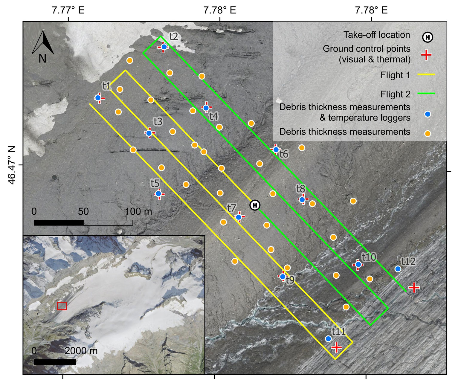
Figure 1Overview map of the thermographic UAV surveys and in situ measurements on the Kanderfirn on 28 September 2021. The location of the UAV takeoff site, ground control points, debris temperature loggers and debris thickness measurements is indicated by the respective symbols. Data source of the lower-left map inset: SWISSIMAGE from 2018 (Swiss Federal Office of Topography, 2021).
The Kanderfirn (46.47∘ N, 7.78∘ E), a southwest-facing valley glacier in the Bernese Alps, was chosen as a test site for the UAV-based thermal imaging and debris thickness mapping as it comprises both a debris-covered and debris-free area. The latter is helpful for assessing the accuracy of the thermal images (see Sect. 3.6.5). Furthermore, experience with the use of UAVs on this glacier already exists from previous campaigns (Groos et al., 2019, 2022a). The tongue of the Kanderfirn is situated at ca. 2300 m a.s.l. The highest point is the Petersgrat with an elevation of ca. 3200 m a.s.l. The area of the Kanderfirn was 16.0 km2 in 1850. It decreased to 13.8 km2 in 1973 (Maisch et al., 2000; Paul, 2003) and to 12.2 km2 in 2010. Today it is less than 12.0 km2 (Fischer et al., 2014; Groos et al., 2019). An area of around 1 km2 in the northwestern part of the Kanderfirn is covered by debris (Swiss Federal Office of Topography, 2021). The predominant part of the debris cover on the Kanderfirn originates from the south face of the Blüemlisalp, which mainly consists of sedimentary rocks. In the southwest, granites and gneisses can be found. The lithology at the base is a mix of sedimentary and igneous rocks (Hügi, 1956; Swiss Federal Office of Topography et al., 2005). Since the entire debris-covered area is too large to be mapped with the customised quadcopter (see Sect. 3.1), only part of it was surveyed in this study (see Fig. 1). The elevation of the surveyed debris-covered area ranges from 2425 to 2480 m a.s.l. and is cut by two parallel meltwater streams running from northeast to southwest. The inclined areas (mean slope = 15∘; standard deviation = 10∘) face predominantly towards northwest and southeast.
3.1 Customised low-cost UAV
A small commercial rotary-wing UAV, a DJI Mavic Pro, which costs less than EUR 1000 and is equipped with a lightweight TIR camera (see Fig. 2), was chosen for the thermal imaging as the entire system can be easily transported to remote locations and ensures the safe takeoff and landing of expensive and fragile sensors. The quadcopter weighs 750 g including its 43.6 Wh battery. According to the manufacturer, the maximum flight time in normal use (without additional payload) is 27 min. A global navigation satellite system (GNSS) and a forward and downward vision system is used for orientation. The quadcopter has a built-in stabilised and movable camera with a focal length of 4.7 mm, equalling a 78.8∘ field of view. The maximum resolution for still images is 3000×4000 pixels. The UAV and its camera are controlled using a handheld remote controller and smartphone (DJI, 2016).
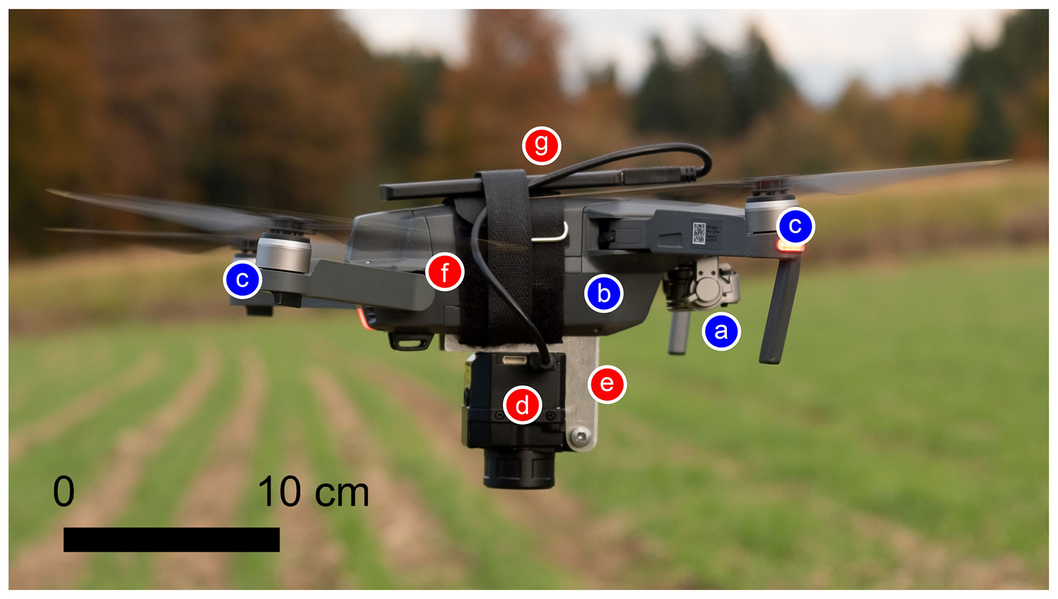
Figure 2The complete UAV setup in action during a test flight. Parts that belong to the Mavic Pro itself are marked in blue and additional parts in red: (a) UAV camera, (b) UAV body, (c) collapsible UAV arms including motors and propellers, (d) TIR camera (FLIR Vue Pro R 640), (e) customised mounting to attach the camera to the UAV body, (f) Velcro straps for the attachment of the camera mounting and external battery, and (g) battery and cable to power the camera.
The TIR camera used in this study was a FLIR Vue Pro R 640 (30 Hz) as it has been specifically designed for UAV-based applications and provides thermal imagery of similar accuracy to other, more expensive lightweight TIR cameras (Sagan et al., 2019). The Vue Pro R 640 measures cm, weighs 140 g and has a focal length of 13 mm. An uncooled vanadium oxide microbolometer is used for radiometric measurements of thermal infrared radiation in the 7.5–13.5 µm spectrum. Both still and moving images can be captured with a viewing angle of 45∘. The resolution of the thermal images is 640×512 pixels (Teledyne FLIR, 2019b). The exposure time of the camera is not specified but is estimated to be around s (Teledyne FLIR, 2019a; USGS UAS, 2019). The claimed measurement accuracy is ± 5 ∘C or 5 % of the reading. An external battery must be connected to the camera for power supply.
The TIR camera was attached to the UAV using a customised mounting system consisting of two angled aluminium plates (Fig. 2). The plates are inserted into grooves on the underside of the UAV and additionally attached to the body with two adjustable Velcro straps. This design allows for a flexible alignment and quick attachment and removal of the camera. The camera is powered with an external 11.4 Wh battery. The UAV plus camera and mounting weighs about 1 kg. It must be noted that the DJI Mavic Pro is not designed to carry loads. Additional payloads reduce the maximum flight duration and increase the risk of motor overheating and damage.
3.2 UAV-based visual and thermal infrared surveys
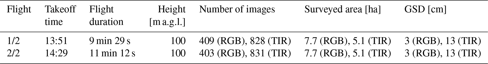
The UAV-based thermal imaging on the Kanderfirn was carried out on 28 September 2021 in the early afternoon during slightly overcast conditions (Table 1). As a compromise between ascent time, ground sampling distance (GSD) and image detail, we chose a flight height of 100 m above ground level (a.g.l.). At this height, the estimated GSD of the thermal images is 13 cm, and the image footprint is 83×67 m. The flight speed was set to 8.5 km h−1. At this speed, assuming an exposure time of 1/100 s, motion blur is 2.4 cm (18 % of the GSD). For the photogrammetric processing and orthophoto generation (see Sect. 3.5), a lateral image overlap of at least 60 % is common in UAV photogrammetry (e.g. Kraaijenbrink et al., 2018). To account for that, the distance between parallel flight tracks was set to 21 m, resulting in a lateral image overlap of 75 % for the TIR imagery and even more for the RGB imagery. A maximum flight time of 13 min could be achieved with the customised UAV. This translated into individual flight tracks of about 900–1000 m.
Table 1Key figures of the UAV surveys on 28 September 2021. GSD means ground sampling distance.
The third-party mobile application Litchi was used to fly the UAV in autonomous mode (VC Technology, 2020). A cardboard box with a cut-out hole matching the TIR camera on the underside of the UAV served as a base for manual takeoff. As landing on the box was difficult, the UAV was grabbed in hover mode from a low height after completion of the survey. The open-source geographic information system QGIS (QGIS Development Team, 2020) and the Litchi mission hub (VC Technology, 2021) served for flight planning. A UAV-based high-resolution surface model of the Kanderfirn from 2021 (Groos et al., 2022a) was uploaded to the mission hub to ensure a somewhat constant flight height above the uneven terrain. We performed two consecutive flights to survey part of the debris-covered and debris-free glacier area (see Fig. 1). Both visual and thermal images were taken with an interval of 1 s. The thermal images were stored as radiometric JPGs on the camera's SD card as only this file type contains radiometric data and allows for the accurate calculation of surface temperatures. Visual images were stored in JPG format on the UAV's SD card.
Twelve visual and 12 thermal ground control points (GCPs) were distributed across the survey area (Figs. 1 and 3) for accurate photogrammetric processing of the aerial images and for accurate georeferencing of the orthophotos. We used red Teflon sheets (A2 paper size) as visual GCPs and cardboard sheets (A3 paper size) wrapped in aluminium foil as thermal GCPs. Aluminium foil is a suitable material for thermal GCPs because it has a much lower emissivity than ice, snow, or debris and therefore appears cooler on thermal images (e.g. Kraaijenbrink et al., 2018). The position of the centre of each GCP was measured using a differential GNSS device (Trimble Geo 7x).
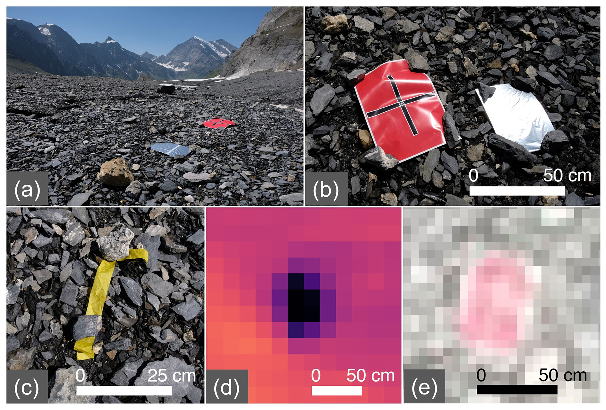
Figure 3(a) Overview of the surveyed debris cover (view towards the terminus), (b) close-up view of a visual and a thermal GCP on the debris surface, (c) yellow ribbon used to mark the position of the temperature loggers, (d) a thermal GCP as seen in a thermal UAV image and (e) a visual GCP as seen in a visual UAV image.
3.3 In situ measurements
3.3.1 Debris thickness
As a basis for the calibration and validation of the applied debris thickness models (see Sect. 3.7), we measured supraglacial debris thickness randomly at 43 points across the survey area while being in the field (Fig. 1). Only areas that were completely covered by debris or fine material were sampled. Since the debris thickness was only a few centimetres at most locations, holes could be manually dug in the debris layer until the ice surface was reached. We measured the depths of the debris with a folding ruler and determined the exact position of each in situ measurement with the differential GNSS device.
3.3.2 Debris temperature
At 12 locations, corresponding to the locations of the debris thickness measurements d1–d12, we installed button-sized, splash-proof tempmate.-B2 temperature loggers in the debris (see Fig. 1) for a rough comparison with the UAV-based thermal imaging (see Sect. 3.6.5). Since the tiny temperature loggers recorded the debris temperature at shallow depths and the TIR camera mounted on the UAV measured the skin temperature of the debris layer, the in situ measurements and mapped surface temperatures cannot be expected to match exactly. However, a cross-comparison makes it possible to detect a potential warm or cold bias in the camera and assess the plausibility of the mapped debris surface temperatures. The loggers' measurement accuracy is ±0.5 ∘C in the range from −10 to 65 ∘C (Tempmate, 2022). Groos et al. (2022b) have shown in a previous study that the tiny temperature loggers are suitable for ground temperature measurements in high-mountain environments. We placed each logger under a 0.5–1.0 cm thick shale stone to protect it from direct radiation and measured its position with the differential GNSS device. Because the temperature loggers are small and low in contrast to the debris, we marked their location with a yellow ribbon (Fig. 3). The loggers were set to record temperature at an interval of 10 min and were running for about an hour before the survey so that they could become isothermal with their environment. The mean of all temperature readings between capture time of the first and last thermal image used for orthophoto creation was calculated for each temperature logger. Prior to the field campaign, we conducted an indoor comparison measurement at around 20 ∘C. In the comparison measurement, no noteworthy temperature deviations between the loggers were detected.
3.4 Meteorological data
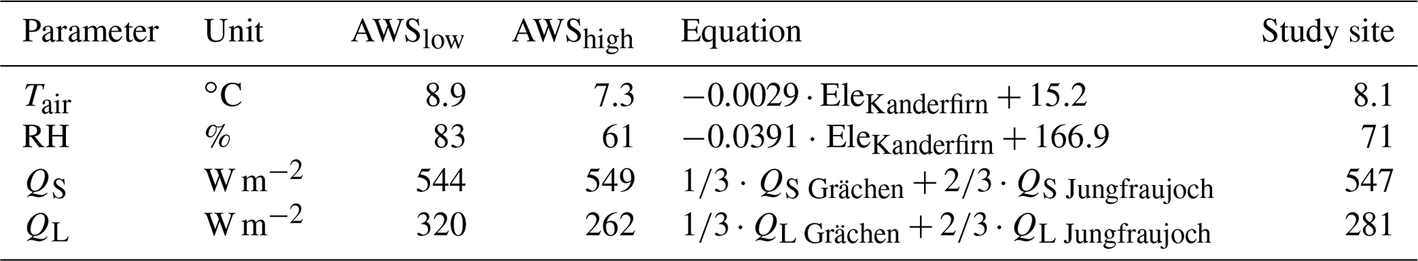
We rely on meteorological data for the processing of the radiometric UAV images (see Sect. 3.6) and for the debris thickness modelling (see Sect. 3.7). Two automatic weather stations operated by the WSL Institute for Snow and Avalanche Research (SLF), one at Fisistock (46.4715∘ N, 7.6739∘ E; 2160 m a.s.l.) and one at Gandegg (46.4293∘ N, 7.7606∘ E; 2710 m a.s.l.), are located 7 and 5 km away from the Kanderfirn and continuously measure air temperature and relative humidity. We calculated the mean air temperature and relative humidity for the period of the UAV surveys (13:00–15:00, CEST) and extrapolated the data from the two stations to the elevation of the study site (ca. 2460 m a.s.l.) using a simple linear regression model (Table 2). As the incoming shortwave and longwave radiation fluxes are not measured at these stations, we drew on data from two other weather stations, Grächen (46.1953∘ N, 7.8368∘ E; 1600 m a.s.l.) and Jungfraujoch (46.5476∘ N, 7.9854∘ E; 3570 m a.s.l.), which are located ca. 30 and 15 km away from the glacier and operated by the Swiss Federal Institute of Meteorology and Climatology (MeteoSwiss). We used the distance-weighted arithmetic mean to account for the varying distance between the glacier and both stations (Table 2).
Table 2Estimate of air temperature (Tair), relative humidity (RH), incoming shortwave radiation (QS) and incoming longwave radiation (QL) at the study site (ca. 2450 m a.s.l.) during the two UAV surveys (13:00–15:00, CEST) based on meteorological data from four weather stations in the vicinity of the glacier: Fisistock (2160 m a.s.l., AWSlow for Tair and RH), Gandegg (2710 m a.s.l., AWShigh for Tair and RH), Grächen (1600 m a.s.l., AWSlow for QS and QL) and Jungfraujoch (3570 m a.s.l., AWShigh for QS and QL). Data providers: Swiss Federal Office of Meteorology and Climatology (MeteoSwiss) and WSL Institute for Snow and Avalanche Research (SLF).
3.5 Photogrammetric processing
We used structure-from-motion (SfM) and multi-view-stereo (MVS) techniques to generate a visual orthophoto, thermal orthophoto and digital surface model (DSM) from the UAV imagery. The visual orthophoto served as the basis for the ice, snow and debris masks, and the thermal orthophoto served as the basis for the surface temperature and debris thickness maps (see Sect. 3.6 and 3.7). The DSM assisted the interpretation of the results.
We used only a subset of all acquired visual UAV images for the creation of the DSM and visual orthophoto to reduce the processing time. By selecting every eighth image, an overlap of 78 % could be achieved, guaranteeing still sufficient overlap in flight direction. The lateral image overlap, determined by the flight track distance (21 m), was about 85 %. All images taken during flight direction changes were excluded from the selection. A total of 101 visual images from both UAV surveys were used for the subsequent photogrammetric processing.
The radiometric JPG files captured by the TIR camera display a colour gradient adjusted to the measured temperature range. The measured temperature values themselves are not retrievable outside of proprietary FLIR software. They are calculated by the camera from the sensor signal (raw data) and corrected by applying an undisclosed proprietary algorithm based on the environmental parameters set prior to the capture. The colour gradient itself is useless for quantitative image analysis. To extract the raw data from the radiometric JPGs or to change the temperature correction settings after the acquisition, proprietary FLIR software packages are usually required (FLIR Systems, 2015; Teledyne FLIR, 2021b). This method has disadvantages, as these software packages are expensive and the algorithms used for temperature correction are not disclosed. We therefore drew on an open-source command-line application called ExifTool to retrieve the raw data from the radiometric images. ExifTool has been developed for reading, writing and manipulating image, video and audio metadata (Harvey, 2021). The raw data contain dimensionless 16-bit number values corresponding to the electronic signal readout of the microbolometer sensor (Minkina and Dudzik, 2009; Pour et al., 2019; Tattersall, 2021b). Accurate surface temperatures could then be calculated from the raw values (see Sect. 3.6). As the radiometric images are not geotagged, positional information were copied from the metadata of the visual images with equivalent timestamps using the ExifTool and R (R Core Team, 2019; Harvey, 2021). A few blurred images and those taken during changes in flight direction, takeoffs and landings were excluded from further processing. By selecting every fifth image, a sufficient overlap of ca. 80 % in flight direction was achieved. The overlap between images from parallel flight tracks was around 75 %. A total of 162 radiometric images from both UAV surveys were used for photogrammetric processing.
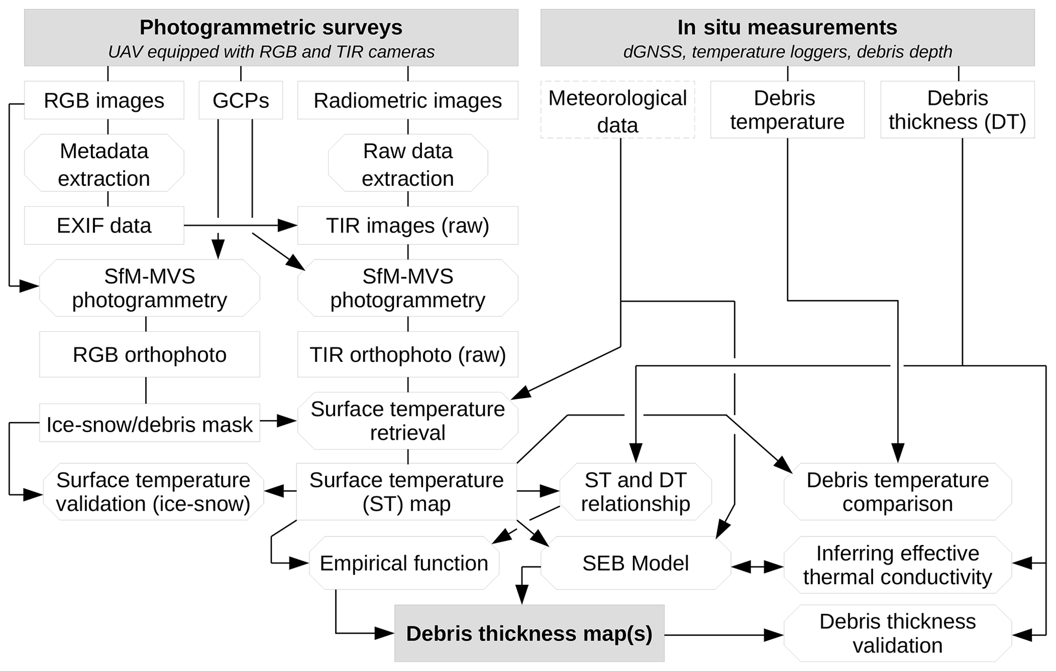
Figure 4Open-source workflow for the processing of visual and radiometric UAV imagery from glacial environments and the generation of accurate high-resolution surface temperature and supraglacial debris thickness maps.
For the photogrammetric processing of UAV imagery (from glacial environments) and the generation of accurate orthophotos and DSMs, both proprietary software (e.g. Kraaijenbrink et al., 2018; Bisset et al., 2022; Gök et al., 2023) and open-source software (e.g. Groos et al., 2019, 2022a) are available and have been successfully applied. We processed the selected visual and thermal images using the open-source software OpenDroneMap (ODM, version 2.9.2, https://opendronemap.org/, last access: 8 January 2024) with the application programming interface WebODM (version 2.2.0), following the general workflow described in Groos et al. (2019) and Groos et al. (2022a). Each of the 12 accurately measured visual GCPs (see Fig. 3 and Sect. 3.2) was referenced in five UAV images and passed to WebODM for georeferencing and accuracy optimisation of the DSM and visual orthophoto. The spatial resolution was set to the ground sampling distance (GSD). We used the default settings in WebODM and only changed the point cloud density and feature quality from medium to maximum (flag: pc-quality = ultra, feature-quality = ultra) to create a visual orthophoto and DSM (flag: dsm = true, dem-gapfill-steps = 5). From the thermal images, only a thermal orthophoto was computed using the same settings as described above. Eleven thermal GCPs were passed to WebODM as one thermal GCP (no. 12) was not visible in enough images.
For an independent assessment of the output of our complete open-source pipeline presented in Fig. 4, we processed the thermal images additionally with the established proprietary software Pix4Dmapper (Pix4D, 2021a). Processing was done with a high point density. The output resolution was set to GSD. By default, Pix4Dmapper adjusts pixel values when stitching images to create an aesthetically pleasing image. With the reflectance map option, the adjustment of the pixel values can be skipped to display the pixel values faithfully (Pix4D, 2021b). Since the radiometric values were of central interest, this option was used.
3.6 Surface temperature retrieval
The radiometric orthophotos computed with ODM and Pix4Dmapper contain dimensionless values corresponding to the electronic signal of the microbolometer sensor of the TIR camera. To obtain surface temperatures, the dimensionless values must be converted to the corresponding brightness temperature incident on the thermal camera. Additionally, environmental influences that lead to discrepancies between the actual thermodynamic temperature of the surface and the brightness temperature, which is measured by the thermal camera, must be corrected for (Minkina and Dudzik, 2009; Teledyne FLIR, 2016; Pour et al., 2019; Tattersall, 2019).
The conversion and correction was carried out with a simplified version of the “raw2temp” algorithm of the R package “Thermimage” (Tattersall, 2021a), which is based on the work of Minkina and Dudzik (2009). The output of the algorithm is the corrected surface temperatures in ∘C. It has been shown that the raw2temp algorithm computes surface temperatures very similar to those of several proprietary software packages (Tattersall, 2019), such as FLIR Tools (FLIR Systems, 2015) and FLIR Thermal Studio (Teledyne FLIR, 2021b). The algorithm firstly calculates an atmospheric transmission factor. Secondly, it calculates the portion of the signal attributable to the thermal radiation flux of the atmosphere and the thermal radiation flux reflecting off the investigated surface. Using the atmospheric transmission, emissivity and the interfering radiation fluxes, the surface temperature is calculated from the raw signal.
3.6.1 Atmospheric correction
To correct for the atmospheric influence on the radiometric measurements, information on the height of the air column between the glacier surface and sensor is important. The flight height was therefore taken into account. Moreover, knowledge of the meteorological conditions at the study site during the subsequent UAV surveys is essential. As a rough estimate, we calculated the mean air temperature (Tair) and relative humidity (RH) at the study site during the UAV surveys using data from two nearby weather stations and a simple linear regression model (see Sect. 3.4 and Table 2). Following the procedure of Tattersall (2021a), water vapour pressure (Pwv) was estimated from air temperature and relative humidity:
It served for the determination of an atmospheric transmission correction factor (τ) (Tattersall, 2021a):
where hUAV is the flight height of the UAV. An overview of the different atmospheric attenuation constants (provided by FLIR within the metadata) is given in Table 3. The TIR radiance of the atmosphere (radatm) is calculated in raw units (Tattersall, 2021a):
from which the fraction of the atmosphere's thermal radiation of the radiation flux arriving at the sensor (radatm.attn) is determined using the atmospheric correction factor (τ) and the thermal emissivity (ε) of the surface material (debris or ice/snow):
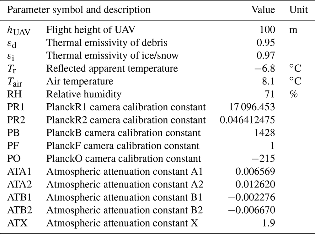
Table 3Parameter values used for the calculation of surface temperatures from the TIR camera signal. The determination of relative humidity and air temperature is outlined in Sect. 3.4 and Table 2. Flight height is known from flight planning. Surface emissivity values were taken from the literature (Salisbury and D'Aria, 1992; Rivard et al., 1995; Kraaijenbrink et al., 2018; Mineo and Pappalardo, 2021), and all attenuation and calibration constants were read from the thermal image Exif data.
3.6.2 Reflected apparent temperature correction
The algorithm of Tattersall (2021a) further corrects for thermal radiation from the ambient air or surrounding objects that is reflected off the investigated surface. If surface reflectance is higher than 0 (ε<1), the reflected thermal radiation influences the surface temperature measurement (Cronholm, 2002; Minkina and Dudzik, 2009).
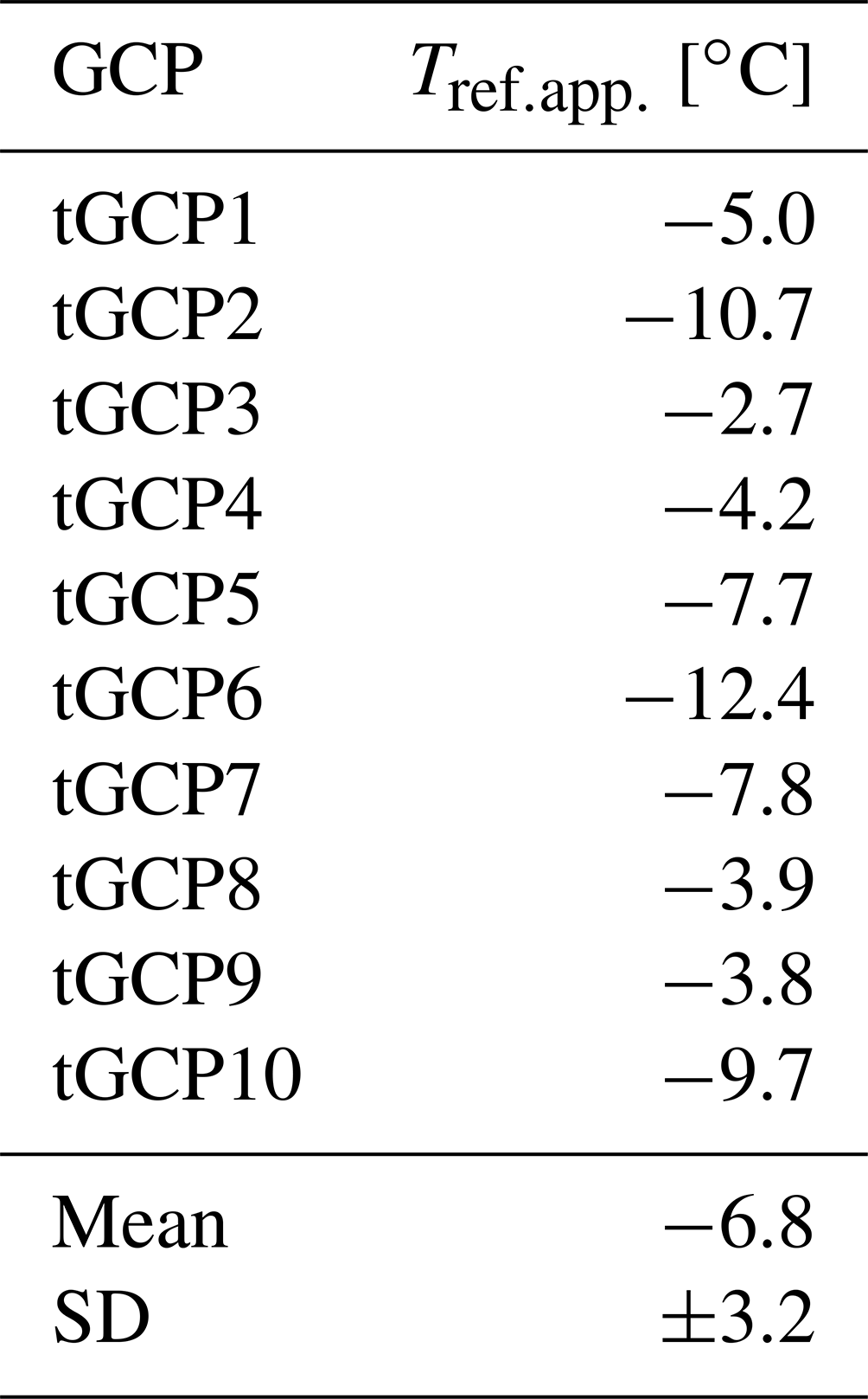
A suggested method to measure the reflected apparent temperature, which is the temperature ascribed to the radiation reflected by the investigated surface, is to use crinkled and reflattened aluminium foil. It is laid on the target surface as a highly reflective and diffuse reflector of ambient radiation. By measuring its brightness temperature with emissivity set to 1, where emissivity itself has no effect on the measurement, the reflected apparent temperature can be approximated (e.g. Cronholm, 2002; Baker et al., 2019). The thermal GCPs served as a simple diffuse reflector. Hence, the temperature of each thermal GCP was extracted from the thermal orthophoto calculated as outlined in this section but with emissivity set to 1. The mean of the temperature readings (−6.8 ∘C) of all 10 thermal GCPs visible in the thermal orthophoto was taken as the reflected apparent temperature for surface temperature retrieval. The reflected apparent temperature for each GCP is listed in Table 4.
Table 4Reflected apparent temperature () derived from the brightness temperature (ε=1) calculated for the centre of each thermal GCP (see Sect. 3.6.2).
Based on the reflected apparent temperature (Tr) and following Tattersall (2021a), the TIR radiance reflected by the surface (radrefl) is calculated in raw units,
from which its fraction of the thermal radiation flux incident on the sensor (radrefl.attn) is calculated as
3.6.3 Emissivity correction and surface temperature determination
Lastly, the algorithm corrects for emissivity (ε). Emissivity is used to characterise materials by how effectively they emit energy in the form of thermal radiation. It is expressed as a value between 0 (perfect reflector) and 1 (perfect emitter/black body). Every real object has an emissivity lower than 1 and therefore emits less radiation than a hypothetical perfect emitter at the same temperature. Hence, if emissivity is not adjusted for, a TIR camera would measure a surface temperature lower than the actual surface temperature of the object (Avdelidis and Moropoulou, 2003; National Physical Laboratory, 2021; Teledyne FLIR, 2021a). For this correction step, the assumed emissivity of the debris layer is needed (Pour et al., 2019; Tattersall, 2021b; Minkina and Dudzik, 2009).
The emissivity of a given surface depends on the material, surface properties, measurement temperature, measurement angle and measurement wavelength (Salisbury and D'Aria, 1992; Rivard et al., 1995; Mineo and Pappalardo, 2021; National Physical Laboratory, 2021). Its estimate is therefore a source of uncertainty. As laboratory measurements were beyond the scope of this study, we relied on values from the literature. The debris-covered area on the Kanderfirn is mainly made up of limestone and marly shales. Locally, smaller amounts of ferrous limestone and igneous rock are present. The latter lithologies were neglected for the emissivity estimate due to their scarcity.
Only limited literature is available on the emissivity of rock materials. Rivard et al. (1995) measured emissivities of around 0.95 in the wavelength of 7.5–13 µm for different limestone samples. Mineo and Pappalardo (2021) also measured emissivities of around 0.95 for limestone and similar values for other calcareous rocks in the same wavelength. Hence, we assumed an emissivity of 0.95 for the debris cover. However, the emissivity of the debris cover on the Kanderfirn may differ from this estimate. For surface temperature calculation of the clean-ice and snow-covered areas, we used an emissivity of 0.97 (e.g. Salisbury and D'Aria, 1992; Kraaijenbrink et al., 2018). For simplicity, this emissivity was also applied to the few and dispersed stream and pond surfaces, which are hard to differentiate from the bare ice surfaces.
Along with the atmospheric transmission and radiation fluxes described above, the emissivity (either for debris or ice/snow) is used in the algorithm of Tattersall (2021a) to calculate a raw unit equivalent to the actual surface temperature (rads) from the camera signal values (rad),
from which the surface temperature (Ts) in ∘C is then determined by applying various calibration constants extracted from the metadata of the TIR camera (see Table 3).
3.6.4 Snow and ice masking and GCP temperature correction
To delineate snow and ice from debris, a mixed-method approach was used. Based on the visual orthophoto, a polynomial thresholding approach, as proposed by Burton-Johnson and Wyniawskyj (2020), was used. The method exploits the fact that the red-to-blue-band ratio of rock is higher than that of snow and that the ratio increases with reflectance. Subsequently, both 300 training pixels of rock debris and 300 training pixels of snow and bare ice were used to fit a second-order polynomial curve that separates the classes as a function of red-to-blue-band ratio and reflectance. Using this polynomial threshold, a mask classifying pixels into either rock debris or snow and ice was derived. Some manual adjustments were done to the mask, which include cluster–size-dependent smoothing of the mask, manual corrections for misclassifications in the area of larger snow patches, manual reclassification of wrongly classified ice cliffs and bright rocks, and resampling of the mask to the pixel size of the thermal orthophoto. In the areas classified as snow or ice, surface temperatures were calculated using an emissivity of 0.97; in all other areas, an emissivity of 0.95 was applied.
Lastly, the thermal GCPs wrapped in aluminium foil displayed unrealistically low temperatures as their low emissivity is not accounted for in the correction. The temperature values of the affected areas (< 0.75 m2 for each GCP) were therefore replaced by the surrounding values using the inverse distance weighting approach.
3.6.5 Accuracy assessment of surface temperatures
Since the surface temperature of ice and snow on a summer day is expected to be close to the melting point (0 ∘C), the ice and snow areas surveyed with a UAV can help to assess the accuracy of the mapped surface temperatures (Kraaijenbrink et al., 2018). However, ice and snow surfaces that are partially covered with dark cryoconite are likely to have surface temperatures slightly exceeding 0 ∘C. We evaluated the deviation of the surface temperature from 0 ∘C over the debris-free and snow-covered areas of the test site on the Kanderfirn using the created ice–snow mask.
To evaluate the calculated debris surface temperatures and detect possible biases, the means of the debris temperature logger readings during the two flights were compared to the corresponding temperature values in the corrected thermal orthophoto. For the position of each logger, the surface temperature was extracted from the corrected thermal orthophoto. The area mean of a 3×3 pixel window centred around the logger position was used to account for uncertainties in the thermal orthophoto and temperature logger position.
3.7 Debris thickness mapping
A supraglacial debris thickness map can be derived from a corrected thermal orthophoto for areas with a debris thickness of less than ∼ 0.5 m using either a local empirical relationship between debris thickness and surface temperature or an inverted glacier surface energy balance model, provided that the thermal imagery was collected at a time when the debris surface temperature was sufficiently heterogeneous (e.g. Mihalcea et al., 2008a, b; Foster et al., 2012; Juen et al., 2014; Rounce and McKinney, 2014; Groos et al., 2017; Rounce et al., 2018, 2021). We explored both approaches following the procedure below (see Fig. 4).
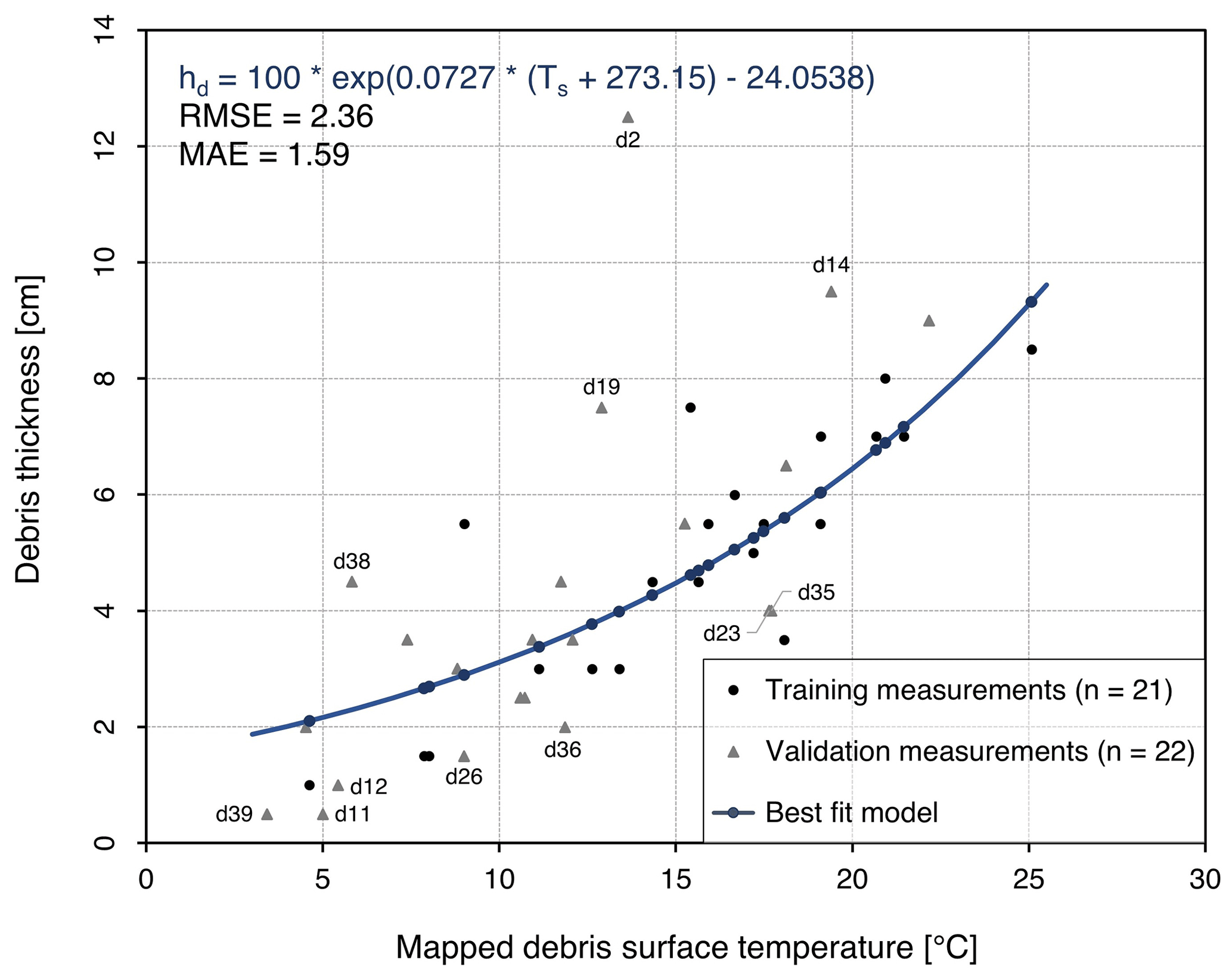
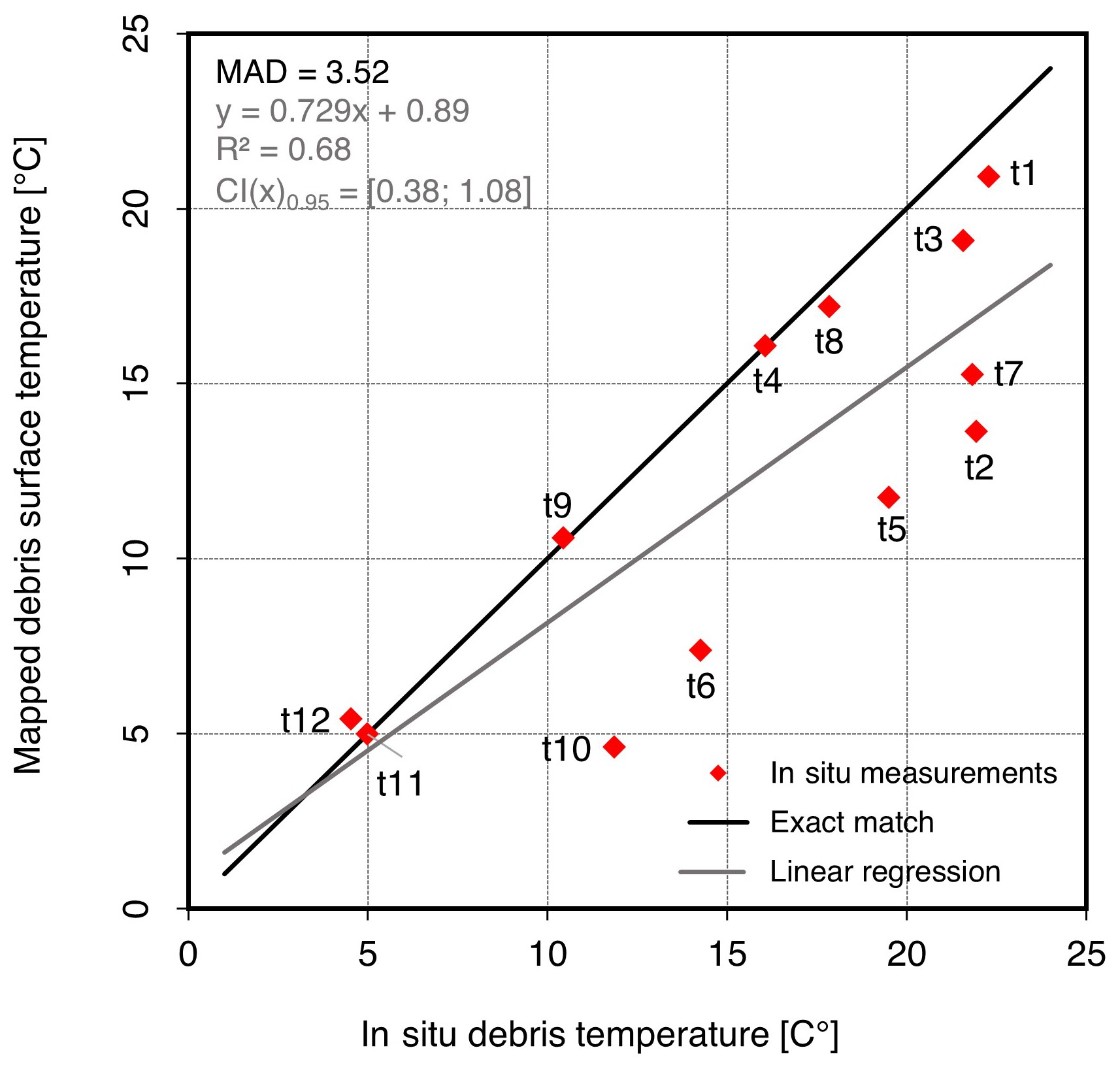
Figure 5Empirical relationship between measured debris thickness and mapped debris surface temperature. The best-fit model served for the extrapolation of the point data and the computation of a debris thickness map. Validation measurements that deviate considerably from the best-fit model are labelled.
3.7.1 Empirical method
A site- and time-specific exponential function with two fitting parameters is suitable to predict debris thickness from surface temperature (e.g. Mihalcea et al., 2008b). The fit is iteratively compared to the measured data using different starting values for the fitting parameters, which are selected using non-linear least squares (e.g. Mihalcea et al., 2008a, b; Juen et al., 2014; Groos et al., 2017). To enable the point-wise comparison of measured debris thickness and mapped surface temperature, we extracted the surface temperature from the corrected thermal orthophoto at the location of each in situ debris thickness measurement using a 3×3 pixel matrix. The 43 measurement pairs were randomly split into a training and validation dataset. On the basis of the training dataset, an empirical best-fit model was calculated using the “debrisThicknessFit” function from the R package “glacierSMBM” (Groos et al., 2017; Groos and Mayer, 2017):
where hd is the predicted debris thickness (m) and Ts is the debris surface temperature (K). The best-fit model served for the extrapolation of the point data and the computation of a debris thickness map using the “debrisThicknessEmp” function from the same R package. Half of the debris thickness measurements (n=22) were considered for the validation.
3.7.2 Surface temperature inversion method
Surface energy balance models of varying complexity have been developed to predict ice melt beneath supraglacial debris using meteorological data and information on site-specific debris properties (e.g. Nicholson and Benn, 2006; Evatt et al., 2015). If solved for debris thickness, these models enable the calculation of debris thickness from surface temperature and the residual of the considered energy fluxes (e.g. Foster et al., 2012; Rounce and McKinney, 2014; Schauwecker et al., 2015; Groos et al., 2017; Rounce et al., 2021). We implemented and tested the theoretical sub-debris ice melt model of Evatt et al. (2015, Eq. 46) as it has been proven to reproduce the characteristic features of the empirical Østrem curve (Østrem, 1959):
where QM is the sub-debris ice melt rate (m s−1), hd is the debris thickness (m), γ is a wind speed attenuation constant (234 m−1), and the other terms are (Evatt et al., 2015, Eqs. 41–45)
A summary of the units and values of the individual parameters and constants is provided in Table 5. Please refer to the original publication for more information on the derivation of the individual equations. The surface temperature (Ts) of the debris layer is
After rearrangement, this function can be used to derive debris thickness from surface temperature and meteorological data:
To assess the model uncertainties related to the meteorological input parameters (i.e. air temperature, incoming shortwave and longwave radiation, wind speed; see Table 2) and debris properties (i.e. albedo, effective thermal conductivity), we performed a simple sensitivity analysis by varying the individual model parameters within the maximum range of expected uncertainties (Tair: ±2 ∘C; QS and QL: ± 50 W m−2) or within the range of plausible values (um: 2.0–4.0 m s−1; αd: 0.07–0.27; κ: 0.50–1.50 W m−1 K−1). Since the thermal conductivity is a sensitive parameter in sub-debris ice melt models (e.g. Steiner et al., 2021) that has a large impact on the modelling of relatively thin debris (< 10 cm), which is predominant on the Kanderfirn and many other glaciers, we used this parameter for model calibration. Conversely, this allows the effective thermal conductivity of a debris layer to be estimated if its thickness and surface temperature are known.
Table 5Parameter values used for the surface energy balance model (Eq. 17). The first 11 parameter values are site-specific (see Sect. 3.4 and 3.6.3). The albedo of the debris layer of the Kanderfirn was estimated using the glacier albedo map of Naegeli et al. (2019). The effective thermal conductivity was calibrated against in situ observations, and the thermal emissivity of the debris layer was estimated (see Rivard et al., 1995; Mineo and Pappalardo, 2021). The last six parameters take non-site-specific values. Parameter values adopted from the original publication are indicated with an asterisk (see Evatt et al., 2015).
4.1 Measured debris thickness and temperature
During the two UAV surveys on 28 September 2021, the mean debris temperature measured at 12 locations (Fig. 1) at a depth of ca. 0.5–1.0 cm varied spatially and ranged from 4.5 to 22.3 ∘C (Table A2 and Fig. 6). The thickness of the supraglacial debris layer measured manually at 43 points on the Kanderfirn (Fig. 1) ranges from less than 1 cm up to 13 cm (Table A1). Individual boulders scattered over the debris-covered glacier area are more than 50 cm high, but they were not measured or mapped explicitly. The average of the measured debris thickness is 4.6 cm and the median is 4.5 cm. The distribution of the point measurements has a positive skew, indicating that very thin debris thicknesses (< 5 cm) predominate (Fig. 7).
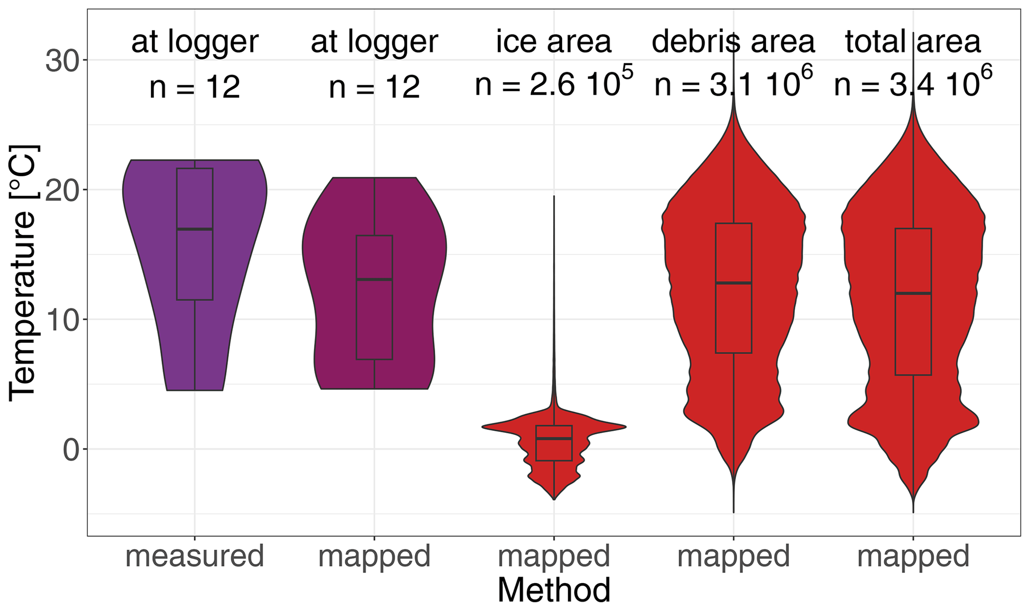
Figure 6Distribution of the 12 in situ debris temperature measurements at a depth of ca. 0.5–1.0 cm below the surface of the debris layer (Fig. 1) and distribution of the mapped surface temperatures (Fig. 10) at the location of the temperature loggers, across the debris-free area, across the debris-covered area and across the total survey area. n indicates the number of loggers or the number of considered pixels.
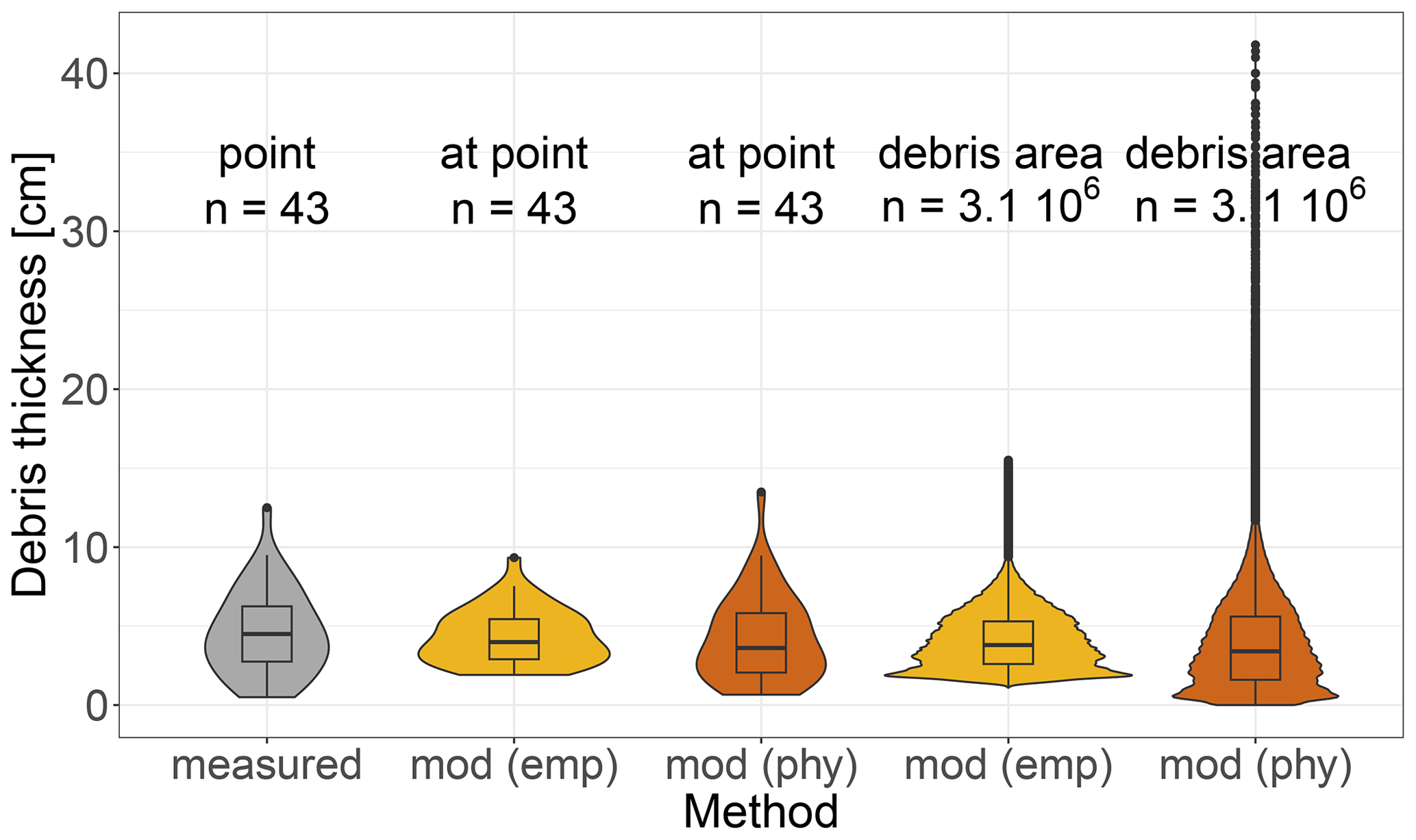
Figure 7Distribution of the 43 in situ debris thickness measurements (see Fig. 1) and distribution of the debris thicknesses (see Figs. 12 and 15g) at the measurement positions and across the surveyed debris-covered area predicted with the empirical (emp) and physical (phy) model (mod). n indicates the number of measurements or the number of considered pixels.
4.2 Positional accuracy of visual and thermal orthophotos
The positional accuracy of the generated orthophotos was assessed by determining the XY error between the GCPs as measured with the dGNSS and their position on the orthophoto. For the visual orthophoto, the accuracy obtained at 12 GCPs (Fig. 1) ranges from 5 to 21 cm (Table A3). The accuracy at most of the GCPs is similar to or smaller than the positional uncertainty of the differential GNSS measurements itself. The RMSE as a measure for the overall positional accuracy is 13 cm. For the thermal orthophoto, the accuracy obtained at 11 GCPs ranges from 5 to 39 cm (Table A4). The accuracy at the individual GCPs is similar to the positional uncertainty of the differential GNSS measurements. The RMSE of 17 cm is slightly higher than that of the visual orthophoto and only slightly more than the GSD of 13 cm. The positional accuracy of the thermal orthophoto produced with ODM is similar to that of Pix4D.
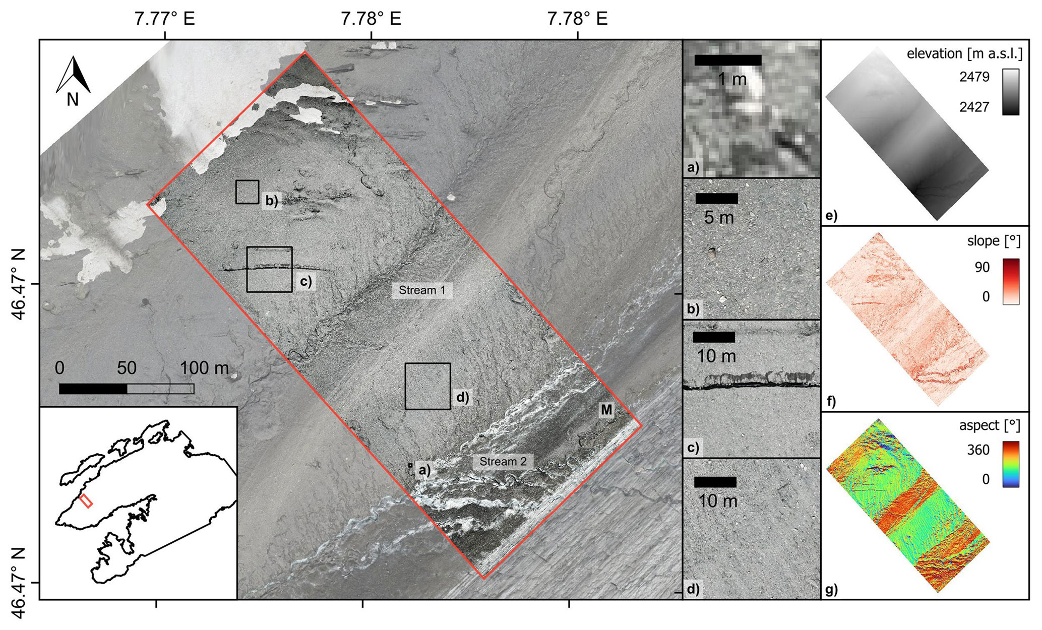
Figure 8(a) High-resolution visual orthophoto of the glacier area surveyed on 28 September 2021, comprising clean ice, debris-covered ice (b, d), snow deposits from avalanches, crevasses (c, black line), ice cliffs (c, dark greyish areas to the north of the crevasse) and meltwater channels. Inset (e) shows the topography, (f) the slope and (g) the aspect of the study area. “M” indicates the medial moraine mentioned in the text. Background: UAV-based orthophoto from 14 September 2021.
4.3 Surface characteristics and topography of the debris layer
The high-resolution orthophoto and DSM (GSD =5 cm) cover a glacial area of ca. 6.5 ha (170×390 m) and include clean ice, debris-covered ice, avalanche deposits, crevasses, ice cliffs and meltwater channels (Fig. 8). Most of the surveyed area is covered with debris. Clean ice can be found in the southeastern part of the surveyed area and snow deposits from avalanches in the northwestern part below the south face of the Blüemlisalp. One meltwater channel runs more or less parallel to the debris–ice transition area, and the other one forms a small valley, separating the debris-covered area into two elevated parts. The height difference between the lowest point of the meltwater channel and the highest point of the debris-covered area is about 50 m. Ice cliffs occur close to the central stream (labelled with “Stream 1”) and in both elevated debris-covered areas. Larger crevasses are restricted to the area northwest of the central stream. In the southeastern corner of the surveyed area, the lower part of a medial moraine (labelled with “M” in Fig. 8) that is crosscut and dispersed by Stream 2 can be seen (Fig. 8; for a better overview see Fig. 11 in Groos et al., 2019).
4.4 Difference between measured and mapped debris temperatures
The cross-comparison shows that the measured debris temperatures and mapped surface temperatures agree relatively well (Fig. 9). The coefficient of determination (R2) is 0.68. The difference between the measured and mapped temperatures ranges from −8.3 to 0.9 ∘C. At five points, the absolute deviation exceeds 6 ∘C. However, the absolute deviation at the other points is consistently less than 2.5 ∘C and in most cases less than 1 ∘C. The mean absolute difference (MAD) is 3.5 ∘C.
4.5 Spatial variations in glacier surface temperature
The corrected thermal orthophoto has a GSD of 13 cm and covers an area of about 6.5 ha (Fig. 10). The differences (see Fig. B1) between the surface temperature derived from the thermal orthophoto generated with the open-source software (ODM) and the one derived from the thermal orthophoto generated with the established proprietary software (Pix4Dmapper) is negligible (0.2 ± 1.2 ∘C). Small-scale deviations originate from the imperfect co-registration of both maps and are not further discussed here. More interesting is the prominent large-scale, stripe-like pattern tracing the flight tracks, possibly caused by interference with solar radiation in the southeastern direction of flight. Why the signal is imprinted only in one of the two thermal orthophotos is not clear. Since the deviations are overall very small and have little influence on the final debris thickness map, the spatial surface temperature variations are illustrated only for the thermal orthophoto that was obtained through the photogrammetric processing of the radiometric images with ODM. Spatially, the mapped surface temperatures vary between −5 and 32 ∘C, but most pixel values are between 0 and 25 ∘C (Fig. 6). Surface temperatures are lowest on the snow patches and highest in the elevated debris-covered area below the Blüemlisalp south face. Due to their much lower temperatures, small-scale features such as crevasses, ice cliffs and supraglacial meltwater channels are clearly visible in the map (Fig. 10c). Characteristic stripe-like patterns in the debris-covered area that are not recognisable in the visual orthophoto become apparent in the thermal orthophoto (Fig. 10d).
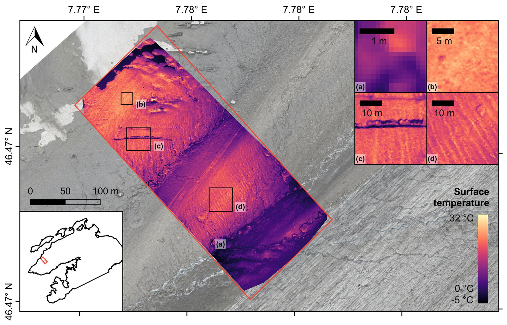
Figure 10Corrected thermal orthophoto showing the surface temperature of the surveyed glacier area at about 14:00 on 28 September 2021. The four highlighted sections (a, b, c, d) are the same as in Figs. 8 and 12. Detail (a) illustrates the spatial resolution, detail (b) shows a debris-covered area with relatively high surface temperatures, detail (c) includes a crevasse and an ice cliff, and detail (d) is an example of small-scale debris surface temperature variations. Background: UAV-based visual orthophoto from 14 September 2021.
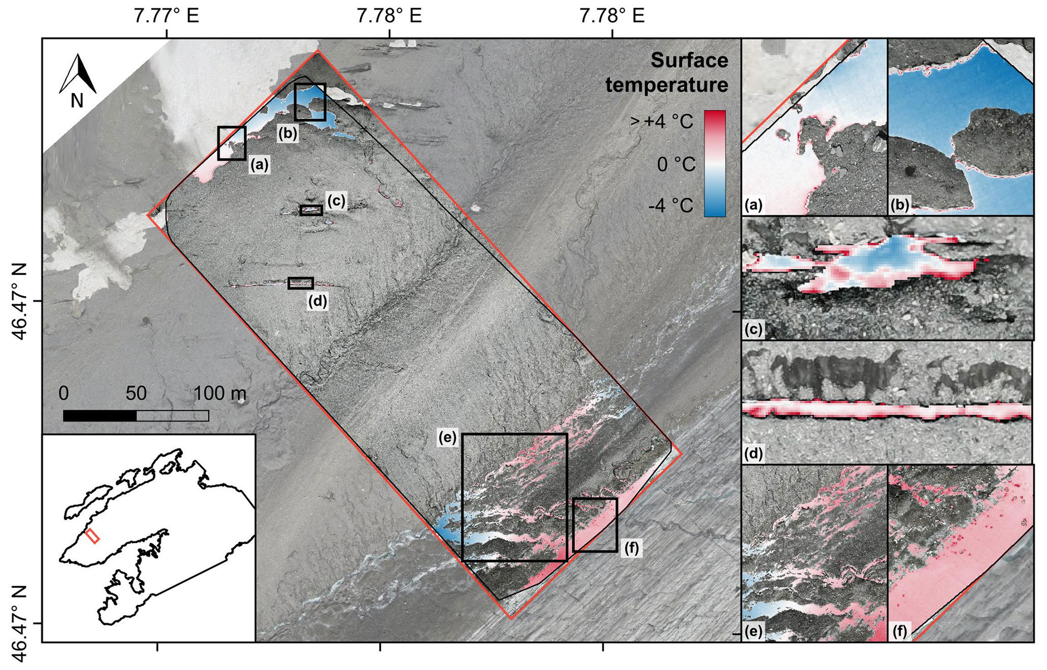
Figure 11Surface temperatures of snow and bare ice areas derived from the thermal orthophoto. These areas serve the assessment of the accuracy and plausibility of the mapped surface temperatures. The enlarged map sections are discussed in the text. Background: UAV-based visual orthophoto from 14 September 2021.
Since snow and ice surfaces can be expected to be relatively close to the melting point on afternoons during the ablation season, such areas can serve as a reference for assessing the accuracy and plausibility of mapped glacier surface temperatures. Throughout the entire surveyed glacier area, the deviation of the snow and ice surface temperatures from 0 ∘C is less than the measuring accuracy of the TIR camera (Fig. 11). The surface temperatures of debris-free ice ranges from −0.9 to 1.8 ∘C (interquartile range; see Fig. 6). The surface temperatures of the larger ice cliffs in the centre of the survey area (Fig. 11a, b) are relatively close to the melting point (Fig. 11c, d). Positive deviations larger than 3 ∘C are restricted to the edges of the snow patches and ice surfaces (Fig. 11a–d). A fraction of the snow patch in the northeastern part of the survey area shows surface temperatures close to −4 ∘C (Fig. 11b). Moreover, a general tendency towards higher deviations from the melting point can be observed towards the edges of the thermal orthophoto (Fig. 11). However, the moderate deviation of the surface temperature from the melting point in the debris-free area (0.6 ± 2.0 ∘C) proves overall the suitability of the presented methodology for mapping glacier surface temperature in high resolution and with adequate accuracy.
4.6 Spatial variations in supraglacial debris thickness
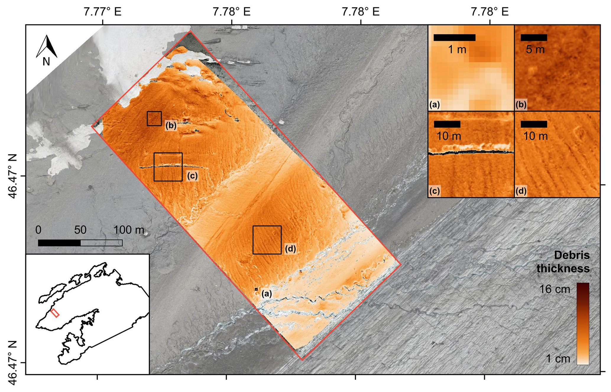
Since the supraglacial debris thickness maps were derived from the corrected thermal orthophoto, spatial variations in debris thickness and surface temperature correlate with each other (cf. Figs. 10 and 12). The debris thickness predicted with the empirical model shows a high spatial variability and ranges from around 1 up to 16 cm (Fig. 7). The RMSE of the empirical model calculated on the basis of the in situ measurements is 2.4 cm (using only the validation points; see Fig. 5) or 1.3 cm (using all data points; see Fig. 16), and the mean absolute error (MAE) is 1.6 cm. In general, the debris layer becomes thicker towards the glacier margin below the south face of the Blüemlisalp (Fig. 12b). Besides this, the debris layer appears to be relatively thick (ca. 5–10 cm) in the elevated area between the parallel supraglacial meltwater streams (Fig. 12d). Close to the bare-ice surface, the debris cover tends to be very thin (< 2 cm), apart from the supraglacial moraine at the debris–ice margin (labelled with “M” in Fig. 10). Individual spots of higher debris thickness indicate larger rocks or debris cones. A remarkable feature is the stripe-like patterns that are clearly visible in the debris thickness map (Fig. 12c, d) but poorly visible in the visual orthophoto (Fig. 8). The underlying mechanism of formation is unknown, but as the alternating stripes of thicker and thinner debris run parallel to the slightly inclined slopes, we assume that they are the result of frost sorting or rain- and meltwater drainage during the ablation season.
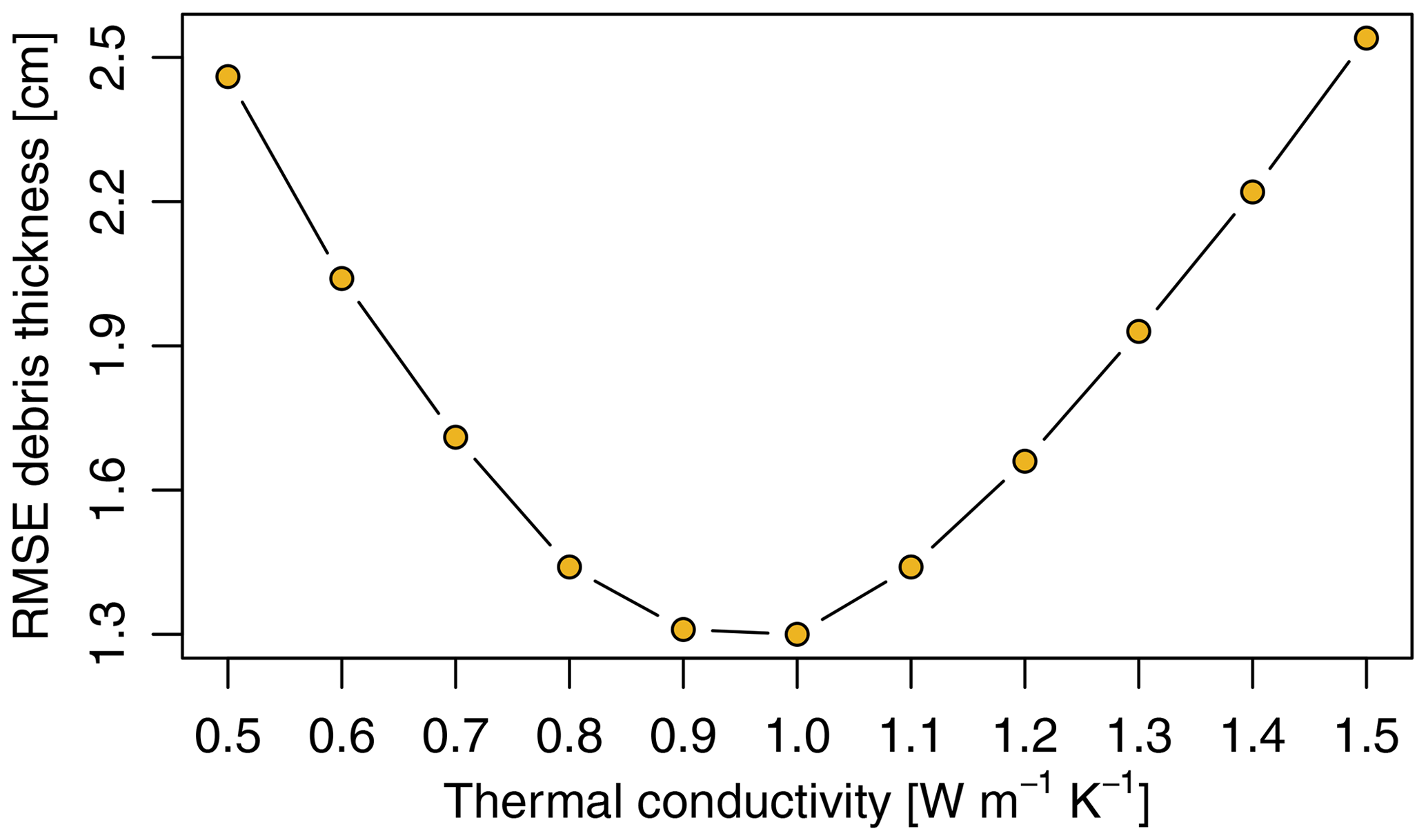
The range of debris thickness predicted with the inverse surface energy balance model depends on the parameter settings. The results of the sensitivity analysis suggest that the effective thermal conductivity of the debris layer and the wind speed above the debris layer are the most critical parameters in the model (Fig. 13). While the wind speed and other tested parameters affect mainly the prediction of debris thicknesses greater than 10 cm, the effective thermal conductivity is a crucial parameter for the accurate thickness estimation of relatively thin debris (Figs. 13 and 14). The greater the thermal conductivity, the thicker the debris (Fig. 15). Within the plausible range of potential thermal conductivities for a supraglacial debris layer (0.5–1.5 W m−1 K−1), the mean difference between the modelled and observed debris thickness varies between 1.3 and 2.5 cm. The model run with the smallest RMSE (1.3 cm) predicts a thermal conductivity in the order of 1.0 W m−1 K−1 for the debris layer on the Kanderfirn (Fig. 16). The remaining unexplained variance points to uncertainties originating from the energy balance model itself, from the estimated model parameters (and their spatial variability) and from the surface temperature map.
The debris thickness maps produced with the two different models (empirical and physical) agree well. They are generally very similar in terms of spatial patterns (Fig. 15). However, thickness deviations of up to ±2 cm are visible in some areas (Fig. C1). The intercomparison of the distribution of measured and modelled debris thicknesses indicates that the physical model performs better than the empirical models in terms of predicting very thin and relatively thick debris (Fig. 7). Moreover, the maximum debris thickness predicted with the physical model is about 40 cm. It therefore much better reflects the height of individual boulders that are spread across the debris-covered area.
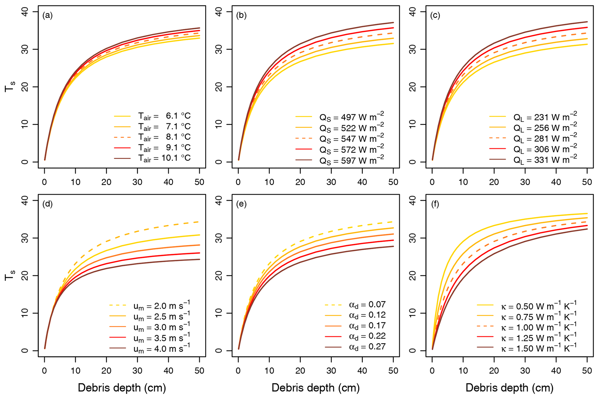
Figure 13Sensitivity of the inverse surface energy balance model with respect to the expected maximum range of uncertainty and spatio-temporal variability of six essential input parameters: (a) air temperature (Tair), (b) incoming shortwave (QS) and (c) longwave radiation (QL), (d) wind speed (um), (e) debris albedo (αd), and (f) effective thermal conductivity (κ) of the debris layer. The dashed lines represent the model run with the parameter values provided in Table 5 and used for Figs. 14g and 15g.
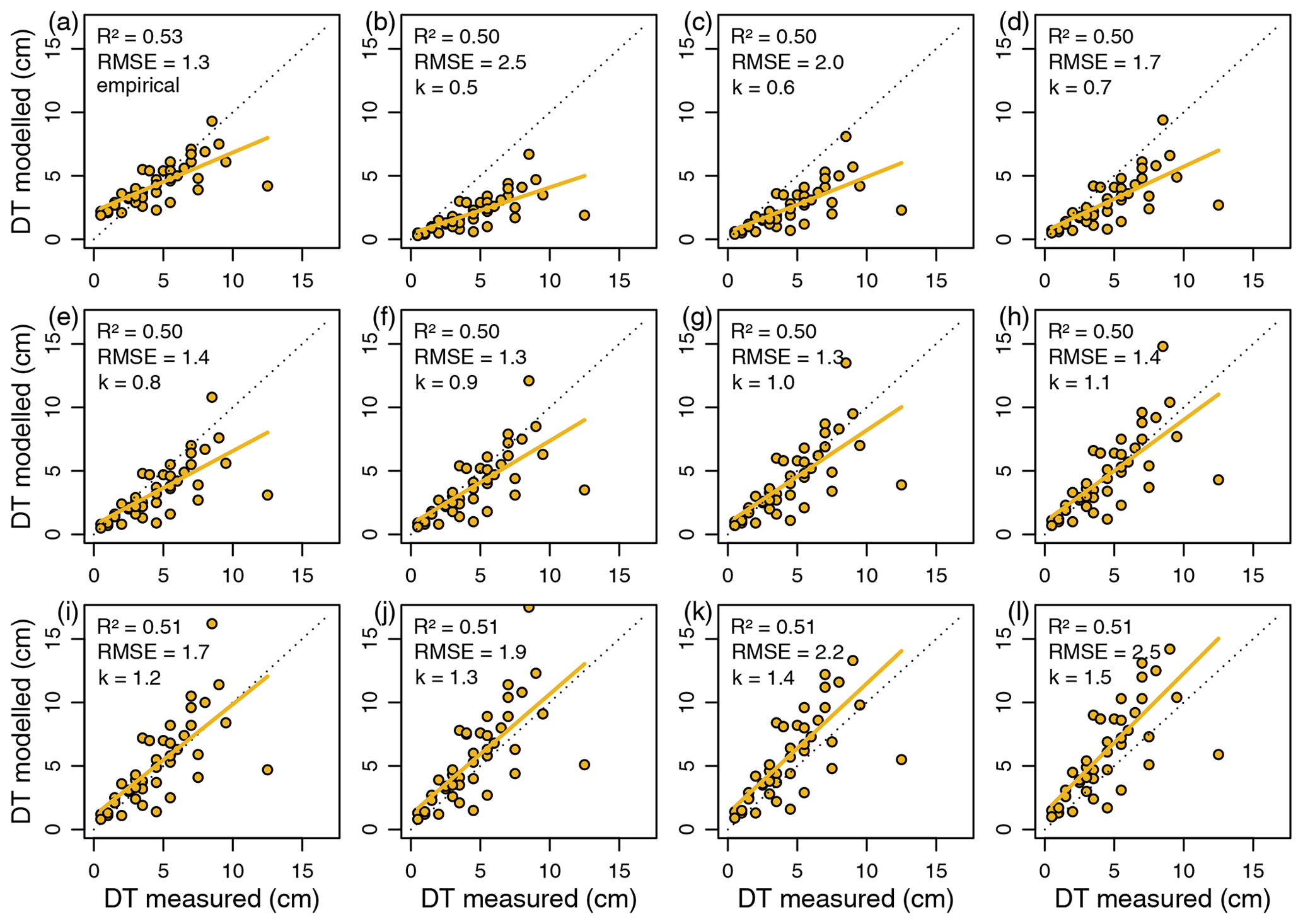
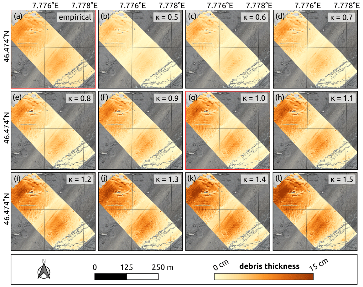
Figure 15Impact of thermal conductivity on the spatial distribution of supraglacial debris thickness. The debris thickness maps were calculated from the corrected thermal orthophoto for different thermal conductivities () using the inverted glacier surface energy balance model (Eq. 17) with the parameter values provided in Table 5. Note that the distributed debris thickness modelling with a thermal conductivity (k) of 1.0 W m−1 K−1 (red frame) shows the highest agreement with the in situ measurements and the empirical map (red frame).
The aim of the following discussion is to (i) outline suitable times and conditions for thermal imaging of supraglacial debris, (ii) illustrate improvements and best practices for accurate UAV-based thermal imaging in high-mountain environments, (iii) shed light on the sensitivity and limitations of the applied debris thickness models, and (iv) elaborate on the scalability of the UAV-based mapping approach.
5.1 Suitable times and conditions for thermal imaging of supraglacial debris
In terms of supraglacial debris thickness mapping, the timing of the acquisition of thermal images matters as the strength of the correlation between surface temperature and debris thickness depends on the time of day, meteorological conditions and debris properties. The large range and high spatial heterogeneity of debris surface temperatures on the Kanderfirn during the two subsequent thermal UAV surveys in the early afternoon on 28 September (see Figs. 6 and 10) facilitated the generation of accurate high-resolution debris thickness maps. Favourable for the surface temperature mapping was probably the moderate insolation due to the lower solar altitude at the end of the ablation season and the presence of altostratus or cirrostratus clouds, which reduced the likelihood that the surface of thicker debris (> 10 cm) became isothermal (e.g. Herreid, 2021). Based on the analysis of thermal orthophotos from different times of the day, Bisset et al. (2022) found that the maximum spatial surface temperature variance of the debris layer on Llaca Glacier in the Peruvian Alps was reached at midday. The authors therefore also concluded that midday to early afternoon is a suitable time for UAV-based thermal imaging and debris thickness mapping. However, Herreid (2021) and Aubry-Wake et al. (2023) pointed out that the surface of a thick debris layer may become isothermal during the hottest hours of a clear summer day. Morning hours seem in general unfavourable for debris thickness mapping as surface temperatures rise quickly and have a distinct terrain bias at this time of day (Gök et al., 2023). Days with partial cloud cover have the disadvantage that spatial surface temperature variations caused by shadows of fast-moving clouds must be corrected for when processing and analysing the radiometric images. While clear summer days seem to provide acceptable conditions for UAV-based mapping of thin debris, overcast days are probably best suited for deriving supraglacial debris thickness variations from mapped surface temperatures in general. Although the nighttime operation of UAVs in glacierised mountain environments is difficult to realise, it might be worthwhile to explore the potential of thermal imaging at night – when thermal radiation emitted from a supraglacial debris layer may be well related to its thickness – for the mapping of thick debris (Herreid, 2021; Aubry-Wake et al., 2023).
5.2 Accuracy of UAV-based thermal imaging
Since accurate and consistent surface temperatures are the prerequisite for reliable debris thickness mapping, radiometric thermal images collected with UAVs must be corrected for the effects of inherent sensors biases, thermal drift, atmospheric impacts, reflected thermal radiation and spatially varying emissivity (e.g. Ribeiro-Gomes et al., 2017; Kraaijenbrink et al., 2018; Virtue et al., 2021; Bisset et al., 2022; Gök et al., 2023). Low-cost uncooled microbolometers that are commonly used in UAV thermography are notoriously sensitive to changing atmospheric and environmental conditions. Temperature fluctuations of the camera housing, lens or sensor, caused for example by changes in wind speed or air temperature, lead to a disequilibrium between the sensor and ambient air, which may alter the surface temperature measurement. TIR cameras, such as the FLIR Vue Pro R 640 used in this study and by Bisset et al. (2022), perform a flat field correction using the closed shutter at power-up and periodically during operation (the exact procedure is not disclosed by the manufacturer) to compensate partially for the thermal drift during operation. However, the internal sensor calibration does not necessarily guarantee accurate surface temperature measurements. Gök et al. (2023) for example experienced considerable problems with the internal flat field correction of the FLIR Tau2, and Kraaijenbrink et al. (2018) observed a mean sensor bias in the order of 7 ∘C for the senseFly thermoMAP.
There are different options to assess the accuracy and plausibility of mapped glacier surface temperatures. While debris-free glacier surfaces are suitable to assess the overall accuracy of mapped ice and snow temperatures, independent measurements are necessary to validate the mapped debris surface temperatures. In the absence of independent debris (surface) temperature measurements, such as in the study by Gök et al. (2023), possible biases or shifts in the UAV-based debris surface temperature recordings might be overlooked. Independent and accurate ground-based measurements of the surface temperature of varying supraglacial debris thicknesses can be performed with a handheld TIR radiometer (Kraaijenbrink et al., 2018; Bisset et al., 2022). However, ground-based radiometric measurements are also subject to uncertainties (Aubry-Wake et al., 2015, 2018; Ribeiro-Gomes et al., 2017; Herreid, 2021). Moreover, the debris-covered area that can be monitored within the time frame of a single UAV survey is very limited if only one expensive high-precision handheld TIR radiometer is available. Tiny low-cost thermistor loggers like the ones used in this study (Sect. 3.3.2) are suitable to determine near-surface debris temperature at various locations (see Figs. 1 and 9) and offer a possibility to evaluate the radiometric measurements. However, observed differences must not necessarily be the result of measurement uncertainties as the compared temperatures correspond to different definitions of surface temperature (Becker and Li, 1995; Kraaijenbrink et al., 2018). The temperature loggers record the thermodynamic temperature, which can be measured locally for a medium in thermal equilibrium. The brightness temperature captured by the thermal camera is only emitted from the surface skin layer of a depth in the order of a wavelength. Small-scale roughness and material variability (Minnis and Khaiyer, 2000), moisture, and temperature gradients in the debris layer and at the debris-air interface further affect the temperature comparison. The thermodynamic temperature and skin temperature of a debris layer are apparently not the same, but it can be assumed that the two are strongly correlated (Kraaijenbrink et al., 2018).
The validation of the mapped glacier surface temperatures on the Kanderfirn reveals that the presented open-source approach facilitates the generation of accurate thermal orthomosaics from radiometric imagery acquired with a TIR camera mounted on a customised UAV. Measured near-surface debris temperatures correlated well with calibrated and corrected debris surface temperatures at the same point (R2=0.68, MAD =3.5 ∘C). Larger deviations of more than 5 ∘C at three points probably originated from slight positional inaccuracies in both datasets. In the debris-free area, the mean deviation from the melting point (∼ 0 ∘C) was 0.6 ± 2.0 ∘C. As spatial surface temperature variations are associated with debris thickness variations, the created thermal orthophoto is a promising basis for high-resolution mapping of supraglacial debris thicknesses up to a couple of decimetres, which usually make up the largest part of the total debris-covered area (Rounce et al., 2021; McCarthy et al., 2022).
Some practical measures should be considered to minimise the temperature variations of the TIR camera and reduce thermal drift, although they cannot replace additional calibration and correction procedures. To avoid sudden heating and cooling of the sensor, it might be helpful to fly at low speed and place the TIR camera inside a wind and radiation shield instead of just mounting it at the underside of a rotary-wing UAV (Gök et al., 2023). Moreover, the camera needs time to stabilise after activation and adjust to the ambient conditions (Pour et al., 2019; Kelly et al., 2019). Bisset et al. (2022) therefore turned on the camera early before takeoff and performed a couple of stabilising flight tracks before the actual survey. We switched on the camera a few minutes before takeoff but neglected additional flight tracks because of energy shortage.
In addition to practical measures, both calibration and correction procedures are required to obtain accurate surface temperatures of ice, snow and supraglacial debris. To account for inherent sensors biases, such as constant differences between actual and recorded surface temperatures, Bisset et al. (2022) captured images of a blackbody at different temperatures with the TIR camera in the lab to determine a function that can be used to calibrate the acquired thermal images. This step was neglected in other UAV-based debris surface temperature mapping attempts (e.g. Kraaijenbrink et al., 2018; Gök et al., 2023), including ours. Stable black body temperatures captured in the lab could be used to create a filter that corrects for radial non-uniformities (known as “vignetting”) in temperature recordings caused by lens optics. However, it appears that signal averaging during photogrammetric processing mitigates or eliminates the vignetting effects (Virtue et al., 2021). While previous UAV-based studies used ice cliffs and debris-free glacier surfaces with an assumed skin temperature of 0 ∘C to calibrate thermal images and compensate indirectly for thermal drift and other effects (Kraaijenbrink et al., 2018; Bisset et al., 2022; Gök et al., 2023), our open-source pipeline allows for the correction of atmospheric interference and reflected thermal radiation. The problem of using ice cliffs on heavily debris-covered glaciers for the calibration and correction of thermal images is their small area and inclined surface, which makes the recorded surface temperatures prone to radiative influences from the surrounding debris. A more reliable procedure to account for the thermal drift and atmospheric impacts would be the concurrent sounding of the atmospheric boundary layer above the glacier surface (see e.g. Hansche et al., 2023) during thermal UAV surveys and the use of a portable lightweight calibrator that can be attached to a TIR camera to enable consistent thermal measurements and increase the accuracy of absolute temperature recordings (e.g. Virtue et al., 2021). Additionally, calibration targets with a known emissivity and temperature, distributed across the debris-covered area and measured with a differential GNSS device and high-precision handheld TIR camera, would be useful (Kraaijenbrink et al., 2018; Bisset et al., 2022).
5.3 Model sensitivity and limitation
As our results show, accurate and high-resolution supraglacial debris thickness maps can be generated from corrected UAV-based thermal orthophotos following the principles of previous studies dealing with satellite-based supraglacial debris thickness mapping (e.g. Mihalcea et al., 2008a, b; Foster et al., 2012; Juen et al., 2014; Rounce and McKinney, 2014; Groos et al., 2017; Rounce et al., 2018, 2021). While both the empirical model and the inverse surface energy balance model provide reasonable estimates of the debris thickness distribution, the results from the Kanderfirn indicate that the physical model better captures the thickness of the very thin debris cover (ca. 0–3 cm) in the southeastern part of the surveyed area, close to the bare ice surface (Figs. 7 and 15). Moreover, it also predicts debris thicknesses of more than 40 cm (Figs. 7 and 15), which can be confirmed from previous field visits. Gök et al. (2023) found that their empirical model predicts slightly thicker debris than their physical model, but this observation might be biased by the use of a literature value for the site-specific thermal conductivity in the physical model. In the absence of additional site-specific data on debris properties and meteorological conditions, the empirical approach is appropriate, provided that the mapped surface temperature correlates well with the sampled debris thickness. An advantage of using an inverse surface energy balance model, however, is that it can theoretically account for spatial variations in the meteorological conditions and debris properties (such as albedo, thermal conductivity and surface topography), which influence the debris thickness prediction (Bisset et al., 2022; Gök et al., 2023).
A prerequisite for simulating debris thickness from thermal UAV imagery with an inverse energy balance model is accurate information on the debris properties and meteorological conditions during the UAV surveys. Similar to Bisset et al. (2022), we used meteorological data from weather stations in the surrounding area to estimate the mean air temperature, relative humidity, and incoming shortwave and longwave radiation at the study site during the thermal imaging. Since our UAV surveys were completed in less than 1 h, we did not account for any temporal and spatial variations. Uncorrected ERA5 climate reanalysis data with a horizontal resolution of as used by Gök et al. (2023) are unsuitable as they fail to characterise the heterogeneous meteorological conditions in mountainous terrain (e.g. Khadka et al., 2022). The ideal solution would be to equip the deployed UAVs with meteorological sensors (see for example Hansche et al., 2023) and collect the necessary data for determining spatio-temporal variations of individual meteorological variables over the debris area in parallel with the thermal imagery.
The conducted sensitivity analysis shows that not taking into account spatial and temporal variations in meteorological parameters and debris properties can lead to considerable uncertainties in debris thickness modelling when using a complex surface energy balance model. While the influence of air temperature on the modelled debris thickness is rather small, uncertainties resulting from other parameters (i.e. incoming radiation, wind speed, debris albedo and effective thermal conductivity of the debris layer) can lead to errors in the order of centimetres up to several decimetres (see Fig. 13). The two most sensitive model parameters appear to be wind speed above the debris layer and effective thermal conductivity of the debris layer. Wind speed is particularly critical for predicting thick debris (> 10 cm) and thermal conductivity for predicting thin debris (< 10 cm). Air temperature and incoming shortwave and longwave radiation are expected to show relatively little spatial and temporal variability above supraglacial debris at noon or early afternoon on clear or complete overcast days. These parameters can be estimated fairly well from nearby weather stations (e.g. Bisset et al., 2022) or could be even directly measured during thermal UAV surveys as briefly outlined above. Debris albedo could be obtained from a consumer-grade camera and broadband pyranometers installed additionally on the deployed UAV (e.g. Ryan et al., 2017).
Compared to the other parameters considered in the sensitivity experiment, wind speed above a debris layer and effective thermal conductivity of a debris layer are much more difficult to constrain (e.g. Steiner et al., 2021; Bisset et al., 2022; Gök et al., 2023). Bisset et al. (2022) modelled the thermal conductivity at one site on Llaca Glacier using debris temperature measured at different depths, but installing multiple thermistors at varying depths is impractical in thin debris. In the absence of any (reliable) in situ measurements of wind speed and thermal conductivity, these two parameters can be used for the calibration of the inverse surface energy balance model (e.g. Nicholson and Benn, 2006; Rounce and McKinney, 2014; Groos et al., 2017; Steiner et al., 2021; Bisset et al., 2022; Gök et al., 2023).
5.4 Scalability of the UAV-based mapping approach
The aerial surveys on the Kanderfirn in September 2021 have shown that compact, low-cost UAVs equipped with a lightweight radiometric TIR camera facilitate the thermal imaging of debris-covered mountain glaciers in high-resolution and with adequate accuracy. Some of the limitations faced by previous studies that used oblique, field-based thermal imagery for high-resolution mapping of debris surface temperatures (Herreid, 2021; Tarca and Guglielmin, 2022; Aubry-Wake et al., 2023), such as the restricted field of view or variable ground sampling distance and atmospheric influence within one frame, can be overcome with the presented UAV-based mapping approach. However, other challenges arise from the deployment of UAVs, and both terrestrial and aerial thermal images require a proper calibration and validation.
One major drawback of using a lightweight rotary-wing UAV with a standalone TIR camera for infrared thermography at high altitude is the limited flight time due to the additional payload. With our customised UAV we achieved flight times of ca. 10 min and flight distances of max. 1000 m. Similar flight times are reported by Gök et al. (2023), who used a similar UAV setup for debris thickness mapping on Glacier de Tsijiore Nouve in the Swiss Alps. Bisset et al. (2022) deployed a more powerful quadcopter, a DJI Phantom 4, on the debris-covered Llaca Glacier in the Peruvian Andes. Since the UAV was operated at ca. 4500 m, the achieved flight times were also relatively short (ca. 12 min). Due to the short flight times, the debris-covered area surveyed with quadcopter UAVs was very small in all three aforementioned studies (0.06–0.2 km2).
For mapping the debris thickness of extensive debris-covered glacier tongues in the Alps, Andes, Himalaya, Karakoram and elsewhere, an upscaling of the presented approach would be necessary. The upscaling comprises two major challenges: (i) the thermal imaging of much larger debris-covered areas in the order of several square kilometres and (ii) the parallel collection of meteorological and geomorphological data for the subsequent processing of radiometric imagery and derivation of debris thickness variations from mapped surface temperatures.
Fixed-wing UAVs that facilitate much longer flight times are an alternative to rotary-wing UAVs as they enable thermal imaging of several square kilometres (e.g. Kraaijenbrink et al., 2018; Groos et al., 2019). However, the potential of fixed-wing UAVs is limited for debris thickness mapping as they require sufficient space and relatively flat and smooth surfaces for landing. Finding a suitable landing spot on or next to a debris-covered glacier is difficult. Better suited for investigating debris-covered glaciers in narrow valleys would be tail-sitter UAVs that combine vertical takeoff and landing with efficient forward flight capabilities, but they have so far only been tested in polar and not in high-mountain environments (e.g. Jouvet et al., 2018; van Dongen et al., 2021). As the distribution of GCPs over extensive and rough debris-covered glacier surfaces is impractical, the deployed UAV would ideally be equipped with a differential GNSS for accurate georeferencing and photogrammetric processing of acquired thermal imagery. Suitable times for extensive thermal UAV surveys would be noon to early afternoon and possibly late night, depending on the thickness distribution of the investigated debris cover (Herreid, 2021; Bisset et al., 2022; Aubry-Wake et al., 2023). Days and nights with a complete cloud cover (i.e. altostratus or cirrostratus clouds) would be recommended as the mapped surface temperatures are less affected by topography under this conditions. Moreover, it is less likely that thick debris becomes isothermal and the mapped surface temperature decouples from the thickness of the debris layer (see Sect. 5.1).
UAV-based surveying of extensive debris-covered glacier areas for high-resolution surface temperature and debris thickness mapping would certainly take several hours or days because the sensors of state-of-the-art lightweight TIR cameras like the one used in this study have a small resolution (0.3 megapixel). The small resolution requires a low flight level (e.g. 100 m a.g.l.) for obtaining high-resolution thermal orthophotos, which translates into a small footprint (e.g. 83×67 m) and many flight tracks. The meteorological conditions can be expected to vary considerably between multiple days or in the course of longer thermal UAV surveys. Spatio-temporal variations affect both the thermal imaging (see Sect. 5.2) and the relationship between surface temperature and debris thickness. Hence, empirical models are not suitable for the mapping of larger debris-covered glacier areas. Surface energy balance models like the one tested in this study can account for spatial variations in the meteorological conditions and debris properties, but they rely on accurate input data (see Sect. 5.3). To enable accurate and consistent thermal measurements during long UAV surveys, the use of a TIR camera in combination with a portable lightweight calibrator is recommended (see Virtue et al., 2021). For collecting the necessary input data for the inverse surface energy balance model, the fixed-wing or tail-sitter UAV should be equipped with additional sensors: an RGB camera for obtaining high-resolution information on the topography and albedo of the supraglacial debris layer, as well as meteorological sensors and pyranometers for measuring air temperature, relative humidity, wind speed and global radiation (see Sect. 5.2 and 5.3).
The following steps are decisive for the further development and upscaling of the presented open-source approach: (i) testing fixed-wing or tail-sitter UAVs equipped with a TIR camera (and portable calibrator), RGB camera, and meteorological sensors; (ii) UAV-based thermal imaging of larger debris-covered glacier areas; (iii) investigation of thicker debris in the order of several decimetres; and (iv) repetition of thermal UAV surveys at the same glacier to evaluate the reliability of the UAV-based debris thickness mapping approach.
We have presented a low-cost and open-source approach for high-resolution mapping of supraglacial debris thickness using UAV-based infrared thermography. The modified low-cost UAV equipped with a lightweight radiometric TIR camera facilitates the thermal imaging of smaller debris-covered areas and paves the way for comprehensive high-resolution debris thickness mapping. Since the flight time of rotary-wing UAVs is a limiting factor at high altitudes, tail-sitter UAVs that combine vertical takeoff and landing with efficient forward flight are envisaged as a technical solution for future applications on debris-covered glaciers. Accurate radiometric orthomosaics can be generated from the captured radiometric UAV imagery using the open-source pipeline developed around the ODM photogrammetry software. The great advantage of the workflow is that user-specific calibration and correction procedures can be easily applied to a radiometric orthophoto to obtain accurate surface temperature maps. In the debris-free area of the Kanderfirn, an accuracy of 0.6±2.0 ∘C was achieved. However, more sophisticated calibration and correction procedures are needed for longer thermal UAV surveys and more extensive debris thickness mapping. We suggest that future studies perform parallel atmospheric sounding during the UAV surveys and take advantage of a portable lightweight calibrator that can be attached to a TIR camera to enable consistent thermal measurements and increase the accuracy of absolute temperature recordings. Our results from the Kanderfirn show that accurate debris thickness maps (RMSE of 1.3 cm) at decimetre resolution can be derived from corrected thermal orthophotos using an empirical function or an inverted sub-debris ice melt model. These maps provide more accurate and realistic estimates of the debris thickness distribution on individual mountain glaciers than products derived from satellite data. Combining UAV-based infrared thermography and debris thickness mapping with in situ measurements and numerical modelling therefore opens up new opportunities for monitoring the current state of debris-covered glaciers and improving the projection of their future evolution.
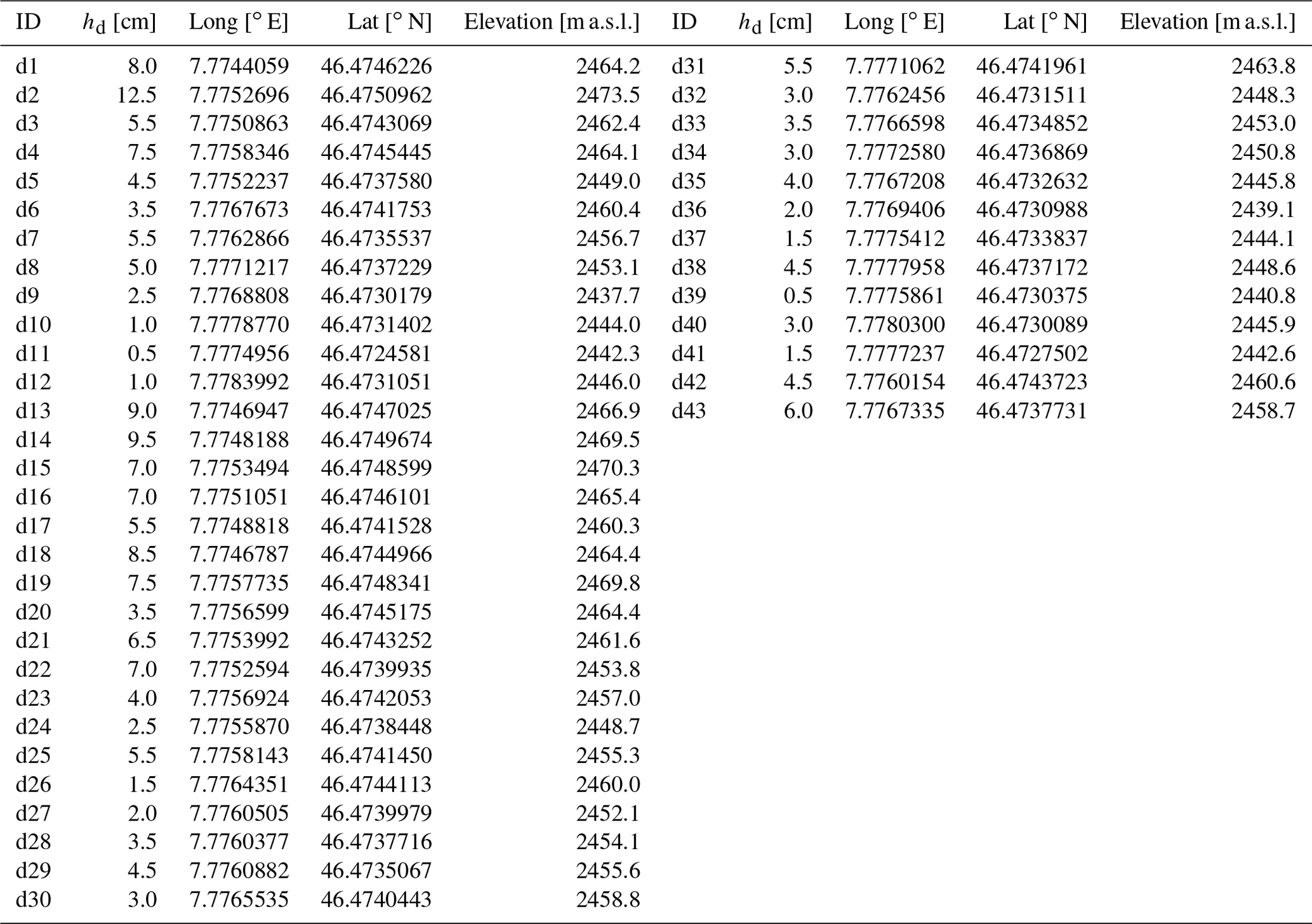
Table A2Mean debris temperature (at a depth of ca. 0.5–1.0 cm below the surface of the debris layer) during the two UAV surveys, measured with the tiny temperature loggers (see Fig. 1 and Sect. 3.3.2).
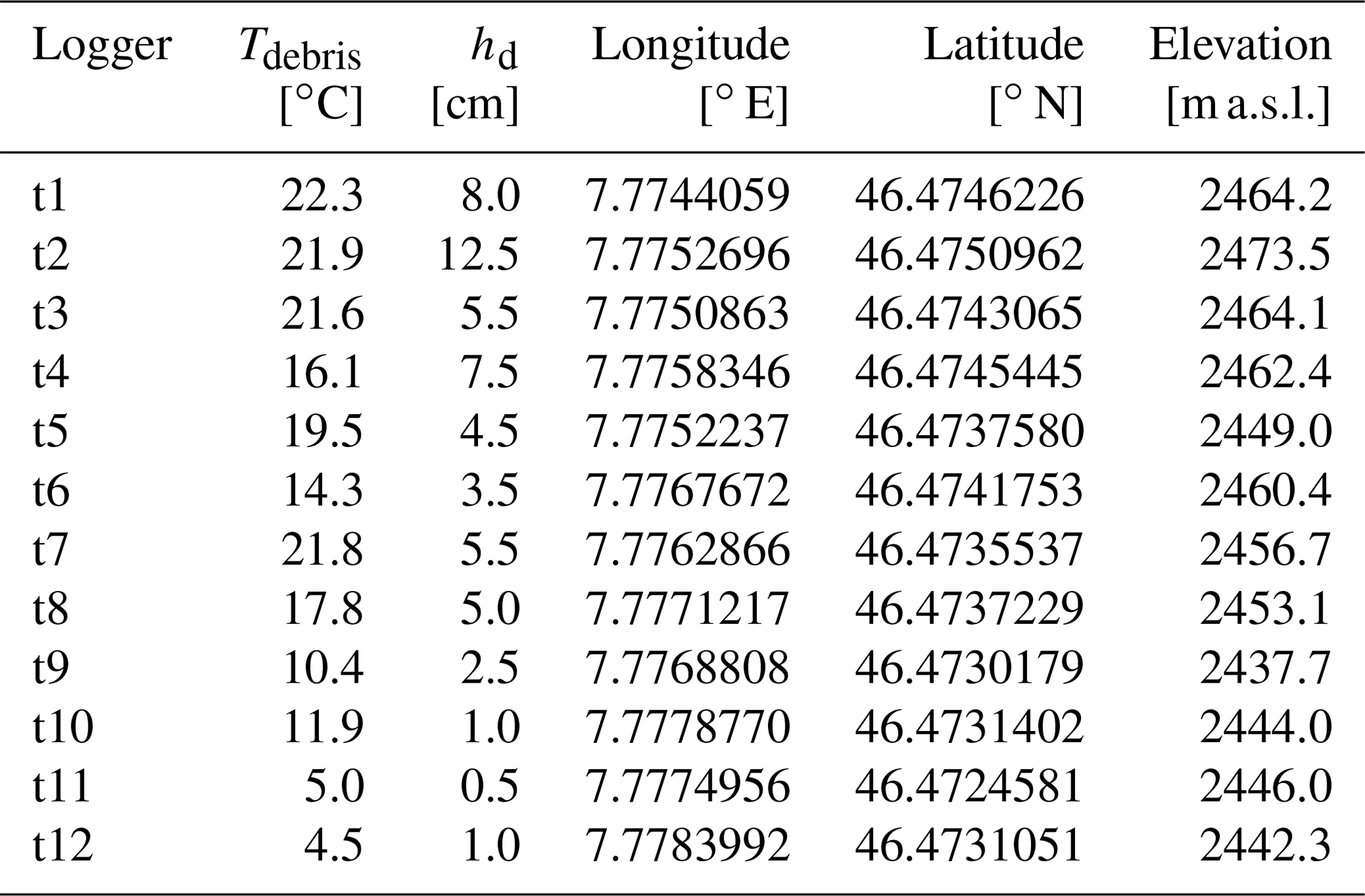
Table A3Positional accuracy of the visual orthophoto at each GCP measured with the differential GNSS device (see Fig. 1 and Sect. 3.2).
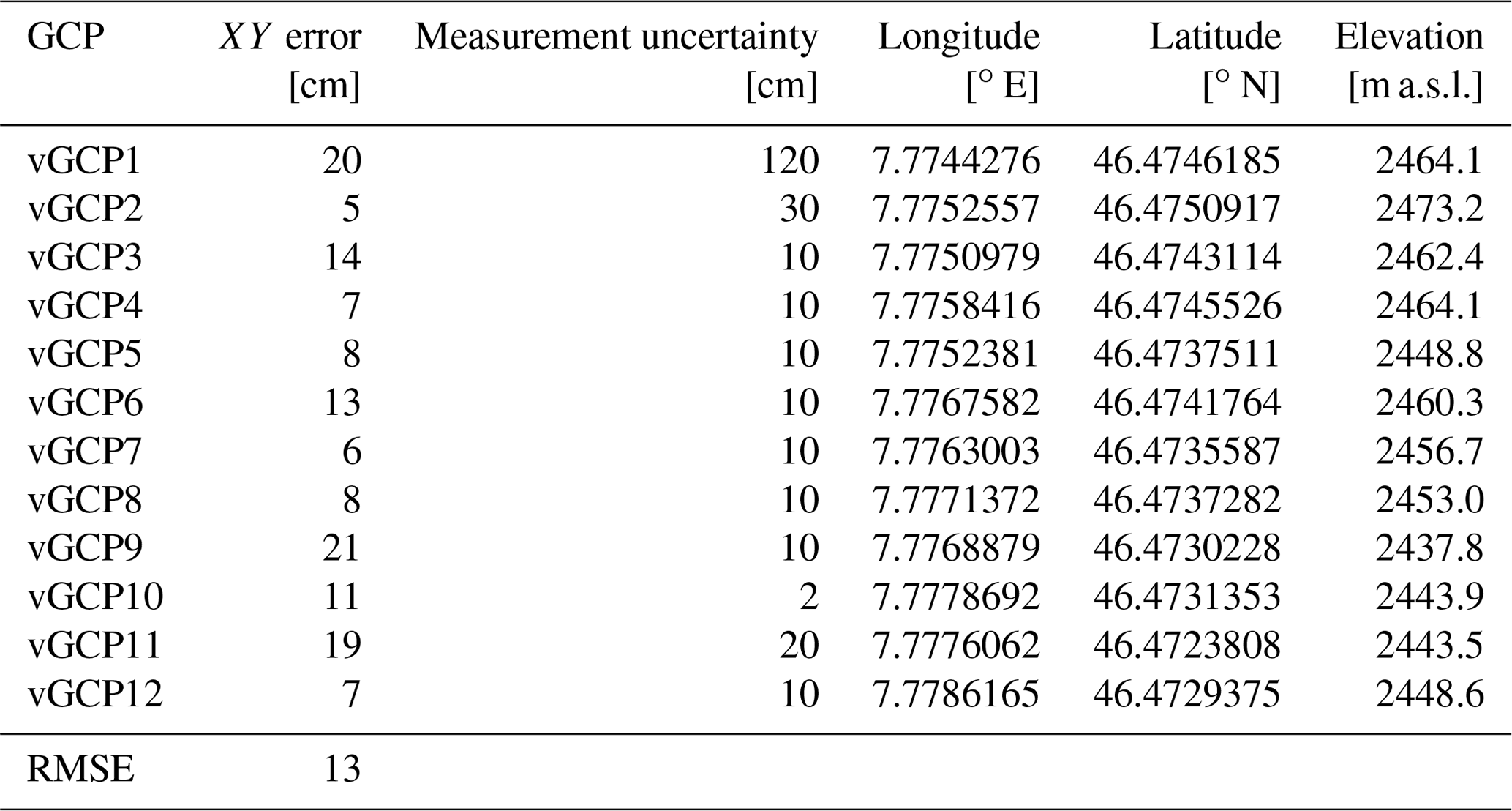
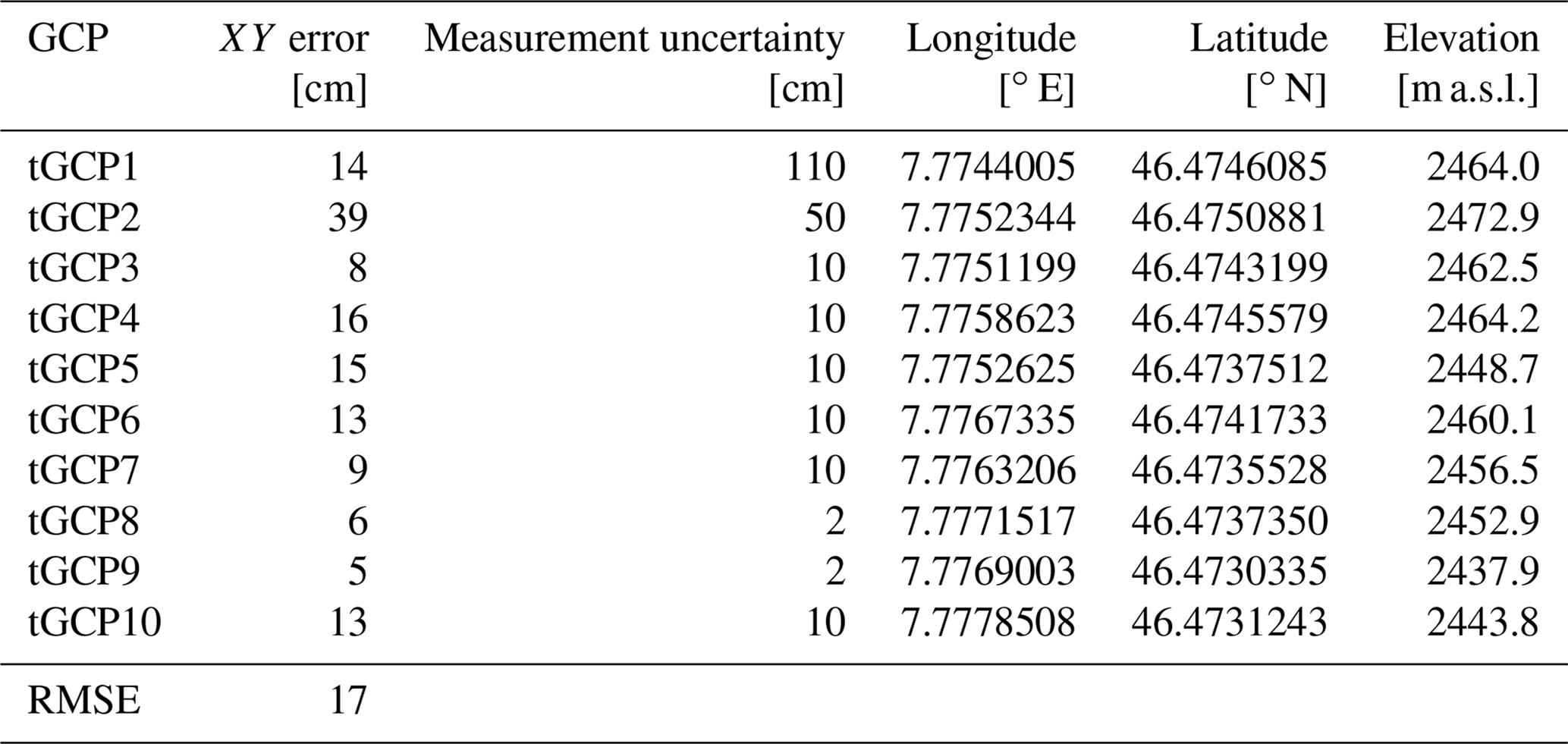
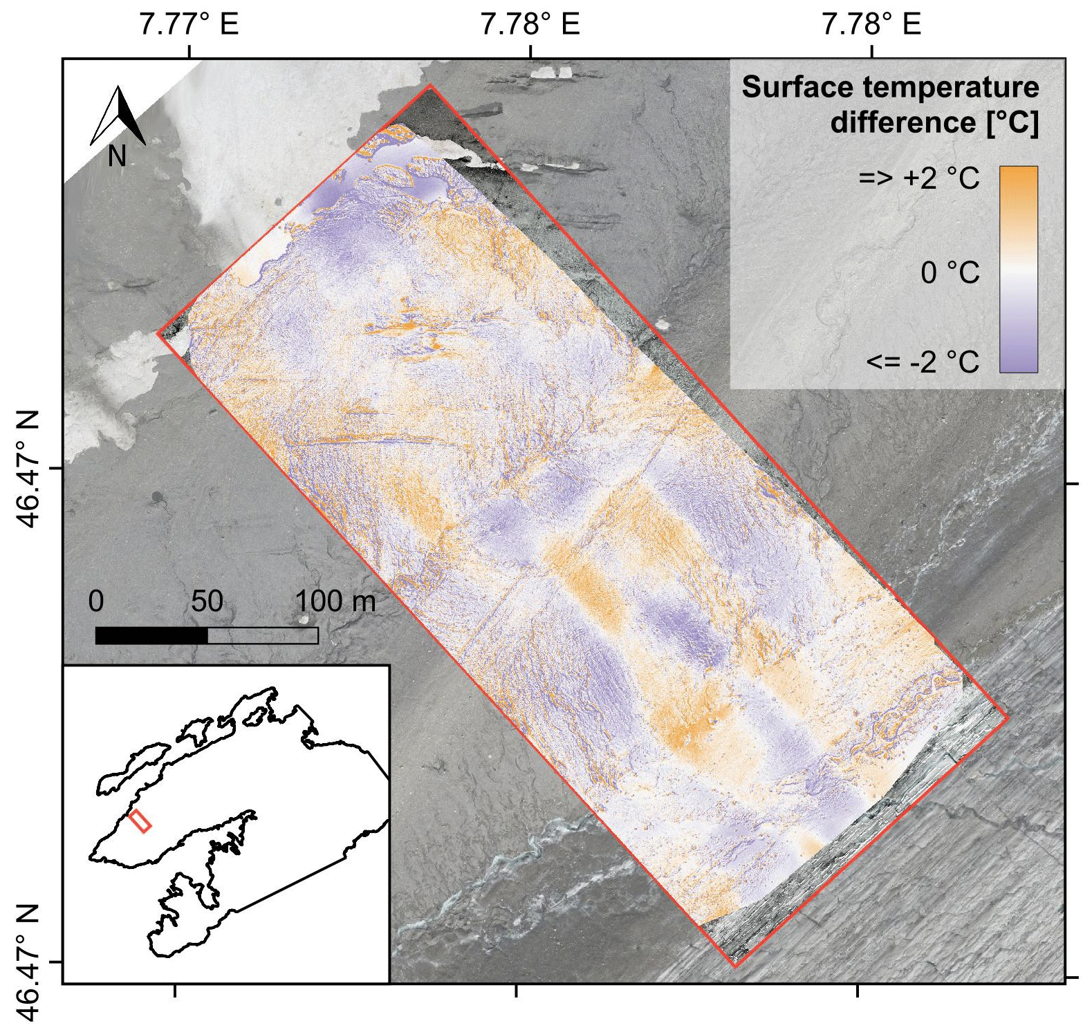
Figure B1Difference between the surface temperature map derived from the radiometric orthophoto generated with the open-source software ODM and the one derived from the radiometric orthophoto generated with the proprietary software Pix4Dmapper. Negative deviations indicate relatively higher surface temperatures in the ODM thermal orthophoto and vice versa.
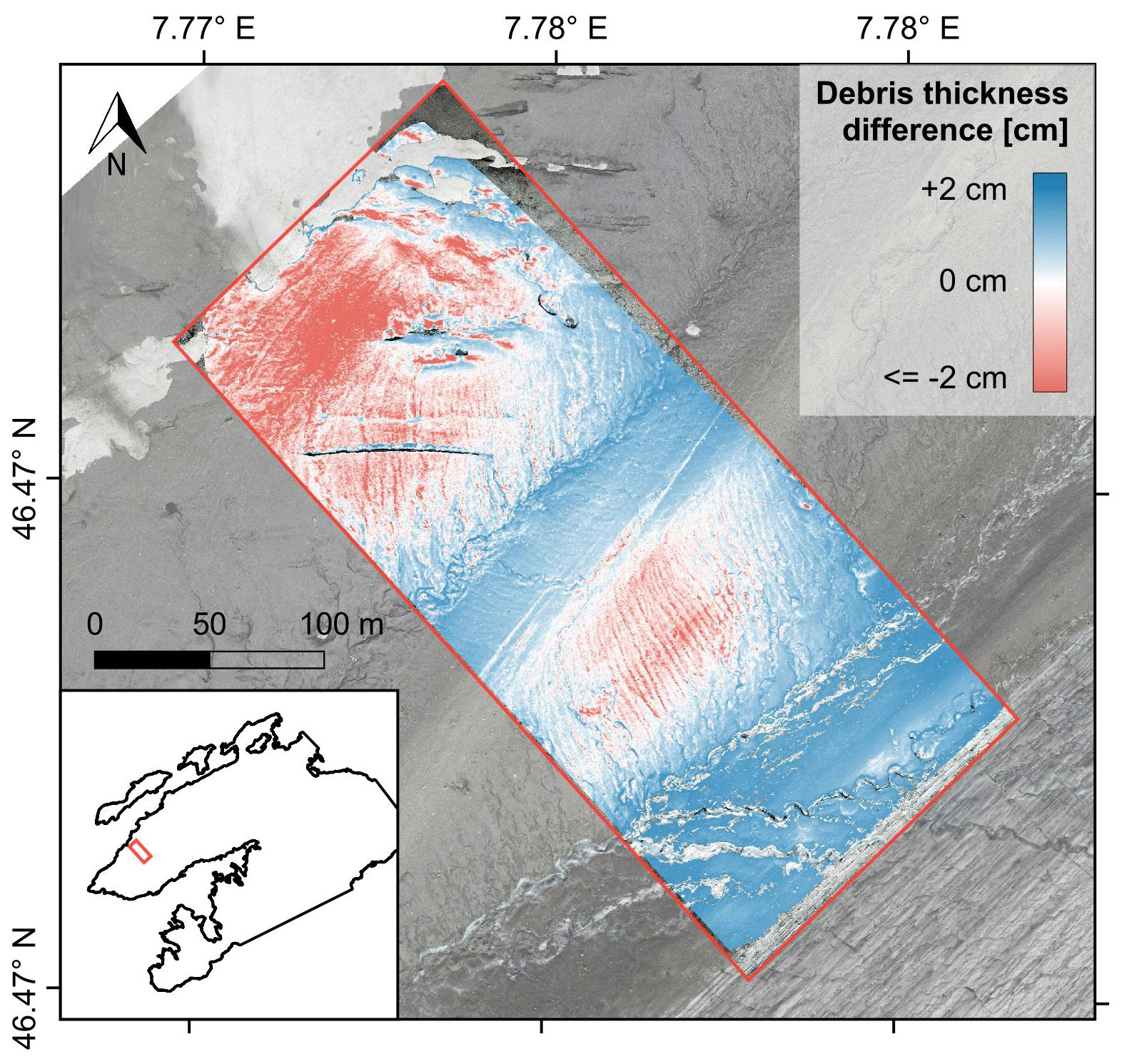
Figure C1Difference between the debris thickness map calculated with the empirical model (Eq. 9) and the one calculated with the inverse surface energy balance model (k=1.0 W m−1 K−1). Positive deviations (blue) indicate relatively higher debris thickness estimates in the empirical map and vice versa.
The complete dataset (including visual and thermal UAV images, in situ measurements, visual and radiometric orthophotos, and surface temperature and debris thickness maps), a QGIS project, and the open-source pipeline for data processing and debris thickness modelling can be downloaded via the open-access repository Zenodo: https://doi.org/10.5281/zenodo.10008937 (Messmer and Groos, 2023).
ARG designed the study, developed the customised mounting of the TIR camera on the quadcopter and implemented the surface energy balance model. JM carried out the fieldwork, performed the UAV surveys and processed most of the data. Both authors contributed equally to the development of the open-source pipeline, writing of the manuscript and generation of the figures.
The contact author has declared that neither of the authors has any competing interests.
Publisher's note: Copernicus Publications remains neutral with regard to jurisdictional claims made in the text, published maps, institutional affiliations, or any other geographical representation in this paper. While Copernicus Publications makes every effort to include appropriate place names, the final responsibility lies with the authors.
The expenses for the UAV surveys and field work on the Kanderfirn were covered by the Institute of Geography of the University of Bern. We thank Peter Leiser for helping with the customised mounting of the TIR camera on the quadcopter, Christoph Mayer for contributing to the implementation of the theoretical sub-debris ice melt model and Heinz Veit for the overall support of the study. We also very much appreciate the support of Rebecca Siebeneicher, Shayna Lindemann and Nicolas Brand during field work. The Swiss Federal Office of Meteorology and Climatology (MeteoSwiss) and the WSL Institute for Snow and Avalanche Research (SLF) kindly provided the meteorological data from Gandegg, Grächen, Fisistock and Jungfraujoch. We thank the editor Kang Yang and the two reviewers (Sam Herreid and one anonymous referee) for their constructive remarks during review, which greatly enhanced the structure and quality of the paper.
Open access funding was provided by the University of Bern and swissuniversities.
This paper was edited by Kang Yang and reviewed by Sam Herreid and one anonymous referee.
Anderson, L. S., Armstrong, W. H., Anderson, R. S., and Buri, P.: Debris cover and the thinning of Kennicott Glacier, Alaska: in situ measurements, automated ice cliff delineation and distributed melt estimates, The Cryosphere, 15, 265–282, https://doi.org/10.5194/tc-15-265-2021, 2021. a
Anderson, R. S., Anderson, L. S., Armstrong, W. H., Rossi, M. W., and Crump, S. E.: Glaciation of alpine valleys: The glacier – debris-covered glacier – rock glacier continuum, Geomorphology, 311, 127–142, https://doi.org/10.1016/j.geomorph.2018.03.015, 2018. a, b
Aubry-Wake, C., Baraër, M., McKenzie, J. M., Mark, B. G., Wigmore, O., Hellström, R. Å., Lautz, L., and Somers, L.: Measuring Glacier Surface Temperatures with Ground-Based Thermal Infrared Imaging, Geophys. Res. Lett., 42, 8489–8497, https://doi.org/10.1002/2015GL065321, 2015. a, b
Aubry-Wake, C., Zéphir, D., Baraër, M., McKenzie, J. M., and Mark, B. G.: Importance of Longwave Emissions from Adjacent Terrain on Patterns of Tropical Glacier Melt and Recession, J. Glaciol., 64, 49–60, https://doi.org/10.1017/jog.2017.85, 2018. a, b
Aubry-Wake, C., Lamontagne-Hallé, P., Baraër, M., McKenzie, J. M., and Pomeroy, J. W.: Using ground-based thermal imagery to estimate debris thickness over glacial ice: fieldwork considerations to improve the effectiveness, J. Glaciol., 69, 353–369, https://doi.org/10.1017/jog.2022.67, 2023. a, b, c, d, e
Avdelidis, N. P. and Moropoulou, A.: Emissivity considerations in building thermography, Energy Build., 35, 663–667, https://doi.org/10.1016/S0378-7788(02)00210-4, 2003. a
Baker, E. A., Lautz, L. K., McKenzie, J. M., and Aubry-Wake, C.: Improving the accuracy of time-lapse thermal infrared imaging for hydrologic applications, J. Hydrol., 571, 60–70, https://doi.org/10.1016/j.jhydrol.2019.01.053, 2019. a
Becker, F. and Li, Z.: Surface temperature and emissivity at various scales: Definition, measurement and related problems, Remote Sens. Rev., 12, 225–253, https://doi.org/10.1080/02757259509532286, 1995. a
Bisset, R. R., Nienow, P. W., Goldberg, D. N., Wigmore, O., Loayza-Muro, R. A., Wadham, J. L., Macdonald, M. L., and Bingham, R. G.: Using Thermal UAV Imagery to Model Distributed Debris Thicknesses and Sub-Debris Melt Rates on Debris-Covered Glaciers, J. Glaciol., 69, 981–996, https://doi.org/10.1017/jog.2022.116, 2022. a, b, c, d, e, f, g, h, i, j, k, l, m, n, o, p, q, r, s, t
Brun, F., Wagnon, P., Berthier, E., Shea, J. M., Immerzeel, W. W., Kraaijenbrink, P. D. A., Vincent, C., Reverchon, C., Shrestha, D., and Arnaud, Y.: Ice cliff contribution to the tongue-wide ablation of Changri Nup Glacier, Nepal, central Himalaya, The Cryosphere, 12, 3439–3457, https://doi.org/10.5194/tc-12-3439-2018, 2018. a
Buri, P., Miles, E. S., Steiner, J. F., Ragettli, S., and Pellicciotti, F.: Supraglacial Ice Cliffs Can Substantially Increase the Mass Loss of Debris-Covered Glaciers, Geophys. Res. Lett., 48, e2020GL092150, https://doi.org/10.1029/2020GL092150, 2021. a
Burton-Johnson, A. and Wyniawskyj, N. S.: Rock and snow differentiation from colour (RGB) images, The Cryosphere Discuss. [preprint], https://doi.org/10.5194/tc-2020-115, 2020. a
Cronholm, M.: Don’t let the RAT bite you!, InfraMation 2002 Conference, http://www.cronholm.com/files/32-Cronholm-2002.pdf (last access: 11 November 2021), 2002. a, b
Delaney, I. and Anderson, L. S.: Debris Cover Limits Subglacial Erosion and Promotes Till Accumulation, Geophys. Res. Lett., 49, e2022GL099049, https://doi.org/10.1029/2022GL099049, 2022. a
DJI: Mavic Pro Quick Start Guide V1.2, https://dl.djicdn.com/downloads/mavic/20170117/Mavic+Pro+Quick+Start+Guide+V1.2.pdf (last access: 4 November 2021), 2016. a
Evatt, G., Abrahams, I., Heil, M., Mayer, C., Kingslake, J., Michell, S., Fowler, A., and Clark, C.: Glacial melt under a porous debris layer, J. Glaciol., 61, 825–836, https://doi.org/10.3189/2015JoG14J235, 2015. a, b, c, d, e
Ferguson, J. C. and Vieli, A.: Modelling steady states and the transient response of debris-covered glaciers, The Cryosphere, 15, 3377–3399, https://doi.org/10.5194/tc-15-3377-2021, 2021. a, b
Fischer, M., Huss, M., Barboux, C., and Hoelzle, M.: The new Swiss Glacier Inventory SGI2010: relevance of using high-resolution source data in areas dominated by very small glaciers, Arct. Antarct. Alp. Res., 46, 933–945, https://doi.org/10.1657/1938-4246-46.4.933, 2014. a
FLIR Systems: FLIR Tools, https://www.flir.com/products/flir-tools/ (last access: 15 October 2021), 2015. a, b
Foster, L. A., Brock, B. W., Cutler, M. E. J., and Diotri, F.: A physically based method for estimating supraglacial debris thickness from thermal band remote-sensing data, J. Glaciol., 58, 677–691, https://doi.org/10.3189/2012JoG11J194, 2012. a, b, c, d
Gardelle, J., Berthier, E., Arnaud, Y., and Kääb, A.: Region-wide glacier mass balances over the Pamir-Karakoram-Himalaya during 1999–2011, The Cryosphere, 7, 1263–1286, https://doi.org/10.5194/tc-7-1263-2013, 2013. a
Gök, D. T., Scherler, D., and Anderson, L. S.: High-resolution debris-cover mapping using UAV-derived thermal imagery: limits and opportunities, The Cryosphere, 17, 1165–1184, https://doi.org/10.5194/tc-17-1165-2023, 2023. a, b, c, d, e, f, g, h, i, j, k, l, m, n, o, p, q
Groos, A., Mayer, C., Smiraglia, C., Diolaiuti, G., and Lambrecht, A.: A first attempt to model region-wide glacier surface mass balances in the Karakoram: Findings and future challenges, Geogr. Fis. Din. Quat., 40, 137–159, https://doi.org/10.4461/GFDQ.2017.40.10, 2017. a, b, c, d, e, f, g
Groos, A. R. and Mayer, C.: Glacier Surface Mass Balance Model “glacierSMBM” [R package], https://cran.r-project.org/src/contrib/Archive/glacierSMBM/ (last access: 2 December 2021), 2017. a
Groos, A. R., Bertschinger, T. J., Kummer, C. M., Erlwein, S., Munz, L., and Philipp, A.: The potential of low-cost UAVs and open-source photogrammetry software for high-resolution monitoring of alpine glaciers: A case study from the Kanderfirn (Swiss Alps), Geosciences, 9, 1–21, https://doi.org/10.3390/geosciences9080356, 2019. a, b, c, d, e, f
Groos, A. R., Aeschbacher, R., Fischer, M., Kohler, N., Mayer, C., and Senn-Rist, A.: Accuracy of UAV Photogrammetry in Glacial and Periglacial Alpine Terrain: A Comparison With Airborne and Terrestrial Datasets, Front. Remote Sens., 3, 16, https://doi.org/10.3389/frsen.2022.871994, 2022a. a, b, c, d
Groos, A. R., Niederhauser, J., Lemma, B., Fekadu, M., Zech, W., Hänsel, F., Wraase, L., Akçar, N., and Veit, H.: An hourly ground temperature dataset for 16 high-elevation sites (3493–4377 m a.s.l.) in the Bale Mountains, Ethiopia (2017–2020), Earth Syst. Sci. Data, 14, 1043–1062, https://doi.org/10.5194/essd-14-1043-2022, 2022b. a
Hansche, I., Shahi, S., Abermann, J., and Schöner, W.: The vertical atmospheric structure of the partially glacierised Mittivakkat valley, southeast Greenland, J. Glaciol., 69, 1097–1108, https://doi.org/10.1017/jog.2022.120, 2023. a, b
Harvey, P.: Exiftool, https://exiftool.org/ (last access: 31 October 2021), 2021. a, b
Herreid, S.: What Can Thermal Imagery Tell Us About Glacier Melt Below Rock Debris?, Front. Earth Sci., 9, 681059, https://doi.org/10.3389/feart.2021.681059, 2021. a, b, c, d, e, f, g, h
Herreid, S. and Pellicciotti, F.: The state of rock debris covering Earth’s glaciers, Nat. Geosci., 13, 621–627, https://doi.org/10.1038/s41561-020-0615-0, 2020. a
Hügi, T.: Vergleichende petrologische und geochemische Untersuchungen an Graniten des Aarmassivs, Bern, Kümmerly & Frey, 1956. a
Jouvet, G., Weidmann, Y., Kneib, M., Detert, M., Seguinot, J., Sakakibara, D., and Sugiyama, S.: Short-lived ice speed-up and plume water flow captured by a VTOL UAV give insights into subglacial hydrological system of Bowdoin Glacier, Remote Sens. Environ., 217, 389–399, https://doi.org/10.1016/j.rse.2018.08.027, 2018. a
Juen, M., Mayer, C., Lambrecht, A., Han, H., and Liu, S.: Impact of varying debris cover thickness on ablation: a case study for Koxkar Glacier in the Tien Shan, The Cryosphere, 8, 377–386, https://doi.org/10.5194/tc-8-377-2014, 2014. a, b, c, d
Kääb, A., Berthier, E., Nuth, C., Gardelle, J., and Arnaud, Y.: Contrasting Patterns of Early Twenty-First-Century Glacier Mass Change in the Himalayas, Nature, 488, 495–498, https://doi.org/10.1038/nature11324, 2012. a
Kelly, J., Kljun, N., Olsson, P.-O., Mihai, L., Liljeblad, B., Weslien, P., Klemedtsson, L., and Eklundh, L.: Challenges and best practices for deriving temperature data from an uncalibrated UAV thermal infrared camera, Remote Sens., 11, 1–21, https://doi.org/10.3390/rs11050567, 2019. a
Khadka, A., Wagnon, P., Brun, F., Shrestha, D., Lejeune, Y., and Arnaud, Y.: Evaluation of ERA5-Land and HARv2 Reanalysis Data at High Elevation in the Upper Dudh Koshi Basin (Everest Region, Nepal), J. Appl. Meteorol. Climatol., 61, 931–954, https://doi.org/10.1175/JAMC-D-21-0091.1, 2022. a
Kraaijenbrink, P. D. A., Bierkens, M. F. P., Lutz, A. F., and Immerzeel, W. W.: Impact of a Global Temperature Rise of 1.5 Degrees Celsius on Asia's Glaciers, Nature, 549, 257–260, https://doi.org/10.1038/nature23878, 2017. a
Kraaijenbrink, P. D. A., Shea, J. M., Litt, M., Steiner, J. F., Treichler, D., Koch, I., and Immerzeel, W. W.: Mapping surface temperatures on a debris-covered glacier with an unmanned aerial vehicle, Front. Earth Sci., 6, 64, https://doi.org/10.3389/feart.2018.00064, 2018. a, b, c, d, e, f, g, h, i, j, k, l, m, n, o, p, q
Maisch, M., Wipf, A., Denneler, B., Battaglia, J., and Benz, C.: Die Gletscher der Schweizer Alpen: Gletscherhochstand 1850, Aktuelle Vergletscherung, Gletscherschwund-Szenarien, Tech. rep., Zürich: vdf Hochschulverlag, ISBN 9783728125682, 3728125687, 2000. a
Mayer, C. and Licciulli, C.: The Concept of Steady State, Cyclicity and Debris Unloading of Debris-Covered Glaciers, Front. Earth Sci., 9, https://doi.org/10.3389/feart.2021.710276, 2021. a, b
McCarthy, M., Pritchard, H., Willis, I., and King, E.: Ground-penetrating radar measurements of debris thickness on Lirung Glacier, Nepal, J. Glaciol., 63, 543–555, https://doi.org/10.1017/jog.2017.18, 2017. a
McCarthy, M., Miles, E., Kneib, M., Buri, P., Fugger, S., and Pellicciotti, F.: Supraglacial Debris Thickness and Supply Rate in High-Mountain Asia, Commun. Earth Environ., 3, 269, https://doi.org/10.1038/s43247-022-00588-2, 2022. a, b
Messmer, J. and Groos, A. R.: A low-cost and open-source approach for supraglacial debris thickness mapping using UAV-based infrared thermography (v2.0.0), Zenodo [data set], https://doi.org/10.5281/zenodo.10008937, 2023. a
Mihalcea, C., Mayer, C., Diolaiuti, G., Lambrecht, A., Smiraglia, C., and Tartari, G.: Ice Ablation and Meteorological Conditions on the Debris-Covered Area of Baltoro Glacier, Karakoram, Pakistan, Ann. Glaciol., 43, 292–300, https://doi.org/10.3189/172756406781812104, 2006. a
Mihalcea, C., Brock, B. W., Diolaiuti, G., D'Agata, C., Citterio, M., Kirkbride, M. P., Cutler, M. E. J., and Smiraglia, C.: Using ASTER satellite and ground-based surface temperature measurements to derive supraglacial debris cover and thickness patterns on Miage Glacier (Mont Blanc Massif, Italy), Cold Reg. Sci. Technol., 52, 341–354, https://doi.org/10.1016/j.coldregions.2007.03.004, 2008a. a, b, c, d
Mihalcea, C., Mayer, C., Diolaiuti, G., D’Agata, C., Smiraglia, C., Lambrecht, A., Vuillermoz, E., and Tartari, G.: Spatial distribution of debris thickness and melting from remote-sensing and meteorological data, at debris-covered Baltoro glacier, Karakoram, Pakistan, Ann. Glaciol., 48, 49–57, https://doi.org/10.3189/172756408784700680, 2008b. a, b, c, d, e
Miles, E. S., Willis, I., Buri, P., Steiner, J. F., Arnold, N. S., and Pellicciotti, F.: Surface Pond Energy Absorption Across Four Himalayan Glaciers Accounts for 1/8 of Total Catchment Ice Loss, Geophys. Res. Lett., 45, 10464–10473, https://doi.org/10.1029/2018GL079678, 2018. a
Mineo, S. and Pappalardo, G.: Rock emissivity measurement for infrared thermography engineering geological applications, Appl. Sci., 11, 3773, https://doi.org/10.3390/app11093773, 2021. a, b, c, d
Minkina, W. and Dudzik, S.: Algorithm of Infrared Camera Measurement Processing Path, in: Infrared Thermography: Errors and Uncertainties, Chichester, John Wiley & Sons, Ltd, Chichester UK, 60–81, 2009. a, b, c, d, e
Minnis, P. and Khaiyer, M.: Anisotropy of land surface skin temperature derived from satellite data, J. Appl. Meteorol., 39, 1117–1129, https://doi.org/10.1175/1520-0450(2000)039<1117:AOLSST>2.0.CO;2, 2000. a
Naegeli, K., Huss, M., and Hoelzle, M.: Change detection of bare-ice albedo in the Swiss Alps , The Cryosphere, 13, 397–412, https://doi.org/10.5194/tc-13-397-2019, 2019. a
National Physical Laboratory: What is emissivity and why is it important?, https://www.npl.co.uk/resources/q-a/why-is-emissivity-important (last access: 22 November 2021), 2021. a, b
Nicholson, L. and Benn, D. I.: Calculating Ice Melt beneath a Debris Layer Using Meteorological Data, J. Glaciol., 52, 463–470, https://doi.org/10.3189/172756506781828584, 2006. a, b, c
Nicholson, L. and Benn, D. I.: Properties of natural supraglacial debris in relation to modelling sub-debris ice ablation, Earth Surf. Process. Land., 38, 490–501, https://doi.org/10.1002/esp.3299, 2013. a
Nicholson, L. and Mertes, J.: Thickness estimation of supraglacial debris above ice cliff exposures using a high-resolution digital surface model derived from terrestrial photography, J. Glaciol., 63, 989–998, https://doi.org/10.1017/jog.2017.68, 2017. a
Paul, F.: The new Swiss glacier inventory 2000 – application of remote sensing and GIS, PhD Thesis, University of Zurich, Zurich, https://doi.org/10.5167/uzh-163148, 2003. a
Pix4D: Pix4Dmapper, https://www.pix4d.com/de/produkt/pix4dmapper-photogrammetrie-software (last access: 8 November 2021), 2021a. a
Pix4D: Reflectance map vs orthomosaic, https://support.pix4d.com/hc/en-us/articles/202739409-Reflectance-map-vs-orthomosaic (last Access: 11 November 2021), 2021b. a
Pour, T., Miřijovský, J., and Purket, T.: Airborne thermal remote sensing: the case of the city of Olomouc, Czech Republic, Eur. J. Remote Sens., 52, 209–218, https://doi.org/10.1080/22797254.2018.1564888, 2019. a, b, c, d
QGIS Development Team: QGIS Desktop, http://qgis.osgeo.org (last access: 5 November 2021), 2020. a
R Core Team: R: A language and environment for statistical computing, https://cran.r-project.org/bin/windows/base/ (last access: 5 November 2021), 2019. a
Ribeiro-Gomes, K., Hernández-López, D., Ortega, J. F., Ballesteros, R., Poblete, T., and Moreno, M. A.: Uncooled Thermal Camera Calibration and Optimization of the Photogrammetry Process for UAV Applications in Agriculture, Sensors, 17, 2173, https://doi.org/10.3390/s17102173, 2017. a, b
Rivard, B., Thomas, P. J., and Giroux, J.: Precise emissivity of rock samples, Remote Sens. Environ., 54, 152–160, https://doi.org/10.1016/0034-4257(95)00130-S, 1995. a, b, c, d
Rounce, D. R. and McKinney, D. C.: Debris thickness of glaciers in the Everest area (Nepal Himalaya) derived from satellite imagery using a nonlinear energy balance model, The Cryosphere, 8, 1317–1329, https://doi.org/10.5194/tc-8-1317-2014, 2014. a, b, c, d, e
Rounce, D. R., King, O., McCarthy, M., Shean, D. E., and Salerno, F.: Quantifying debris thickness of debris-covered glaciers in the Everest region of Nepal through inversion of a subdebris melt model, J. Geophys. Res.-Earth, 123, 1094–1115, https://doi.org/10.1029/2017JF004395, 2018. a, b, c
Rounce, D. R., Hock, R., and Shean, D. E.: Glacier Mass Change in High Mountain Asia Through 2100 Using the Open-Source Python Glacier Evolution Model (PyGEM), Front. Earth Sci., 7, 331, https://doi.org/10.3389/feart.2019.00331, 2020. a
Rounce, D. R., Hock, R., McNabb, R. W., Millan, R., Sommer, C., Braun, M. H., Malz, P., Maussion, F., Mouginot, J., Seehaus, T. C., and Shean, D. E.: Distributed global debris thickness estimates reveal debris significantly impacts glacier mass balance, Geophys. Res. Lett., 48, 1–12, https://doi.org/10.1029/2020GL091311, 2021. a, b, c, d, e, f, g, h, i
Rowan, A. V., Egholm, D. L., Quincey, D. J., and Glasser, N. F.: Modelling the Feedbacks between Mass Balance, Ice Flow and Debris Transport to Predict the Response to Climate Change of Debris-Covered Glaciers in the Himalaya, Earth Planet. Sc. Lett., 430, 427–438, https://doi.org/10.1016/j.epsl.2015.09.004, 2015. a
Ryan, J. C., Hubbard, A., Box, J. E., Brough, S., Cameron, K., Cook, J. M., Cooper, M., Doyle, S. H., Edwards, A., Holt, T., Irvine-Fynn, T., Jones, C., Pitcher, L. H., Rennermalm, A. K., Smith, L. C., Stibal, M., and Snooke, N.: Derivation of High Spatial Resolution Albedo from UAV Digital Imagery: Application over the Greenland Ice Sheet, Front. Earth Sci., 5, 40, https://doi.org/10.3389/feart.2017.00040, 2017. a
Sagan, V., Maimaitijiang, M., Sidike, P., Eblimit, K., Peterson, K., Hartling, S., Esposito, F., Khanal, K., Newcomb, M., Pauli, D., Ward, R., Fritschi, F., Shakoor, N., and Mockler, T.: UAV-Based High Resolution Thermal Imaging for Vegetation Monitoring, and Plant Phenotyping Using ICI 8640 P, FLIR Vue Pro R 640, and thermoMap Cameras, Remote Sens., 11, 1–29, https://doi.org/10.3390/rs11030330, 2019. a
Sakai, A., Nakawo, M., and Fujita, K.: Melt rate of ice cliffs on the Lirung Glacier, Nepal Himalayas, 1996, B. Glacier Res., 16, 57–66, 1998. a
Salisbury, J. W. and D'Aria, D. M.: Emissivity of terrestrial materials in the 8–14 μm atmospheric window, Remote Sens. Environ., 42, 83–106, https://doi.org/10.1016/0034-4257(92)90092-X, 1992. a, b, c
Schauwecker, S., Rohrer, M., Huggel, C., Kulkarni, A., Ramanathan, A., Salzmann, N., Stoffel, M., and Brock, B.: Remotely sensed debris thickness mapping of Bara Shigri Glacier, Indian Himalaya, J. Glaciol., 61, 675–688, https://doi.org/10.3189/2015JoG14J102, 2015. a
Scherler, D., Bookhagen, B., and Strecker, M. R.: Spatially Variable Response of Himalayan Glaciers to Climate Change Affected by Debris Cover, Nat. Geosci., 4, 156–159, https://doi.org/10.1038/NGEO1068, 2011. a
Scherler, D., Wulf, H., and Gorelick, N.: Global assessment of supraglacial debris-cover extents, Geophys. Res. Lett., 45, 11798–11805, https://doi.org/10.1029/2018GL080158, 2018. a
Steiner, J. F., Pellicciotti, F., Buri, P., Miles, E. S., Immerzeel, W. W., and Reid, T. D.: Modelling Ice-Cliff Backwasting on a Debris-Covered Glacier in the Nepalese Himalaya, J. Glaciol., 61, 889–907, https://doi.org/10.3189/2015JoG14J194, 2015. a
Steiner, J. F., Kraaijenbrink, P. D. A., and Immerzeel, W. W.: Distributed Melt on a Debris-Covered Glacier: Field Observations and Melt Modeling on the Lirung Glacier in the Himalaya, Front. Earth Sci., 9, 678375, https://doi.org/10.3389/feart.2021.678375, 2021. a, b, c
Swiss Federal Office of Topography: SWISSIMAGE [WMS], https://www.swisstopo.admin.ch/en/orthoimage-swissimage-10 (last access: 12 February 2024), 2021. a, b
Swiss Federal Office of Topography, Geological Institute, University of Bern, and Federal Office for Water und Geology: Geological Map of Switzerland 1:500 000, Swiss Federal Office of Topography, Wabern, https://opendata.swiss/en/perma/ca917a71-dcc9-44b6-8804-823c694be516@bundesamt-fur-landestopografie-swisstopo (last access: 12 February 2024), 2005. a
Tarca, G. and Guglielmin, M.: Using Ground-Based Thermography to Analyse Surface Temperature Distribution and Estimate Debris Thickness on Gran Zebrù Glacier (Ortles-Cevedale, Italy), Cold Reg. Sci. Technol., 196, 103487, https://doi.org/10.1016/j.coldregions.2022.103487, 2022. a, b
Tattersall: Thermimage: Thermal Image Analysis, raw2temp source code, https://github.com/gtatters/Thermimage/blob/7bd5a9afcd4164cfa58a8e2c5fd9fac2ca1f40ab/R/raw2temp.R (last access: 8 October 2021), 2019. a, b
Tattersall: Thermimage: Thermal Image Analysis [R package], https://cran.r-project.org/web/packages/Thermimage (last access: 8 October 2021), 2021a. a, b, c, d, e, f, g
Tattersall: Thermimage: Thermal Image Analysis Reference manual, https://cran.r-project.org/web/packages/Thermimage/Thermimage.pdf (last access: 8 October 2021), 2021b. a, b
Teledyne FLIR: sUAS Radiometry Technical Note, https://dl.djicdn.com/downloads/zenmuse_xt/en/sUAS_Radiometry_Technical_Note.pdf (last access: 9 December 2021), 2016. a
Teledyne FLIR: Time Constant Design of Tau2 and Quark2, https://flir.custhelp.com/app/answers/detail/a_id/3171/~/time-constant-design-of-tau2-and-quark2/session/ (last access: 9 December 2021), 2019a. a
Teledyne FLIR: FLIR Vue Pro R Datasheet, https://www.flir.eu/products/vue-pro-r/?vertical=suas&segment=oem (last access: 12 February 2024), 2019b. a
Teledyne FLIR: How Does Emissivity Affect Thermal Imaging?, https://www.flir.com/discover/professional-tools/how-does-emissivity-affect-thermal-imaging/ (last access: 11 January 2022), 2021a. a
Teledyne FLIR: Thermal Studio Suite, https://www.flir.com/products/flir-thermal-studio-suite/ (last access: 12 August 2021), 2021b. a, b
Tempmate: tempmate.®-B series ultra robust miniature data loggers, https://www.tempmate.com/temperature-logger/tempmate-b-series/ (last access: 17 February 2022), 2022. a
USGS UAS: Workflow for Generating Orthomosaics from FLIR Vue PRO R 13mm Imagery in Agisoft PhotoScan/Metashape, https://uas.nifc.gov/sites/default/files/sites/default/files/inline-files/UASD_FLIR Vue PRO R Workflow_USGS_2019.07.28.pdf (last access: 4 November 2021), 2019. a
van Dongen, E. C. H., Jouvet, G., Sugiyama, S., Podolskiy, E. A., Funk, M., Benn, D. I., Lindner, F., Bauder, A., Seguinot, J., Leinss, S., and Walter, F.: Thinning leads to calving-style changes at Bowdoin Glacier, Greenland, The Cryosphere, 15, 485–500, https://doi.org/10.5194/tc-15-485-2021, 2021. a
van Woerkom, T., Steiner, J. F., Kraaijenbrink, P. D. A., Miles, E. S., and Immerzeel, W. W.: Sediment supply from lateral moraines to a debris-covered glacier in the Himalaya, Earth Surf. Dynam., 7, 411–427, https://doi.org/10.5194/esurf-7-411-2019, 2019. a
VC Technology: Litchi, https://flylitchi.com/ (last access: 23 June 2021), 2020. a
VC Technology: Litchi Mission Hub, https://flylitchi.com/hub (last access: 27 September 2021), 2021. a
Virtue, J., Turner, D., Williams, G., Zeliadt, S., McCabe, M., and Lucieer, A.: Thermal Sensor Calibration for Unmanned Aerial Systems Using an External Heated Shutter, Drones, 5, 119, https://doi.org/10.3390/drones5040119, 2021. a, b, c
Wirbel, A., Jarosch, A. H., and Nicholson, L.: Modelling debris transport within glaciers by advection in a full-Stokes ice flow model, The Cryosphere, 12, 189–204, https://doi.org/10.5194/tc-12-189-2018, 2018. a
Østrem, G.: Ice melting under a thin layer of moraine, and the existence of ice cores in moraine ridges, Geogr. Ann., 41, 228–230, https://doi.org/10.1080/20014422.1959.11907953, 1959. a, b, c
- Abstract
- Introduction
- Study site
- Data and methods
- Results
- Discussion
- Conclusions
- Appendix A: In situ measurements
- Appendix B: Thermal orthophoto comparison
- Appendix C: Debris thickness map comparison
- Code and data availability
- Author contributions
- Competing interests
- Disclaimer
- Acknowledgements
- Financial support
- Review statement
- References