Extreme events of snow grain size increase in East Antarctica and their relationship with meteorological conditions

This study explores the seasonal variations in snow grain size on the East Antarctic Plateau, where dry metamorphism occurs, by using microwave radiometer observations from 2000 to 2022. Local meteorological conditions and large-scale atmospheric phenomena have been considered in order to explain some peculiar changes in the snow grains. We find that the highest ice divide is the region with the largest grain size in the summer, mainly because the wind speed is low. Moreover, some extreme grain size values with respect to the average (over +3σ) were identified. In these cases, the ERA5 reanalysis revealed a high-pressure blocking close to the onsets of the summer increase in the grain size. It channels moisture intrusions from the mid-latitudes, through atmospheric rivers that cause major snowfall events over the plateau. If conditions of weak wind and low temperature occur during the following weeks, dry snow metamorphism is facilitated, leading to grain growth. This determines anomalous high maximums of the snow grain size at the end of summer. These phenomena confirm the importance of moisture intrusion events in East Antarctica and their impact on the physical properties of the ice sheet surface, with a co-occurrence of atmospheric rivers and seasonal changes in the grain size with a significance of over 95 %.

1 Introduction

Understanding and modelling the physical changes in snow properties, in particular the grain size, is important to predict the changes in snowpack albedo (Grenfell et al., 1994; Domine et al., 2006) and hence in the surface energy balance at high latitudes. Moreover, it provides information on the firn properties, useful to retrieve the ice sheet mass balance by spaceborne altimetry (Keenan et al., 2021; Kingslake et al., 2022). The seasonal variations in the grain size observed by spaceborne microwave radiometer in Antarctica show a large summer increase, which is mainly driven by temperature (Picard et al., 2012). The increase in temperature during austral summer leads to coarsening of snow grains due to grain-to-grain transport of water vapour (Colbeck, 1982, 1993; Sturm and Benson, 1997; Flanner and Zender, 2006; Town et al., 2008), while winter precipitations and wind-transported snow accumulate small grains over the surface (Domine et al., 2007). On the East Antarctic Plateau the mean annual precipitation is low, less than 100 kg m⁻² in the highest part of the ice sheet, due to its isolation from the rest of the hemisphere (Palerme et al., 2014). However, some relatively warm and moist oceanic air masses occasionally travel far inland, providing higher-than-usual snow accumulations (Turner et al., 2019). These intrusions could be linked to atmospheric rivers known to transport warm and moist air from subtropics or mid-latitudes to the polar latitudes (e.g. Wille et al., 2021).

On the Antarctic Plateau, in situ observations of snow structure are rare and the meteorological measurements, needed to interpret the causes of changes in the snowpack, are sparse. This is the reason for the constant need of supplementary data coming, for example, from satellite observations, able to provide continuous information on snow surface characteristics at continental scale. Previous studies investigated the snow grain size retrieved from remote sensing observations. In Jin et al. (2008) near-infrared and visible satellite observations were exploited to retrieve the grain size in the top 1 cm during clear-sky conditions and observed widespread summer increase in the grain size. Picard et al. (2012) combined high-frequency passive microwave observations to implement an indicator of grain size in the uppermost ∼10 cm of the snowpack and compared it to observations at Dome C and simulation results obtained by modelling water vapour transport near the surface. They observed inter-annual variability in the summer grain growth and linked them to precipitation variability. Casado et al. (2021) also focused on Dome C, deepening the link between the water isotopic signature and surface snow metamorphism, observing changes in this grain size indicator for two contrasted summers (2014 and 2015). Hence, past studies were limited to clear-sky conditions or to a particular location (Dome C). Our work, by means of high-frequency microwave observations, explores the interaction between surface snow grain size and meteorological conditions, on a continental scale and on a seasonal time frame.

This work focuses on extremes of large grain sizes. The investigated events were recorded during summer between 2000 and 2022, close to the highest elevation points of the East Antarctica Plateau, along the ice divide. Using both passive microwave observations and atmospheric reanalysis, we investigate the physical processes involved in these events and their link with the local and regional atmospheric conditions.

The paper is organized as follows. Sections 2 and 3 present the satellite and meteorological datasets and statistical tools. Section 4 shows the results by firstly describing the common features of the grain size summer increases and their relationship with local meteorological conditions (Sect. 4.1), secondly focusing the analysis on the four most extreme grain size increases (Sect. 4.2), and lastly connecting the changes in the grain size with large-scale meteorological conditions (Sect. 4.3). In Sect. 5 we discuss the results, and Sect. 6 draws conclusions.

2 Materials

2.1 Passive microwave observations

We use the Advanced Microwave Sounding Unit-B (AMSU-B), which is a five-channel microwave radiometer operating since 1998 on board NOAA-15 to NOAA-19 and Metop (Meteorological Operational) satellites. Swath data from the sensors of NOAA-15 to NOAA-19 were downloaded from the National Centers for Environmental Information (https://www.avl.class.noaa.gov/, last access: February 2023) and, after selecting incidence angles in the range 0–25^∘, processed to obtain daily mean from January 2000 to May 2022 in southern polar stereographic projection (EPSG:3976) at a resolution of 25 km. Brightness temperatures observed at 89 and 150 GHz are then used to compute the snow grain size index (GSI) defined as $\mathrm{1}-T_{\mathrm{B}}\left(\mathrm{150}\mathrm{GHz}\right)/T_{\mathrm{B}}\left(\mathrm{89}\mathrm{GHz}\right)$ by Picard et al. (2012). They focused their study on Dome C and provided an approximate correspondence between the index and size in millimetres: 0.00 of GSI is ∼0.025 mm and 0.20 is ∼0.150 mm (for the grains in the first 7 cm of the snowpack). Because of the particular nature and high sensitivity of the microwaves to liquid water, GSI is only effective in regions where snowmelt never occurs, such as the East Antarctic Plateau (Picard et al., 2007).

2.2 Meteorological data

2.2.1 ERA5 reanalysis

For this study, we use skin temperature, 2 m temperature, 10 m wind speed, snowfall, surface pressure, cloud cover, and surface downward long-wave and short-wave radiation flux over Antarctica from the ERA5 reanalysis produced by the European Centre for Medium-Range Weather Forecasts (ECMWF; Hersbach et al., 2018a, b). Data are provided over a regular latitude–longitude grid of 0.25${}^{{}^{\circ }}$, and we reprojected them using the southern polar stereographic projection. We used not only daily means from 2000 to 2022 but also hourly values as inputs for the thermal model.

2.2.2 Atmospheric-river catalogues

The atmospheric-river (AR from now on) presence is obtained from the two catalogues built by Wille et al. (2021). The detection is based on the integrated water vapour (IWV) and the meridional component of the integrated vapour transport (vIVT), both from 3-hourly data of ERA5 and of the Modern-Era Retrospective analysis for Research and Applications, Version 2 (MERRA-2), reanalysis (Gelaro et al., 2017). The datasets provide a Boolean indicator of the AR presence for each grid cell worldwide with a latitude–longitude resolution of 0.50^∘ × 0.625^∘. Previous work revealed weak sensitivity to the input meteorological dataset used to study the climatology of ARs, between MERRA-2 (used for the tier-2 exercise of the ARTMIP project, Collow et al., 2022) and ERA5, especially over East Antarctica, even though important differences could arise when considering individual events (Pohl et al., 2021; Wille et al., 2021).

2.2.3 Antarctic Oscillation index

The Antarctic Oscillation index (AAO; also known as the Southern Annular Mode, SAM) (Thompson and Wallace, 2000) is provided by the National Oceanic and Atmospheric Administration (NOAA) and based on the daily anomalies of 700 hPa geopotential height south of 20^∘ S. In this study, we used the daily index over the 2000–2022 period (https://www.cpc.ncep.noaa.gov/products/precip/CWlink/daily_ao_index/aao/aao.shtml, last access: February 2023).

2.3 Snowpack temperature

The vertical profile of temperature in the upper snowpack is estimated with the surface energy budget and thermal diffusion model called the minimal firn model (MFM; https://github.com/ghislainp/mfm, last access: February 2023, Picard et al., 2009, 2012; Domine et al., 2019) inspired by the minimal snow model (Essery, 2004). The model takes as input 2 m air temperature, surface pressure, 10 m wind speed, 2 m specific humidity, surface downwelling long-wave radiation flux and surface downwelling short-wave radiation flux extracted from the hourly ERA5 reanalysis. Otherwise, the required snowpack properties are taken from the literature: the density at the surface and at 10 m depth (e.g. Leduc-Leballeur et al., 2015; Tian et al., 2018), the thermal conductivity (Boone, 2002), the specific heat capacity of ice (Picard et al., 2009) and the temperature at 10 m depth (equivalent to the mean annual air temperature in the Antarctic dry zones, Wang and Hou (2010)). From the MFM outputs, we used the temperature at 10 cm depth and the temperature gradient in the subsurface, defined as the difference between temperatures estimated at 0 and 1 cm in depth (positive gradient when the surface is colder than the subsurface).

3 Methods

To investigate the atmospheric processes which generate the highest snow grain size occurrences over the East Antarctic Plateau, we used the GSI defined by Picard et al. (2012) as a proxy for the snow grain size. We selected four case studies. In particular, we studied the GSI summer changes in order to compare the mean variations with the variation during which the highest GSI occurs and we analysed the large-scale atmospheric circulation during each case study.

3.1 Detection of the highest GSI over East Antarctica

We define an extreme grain size as GSI being higher than 0.23. This value is the 99.5th percentile of all the maximum GSI over the dry area in Antarctica in the period 2000–2022 and is significantly higher (p value = 0.012) than the mean annual maximum values of 0.11±0.01 typical of the East Antarctica ice divide. Figure 1 shows the maximum GSI over 2000–2022 derived from AMSU-B observations. Four extreme events have been identified (symbols in Fig. 1): the first in 2001 at 81.06^∘ S, 63.12^∘ E, near the Pole of Inaccessibility (Rees et al., 2021, referred to A2001 as hereafter); the second in 2007 at 79.64^∘ S, 82.97^∘ E, near Dome A (B2007); the third in 2016 at 76.60^∘ S, 98.42^∘ E, near Lake Vostok (C2016); and the fourth in 2020 at 77.38^∘ S, 39.08^∘ E, very close (∼15 km) to Dome Fuji (D2020).

3.2 Identification of the seasonal increases in GSI

The annual onset and ending dates of the increase in GSI have been determined by means of the algorithm Bayesian Estimator of Abrupt change, Seasonal change, and Trend proposed by Zhao et al. (2019). In this algorithm, the time series are decomposed by numerous alternative statistical models which separate the seasonal trend and residual contributions. Their relative usefulness is quantified, and they are combined into a better model via Bayesian model averaging. Thus, an estimation of the probabilities of change-point occurrences are provided by identification of abrupt changes in the slope of the GSI time series. The seasonal grain size increase (SGSI from now on) is defined as the period which covers the interval from the onset to the ending dates.

We applied this algorithm on the 2020–2022 time series at the four locations. Because of the GSI intrinsic variability and the presence of missing data, the onset and ending dates are not always identifiable. Thus, over a total of 88 summers (i.e. 22 years at four locations), both the onset and ending dates were identified in 55 cases (62.5 %) and are used for our analysis.

3.3 Principal component analysis

Principal component analysis (PCA) is used to identify the main behaviour of variables involved in the SGSI onset and ending. It is performed by using the 55 SGSIs identified in Sect. 3.2 with two configurations: in the first one, day 0 is the onset date and the analysis is performed between 10 d before and 20 d after day 0. In the second, day 0 is the ending date and analysis is performed from 20 d before to 10 d after day 0. PCA is applied to the daily time series of GSI, skin temperature, 10 m wind speed, snowfall, surface pressure, cloud cover, ice temperature at 10 cm depth, and surface ice temperature gradient between 0 and 1 cm in depth. In order to apply the PCA algorithm, we used the FactoMineR library in R (https://cran.r-project.org/web/packages/FactoMineR/index.html, last access: February 2023).

3.4 Statistics of co-occurrences

To assess whether the SGSI onset date is related to an AR occurrence, we selected 1000 random dates in the period between November and December (when the onset usually happens) and we calculated the frequency of the ARs (defined by either the IWV or the vIVT classification) in a 5 d interval centred on those dates. Hence, an AR is associated with an onset date if it occurs in the interval [−2;+2] d around that date. We tested if the ARs interval follows a binomial distribution with both a probability p equal to its frequency and a parameter n equal to the number of onsets. From this, a p value is obtained, indicating if we can reject the null hypothesis that ARs and onsets occur independently.

4 Results

4.1 SGSI characterization

Figure 1 shows that, in East Antarctica, the highest GSI occurred on the ice divide where elevation is higher than 3000 m and the slope is less than 0.1^∘ (at 1 km resolution) (Slater et al., 2018).

The GSI time series of the four extreme events are reported in Fig. 2. A clear seasonal oscillation is observed at the four locations with the maximum occurring during summer but with a large inter-annual variability.

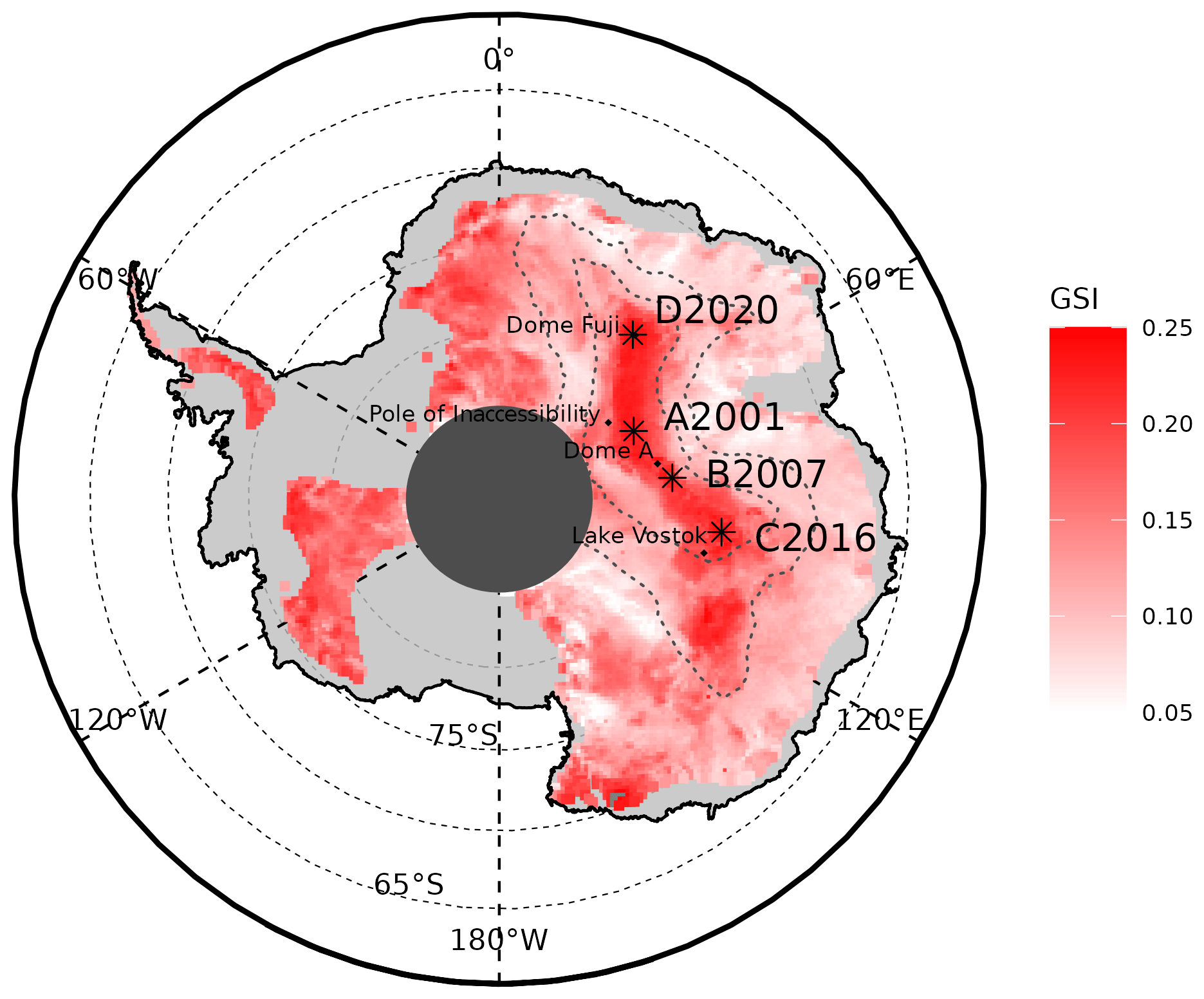
Figure 1 Map of the GSI maximum for the 2000–2022 period (colours) with the elevation contours for 3000 and 3500 m (dotted lines). The locations of the four extreme grain size events detected are marked with asterisks; the melting area is masked.

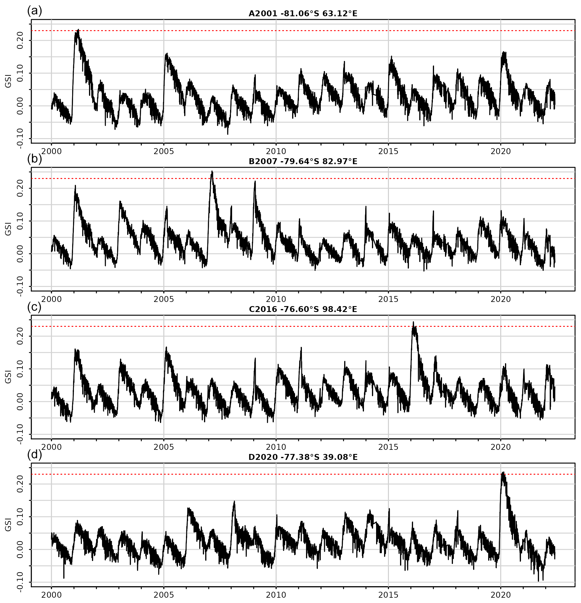
Figure 2 GSI time series for the four selected locations from January 2000 to May 2022: (a) A2001, (b) B2007, (c) C2016 and (d) D2020. The extreme growth threshold (0.23) is shown in red lines.

The SGSI is characterized by an increase in GSI of 0.14±0.01 on average with respect to the annual minimum, and it generally takes place between the end of November and the beginning of February. The following decrease in GSI tends to be slower and lasts until the next spring.

From 55 cases selected over 2000–2022 (cf. Sect. 3.2), we found that the SGSI lasts 54.9±2.4 d on average, with a minimum of 28 d and a maximum of 114 d. The mean Julian day for the onset date is 336.8±1.7 (i.e. 3 December), and for the ending date it is 25.6±2.0 (i.e. 26 January). The growing rate, defined as the total increase in GSI during the SGSI divided by its duration (in days), on average is 0.0026±0.0001 d⁻¹.

Seasonal increase in GSI is mainly driven by temperature and the subsequent increase in water vapour available to be transported within the snowpack upper layers (0–20 cm), triggering dry snow gradient metamorphism (Colbeck, 1982). Summer precipitation contributes to inter-annual variability through the deposition of a thin layer of fine grains at the surface, which increases albedo and reduces the penetration of solar radiation and the heating of the topmost layer, thereby reducing the grain growth (Picard et al., 2012). In the same way, the snow transport by wind results in a sorting of the grains by size in the topmost layers, as smaller snow grains are expected to fall out last (Grenfell et al., 1994; Domine et al., 2007). By contrast, the seasonal increase in the grains is favoured by high subsurface temperature vertical gradients (Colbeck, 1993), mainly because of the solid-state greenhouse effect (Dombrovsky et al., 2019): the snow cools at the surface by emitting infrared radiation and warms a few centimetres below by absorbing solar radiation. This effect is particularly enhanced when the sky is clear.

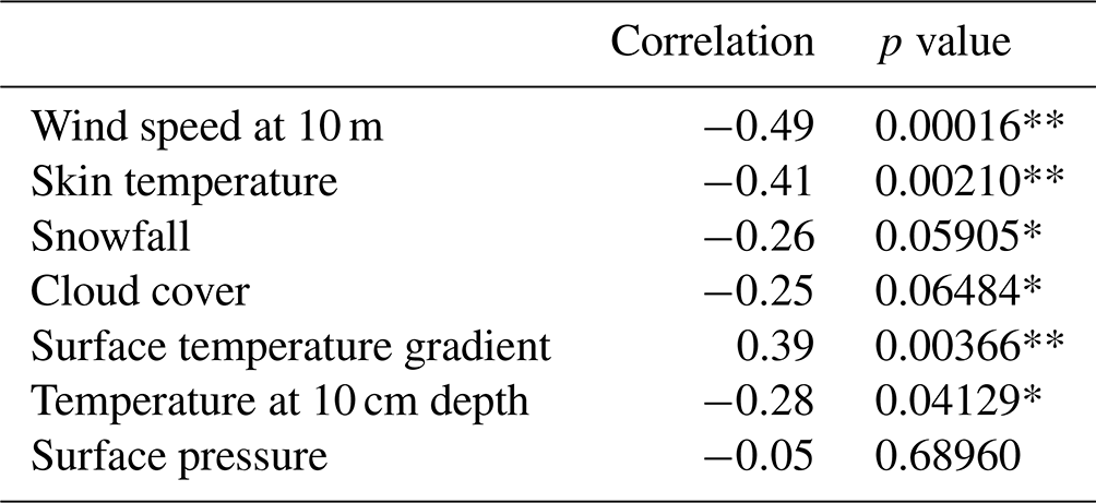
For these reasons, we analysed variations in skin temperature, surface temperature gradient, temperature at 10 cm depth, snowfall, cloud cover and wind speed at 10 m during the SGSIs in the locations of the four extreme events. Surface pressure was included to explore the possibility of a common large-scale atmospheric regime. We computed the anomaly of selected meteorological variables with respect to the 2000–2022 period, and we performed linear correlations with the seasonal maximum values of GSI. The correlation coefficients with the associated p values are reported in Table 1. For the 55 selected SGSIs, a negative significant correlation is found with skin temperature (−0.41) and 10 m wind speed (−0.49), as well as a positive significant correlation with surface temperature gradient (0.39). Thus, wind and temperature appear to be the main drivers in determining the maximum GSI. Furthermore, despite the fact the inter-annual cycle of the grain size is driven by temperature, it emerges that during the SGSI a lower-than-usual skin temperature leads to a larger grain size value.

Some weaker correlations, but significant at the 90 % level, are obtained with temperature at 10 cm depth, snowfall and cloud cover (−0.28, −0.26 and −0.25, respectively), suggesting that these factors can also be involved in the maximum GSI. Conversely, no significant correlation is found with surface pressure.

Note that Picard et al. (2012) computed correlation between the increase in GSI during 1 December–15 January and accumulated precipitation during the same period at Dome C (75.10^∘ S, 123.33^∘ E), excluding the years with accumulation larger than 4 kg m⁻². Using the same approach, we obtained a correlation of −0.30 at our four locations over 2000–2022. They found a high correlation of −0.83 at Dome C over 1999–2010, but if we extend the calculation to the period 2000–2022, we obtain a much weaker correlation of −0.44 at Dome C. Another difference is that we are using the up-to-date ERA5 reanalysis, instead of ERA-Interim (Simmons et al., 2007).

Table 1 Linear correlation coefficients between some meteorological parameters anomalies and the maximum GSI of the identified 55 SGSIs. Significance over 95 % is marked with two asterisks, and over 90 % it is marked with one asterisk.

Lastly, we studied the meteorological conditions during the SGSI onset and end by using the principal component analysis applied to the selected 55 cases, as described in Sect. 3.3. Figure 3a shows the first components for the beginning of the SGSI. GSI starts to rise around day 0, i.e. the onset date. An increase in surface pressure and in skin temperature is observed with a peak 1–2 d after the onset. The temperature gradient over the 10 cm under the surface features a decrease a few days after the onset, with a minimum at day 3, and then it increases, while temperature at 10 cm depth keeps increasing for the whole range of 30 d considered, with the maximum rate between day 0 and day 5. Snowfall has a sharp peak during day 0 and day 1, and at the same time, 10 m wind speed and cloud cover rise. Then these three parameters decrease and exhibit lower stable values after day 5. The proportions of variance explained by the first component (i.e. for each parameter the amount of its variance the first component explains) of GSI and temperatures at skin level and at 10 cm depth are high (74 %, 66 % and 95 %, respectively), but they are lower for surface pressure and surface temperature gradient (34 % and 37 %) and much lower for wind speed, snowfall and cloud cover (13 %, 26 % and 13 %, respectively). This is probably because the latter parameters have a much larger natural day-to-day variability.

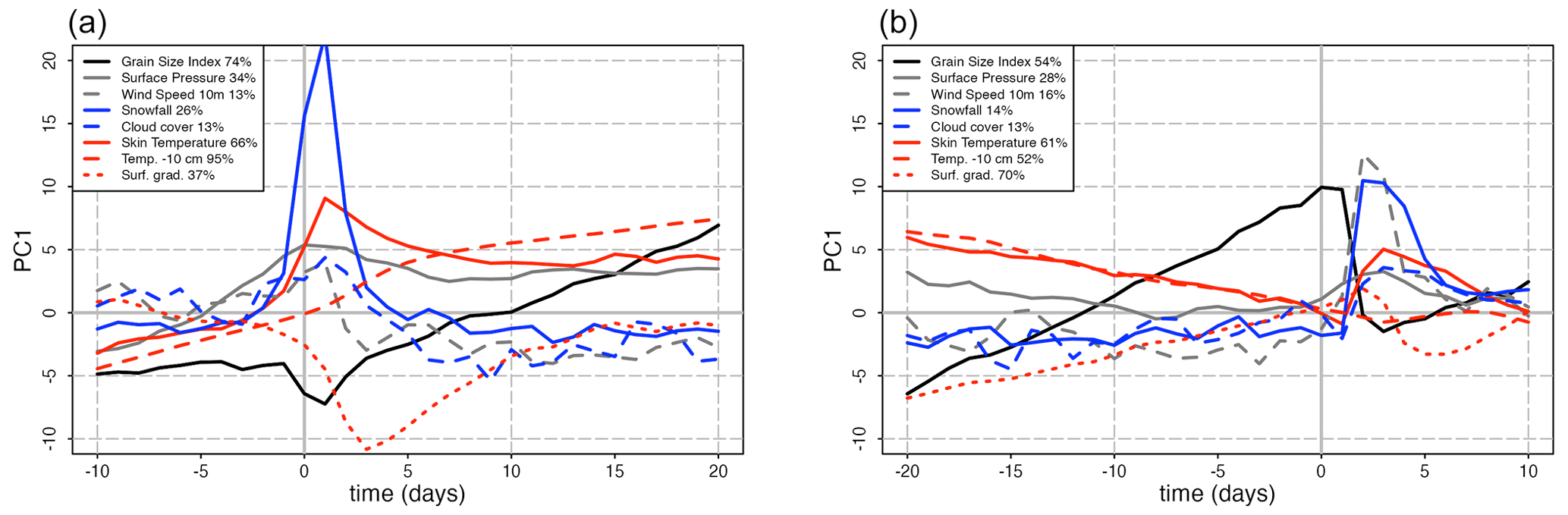
Figure 3 First components of the principal component analysis (PC1) performed over GSI, skin temperature, 10 m wind speed, snowfall, surface pressure, cloud cover, temperature at 10 cm depth, and surface temperature gradient between 0 and 1 cm in depth during (a) the onset and (b) the end of the SGSI. The proportion of explained variance for each parameter is reported in the legend.

Figure 3b reports the first components of PCA for the ending of the SGSI. GSI reaches its maximum at day 0, then sharply decreases at day 2. Note that 2–3 d from day 2, all variables change in behaviour: skin temperature and temperature at 10 cm depth show a long-term decrease, but then the first rises (during days 1–3) and the second stabilizes; the opposite variations are observed for surface temperature gradient, which exhibit a decreases during days 1–5. Snowfall, wind speed, surface pressure and cloud cover, which were low and relatively stable, have a sharp peak during days 2–3. This particular combination seems to determine the seasonal halt of the snow grain growth. The proportions of variance explained are quite similar to the onset case, with the exception of the surface temperature gradient, which is higher, while the temperature at 10 cm depth and GSI are lower, indicating a greater variability in these variables during the SGSI end. These peaks in the snowfall occurring both at the onset and at the end of the SGSI suggested exploring more details about their characteristics, as a relatively huge precipitation event could be linked to the occurrence of an AR. We investigate this in Sect. 4.3.

4.2 The four most extreme maximum grain size events

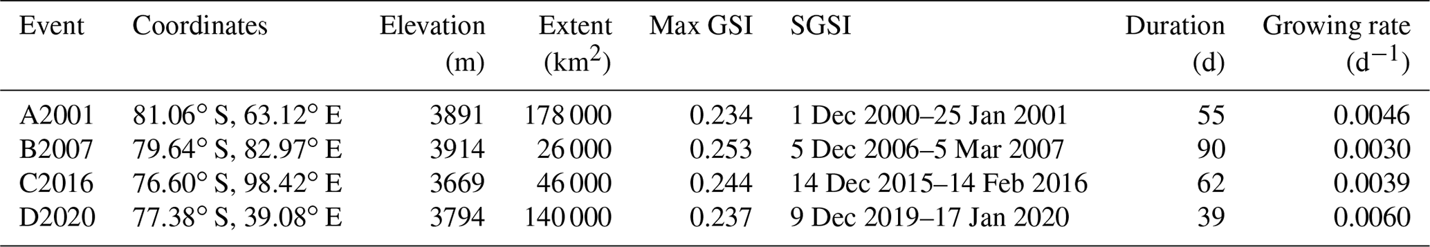
During the selected four extreme events (see Sect. 3.1), GSI increased by 0.24–0.27 between the onset and end dates and reached values above 0.23 (Table 2). Moreover, GSI remained significantly above the climatological average (2000–2022) for all of the summers and subsequent autumns, with extreme standard deviations of over +3σ during these maximums. The duration of these events ranges from 39 to 90 d.

In order to evaluate the spatial extent of the regions featuring high-GSI events, we define the extent of each of the 22 summer seasons as the area with the seasonal maximums of GSI larger than 0.20, i.e. the 95th percentile of all the maximum GSI values over the dry area in Antarctica in 2000–2022. On average, annually this area is 40 000±10 000 km².

The extent of the most extreme events ranges from 26 000 to 178 000 km². The magnitude, extent and growth rate of the A2001 and D2020 events are similar, while the B2007 and C2016 events feature a slightly larger maximum but smaller growth rate and spatial extent.

Table 2 Coordinates and elevation of the four extreme grain size events and characterization of their SGSI.

Figures 4 to 7 show GSI and some snow and atmospheric variables during the summer seasons of the most extreme events and their 2000–2022 climatology for comparison.

The A2001 event (Fig. 4) started on 1 December 2000, and the SGSI lasted until 25 January 2001. The GSI rate, defined as the daily variation averaged over a 10 d window, was maximum 1 week after the onset, when the sky was mainly clear. After the growth ending date, snowfalls became more frequent and the cloud cover and wind speed were often above the climatological mean. In February, the GSI rate was about zero and began to become negative later in March.

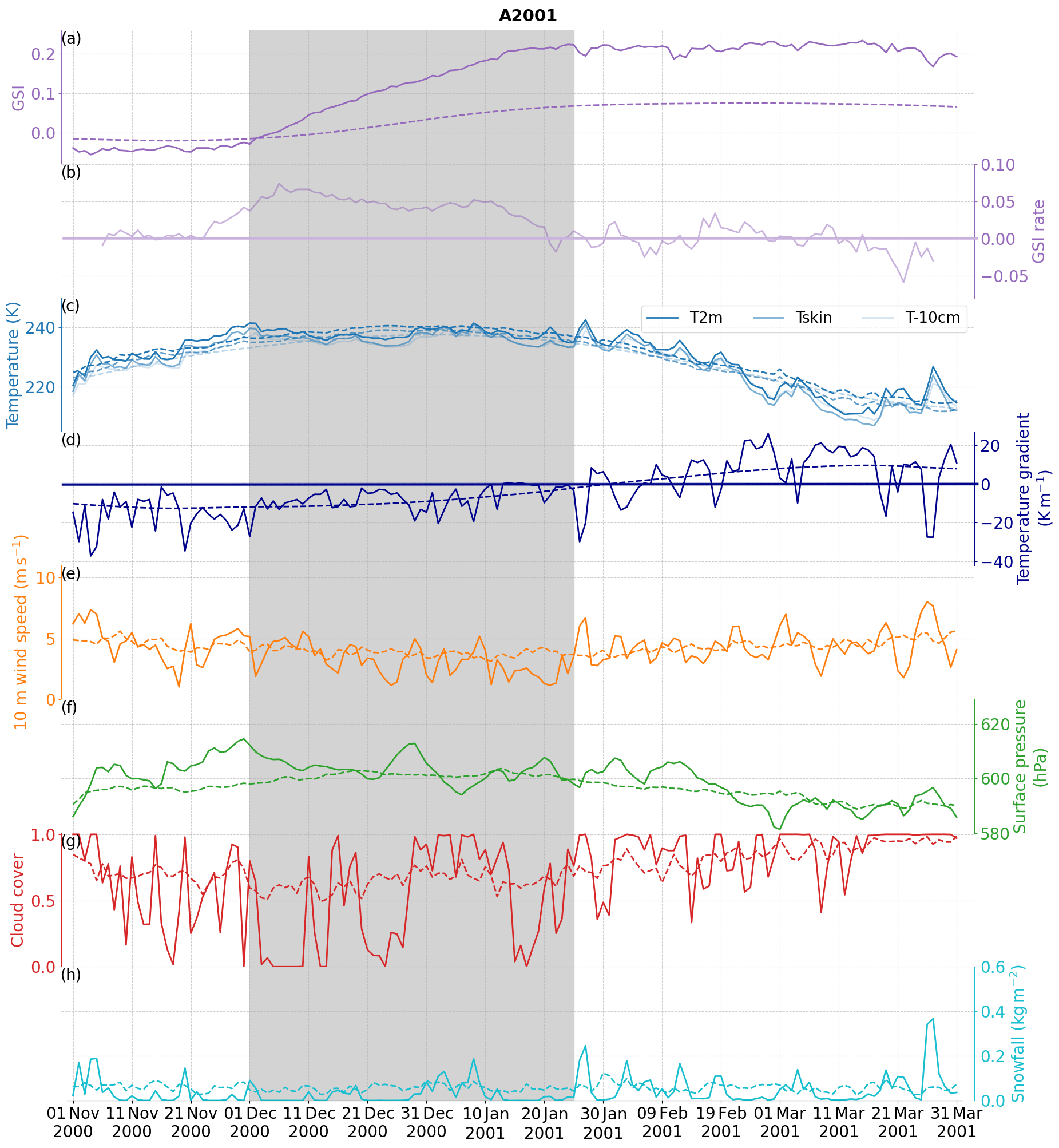
Figure 4 The A2001 event time series daily from 1 November 2000 to 31 March 2001 of (a) GSI and (b) GSI rate over a 10 d window; (c) temperature at 2 m (dark blue), skin temperature (blue), ice temperature at 10 cm depth (pale blue) and (d) ice temperature gradient between 0 and −1 cm (grey line); (e) wind speed at 10 m; (f) surface pressure; (g) cloud cover; and (h) snowfall. The 2000–2022 climatology of each variable is the dotted line. The SGSI period is in the grey area.

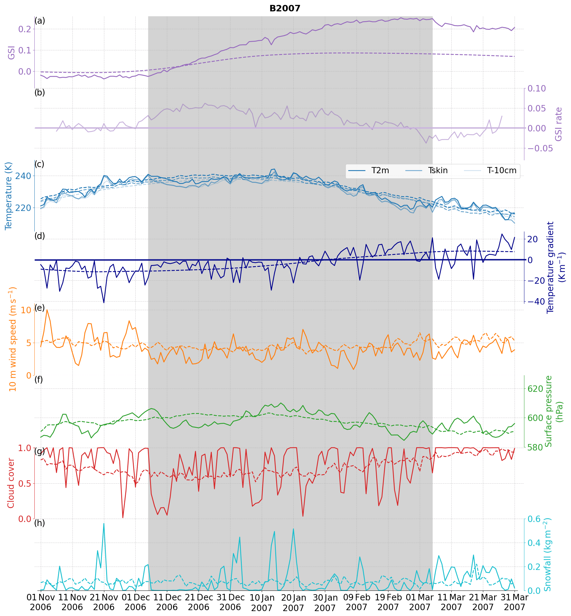
The B2007 SGSI (Fig. 5) lasted from 5 December 2006 to 5 March 2007. Despite the sudden decrease in GSI on 13 January coinciding with a large snowfall, GSI continued to increase after and the SGSI lasted 90 d, which is much longer than the mean (54.9 d; cf. Sect. 4.1) and the other extreme events (shorter than 62 d). Note that the GSI rate remained positive but decreased in January when more frequent snowfalls and higher wind speed occurred. These events differ from the other extremes by a lower mean snowfall anomaly of nearly zero during the SGSI (−3 % with respect to the 2000–2022 climatology, compared to −50 % or below for the other extreme events). Besides this, excluding the days immediately after the onset, the sky was generally cloudy during the whole SGSI (a non-significant +2 % in total with respect to climatology during the SGSI, while the anomalies for the other extremes were negative, from −7 % to −23 %).

Figure 5 As in Fig. 4 but for the B2007 event, from 1 November 2006 to 31 March 2007.

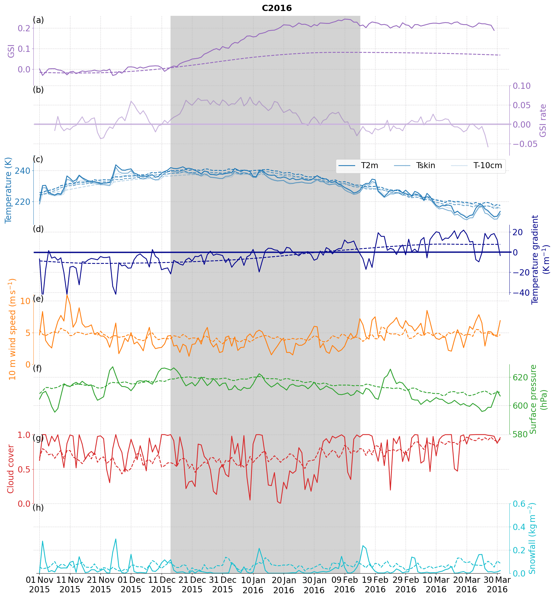
The C2016 event (Fig. 6) started on 14 December 2015 and stopped on 14 February 2016. The GSI rate was steadily positive until mid-January and then began to decrease. The wind was generally below the climatological mean, and snowfalls were scarce. Starting from the end date, when a snowfall occurred, the wind speed suddenly rose above average and remained steadily high.

Figure 6 As in Fig. 4 but for the C2016 event, from 1 November 2015 to 31 March 2016.

Finally, the onset date of the D2020 event was 9 December 2019 (Fig. 7), and GSI increased until 17 January 2020. The GSI rate was high (nearly +0.1 per 10 d) from the onset to the end of December, and the growing rate averaged over the SGSI was the highest of all extreme events (see Table 2). The condition of low wind speed around the onset was favoured by a high-pressure situation, above the climatological mean by nearly 20 hPa in the days right before the onset (the highest value among the extreme events). Overall, the condition of calm wind was maintained for the rest of the SGSI, recording the largest negative anomaly (−0.8 m s⁻¹) among the extreme events. The onset occurred just after a large precipitation event observed over the 8–10 December period (1.1 kg m⁻² of snowfall), while the other extreme events had smaller accumulations around the onset. Note that snowfall amounts on 8 and 9 December 2019 were both above 0.4 kg m⁻², corresponding to a precipitation event ranking above the 95th percentile for daily snow accumulation as estimated by Dittmann et al. (2016). Very little snowfall was recorded during the rest of the SGSI. The wind speed increased at the SGSI end, and in the following days wind speed above the climatology often occurred accompanied by snowfalls.

Figure 7 As in Fig. 4 but for the D2020 event, from 1 November 2019 to 31 March 2020.

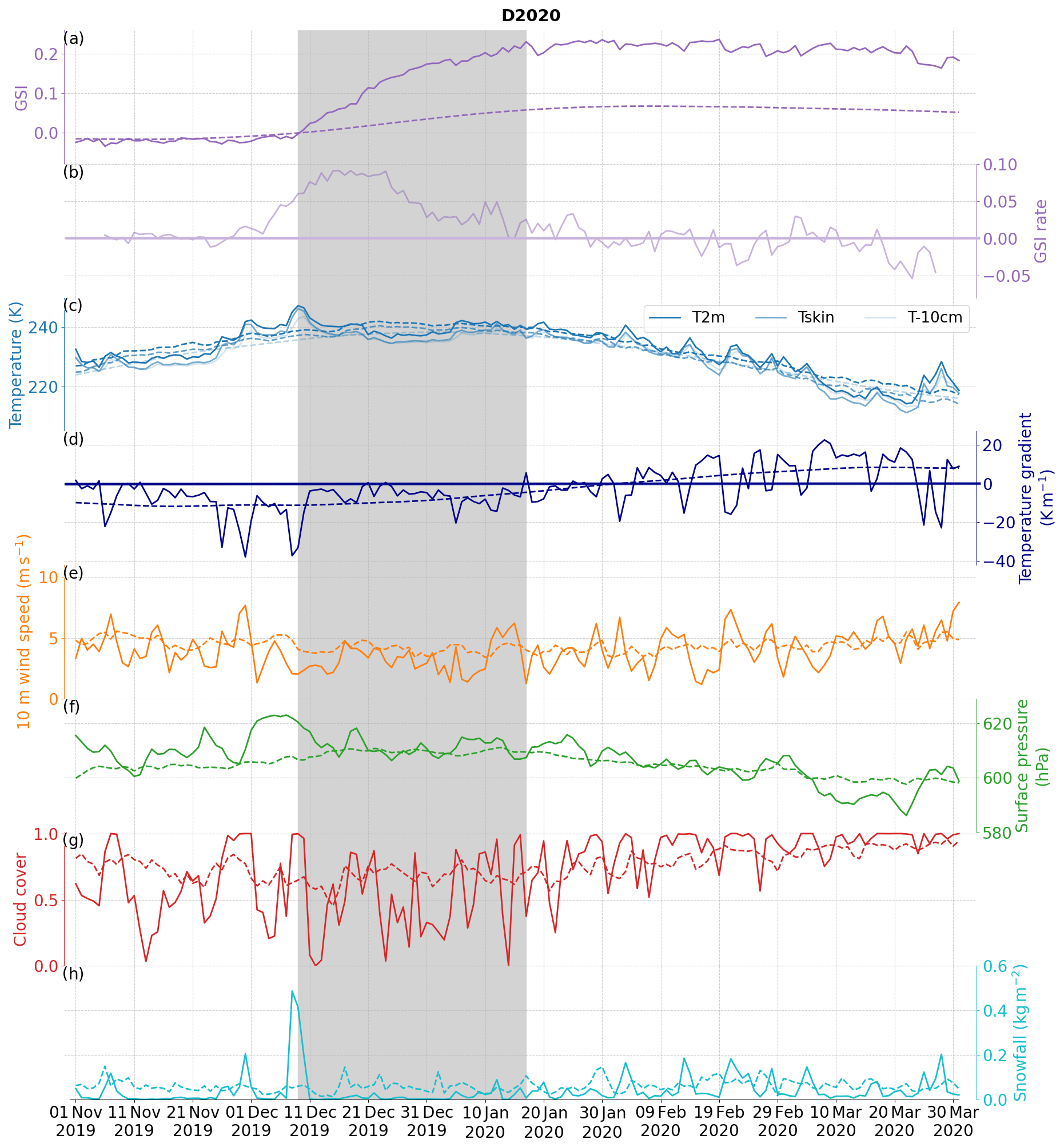
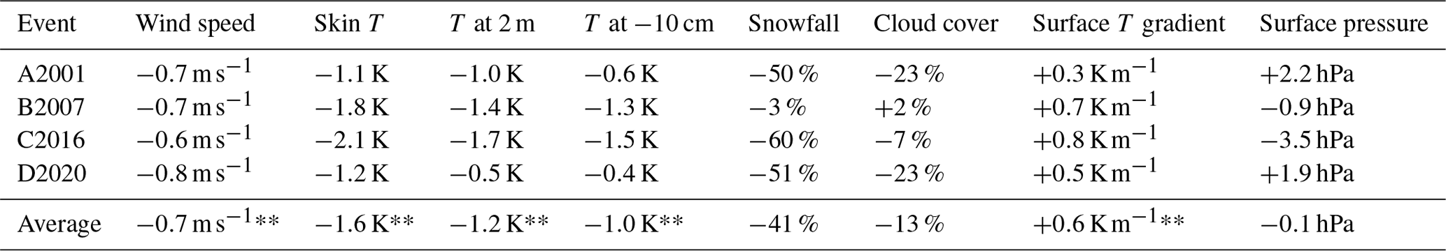
Table 3 summarizes the anomalies in wind speed at 10 m, various temperatures, snowfall, cloud cover, surface temperature gradient and surface pressure during the SGSIs of the four most extreme grain size events. Even though these four cases had different durations, some common features appear: the presence of snowfall precludes the onset accompanied by negative surface temperature gradients; a condition of low wind speed for a few days following the onset, also with low temperatures, especially at skin level; and very few snowfalls and low cloud cover, except for the B2007 event (Fig. 5), which had frequent snowfall events. No clear conclusion can be drawn for the surface pressure anomaly, since two events occurred with positive mean anomalies and two events occurred with negative ones. However, in the 10–15 d around the onset, the pressure anomaly was positive in all cases.

Table 3 Mean anomalies with respect to the 2000–2022 climatology during the SGSIs of the most extreme events. Significance over 95 % is marked with two asterisks.

4.3 On the role of atmospheric rivers

The SGSI onset and end are generally associated with stormy conditions inducing large precipitation amounts, as shown in Fig. 3. Recently, Wille et al. (2021) demonstrated that ARs, which facilitate the intrusion of relatively warm and moist air masses from the lower latitudes into Antarctica, generate extreme snowfall events. They also play a leading role in determining the Antarctic precipitation variability on inter-annual timescales, especially on the East Antarctica Plateau where the snowfall accumulation is overall low. They estimated that, in spite of their rareness (about 1 % of the time), ARs are responsible for around 10 %–20 % of the annual accumulation across East Antarctica. Along the highest East Antarctic ice divide, large amount of snow can be generated under blocking anticyclonic circulations or ridging situations which channel the moist air from the mid-latitudes southwards, towards the interior (Hirasawa et al., 2013; Pohl et al., 2021).

Here, we study the possible link between the presence of ARs and the SGSI. Assessing the co-occurrence of ARs and the onset date requires comparing their frequency around the onset date and performing a statistical test to determine if this frequency is significantly different from that obtained with random dates (cf. Sect. 3.4).

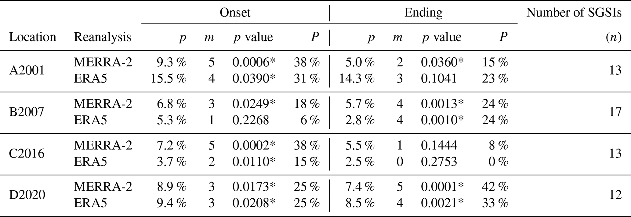
In Table 4, for each AR catalogue and location, we reported the number of onsets available for each location (n), the frequencies of AR occurrence in 1000 random 5 d intervals centred between November and December in 2000–2022 (p), and the number of onsets associated with at least one AR in the 5 d window centred on each onset (m). m values are compared to a binomial distribution with n and p, and the p values are in Table 4. Between 2000 and 2022, the onsets and ARs are very unlikely to be independent, except at the B2007 location where the relationship using the ERA5 catalogues is not statistically robust. Thus, we can reject the null hypothesis that ARs and the onset of the grain SGSI are independent. However, the onsets are not associated with an AR. For the four locations, the probability that ARs are associated with an onset ($P=m/n$) is ∼19 % and ∼30 % on average for ERA5 and MERRA-2, respectively (Table 4). Additionally, no AR approached the four locations during the onset of the most extreme SGSIs investigated in Sect. 4.2. Note that some discrepancies exist between reanalysis in Antarctica due to the scarce observations available to constrain the models by assimilation. But the fact that the two reanalyses provide convergent results suggests that the signals are robust and reproducible. Therefore, ARs are sometimes involved in the onset, but they are not a necessary condition, and they do not play a role in determining the maximum seasonal grain size. Similar analyses were conducted to assess the co-occurrence of ARs and the end date of the SGSIs (Table 4) considering the months between January and March in 2000–2022. At least in two or three of the four locations, there is a significant connection between ARs and the ending of the SGSI, with the probability that ARs are associated with the ending dates being ∼20 % and ∼22 % on average for ERA5 and MERRA-2, respectively, but with larger variability with respect to the onset case.

Table 4 Statistical parameters used in a binomial distribution to assess the significance of the co-occurrence of the ARs and the onset and ending dates. The meaning of each parameter is explained in the text. The p values over 95 % are marked with an asterisk.

5 Discussion

5.1 Grain growth

Our analysis shows that the amplitude of the summer increase in GSI is highly variable, and large anomalies emerge occasionally during the summer, giving rise to very high values of grain size, localized in specific areas. We found some interactions between grain size evolution and local meteorological conditions at different timescales, from daily to seasonal, along the main East Antarctic ice divide. Wind and skin temperature have been shown to play a leading role in affecting snow metamorphism during the austral summer with significant correlation with GSI. We observed that the beginning of the growth usually takes place just after a snowfall: at first, the grain size decreases during the precipitation, as new smaller grains are brought onto the surface (Domine et al., 2007). However, the snowfall is usually associated with a large near-surface temperature gradient which is a driver of the dry snow metamorphism causing a rapid increase in the grain size (e.g. Colbeck, 1982; Grenfell et al., 1994).

The East Antarctic Plateau cannot be regarded as thermally homogeneous (González et al., 2021). For instance, katabatic winds transport cold air downhill from the domes and the ice divides, and shallow depressions exist on the flank of the ice divides where pooling of drained cold air allows for greater radiative heat loss and hence enhanced cooling of the surface (Scambos et al., 2018). Besides this, because of their top positions, the ice divides are characterized by a general wind divergence (Parish and Bromwich, 2007) and weak wind conditions (Yamanouchi et al., 2003). In addition to the low accumulations, these features are favourable to the presence of large snow grains since high-speed winds tend to transport and deposit small ice particles on the surface, burying larger grains present. Moreover, lower-than-normal skin temperature observed during the SGSIs of the most extreme events, suggests that a large temperature gradient is possible in the first centimetres of the snowpack and hence an enhanced flux of water vapour could appear from the subsurface to the surface, leading to the formation of recrystallization crystals (Flanner and Zender, 2006; Champollion et al., 2013; Leduc-Leballeur et al., 2017). Cold surface conditions could result from the conditions of a generally clearer-than-normal sky observed during these phases, favourable to local intense radiative cooling of the surface and an enhanced solid-state greenhouse effect (Dombrovsky et al., 2019), causing a strong thermal gradient in the uppermost part of the snowpack, as observed in Gallet et al. (2014). The solid-state greenhouse effect could not be appreciated in this study as we used the Python version of the MFM, in which its parameterization is absent. The low wind speed also hinders the dispersion into the atmosphere of the sublimated snow favouring local supersaturation conditions and, hence, the growing of grains.

5.2 Link with large-scale mean conditions

As demonstrated by Wille et al. (2021), the zonal distribution of the 500 hPa geopotential height anomalies associated with ARs landfalls resembles the negative phase of the SAM. We thus analysed if a possible connection between GSI increase and large-scale atmospheric circulation also exists. The 500 hPa geopotential height can help identify large-scale atmospheric structures, such as the tropospheric polar vortex (Kwon et al., 2020; Gordon et al., 2022). Figure 8 shows the mean standardized anomalies of ERA5 500 hPa geopotential height (with respect to 2000–2022 climatology) for the 5 d intervals centred on the available onset dates for each location. There are mostly positive anomalies all over the continent, with significant values in the area near the considered locations, with waviness in the Southern Ocean. The same analysis was performed using the MERRA-2 reanalysis dataset and provided similar results (not shown). For the four study cases, we also observe a positive anomaly in the Amundsen Sea, possibly related to a low activity of the Amundsen Sea Low (see for example Turner et al., 2012).

Some tests were performed in order to assess a more frequent occurrence of particular zonal wavenumbers during the 55 onsets, but the results were not conclusive. Transient waviness (wavenumber 3 or 4) can be seen in Fig. 8, though not at significant level; hence future work will study in more detail the possible involvement of mid-latitude atmospheric dynamics and zonal wave activity.

In Fig. 8 we can observe, in all the four cases, that there are some pressure differences between the continent and the ocean that are clearly reminiscent of the SAM. Thus, these seasonal events of grain size increases tend to correspond to negative SAM-like patterns. Further analysis of the Antarctic Oscillation index shows that the period October–December 2019 (the months before the D2020 event) recorded the lowest mean value of the AAO index since the beginning of this time series in 1979 (Lim et al., 2021). This was the result of a minor sudden stratospheric warming (SSW) that occurred in September 2019 and propagated downwards, thereby causing anomalous tropospheric circulation from the end of October to mid-December 2019 (Shen et al., 2020). Such SSW events are very rare in the Southern Hemisphere, as their occurrence has been estimated as 4 % per year (Wang et al., 2020). However, this did not happen before the other three extreme snow grain size events. During the four most extreme events most of the time (three cases out of four) a negative AAO index is present, i.e. a weak polar-vortex situation. In particular during the 5 d intervals centred on the onsets of the four most extreme events we find an average of the AAO index of −1.48 (A2001), 0.18 (B2007), −1.71 (C2016) and −2.09 (D2020). A negative AAO situation seems to favour the SGSI. However, a negative AAO is neither necessary nor sufficient. It is not necessary as other onsets had very negative AAO values (not shown) and they did not ended in a high GSI later in the season. It is not sufficient since the AAO index for the B2007 event is slightly positive. In fact, over the 55 selected cases, 31 had negative AAO mean values in the 5 d intervals centred on the onsets, with an average of $-\mathrm{0.39}\pm \mathrm{0.19}$ over all the cases, with a p value of 0.078 on a two-tailed t test. Thus, a negative AAO index is more present than the positive phase during the onsets, even though this does not reach the 95 % significance level.

In the Dome Fuji area during the anticyclonic circulation, a peculiar situation of a warm-core eddy emerges near the top of the dome, while cooler air accumulates on the saddle on the eastern side, as described in Sect. 5.1. Indeed, on 5 December 2019, ERA5 reanalysis recorded the maximum gradient of about 4 K between the warm-core eddy and the saddle. Afterwards, temperature dropped until the beginning of January 2020, with an average anomaly of −4.3 K from 21 December 2019 to 4 January 2020, also observed in Fig. 7. The anticyclonic ridge developed when an intense wet oceanic airflow arrived over the ice sheet plateau through the Dronning Maud Land on 7–9 December and reached Dome Fuji, which became the centre of the anticyclonic anticlockwise rotation of the flow. This event is not an AR according to the criteria defined in Wille et al. (2021), and neither is the A2001 nor B2007 event, when moisture intrusions arrived from Enderby Land and Amery Ice Shelf, respectively. Only the C2016 event is associated with an AR occurrence, which arrived from Victoria Land, on the basis of the ERA5 catalogue but not of the MERRA-2 catalogue. Nonetheless, intense moisture advections were present during all these extreme events.

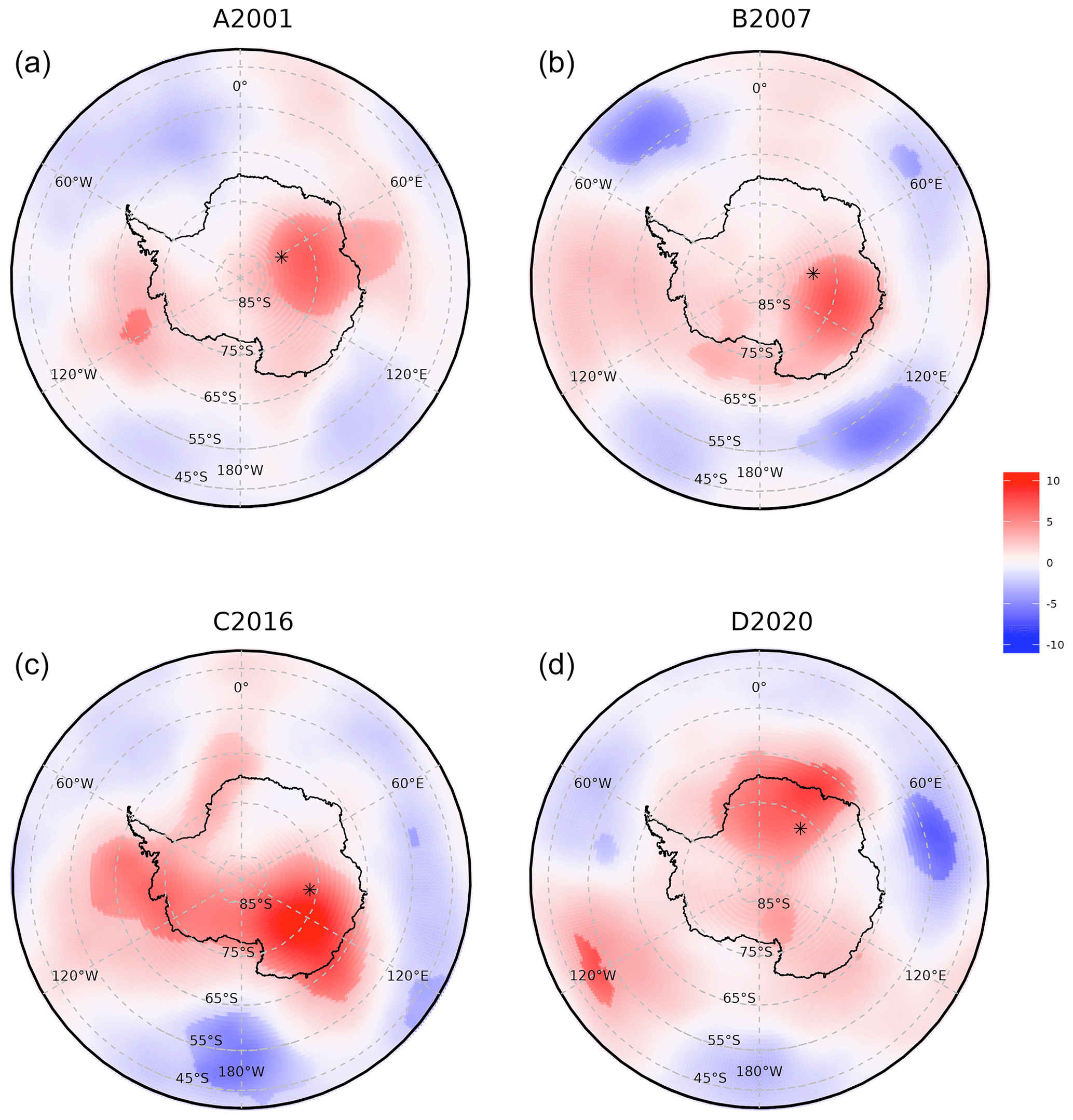
Figure 8 Mean anomalies of the 500 hPa geopotential height fields from ERA5 over the period between 2 d before and 2 d after each synchronized onset date available for each location with respect to the 2000–2022 climatology. The number of available onset dates are 13, 17, 13 and 12, respectively. Brighter colours highlight the value with a significance over 90 %. Asterisks mark the locations of (a) A2001, (b) B2007, (c) C2016 and (d) D2020.

6 Conclusions

We studied the seasonal variations in the grain size in East Antarctica using an index computed using the 150 and 89 GHz observations from the satellite instrument AMSU-B and previously introduced and analysed at Dome C (Picard et al., 2012). The present study covers the interval 2000–2022, the entire period of availability of the remotely sensed snow grain size index from AMSU-B sensors, over which we identified 55 seasonal grain size increases (SGSIs) in four locations with identifiable onset and end dates. Using the ERA5 reanalysis, we established that grain size signal is linked to particular atmospheric conditions. In order to study these favourable circumstances, we identified four events of extreme increase in the grain size, in different locations along the highest ice divide, and compared them to the usual SGSIs between 2000 and 2022. We searched for connections with local meteorological conditions and then with the synoptic atmospheric background.

The growth onset of the snow grains is usually linked to a snowfall event in one-third or one-fifth (according to MERRA-2 and ERA5, respectively) of the considered 55 cases associated with the presence of an atmospheric river providing warm and moist air into the inner plateau. The final maximum value of the grain size, which is usually reached in January–February, is determined by what happens in the weeks following the onset: the common features during the SGSI which emerge from this study are conditions of low wind speed and skin temperature below the climatological mean.

We observed that ARs and, to a lesser extent, weak polar-vortex conditions were related to the SGSI onset and end. However these situations are not necessary conditions. Another potential connection may exist with the Amundsen Sea Low, but our study did not allow for accurately characterizing if a co-occurrence of different critical conditions could provoke a large GSI event. Further analysis could be done using the ERA5 reanalysis in order to extend the time interval and evaluate the significance of these anomalous situations and possibly to discover some other similar configurations which had led to intense growth of the snow grain. The microwave data available in the past (e.g. Special Sensor Microwave/Imager, SSM/I) miss the 150 GHz channel, but the 85–91 GHz channel could be used to find abrupt decreases in 1987–1999. However, the extension is not trivial as the grain size index is indirect and results from remote sensing observations. In situ observations should be included in the analysis, when available, in order to correct possible biases.

This analysis allowed for improving the understanding of the causes of the SGSI onset and end and could be important for projections of the frequency of extreme GSI events in a changing climate.