Linking glacier retreat with climate change on the Tibetan Plateau through satellite remote sensing

Under global climate change, glaciers on the Tibetan Plateau are experiencing severe retreat, which significantly impacts the regional water cycle and the occurrence of natural hazards. However, detailed insights into the spatiotemporal patterns of this retreat and its climatic drivers remain insufficiently explored. In this study, an adaptive glacier extraction index (AGEI) is proposed based on the analysis of multispectral Landsat images integrated with the Google Earth Engine, and comprehensive and high-resolution mapping of glaciers on the Tibetan Plateau is realized at 5-year intervals from 1988 to 2022. Subsequently, the ERA5-Land air temperature and precipitation data are downscaled to a finer 1 km resolution. Finally, the impacts of the annual and seasonal changes in the downscaled meteorological factors on the glacier extent are quantified. Results demonstrate a rapid yet heterogeneous pattern of glacier retreat across the Tibetan Plateau between 1988 and 2022, with retreat rates ranging from 0.14 ± 0.07 % to 0.51 ± 0.09 % annually. A notable trend is observed: most glaciers experienced a decrease in extent from 1990 to 2000 followed by a slight increase from 2000 to 2010. From 2010, a majority of the glaciers exhibited either a static state or minimal retreat. The most pronounced impact of annual temperature on glacier retreat is observed in the southern Himalayas, with a value of −9.34 × 10³ km² °C⁻¹, and the most restraining impact of precipitation on glacier retreat reaches 261 km² mm⁻¹, which is observed in the Karakoram Range for the spring season. These insights are pivotal in comprehending the temporal and spatial heterogeneity of glacier retreats and in understanding the effects of climatic variations on the state of glaciers on the Tibetan Plateau.

1 Introduction

The Tibetan Plateau, often referred to as the Third Pole, hosts the largest concentration of glaciers outside of the polar regions (Yao et al., 2012). These glaciers are integral to the regional water cycle and are a vital source of water for downstream areas (Zhang et al., 2021; Salerno et al., 2023). However, the current glacier mass balance has indicated severe glacier retreat (excluding the Karakoram anomaly) at an accelerated rate, and this has primarily been attributed to climate warming (Curio et al., 2015; Farinotti et al., 2020; Zhang et al., 2021; Chen et al., 2023). Prior research on High Mountain Asia documented that the region's glacier area experienced a reduction of 0.43 ± 0.19 % yr⁻¹ from 1990 to 2018, and the glacial mass loss was quantified at 16.3 ± 3.5 Gt yr⁻¹ between 2000 and 2016 (Brun et al., 2017; Huang et al., 2021). This pronounced glacier retreat has resulted in considerable alterations to runoff patterns on seasonal, interannual, and decadal scales. Concurrently, there is an escalating risk of glacial hazards, including avalanches, glacial debris flows, and glacial lake outburst floods. These developments pose a significant threat to life and property across the region (Lamsal et al., 2016; Lin et al., 2021; Zhao et al., 2022).

Glacier change can be measured using variations in area, thickness, volume, surface mass balance, and equilibrium-line altitude (Sugiyama et al., 2013; Su et al., 2022). These parameters can be monitored for individual glaciers via geodetic and glaciological techniques (Zemp et al., 2019). The advent and enhanced accessibility of high-resolution, high-quality satellite imagery have enabled comprehensive investigations of glacier changes on a regional scale (Che et al., 2020; Beraud et al., 2023). Over recent decades, the focus on the Tibetan Plateau has been towards conducting glacier mapping and change analyses at the basin level, utilizing satellite remote-sensing data (Wang et al., 2013; Neckel et al., 2014; Ye et al., 2017; Zhang et al., 2021). Glaciers are commonly mapped using a variety of techniques, including spectral analysis of optical satellite images (Bolch et al., 2010), object-segmentation-based methods (Robson et al., 2015), and supervised machine learning algorithms (Khan et al., 2020). Additionally, synthetic aperture radar (SAR) coherence images are being increasingly utilized for glacier mapping, leveraging their ability to penetrate cloud cover (Holobâcă et al., 2021). Among these methods, robust and efficient pixel-based multispectral analysis has been particularly effective with respect to accurately delineating debris-free glaciers (Huang et al., 2021). This approach harnesses the distinct spectral signatures of ice and glaciers, allowing for precise identification and mapping of glacier boundaries (Huang et al., 2021; Bevington and Menounos, 2022). However, the magnitude of glacier retreat on the Tibetan Plateau varies significantly, influenced by marked spatiotemporal variations in climate conditions and topographical factors (Ye et al., 2017; Latif et al., 2019). Furthermore, limited by the large number of satellite images and massive computing requirements, the comprehensive depiction of glacier retreat across the entire Tibetan Plateau, especially at finer temporal and spatial resolutions, remains inadequately characterized (Shean et al., 2020; Xiao et al., 2023). Recent advancements in cloud computing platforms, such as Google Earth Engine, have significantly enhanced automated glacier-mapping capabilities. By harnessing extensive archives of satellite imagery, the Google Earth Engine platform facilitates a more comprehensive understanding of the impacts of global climate change on the cryosphere (Gorelick et al., 2017; Shugar et al., 2020; Huang et al., 2021; Bevington and Menounos, 2022).

Generally, regional climatic conditions determine the intensity of glacier ablation and accumulation (i.e., mass balance) over prolonged periods, and climate change, especially increasing temperature, is recognized to be the dominant driver of glacier mass balance and the associated area and volume changes (Su et al., 2022). Glaciers serve as sensitive indicators of climate, primarily responding to interannual variations in temperature and precipitation (Harrison, 2013; Shean et al., 2020). One critical challenge in understanding glacier responses to climatic changes is the significant variability in glacier sensitivities. These sensitivities and the associated feedback mechanisms can either accelerate or restrain glacier melting (Johnson and Rupper, 2020). Consequently, the availability of high-resolution meteorological data becomes essential for accurately discerning the patterns and dynamics of glacier retreats in response to climate change (Rashid and Majeed, 2018). Obtaining high-resolution gridded meteorological data at a regional level typically involves interpolations of rain gauge observations and satellite estimates (Crespi et al., 2019; Afonso et al., 2020). However, the applicability of these methods is often limited in complex terrain, primarily due to the sparse observations and their inherently coarse spatial resolutions. Statistical downscaling techniques are routinely applied to refine the spatial resolution of temperature and precipitation datasets by leveraging ancillary variables available at finer scales (Ebrahimy et al., 2021; Jiang et al., 2021). Research has consistently demonstrated a correlation between climatic variables and a range of biophysical factors, including topography, land cover types, vegetation cover, surface albedo, and soil moisture status (Hutengs and Vohland, 2016; Zhang et al., 2019). The integration of these high-resolution ancillary variables enables the production of more detailed meteorological products, thereby providing a more accurate representation of local climatic conditions, which is essential for various environmental assessments. Moreover, meteorological reanalysis datasets, such as ERA5-Land, are continually updated, thereby facilitating analyses of climate trends and anomalies. These datasets can be effectively utilized as climate inputs for downscaling analyses (Muñoz-Sabater et al., 2021; Wang et al., 2021; Kusch and Davy, 2022; Salerno et al., 2023).

Despite numerous studies examining glacier variations on the Tibetan Plateau in recent decades (Yao et al., 2012; Neckel et al., 2014; Ye et al., 2017; Bibi et al., 2018; Sun et al., 2018; Latif et al., 2019; Zhang et al., 2021; Xiao et al., 2023), the specific impacts of climate change on changes in the glacier extent have not been thoroughly investigated at a finer resolution. This study is designed with three primary objectives: (1) production of a high-resolution map of debris-free glaciers on the Tibetan Plateau, capturing changes at 5-year intervals from 1988 to 2022; (2) acquisition of downscaled meteorological products, to enhance the spatial resolution of climatic data; and (3) quantification of the impacts of annual and seasonal climate change on the patterns and rates of glacier extent change.

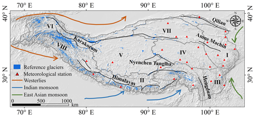
Figure 1 Delineation results for the eight subzones on the Tibetan Plateau and the reference glaciers obtained from the Randolph Glacier Inventory (RGI) 7.0. The background image is the topographic map from the Shuttle Radar Topographic Mission (SRTM) digital elevation model (DEM) provided by the USGS EROS Archive (EROS Centre, 2018).

2 Study area

The Tibetan Plateau, encompassing an expansive area of approximately 3 × 10⁶ km² and characterized by an average elevation of about 4300 m, has witnessed notable climatic shifts in recent decades (Royden et al., 2008; Zhang, 2019). The region has experienced a pronounced warming trend, with air temperatures rising approximately 0.3–0.4 °C per decade over the past 50 years. Concurrently, there has been a marginal yet observable increase in precipitation levels across the plateau (Bibi et al., 2018; Zhang et al., 2021). As shown in Fig. 1, the atmospheric circulation patterns on the Tibetan Plateau are predominantly governed by the interplay between the East Asian and Indian monsoon systems during summer and the influence of midlatitude westerlies during winter. These circulation patterns, in conjunction with distinct topography, exert a significant influence on the climatic factors that control the variability and distribution of glaciers (Yao et al., 2012). The intricate dynamics of these atmospheric systems, coupled with the unique geographical features of the plateau, play a crucial role in shaping the climatic conditions that directly impact glacier behavior and distribution (Sun et al., 2018).

To systematically evaluate the status of glaciers and comprehend the influences of climate change on their retreat, the Tibetan Plateau is divided into eight distinct subzones. This division primarily hinges on the patterns of large-scale atmospheric circulation, as shown in Fig. 1. In addition, the delineation of these subzones incorporates considerations of the drainage basins. This process is further refined using the HydroBASINS dataset (https://www.hydrosheds.org/, last access: 30 November 2024), which aids to ensure accurate differentiation of the subzones. Depicted in Fig. 1 are the delineation results of the eight subzones. Zones I, II, and VI are predominantly influenced by the East Asian monsoon, Indian monsoon, and westerlies, respectively. Zone III experiences impacts from both the East Asian and Indian monsoons, while the interplay of the westerlies and the East Asian monsoon governs Zone VII. Similarly, Zone VIII is under the influence of both the westerlies and the Indian monsoon. Zone IV occupies the transitional area between the East Asian and Indian monsoons, whereas Zone V is situated in the transitional zone between the westerlies and the Indian monsoon.

This research utilizes the Randolph Glacier Inventory (RGI) 7.0 as the reference for glacier outlines (RGI 7.0 Consortium, 2023). The RGI 7.0 is compiled through a combination of manual and automated digitization. Figure 1 illustrates that the majority of glaciers cataloged in the RGI 7.0 are concentrated in zones II, VI, and VIII, predominantly situated in the Karakoram Range and the Himalayas. The glaciers on the Tibetan Plateau, occupying diverse terrain conditions, distinctly reflect the variations in atmospheric circulation processes.

3 Data and methods

3.1 Glacier mapping using Landsat image time series

The time series of multispectral satellite images utilized for glacier mapping encompasses data from the Landsat 4 and Landsat 5 Thematic Mapper (TM), Landsat 7 Enhanced Thematic Mapper Plus (ETM+), and Landsat 8 Operational Land Imager (OLI) sensors. The Landsat data are used via the Google Earth Engine platform and are chosen due to their prolonged data availability period and comparatively high spatial resolution. The identification of debris-covered glaciers from satellite imagery poses significant challenges, as distinguishing debris from snow and ice is feasible only when glacier boundaries are predefined (Robson et al., 2015; Huang et al., 2021). Thus, this study focuses solely on debris-free glaciers. In this study, an adaptive glacier extraction index (AGEI) method is proposed to accomplish the mapping of debris-free glacier time series. The AGEI method is primarily based on the analysis of the normalized difference snow index (NDSI). Numerous studies have demonstrated the efficacy of the NDSI with respect to distinguishing glacier ice from non-ice areas, particularly in shadowed regions (Burns and Nolin, 2014; Huang et al., 2021; Bevington and Menounos, 2022). Nevertheless, the potential for misidentification persists, primarily due to factors like glacial lake presence and seasonal snow cover. To reduce such errors, the AGEI method also encompasses the normalized difference water index (NDWI) and the surface temperature. The proposed AGEI method for glacier mapping is delineated in the following three steps:

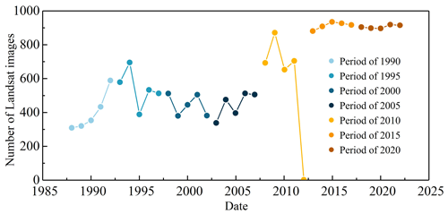
Figure 2 Number of Landsat images with less than 60 % cloud cover for each year corresponding to each period of glacier mapping.

1. Generation of Landsat data cube at 5-year intervals spanning from 1988 to 2022.

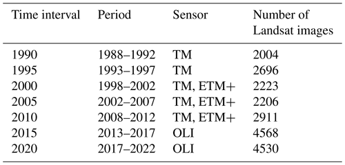
   Obtaining cloudless Landsat images on the Tibetan Plateau presents significant challenges, primarily due to the impact of shadows at low sun angles and the relatively short duration of the snow-free season (Liu et al., 2020). To mitigate the influence of clouds and seasonal snow on glacier mapping, this study uses the data cube from the Landsat data collection, and the acquisition dates of the atmospherically corrected Landsat images are restricted to the ablation season (from 1 June to 31 August). Subsequently, the cloud score is calculated for each pixel in the data cube, ranging from 0 (indicating cloud-free) to 100 (representing very thick cloud cover). In this study, the cloud score threshold is set to 60, balancing the need for a sufficient number of image pixels against the accuracy of the mapped glaciers. In addition, the quality of Landsat images is affected by cloud cover, and the Landsat images in 1 year may not generate a relatively cloud-free image mosaic. Although there may be large interannual variability in glacier area, this study analyzed the changes in glacier extent for every 5-year interval to increase the number of Landsat images and to improve the robustness of changes in glacier extent. The acquisition dates and the corresponding number of available Landsat images used for each glacier map are detailed in Table 1. Furthermore, the number of Landsat images with less than 60 % cloud cover for each year corresponding to each period of glacier mapping is depicted in Fig. 2. It can be seen that the number of Landsat images per year corresponding to each period is relatively evenly distributed except for the period of 2010. In particular, the number of Landsat images in 2012 was zero, which can be attributed to the data availability of Landsat 5 from March 1984 to May 2012. In addition, the Landsat 8 mission was successfully launched in February 2013; thus, the number of available Landsat images has increased since 2013.

2. Establishment of the AGEI utilizing the Landsat data cube

   In this study, the AGEI is established based on analyses of the NDSI, NDWI, and surface temperature. The NDSI is calculated as the difference between the reflectances in the green band and the shortwave infrared 1 (SWIR1) band, divided by the sum of these two reflectances. Previous studies chose 0.4 as a threshold to extract snow and ice (Scherler et al., 2018a; Huang et al., 2021); thus, in this study, a threshold value of 0.4 is set to facilitate the extraction of debris-free glaciers from the Landsat images. While the NDSI method effectively excludes most lake pixels at or near the termini of glaciers, a small number of misidentified pixels persist (Huang et al., 2021). To address this, the AGEI method incorporates the NDWI, a widely used index for extracting water bodies from optical images (McFeeters, 1996; Bevington and Menounos, 2022). The NDWI is calculated as the difference between the reflectances in the green band and the near-infrared (NIR) band, divided by the sum of these two reflectances. Many studies have depicted that the NDWI values of the water pixels ranged from 0.4 to 1 (Du et al., 2016; Zhao et al., 2018; Bevington and Menounos, 2022); thus, in this study, an NDWI threshold of 0.4 is adopted to minimize errors associated with the presence of open water in the glacier mapping. Furthermore, glaciers are typically colder than the surrounding seasonal snow or glacial lakes. Based on prior research and preliminary analysis of the surface temperature of the reference RGI 7.0 glaciers, a threshold for surface temperature (derived from the thermal band) is set at −1 °C (Shugar et al., 2020).

   Moreover, to reduce potential glacier-mapping errors stemming from thin clouds or varying terrain conditions, the AGEI method considers the proportion (0–1) of the Landsat data cube that meets the predefined criteria of these three indices. For instance, in a Landsat data cube comprising 100 image scenes, if the NDSI value of a specific pixel exceeds 0.4 in 80 of those scenes, the corresponding proportion for the NDSI is determined to be 0.8. The proportion of these three indices is determined iteratively through a process of visual comparison between the mapped glaciers and the optical image mosaic.

3. Cleaning and filtering the glacier outlines.

   Utilizing the AGEI method previously detailed, the extracted debris-free glaciers are converted into polygons. Limited by the spatial resolution of the Landsat images used, there may be some errors and holes in the mapped individual glacier. In this study, polygons with an area of less than 0.05 km² are excluded, and holes smaller than 0.01 km² are filled according to previous studies (Bevington and Menounos, 2022). The resulting refined debris-free glacier outline is employed for the subsequent analysis of time series' changes.

   The mapped glaciers in this study are debris-free glaciers; thus, the accuracy of the mapped debris-free glaciers is validated using reference RGI 6.0 and RGI 7.0 debris-free glaciers. These reference glaciers are derived by removing the debris-covered portions from the RGI 6.0 and RGI 7.0 datasets, using the debris regions sourced from Scherler et al. (2018a). Given that the target year in RGI 6.0 and RGI 7.0 is 2000 (RGI 7.0 Consortium, 2023), the comparative analysis focuses on the glacier-mapping results from the periods 2000, 2005, and 2010. To quantitatively evaluate the glacier-mapping results, three indices are calculated: correctness, completeness, and the F1-score. Each of these indices is based on the reference RGI 6.0 and RGI 7.0 debris-free glaciers. Correctness is computed as the ratio of the correctly mapped glacier area to the total mapped glacier area, completeness represents the percentage of the correctly mapped glacier area relative to the reference debris-free glaciers, and the F1-score provides a balance between completeness and correctness. Thus, these indices are defined as

   $$\begin{array}{}\text{(1)}& {\displaystyle }& {\displaystyle }\text{correctness }=A_{\text{cg}}/A_{\text{tg}},\text{(2)}& {\displaystyle }& {\displaystyle }\text{completeness }=A_{\text{cg}}/A_{\text{rg}},\text{(3)}& {\displaystyle }& {\displaystyle }\text{F1-score}=\mathrm{2}\times {\displaystyle \frac{\text{correctness }\times \text{ completeness}}{\text{correctness }+\text{ completeness}}}\end{array}$$

   (Kaushik et al., 2022). Here, A_cg represents the correctly mapped glacier area in this study, A_tg is the total mapped glacier area in this study, and A_rg is the area of reference debris-free glaciers. Figure S1 in the Supplement shows a site example for calculating these indices. A_cg is the intersection area of the mapped glaciers using the AGEI method and the reference debris-free RGI 7.0 glaciers, A_tg is the glacier area using the AGEI method, and A_rg is the glacier area of debris-free RGI 7.0. According to the indices defined above, the calculated correctness, completeness, and F1-score are 0.82, 0.50, and 0.62, respectively, for the specific site.

Table 1 Acquisition dates and corresponding number of Landsat images for glacier mapping.

3.2 Downscaling analysis of the ERA5-Land reanalysis data

To enhance the spatial resolution of air temperature and precipitation data, this study employs the ERA5-Land reanalysis datasets from the European Centre for Medium-Range Weather Forecasts (ECMWF) in the downscaling analysis (Muñoz-Sabater et al., 2021). The ERA5-Land reanalysis datasets, which utilize data assimilation techniques, integrate both ground-based and satellite-derived observations (Essou et al., 2016). ERA5-Land represents the advanced land component of the fifth-generation European reanalysis, encompassing data from 1950 to the present, with a spatial resolution of about 9 km (Muñoz-Sabater et al., 2021). Numerous studies have demonstrated a robust concordance between the ERA5-Land data and station-based observations (Salerno et al., 2023; Wu et al., 2023; Yilmaz, 2023). Although ERA5-Land data may overestimate precipitation amounts on the Tibetan Plateau, the spatiotemporal patterns of precipitation can be accurately captured (Salerno et al., 2023; Wu et al., 2023). In this study, the 2 m air temperature and total precipitation from ERA5-Land are utilized as climate inputs for the downscaling model, and the ancillary variables comprise the MODIS surface reflectance product, the MODIS land cover product, and the Shuttle Radar Topographic Mission (SRTM) digital elevation model (DEM) product (Kusch and Davy, 2022; Karaman and Akyürek, 2023; Wang et al., 2023).

The downscaling analysis employs the random forest method to establish a relationship between the input ancillary variables and the meteorological datasets. This method utilizes bootstrap resampling to generate bootstrap samples from the original data. Each of these samples is subsequently modeled using a decision tree. The collective predictions from these multiple decision trees are then aggregated. This approach effectively mitigates issues related to outliers in predictions, overfitting, and missing data in the training samples (Breiman, 2001; Ebrahimy et al., 2021). The downscaling analysis comprises the following key steps: first, the relationship between the ancillary variables and the ERA5-Land datasets is established at 9 km resolution using the random forest method; second, this derived relationship is applied to ancillary variables at a finer 1 km resolution to generate air temperature and precipitation products on a pixel-wise basis; third, the pixel-wise residual error corresponding to the 9 km resolution is integrated into the spatially coincident downscaled meteorological products. To examine the impact of climate change on glacier retreat, the downscaled meteorological products are generated for the period coinciding with glacier mapping, spanning from 1988 to 2022. Annual and seasonal analyses are conducted based on a hydrologic year that extends from September of a chosen year to August of the next year. Accordingly, the autumn season encompasses September to November, winter spans December to February of the following year, spring covers March to May, and summer includes June to August.

Further, the trends identified in the downscaled meteorological products are analyzed using the nonparametric Theil–Sen estimator and Mann–Kendall methods (Some'e et al., 2012; Gocic and Trajkovic, 2013). The Theil–Sen estimator determines the trend by calculating the slope between pairs of climate time series' data, with the median of these slopes representing the overall trend in the climate change time series (Blewitt et al., 2016). The change rate of the dataset time series is defined as follows:

$$\begin{array}{}\text{(4)}& \mathit{\beta }=\text{median }\left[{\displaystyle \frac{X_j-X_i}{j-i}}\right],\end{array}$$

where β is the estimated change rate of the data time series, and X_i and X_j represent sequential data values in the time series for years i and j (j>i), respectively. The Theil–Sen estimator is advantageous, as it does not require the data time series to adhere to the assumptions of serial autocorrelation and normal distribution. Moreover, it is capable of efficiently managing small outliers and noise from missing values. This robustness has led to its widespread adoption for identifying trend possibilities in the fields of hydrology and meteorology (Gocic and Trajkovic, 2013; Güçlü, 2018; Prăvălie et al., 2022).

The Mann–Kendall test, a nonparametric method, serves as a complementary tool to the Theil–Sen estimator. It is utilized to test the significance of trends in the data time series, offering a robust approach to confirming the presence and direction of changes within the series (Neeti and Eastman, 2011). The S statistic of the Mann–Kendall test is calculated as follows:

$$\begin{array}{}\text{(5)}& S=\sum _{i=\mathrm{1}}^{n-\mathrm{1}}\sum _{j=i+\mathrm{1}}^n\text{sgn}(X_j-X_i),\end{array}$$

where n is the number of the time series' data, and sgn(X_j−X_i) is the sign function, which is formulated as

$$\begin{array}{}\text{(6)}& \text{sgn}(X_j-X_i)=\left\{\begin{array}{ll}+\mathrm{1}& \text{if }{X}_j-X_i>\mathrm{0}\\ \mathrm{0}& \text{if }{X}_j-X_i=\mathrm{0}\\ -\mathrm{1}& \text{if }{X}_j-X_i<\mathrm{0}.\end{array}\right.\end{array}$$

The standard normal test statistic Z_S is estimated as follows:

$$\begin{array}{}\text{(7)}& {\displaystyle }& {\displaystyle }{Z}_{\mathrm{S}}=\left\{\begin{array}{ll}\frac{S-\mathrm{1}}{\sqrt{Var\left(S\right)}}& \text{if }S>\mathrm{0}\\ \mathrm{0}& \text{if }S=\mathrm{0}\\ \frac{S+\mathrm{1}}{\sqrt{Var\left(S\right)}}& \text{if }S<\mathrm{0},\end{array}\right.\text{(8)}& {\displaystyle }& {\displaystyle }\text{Var}\left(S\right)={\displaystyle \frac{n(n-\mathrm{1})(\mathrm{2}n+\mathrm{5})-\sum _{i=\mathrm{1}}^m{t}_i(t_i-\mathrm{1})(\mathrm{2}{t}_i+\mathrm{5})}{\mathrm{18}}},\end{array}$$

where m is the number of the tied groups (a tied group is a set of sample data with the same value) and t_i is the number of ties of extent i. In the context of the Mann–Kendall test, a positive Z_S value indicates an increasing trend, whereas a negative Z_S value signifies a decreasing trend. The significance of these trends is determined based on a specific α significance level. In this study, significance levels of α = 0.05 and α = 0.1 were employed, corresponding to |Z_S| values greater than 1.96 and 1.65, respectively. This trend analysis yields the change rate in the downscaled products along with a measure of their statistical significance. Limited by the sample length and large sample variance, the trend in climate change varies on the Tibetan Plateau; thus, to improve the power of the Mann–Kendall test, the significance level was increased to 0.1 (Wang et al., 2020). Although a significance level of 0.1 seems usually low, this level has been confirmed effective in the hydrological and climate trend analysis (Hu et al., 2020; Gadedjisso-Tossou et al., 2021).

Figure 3 Flowchart for analyzing the impacts of climate change on glacier retreat.

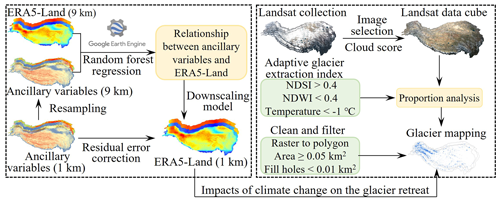
Figure 3 presents a flowchart that outlines the process for analyzing the impacts of climate change on glacier retreats on the Tibetan Plateau. To evaluate the potential effects of the downscaled meteorological factors on changes in glacier extent, a linear regression model has been employed. This model analyzes the relationships between annual and seasonal meteorological factors and the changes in glacier area within these subzones. This method is a straightforward approach for predicting a quantitative glacier area response (Y) on the basis of a single meteorological variable (X). It assumes that there is a linear relationship between X and Y. Mathematically, the linear relationship was estimated as follows:

$$\begin{array}{}\text{(9)}& Y=a+bX,\end{array}$$

where a and b are two constants that represent the intercept and slope terms in the linear model, and these two terms are determined by fitting the changes in glacier extent to the meteorological factors, which include both annual and seasonal air temperature and precipitation, over the period from 1990 to 2020 in each subzone. In this study, the impacts of annual and seasonal temperature and precipitation on the changes in glacier extent are included in one regression model, and the interactions between air temperature and precipitation are not accounted for in this analysis.

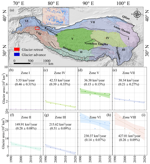
Figure 4 Spatial changes in glacier extent throughout the observation period in subzones of the Tibetan Plateau. (a) Spatial distributions of glacier area changes on the Tibetan Plateau. (b–i) Time series of glacial area change rates in zones I, IV, V, VII, II, III, VI, and VIII, respectively; the dot indicates the glacier area in each observation period, the line indicates the linear fitting of the time series of glacier change, and the shading represents the 90 % confidence band.

Figure 5 Comparison results of glacier mapping in 2000, 2005, and 2010 and the reference RGI 6.0 and RGI 7.0 debris-free glaciers.

4 Results

4.1 Time series' glacier-mapping results

The debris-free glacier area on the Tibetan Plateau exhibited a decline from 94.95 × 10³ km² in 1990 to 61.16 × 10³ km² by 2020, corresponding to an average retreat rate of 1.08 ± 0.28 × 10³ km² yr⁻¹. Figure 4 illustrates the spatial changes in glacier extent throughout the observation period. The observed changes in glacier extent on the Tibetan Plateau are relatively minor in its interior and intensify towards the periphery. Notably, the most pronounced retreat occurs at the edges, especially in zones I and III, situated in the eastern and southeastern regions of the plateau, respectively. Conversely, glacier advance is predominantly seen in the Karakoram area, a phenomenon referred to as the Karakoram anomaly (Fig. 4a). Additionally, a minor advancement of glaciers is also noted in the transitional area between zones II and VIII. Figure 4 reveals marked variations in glacier area change rates across different subzones, despite a general shrinkage trend. During the observation period, the rate of changes in glacier extent varied from 0.14 ± 0.07 % yr⁻¹ in Zone VI to 0.51 ± 0.09 % yr⁻¹ in Zone III. Notably, a rapid retreat occurred in 2000, particularly in zones II, V, VI, and VIII. From 2000, there was a slight increase in glacier areas in zones II, V, and VII. Since 2010, these subzones have exhibited either a stable or a marginally decreasing glacier area, suggesting a relatively stable glacial state. It can also be observed that there is an increase in glacier area in zones II and V between 2000 and 2005 (Figs. 4 and 5); some studies have shown that there is a slight increase in glacier area in the eastern Kunlun, inner Tibet, and central Himalayan regions from 2000 to 2005 (Huang et al., 2021), these areas correspond to zones II and V. In addition, there was also a notable increase in glacier area between 2005 and 2010 in zones VI and VIII, which corresponds to the increased glacier area in the Karakoram Range from 2006 to 2010 (Yao et al., 2012).

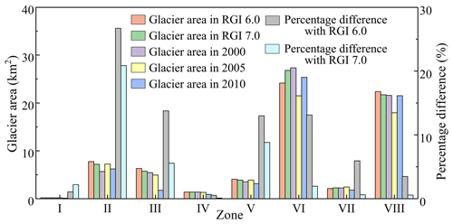
A comparative analysis of glacier mapping in 2000, 2005, and 2010 against the reference RGI 6.0 and RGI 7.0 debris-free glaciers in these subzones is presented in Fig. 5. The mapped glaciers in these areas generally align with the debris-free glaciers delineated in RGI 6.0 and RGI 7.0, particularly in zones I, IV, V, and VII. These subzones, located primarily in the interior of the Tibetan Plateau, feature a comparatively smaller glacier area relative to other subzones. Given that the target year in RGI 6.0 and RGI 7.0 was 2000 (RGI 7.0 Consortium, 2023), the glacier area in 2000 was utilized for comparison (to facilitate a more intuitive comparison of differences), with the percentage difference between the 2000 glacier and the reference RGI 6.0 and RGI 7.0 glacier detailed in Fig. 5. This analysis reveals that the percentage differences between the mapped 2000 glacier area in this study and those from RGI 6.0 and RGI 7.0 are relatively small, especially for the reference RGI 7.0 glacier data, mainly because 35 % of all RGI 6.0 outlines were dated to 5 or more years away from the target year 2000, while this number is down to 23 % in RGI 7.0 (RGI 7.0 Consortium, 2023).

Table 2 Quantitative comparison results of glacier mapping in 2000, 2005, and 2010 and the reference RGI 6.0 and RGI 7.0 debris-free glaciers.

To quantitatively evaluate the glacier-mapping results, the correctness, completeness, and F1-score metrics are applied to the mapped glaciers and the reference RGI 6.0 and RGI 7.0 debris-free glaciers. Table 2 demonstrates that the correctness of the glaciers mapped during these three periods consistently exceeds 0.7, affirming the accuracy of the mapping results. In addition, the glaciers mapped in 2000 display greater consistency compared with those mapped in 2005 and 2010, which is in agreement with the results depicted in Fig. 5. Note that the accuracy of our mapped glaciers in 2000 using the latest RGI 7.0 glacier data is higher than that using the RGI 6.0 glacier data, which further confirms the accuracy of our mapped glaciers; in addition, the target year of RGI 6.0 and RGI 7.0 glacier data is 2000. Thus, the completeness of the mapped glaciers in this study was particularly poor in 2010.

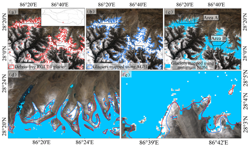
Figure 6 Comparisons between the glaciers delineated using the AGEI method and the corresponding minimum NDSI values for (a) the debris-free RGI 7.0 glacier, (b) glaciers mapped using the AGEI method, and (c) glaciers mapped using the minimum NDSI. (d) Comparison results of glacier mapping in Area A. (e) Comparison results of glacier mapping in Area B. The base map is Landsat 8 mosaic images obtained from 2018 to 2022 in the ablation season.

Huang et al. (2021) utilized the minimum NDSI value in each pixel for glacier mapping, which proved to be particularly effective with respect to minimizing the influence of seasonal snow cover. In this study, the minimum NDSI method is also adopted to verify the glacier-mapping results. Figure 6 illustrates a comparison between the glaciers delineated using the AGEI method and the corresponding minimum NDSI values in 2020. The base map is Landsat 8 mosaic images obtained from 2018 to 2022 in the ablation season. It can be seen that the glacier-mapping errors caused by glacial lakes can be minimized using the AGEI method compared with the minimum NDSI method, as depicted in Fig. 6d. Area B may be affected by thin clouds during a certain period, making the NDSI value at that time less than 0.4, but the glaciers in this area can be better identified by the AGEI method (see Fig. 6e). For the whole Tibetan Plateau, the correctness of the mapped glaciers using the AGEI method is 0.76 for the period of 2000 (see Table 2), while the correctness is 0.72 when using the NDSI method.

The minimum NDSI method has limitations with respect to its robustness, especially when encountering image noise, such as small icebergs, brash ice, and haze, or other issues, like Scan Line Corrector failure in Landsat 7 images (Chander et al., 2009; Shugar et al., 2020). Additionally, the cloud score threshold of 60 might have included glacier pixels under thin clouds, potentially leading to NDSI values below 0.4 and affecting glacier delineation accuracy. To mitigate noise and omissions in glacier mapping, the AGEI method is proposed; this method entails using proportions of the Landsat data cube that meet the predefined NDSI, NDWI, and surface temperature criteria, calibrated through visual comparisons with contemporary optical image mosaics. Furthermore, the AGEI method incorporates surface temperature, a crucial factor when dealing with glacial polygons adjacent to glacial lakes (Shugar et al., 2020). This consideration is vital because glacial lakes, being warmer than the surrounding glaciers and ice, may not be wholly excluded by the NDWI threshold alone.

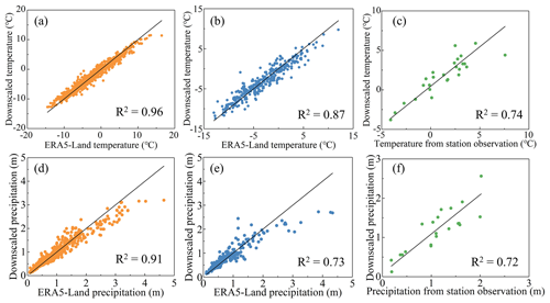
Figure 7 Comparisons between the downscaled meteorological products and the training samples, validation samples, and station observations: (a–c) comparative results of the downscaled air temperature with the training samples, validation samples, and station observations, respectively; (d–f) comparative results of the downscaled precipitation with the training samples, validation samples, and station observations, respectively.

4.2 Downscaled results of the ERA5-Land reanalysis datasets

The ERA5-Land reanalysis datasets, specifically the 2 m air temperature and total precipitation, have been downscaled using the random forest method over the observation period (i.e., from 1988 to 2022). Prior to conducting trend analysis on these downscaled meteorological products, their accuracy is initially evaluated against observational data from meteorological stations. The locations of these meteorological stations are shown in Fig. 1; the distribution of the training and validation samples are shown in Fig. S2 in the Supplement, and the number of respective training and validation samples are 4000 and 1000 for the downscaling analysis. Figure 7 illustrates the comparison between the downscaled meteorological products and the training samples, validation samples, and station observations. The consistency of the downscaled products with these datasets is evident, as reflected by the high R² values. Therefore, the downscaled meteorological products are deemed suitable for use in subsequent analyses.

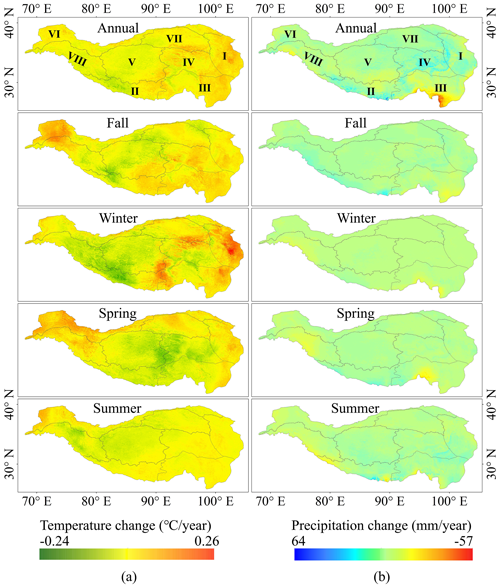
Figure 8 Trend analysis results of the downscaled meteorological datasets for (a) 2 m air temperature and (b) precipitation.

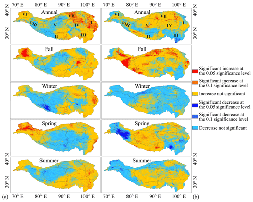
Figure 9 Significance of the trend analysis results for (a) 2 m air temperature and (b) precipitation. Note that the legend on the right-hand side is universal for both the air temperature and precipitation.

Figure 8a presents the overall upward trend in the 2 m air temperature during the observation period, with the highest increase observed in winter at a rate of 0.26 °C yr⁻¹, specifically in the eastern Tibetan Plateau (Zone I). However, this warming trend varies across different seasons. Across the Tibetan Plateau, the observed rates of seasonal temperature increase are as follows: an annual increase of 0.14 °C per decade, an autumn increase of 0.16 °C per decade, a winter increase of 0.04 °C per decade, a spring increase of 0.008 °C per decade, and a summer increase of 0.04 °C per decade. Additionally, the rate of increase in the 2 m air temperature displays significant spatial heterogeneity. For instance, the areas experiencing the most rapid warming are predominantly located in the eastern and southeastern parts of the Tibetan Plateau, specifically in zones I, III, and IV, with this trend being particularly pronounced during the autumn and winter seasons. Notably, these regions of accelerated warming align with the zones of fastest glacier retreat, as depicted in Fig. 4. Figure 9a illustrates the significance of both annual and seasonal changes in air temperature. It reveals that the regions with significant temperature increases are mainly in the eastern part of the Tibetan Plateau. In contrast, the southwestern and central areas, specifically zones V and VIII, display a marked decreasing trend in temperature. Correspondingly, as shown in Fig. 4, the glacier retreat rates in these two zones are relatively low. Interestingly, in the transitional area between zones II and VIII, there is a notable decreasing trend in air temperature during the winter season, which aligns with the area increase in some individual glaciers in this region (see Fig. 4a).

In contrast to the 2 m air temperature changes, the total precipitation across the Tibetan Plateau does not exhibit a consistent increasing or decreasing trend, as illustrated in Fig. 8b. The highest increase in precipitation rate, reaching up to 64 mm yr⁻¹, is observed on the southern part of the plateau, specifically in Zone II. On the other hand, the most significant decrease in precipitation is noted in the southeastern region, identified as Zone III. The average rates of precipitation change vary by season. They were 3.5 mm per decade annually, 7.0 mm per decade in autumn, −5.0 mm per decade in winter, −1.5 mm per decade in spring, and 1.2 mm per decade in summer. Like the 2 m air temperature change, the precipitation variation across the region also demonstrates significant spatial heterogeneity. For instance, the area of some individual glaciers increased in the southwestern Himalayas and the Karakoram Range, which may have been caused by a marginal increase in precipitation during the observation period. Furthermore, the southeastern Tibetan Plateau, identified as Zone III, exhibits a notable decreasing trend in annual precipitation, which aligns with the observed decrease in glacier extent in this zone. Additionally, Fig. 9b highlights that the annual precipitation markedly increases in the transitional area between zones II and VIII, whereas it significantly decreases on the southeastern Tibetan Plateau.

Figure 10 Impacts of meteorological factors on the changes in the glacier extent for (a) 2 m air temperature and (b) precipitation.

4.3 Impacts of climate change on the glacier retreat

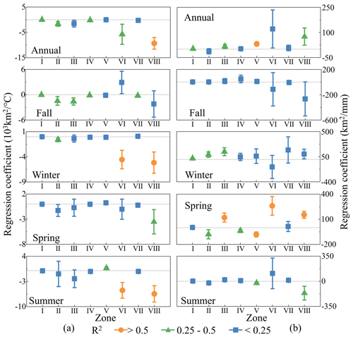
The effects of the downscaled meteorological factors on changes in glacier extent are presented in Fig. 10. Figure 10a illustrates the impact of the downscaled 2 m air temperature on changes in glacier area. Across all of the subzones, the glacier area may decrease with annual temperature increases, and the most pronounced impacts can be observed in Zone VIII, with a value of −9.34 × 10³ km² °C⁻¹. When considering seasonal variations, the impact of temperature changes on glacier retreat is especially notable in zones VI and VIII for the winter and summer seasons. The effects of winter air temperatures on glacier change can be −4.56 × 10³ km² °C⁻¹ and −5.16 × 10³ km² °C⁻¹ in zones VI and VIII, respectively, and the corresponding values for summer air temperature reach −5.49 × 10³ km² °C⁻¹ and −6.46 × 10³ km² °C⁻¹ (Table S1 in the Supplement). However, the impact of spring temperature on glacier area change is less evident except for Zone VIII.

Figure 10b presents the effects of downscaled precipitation on changes in glacier extent. It reveals that an increase in annual precipitation can help mitigate glacier retreat except for Zone II. However, this restraining impact of annual precipitation is evident only in zones III, V, and VIII, with values of 16, 32, and 75 km² mm⁻¹, respectively (Table S2 in the Supplement). Note that, although the correlation coefficient of the annual precipitation on changes in glacier extent in Zone VI is 121 km² mm⁻¹, the R² is only 0.19. Thus, this restraining impact of annual precipitation on the glacier retreat is not evident in Zone VI. When considering seasonal variations, the most restraining impact can be observed in Zone VI for the spring season, with a value of 261 km² mm⁻¹ (R² = 0.52). However, the effects of autumn precipitation on glacier change in all subzones are not apparent. In addition, for Zone VIII, the increases in winter and spring precipitation amounts are found to counteract glacier retreat, while increased precipitation in summer might actually accelerate it. This observed phenomenon could be attributed to the different forms of precipitation. In this study, the total precipitation amount encompasses both rainfall and snowfall, but these two forms have distinct impacts on changes in glacier extent (Su et al., 2022). Snowfall is beneficial for glacier formation and growth, as it increases surface albedo and contributes to mass accumulation on the glaciers. On the other hand, rainfall tends to accelerate glacier retreat due to its influence on the surface energy budget. For instance, rainfall can reduce surface albedo and release latent heat, both of which are factors that contribute to the melting of glaciers.

5 Discussion

5.1 Discussion on the spatial variability in glacier retreat

The distinct regional variations in changes in glacier extent, with the most pronounced retreat observed in the Himalayas and on the southeastern Tibetan Plateau (i.e., zones II and III), are shown in Fig. 4. Numerous studies corroborate that the retreat in the Himalayan region is marked by the most substantial reductions in glacier length and area as well as by the most negative glacier mass balance (Yao et al., 2012; Latif et al., 2019; Zhang et al., 2021). The rising temperatures and declining precipitation on the southeastern Tibetan Plateau (i.e., Zone III), as depicted in Fig. 9, are likely contributing factors to the glacier retreat observed in this region. Moreover, a gradient of glacier shrinkage is observed, diminishing progressively from the Himalayas towards the continental interior (i.e., from Zone II to Zone V), indicating a less pronounced retreat in these regions. This area is characterized by the least glacier retreat, minimal area reduction, and a more positive mass balance (see Fig. 4; Yao et al., 2012). This study examines the effects of downscaled air temperature and precipitation on glacier retreat across various subzones. However, it does not account for the interactions between air temperature and precipitation. In fact, glaciers are sensitive to the rising air temperature and precipitation that occurs at temperatures near 0 °C. Such conditions are significant contributors to the loss of snow and ice cover, most notably during the spring season (Kang et al., 2009; Bibi et al., 2018). Therefore, consideration of the interaction between air temperature and precipitation is essential for a more comprehensive analysis of glacier retreat under climate change. Moreover, atmospheric circulation patterns play a crucial role in dictating the spatial variability in the air temperature and precipitation changes, leading to diverse impacts of climate change on glacier retreat across different regions. The subzone divisions illustrated in Fig. 1 incorporate these variations in atmospheric circulation processes. As a result, analyzing glacier changes within these distinct subzones offers a more nuanced and reasonable approach to understanding the effects of climate change on glacier retreat.

Figure 11 Comparison of the mean and median glacier debris thickness against the glacier retreat rate in various subzones.

5.2 Discussion on the influence of debris thickness on glacier retreat

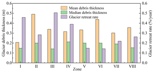
Using the glacier boundaries of RGI, it was estimated that 10 % of glaciers are covered by debris on the Tibetan Plateau and its surrounding areas (Scherler et al., 2018a), and the debris-covered glaciers in this region are mainly distributed in the Himalayas (Ojha et al., 2017). The debris layer makes the melting process of glaciers complicated, and debris-covered glaciers have contrasting melting mechanisms and climate response patterns compared with debris-free glaciers (Chen et al., 2023). In this study, changes in glacier extent only refer to changes in debris-free glaciers. This study has shown that the retreat of debris-free glaciers, as reflected by changes in glacier area, is primarily due to climate warming. However, as depicted in Fig. 10, the impacts of climate change on glacier retreat show significant spatial heterogeneity. This variability is primarily attributed to the complex interplay of climatic, geographic, and topographic factors. Among these factors, elements like debris cover, ice cliffs, and glacial lakes play crucial roles in determining glacier responses to climatic shifts (Johnson and Rupper, 2020; Su et al., 2022; Chen et al., 2023). Notably, the thickness of supraglacial debris is a crucial factor that can significantly influence the rate of glacier retreat in the context of climate change (Pratap et al., 2015). To explore the potential impacts of supraglacial debris thickness on glacier retreat, debris thickness datasets are obtained from Rounce et al. (2021). Figure 11 presents a comparison of the mean and median glacier debris thickness against the glacier retreat rate in various subzones. The analysis reveals that areas experiencing rapid glacier retreat, such as zones I and III, are characterized by lower mean and median values of debris thickness. This observation aligns with research suggesting that thinner debris layers on glaciers lead to increased absorption of solar radiation, thereby accelerating the melting of the glacier and hastening its retreat (Rounce et al., 2018; Chen et al., 2023). Conversely, in areas with thicker debris layers, such as zones V and VI, the thermal insulation provided by the debris predominates, thereby slowing down the glacier retreat. However, this analysis focuses only on different subzones, which might yield results that deviate from studies conducted on individual glaciers. Despite this, considering the response of glacier retreat to debris thickness remains a valuable aspect for further exploration, especially in the context of analyzing the retreat of a single glacier under the influence of climate change.

Figure 12 Glacier area change (%) by the end of the century for the three Shared Socioeconomic Pathways (SSPs) in various subzones.

5.3 Discussion on the implications of the future climate projections on changes in glacier extent

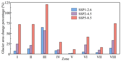
Projections of future climate change play a fundamental role in improving understanding of the climate system as well as characterizing future changes in glacier extent and mass balance (Rounce et al., 2023). In this study, the latest Coupled Model Intercomparison Project Phase 6 (CMIP6) dataset was adopted to project changes in annual temperature and precipitation by the end of the century (i.e., the year 2100). Three Shared Socioeconomic Pathways (SSPs) were collected for temperature and precipitation analyses: the low-forcing scenario SSP1-2.6, the medium-forcing scenario SSP2-4.5, and the high-forcing scenario SSP5-8.5. According to these scenarios, for the whole Tibetan Plateau, the temperature would rise 1.03 °C (SSP1-2.6), 1.95 °C (SSP2-4.5), and 4.72 °C (SSP5-8.5), while the change in precipitation would be −45 mm (SSP1-2.6), 5 mm (SSP2-4.5), and 89 mm (SSP5-8.5) by the end of the century compared with the year 2020. Based on the linear regression between the meteorological factors and changes in glacier extent shown in Fig. 10, it was anticipated that the glacier area would be reduced by 10.92 % (SSP1-2.6), 25.44 % (SSP2-4.5), and 55.42 % (SSP5-8.5) for the whole Tibetan Plateau. Figure 12 presents the glacier area change (as a percentage) in 2100 for the three SSPs in various subzones. It can be seen that the glacier area is projected to decrease significantly across all subzones under the high-forcing scenario SSP5-8.5, with debris-free glaciers in Zone III expected to disappear by the end of the century, reflecting the highest glacier retreat rate shown in Fig. 4g. The retreat of glaciers could lead to unsustainable water supplies in major rivers and increase geohazards, such as glacier lake expansion and outburst flooding, which might threaten the livelihoods of downstream regions. For example, glacier melt on the southeastern Tibetan Plateau (i.e., Zone III) would enhance the duration and intensity of extreme floods, which would also amplify the effects of future flooding on socioeconomics (Sun et al., 2024).

6 Conclusions

This study proposed an adaptive glacier extraction index (AGEI) method to map glacier time series on the Tibetan Plateau, analyzing glacier retreat with downscaled air temperature and precipitation from 1988 to 2022. The following conclusions are reached based on the results presented:

1. Utilizing the Google Earth Engine platform and Landsat archives, this study maps the glaciers of the Tibetan Plateau at 5-year intervals from 1988 to 2022 using the AGEI method. The total debris-free glacier area decreased from 94.59 × 10³ to 61.16 × 10³ km², with an average annual retreat rate of 1.08 ± 0.28 × 10³ km². The rates of glacier retreat varied significantly across the eight subzones, ranging from 0.14 ± 0.07 % to 0.51 ± 0.09 % yr⁻¹ over the observation period.

2. The ERA5-Land reanalysis datasets have been downscaled for this study to examine annual and seasonal trends from 1988 to 2022. There is an overall increase in the 2 m air temperature during this period, with the maximum rate of increase reaching 0.26 °C yr⁻¹, particularly in the winter season. The fastest-warming areas are predominantly in the eastern and southeastern parts of the Tibetan Plateau. A slight increase in precipitation is mainly observed in the southwestern Himalayas and the Karakoram Range, which may have helped mitigate reductions in the glacier area in these regions.

3. There is a negative correlation between changes in glacier extent and annual temperature variations, and the most pronounced impacts are observed in Zone VIII, with a value of −9.34 × 10³ km² °C⁻¹. The impact of winter and summer temperature changes on glacier retreat is especially notable in zones VI and VIII. The increase in annual precipitation can help mitigate glacier retreat except for Zone II, and the most restraining impact is observed in Zone VI for the spring season, with a value of 261 km² mm⁻¹. For Zone VIII, the increases in winter and spring precipitation amounts are found to counteract glacier retreat, while increased precipitation in summer might actually accelerate it.