Evaluation of satellite methods for estimating supraglacial lake depth in southwest Greenland

Supraglacial lakes form on the Greenland ice sheet in the melt season (May to October) when meltwater collects in surface depressions on the ice. Supraglacial lakes can act as a control on ice dynamics since, given a large enough volume of water and a favourable stress regime, hydrofracture of the lake can occur, which enables water transfer from the ice surface to the bedrock, where it can lubricate the base. The depth (and thus volume) of these lakes is typically estimated by applying a radiative transfer equation (RTE) to optical satellite imagery. This method can be used at scale across entire ice sheets but is poorly validated due to a paucity of in situ depth data. Here we intercompare supraglacial lake depth detection by means of ArcticDEM digital elevation models, ICESat-2 photon refraction, and the RTE applied to Sentinel-2 images across five lakes in southwest Greenland. We found good agreement between the ArcticDEM and ICESat-2 approaches (Pearson's r=0.98) but found that the RTE overestimates lake depth by up to 153 % using the green band (543–578 nm) and underestimates lake depth by up to 63 % using the red band (650–680 nm). Parametric uncertainty in the RTE estimates is substantial and is dominated by uncertainty in estimates of reflectance at the lakebed, which are derived empirically. Uncertainty in lake depth estimates translates into a poor understanding of total lake volume, which could mean that hydrofracture likelihood is poorly constrained, in turn affecting ice velocity predictions. Further laboratory studies to constrain spectral radiance loss in the water column and investigation of the potential effects of cryoconite on lakebed reflectance could improve the RTE in its current format. However, we also suggest that future work should explore multi-sensor approaches to deriving lake depth from optical satellite imagery, which may improve depth estimates and will certainly result in better-constrained uncertainties.

1 Introduction

Supraglacial lakes form when meltwater collects in surface depressions on glaciers and ice sheets. On the Greenland ice sheet, lakes form in approximately the same locations each melt season from May to October (Sundal et al., 2009) as their positions are controlled by bedrock topography (Echelmeyer et al., 1991; Krawczynski et al., 2009). Alongside rivers and streams, supraglacial lakes form a complex hydrological system of water storage and transport on the ice sheet surface. As the melt season progresses, supraglacial lakes grow in size through the accumulation of meltwater. These lakes either drain or refreeze, with ∼ 34 % of lakes at lower elevations draining slowly, ∼ 14 % draining rapidly, and ∼ 50 % refreezing. At higher elevations, lakes tend to refreeze (Selmes et al., 2013). Drainage can occur slowly over the ice surface through supraglacial channels or rapidly through the ice if the weight of the water is sufficient to drive a crevasse through the full ice thickness to the bed. This process is known as hydrofracture, and related drainage events can occur in as little as 2 h (Das et al., 2008). In these events, the water is routed to the base of the ice sheet, where it can cause a hydraulic pressure increase that temporarily lifts the ice off the bed. This process can enhance basal sliding and increase ice flow rates (Fitzpatrick et al., 2013; Tedesco et al., 2013; Christoffersen et al., 2018; Tuckett et al., 2019; Maier et al., 2023). Short-term increases in meltwater input cause temporary spikes in water pressure, leading to ice acceleration. However, an increase in mean melt supply does not necessarily cause an increase in ice sheet velocity (Schoof, 2010). Ergo, knowing the volume of water held on the ice sheet at any one time – and thus the potential for temporary spikes in water pressure through hydrofracture – is important for modelling ice sheet dynamics.

Our understanding of ice sheet behaviour assumes that we have an understanding of meltwater delivery (Zwally et al., 2002; Parizek and Alley, 2004). If the calculated depth of supraglacial lakes is inaccurate, the volume of the lake is inaccurate, thus meaning our calculations of injected meltwater to the ice sheet bed are also inaccurate. As a result, under- or overestimating the volume of meltwater holds consequences for the models on which we base our understanding of ice dynamics (e.g. Tedesco et al., 2013; Christoffersen et al., 2018).

To understand the amount and rate of meltwater delivery to the ice sheet bed, we require spatially and temporally continuous observations of lake volume. Our study area, located in the southwest Greenland ice sheet (Fig. 1), includes the lower Watson River basin (5800 km²). This basin has a meltwater coverage (including supraglacial lakes, streams, and rivers) of 250 km² (Emily Glen, personal communication, 22 July 2022), meaning it is not feasible to acquire spatially and temporally continuous lake volume data from field surveys. Instead, several satellite-based methods can be used to estimate supraglacial lake depths remotely, potentially providing high spatial and temporal coverage. These methods are as follows: physics-based modelling, such as the application of the radiative transfer equation (RTE) proposed by Philpot (1987) to optical satellite imagery (Moussavi et al., 2020); laser altimetry, which is used to measure lake depths directly from photon refraction (Fair et al., 2020); the use of digital elevation models to ascertain lake depth from the underlying ice surface topography (Yang et al., 2019); and empirical models derived from regression of in situ depth measurements with remotely sensed data (Pope et al., 2016).

These methods each have known advantages and limitations for deriving lake depths. Physics-based models applied to optical satellite data (e.g. Sentinel-2) provide continuous spatial coverage at high-resolution temporal sampling (i.e. every 5 d), and they can be used at scale. ICESat-2 can directly measure lake depths but is limited to 1-D profiles along discrete satellite tracks which are spatially distant (4.1 km between acquisition beams of neighbouring satellite tracks at 67^∘ N) and have coarse temporal sampling, inhibiting an assessment of lake dynamics as supraglacial hydrology evolves on sub-daily timescales (Das et al., 2008). ArcticDEM data is even more sporadic in space and time, with periods of months between acquisitions and missing data caused by cloud cover. However, ArcticDEM offers a spatial resolution (2 m) of 1 order of magnitude higher than Sentinel-2 and thus enables a more detailed assessment of lake bathymetry – for example, to assess whether a lake basin contains open or healed crevasses that may promote lake drainage by hydrofracture. Although empirical models derived through the regression of in situ depth measurements with remotely sensed data have been shown to define reasonable lake depth (Pope et al., 2016), their coefficients are spatially constrained to the area in which the original in situ measurements were taken and are, therefore, unreasonable to apply on the ice sheet scale. Intercomparing multiple depth detection methods increases our confidence in the depths calculated at locations where there is agreement between methods. This is especially important in the absence of ground truth data. Here, we examine and intercompare the performance of three satellite-based methods – a physics-based model that uses a radiative transfer equation (RTE), ICESat-2 laser altimetry, and ArcticDEM digital elevation models – in determining the depth of a test dataset of supraglacial lakes in the southwest Greenland ice sheet, where Greenlandic supraglacial lakes are extensive and numerous (Hu et al., 2022).

2 Data and methods

2.1 Study region and supraglacial lakes

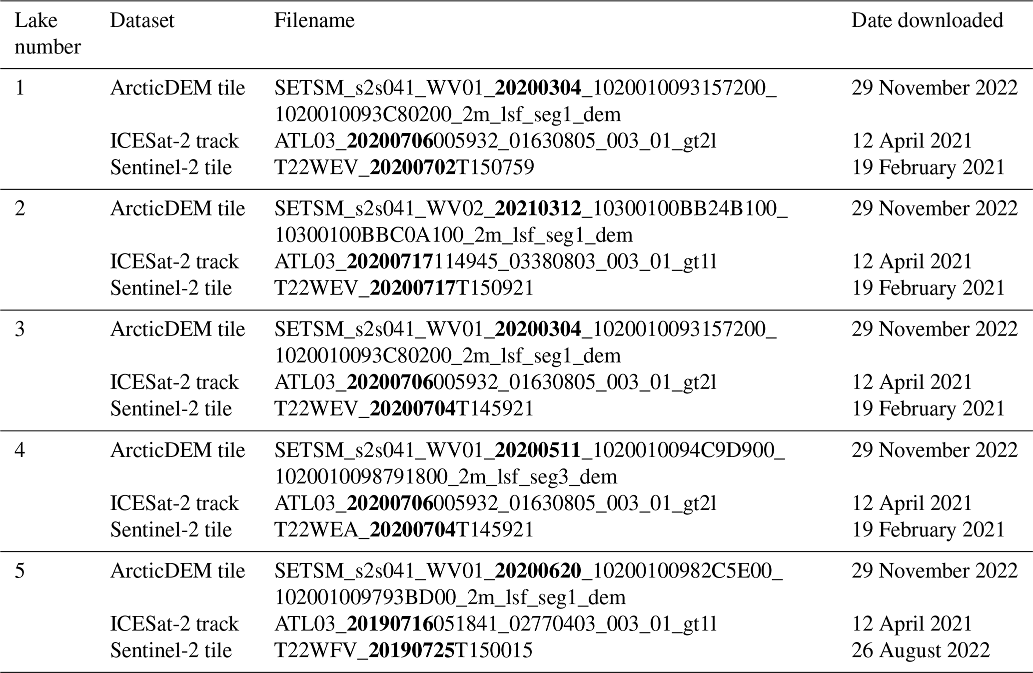
Our study region (Fig. 1) is located in western Greenland and contains part of the Watson River basin, known for abundant supraglacial lake coverage. This region contains both active (repeatedly filling and draining) and non-active lakes and is known to respond dynamically to hydrological perturbations (e.g. Das et al., 2008; Chudley et al., 2019). Five lakes in this region were found to be suitable for depth retrieval from all three of the datasets (with the availability of ICESat-2 data being the main limitation; see Appendix A1). Each of the five supraglacial lakes are active, are crossed by an ICESat-2 reference ground track, and have both concurrent optical imagery and a corresponding digital elevation model (DEM) showing an empty lake basin. These five lakes span a range of sizes (0.8–3.1 km²) and appear at a range of elevations (1150–1500 m a.s.l.), as shown in Fig. 1.

We apply three different methods to measure the depth of each of our five lakes. These methods are described in detail below.

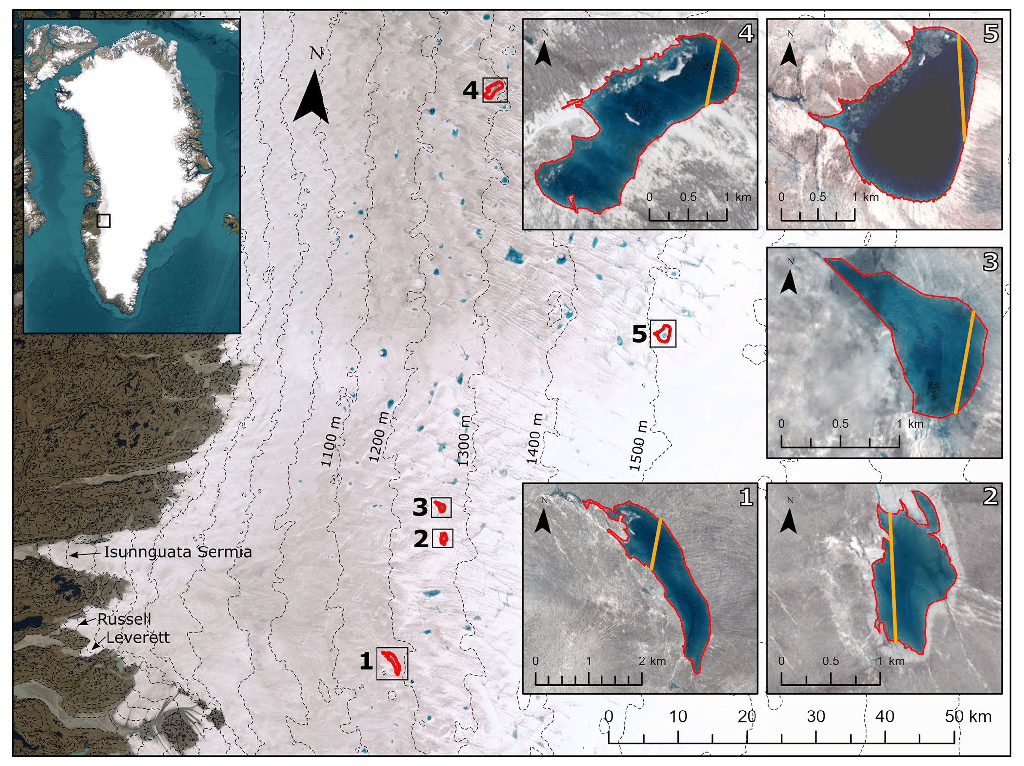
Figure 1 The locations of the five supraglacial lakes in relation to the study region. Contour lines calculated from the ArcticDEM 100 m mosaic are visible on the base map as dashed grey lines. The inset map indicates the location of the study area within Greenland. Panels (1)–(5) show Lake 1 to Lake 5 in detail, where the background is a true-colour image acquired on the date shown in Table A1 for each lake. The manually delineated lake outline is given in red, and the ICESat-2 transect is given in orange. The ICESat-2 ground tracks were cropped to the lake edges. The background images in panels (1)–(5) are the Sentinel-2 tiles detailed in Table A1. The base map data are courtesy of Earthstar Geographics via Esri.

2.2 Method 1: radiative transfer equation applied to optical satellite imagery

Here, we apply the RTE (Eq. 1) first presented in Philpot (1987) to both red (0.65–0.68 µm) and green (0.54–0.58 µm) bands of level-1C Sentinel-2 optical satellite imageries which are temporally (±10 d) concurrent with the ICESat-2 data for each of our five case study lakes (Table A1 in the Appendix). To confirm that the lakes had not changed in size between the ICESat-2 and Sentinel-2 acquisition dates, we undertook a visual appraisal of optical satellite imagery acquired approximately 15 d either side of the ICESat-2 acquisition date. Sentinel-2 has a spatial resolution of 10 m and a revisit period in this region of about 5 d (Drusch et al., 2012). The RTE method is commonly applied to optical satellite data in order to determine lake depth on the Greenland ice sheet (e.g. Williamson et al., 2018; Moussavi et al., 2020; Datta and Wouters, 2021). We chose to use Sentinel-2 level-1C products which are pre-packaged as orthorectified, map-projected imageries of scaled top-of-atmosphere data, in keeping with these previous studies. We converted these values to unscaled top-of-atmosphere reflectance using standard methods (Williamson et al., 2018; Moussavi et al., 2020; Datta and Wouters, 2021). Although previous studies have averaged the depths retrieved from the red-band RTE and the panchromatic band of Landsat 8 (Pope et al., 2016; Williamson et al., 2018), we do not do so within this study as Sentinel-2 does not have a panchromatic band. Additionally, this study specifically aims to understand the uncertainties associated with applying the physically based RTE to data acquired at a single band, and so an empirical averaging without a clear physical justification does not serve the purposes of this research.

The radiative transfer approach to modelling lake depth is based on the assumptions of the Bouguer–Lambert–Beer law. Equation (1) gives the formulation of the equation presented by Philpot (1987), written in terms of reflectance and inverted into the logarithmic form:

$$\begin{array}{}\text{(1)}& z={\displaystyle \frac{\ln \left(A_d-R_{\mathrm{\infty }}\right)-\ln \left(R_w-R_{\mathrm{\infty }}\right)}{g}},\end{array}$$

where A_d represents the lake bottom albedo or reflectance, R_∞ indicates the reflectance of optically deep water, R_w is the recorded reflectance of a given pixel, g is the coefficient for spectral radiance loss in the water column, and z represents lake depth in metres. A_d, R_∞, and g can each take a range of plausible values, and so here we consider them to be tuneable parameters.

Here we take A_d to be the average reflectance value in a 30 m wide ring (three pixels in Sentinel-2, after Moussavi et al., 2020) around each of the five lakes to provide a unique A_d value for each lake. This is the same way that A_d is estimated in previous studies. R_∞ represents reflection from the water column and is commonly taken as the reflectance of optically deep, clear, and still water, i.e. where it is reasonable to assume that there is no bed reflectance or sediment contamination (Sneed and Hamilton, 2007). Ideally, this would be done using ocean water pixels in the same satellite image from which lake depth is acquired. However, here we find that no ocean water was visible in the images we used, and so we substituted the image acquired closest in time and space in which ocean water was visible (Appendix A2). To estimate R_∞, we averaged the reflectance of the 10 darkest pixels in each substitute image after manually filtering out pixels obviously associated with sediment traces or sensor-related scanning issues. This is slightly different to the way that R_∞ has been calculated in previous studies but does not produce values that are appreciably different.

We calculate g using Eq. (2), which accounts for the scattering of both downwelling (K_d) and upwelling (K_u) light:

$$\begin{array}{}\text{(2)}& g=K_{\mathrm{d}}+K_{\mathrm{u}}.\end{array}$$

K_d is calculated using Eq. (3) and is wavelength specific:

$$\begin{array}{}\text{(3)}& K_{\mathrm{d}}=a_{\mathrm{w}}+{\displaystyle \frac{\mathrm{1}}{\mathrm{2}}}{b}_{\mathrm{m}}^{\mathrm{fw}},\end{array}$$

where a_w is the absorption coefficient for pure water, and $b_{\mathrm{m}}^{\mathrm{fw}}$ is the backscattering coefficient for molecular scattering in freshwater. These are laboratory-derived values and are taken from Smith and Baker (1981). Very few laboratory estimates exist of K_u (Philpot, 1989), and so previous studies have typically taken K_u to be equal to K_d (e.g. Maritorena et al., 1994; Sneed and Hamilton, 2007). We argue, however, that K_u must be larger than K_d because upwelling photons are more rapidly attenuated than downwelling photons in water (Kirk, 1989). In fact, experimental studies suggest that K_u could be as high as 2.5K_d (Kirk, 1989). Here, we use an average of these two values and take K_u to be 1.75 K_d. This will naturally lead to a higher value of g than commonly used in supraglacial lake depth studies, and we note that it has been recently suggested that this would lead to more accurate lake depths (Brodský et al., 2022).

We estimate uncertainty by first assigning a range of plausible values to each tuneable parameter (Appendix A3) and then applying the RTE to every permutation of the combination of these values. The standard deviation of depths calculated using these permutations was taken to represent the uncertainty of the depth measurement.

We find it helpful to compare our estimates to those given using previously published methods of estimating our tuneable parameters. We calculate these literature values of the parameters as follows: g=2K_d (Sneed and Hamilton, 2007), where K_d is as described in Eq. (3), and R_∞ is the reflectance of the single darkest pixel in the deep-sea scene (e.g. Georgiou et al., 2009; Pope et al., 2016).

In our modelling we assume the lake substrate is homogenous, suspended or dissolved particles are minimal, there is no inelastic scattering or fluorescence, the effects of wind are minimal, and lake bottom pixels are parallel to the lake surface, following Sneed and Hamilton (2011).

We do not average band-specific depth estimates here for the reasons outlined previously; however, we do note that this has been done in previous studies (e.g. Pope et al., 2016; Williamson et al., 2018).

2.3 Method 2: ArcticDEM

ArcticDEM is an open-access collection of high-resolution DEMs produced by the Polar Geospatial Center (Porter et al., 2022). The dataset is assembled from individual stereoscopic DEMs that are derived from pairs of high-resolution optical imagery acquired by the WorldView-1, WorldView-2, WorldView-3, and GeoEye-1 satellites (Morin et al., 2016). The DEMs are generated by applying the Surface Extraction from TIN-based Searchspace Minimization (SETSM) software to stereoscopic image pairs (Noh and Howat, 2017). Here, we use the most recent version of ArcticDEM data (version s2s041, release 8). The tile reference numbers of the DEMs used in this study are detailed in Table A1; all available ArcticDEM DEMs of the study region were acquired from the Polar Geospatial Center.

In ArcticDEM, full lakes are represented by flat surfaces. To measure their depth, we need to examine the shape of the basin before it has filled or after it has drained. As drained lakes have similar characteristics to perpetually dry surface depressions, we had to first identify which depressions in the DEMs were associated with active lakes. To identify lakes that drain in our study region, we followed the approach outlined in Bowling et al. (2019). This takes all DEMs covering our study area in the ArcticDEM dataset and stacks them then interrogates the variance of the stack, with areas of high standard deviation indicating potentially active lakes. We filter to identify pixels where the standard deviation lies in the range of 2–7 m (below this threshold, variation in elevation can arise from artefacts in the DEM), and ICESat-2 depth detection is limited to lakes up to 7 m deep (Fair et al., 2020). We then cross-referenced these areas with the locations of known supraglacial lakes and the availability of ICESat-2 data to generate our sample (Appendix A1).

We set the lake level in the empty DEM to be consistent with the ICESat-2 data under the assumption that the ICESat-2 and ArcticDEM data are spatially coregistered; i.e. we identified the DEM elevation value at either end of the ICESat-2 transects where ICESat-2 depths are zero, averaged these values, and subtracted the average from the entire DEM.

Due to the sparse temporal sampling of ArcticDEM and the need to resolve empty basins, the DEMs are not temporally concurrent with the ICESat-2 and Sentinel-2 data. As a result, the smallest period between the ArcticDEM and ICESat-2 acquisition dates was approximately 2 months (Lake 4), and the largest period was approximately 11 months (Lake 5) (Table A1). As the location and shape of supraglacial lakes are determined by bedrock topography (Echelmeyer et al., 1991), we assume there should be little change in the bathymetry of the lake basins between the data acquisition dates (see Sect. 3.1 for further details).

2.4 Method 3: ICESat-2

ICESat-2 data were used to derive depths delineated along the altimeter tracks which intersected supraglacial lakes. ICESat-2 was launched in 2018 and has a 91 d repeat period, six acquisition beams, and a nominal along-track resolution of 0.7 m (Markus et al., 2017), but it has non-continuous spatial coverage due to its instrumental and orbital characteristics. At 67^∘ N, for example, the across-track spacing between reference ground tracks (RGTs) is ∼ 10.7 km, with ∼ 4.1 km between the right acquisition beam of one RGT and the left acquisition beam of the neighbouring RGT. The spacing between ICESat-2 beam pairs at all latitudes is ∼ 3.3 km, which limits the coverage of individual lakes.

After limiting the potential lake inventory by the availability of ArcticDEM (Appendix A1), we considered the quality of the available ICESat-2 data, where the highest quality translates to the basins which can be most easily delineated from ICESat-2 photon refraction; i.e. we can see both the lake surface and bed returns of the photons. In doing so, we limited our lake selection to the five study lakes. We estimate the lake bathymetry of the supraglacial lakes using the ICESat-2 ATLAS ATL03 (version 3) data product (Table A1) (Neumann et al., 2019) based on the distinct photon returns received from the lake surface (air–water) and bed (water–ice) interfaces. The ATL03 data product provides geolocated photons but does not account for the refraction of photons in the air–water interface resulting from the change in refractive index between the two media. This change in photon speed and paths gives rise to horizontal and vertical errors in the geolocation record, causing the photon locations to appear deeper in the lake and further off-nadir. We corrected the photon locations using the method described in Parrish et al. (2019).

We invited 10 altimetry experts to manually digitise the lake bathymetry from the refraction-corrected ATLAS ATL03 photon data plots using an online digitisation tool (https://apps.automeris.io/wpd/, last access: 15 July 2021). We took the average of these manual delineations at 100 equidistant points along each transect to be the best estimate of lake bathymetry and used the standard deviation of these estimates as an indication of the bathymetry uncertainty.

3 Results

3.1 Supraglacial lake depths from ArcticDEM, ICESat-2, and the RTE

We calculated depths along the ICESat-2 transects over the five lakes using ArcticDEM, ICESat-2, and the RTE (Fig. 2). The ArcticDEM, red-band RTE, and green-band RTE are sampled approximately every 0.7 m along the transect, whereas the ICESat-2 data are sampled at 100 equally spaced points along the transect. We attribute the noise in the RTE transects to differences in spatial resolution (where Sentinel-2 has the coarsest sampling of the three datasets). Here, we choose to evaluate at each sensors' native resolution in keeping with previous studies. However, we note that the application of low-pass filters to smooth the optical solutions could be explored in future work.

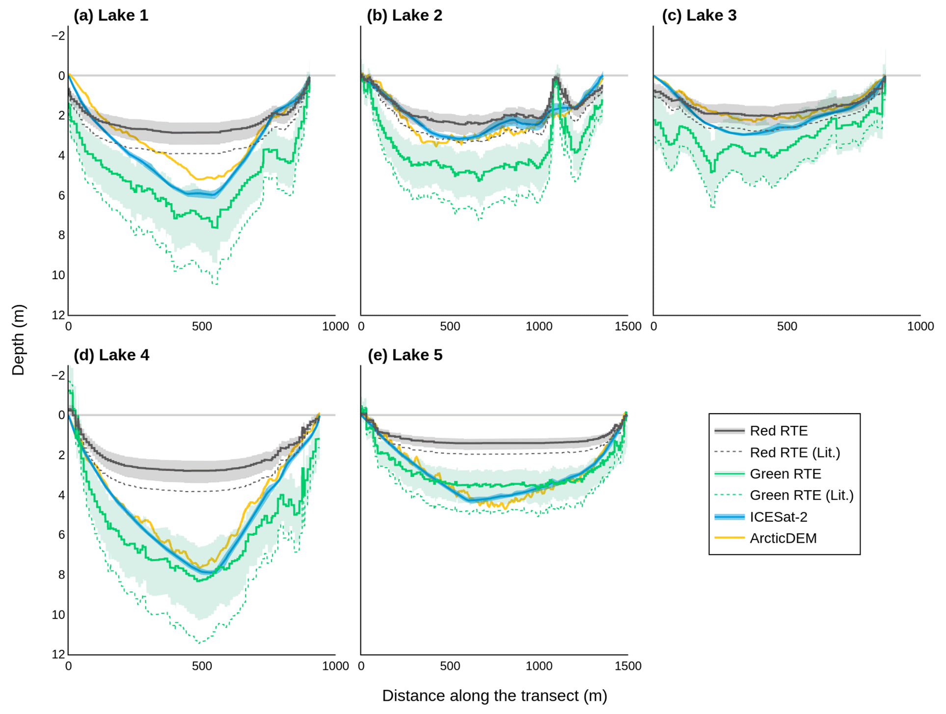
Figure 2 Supraglacial lake depth from the band-specific RTE, with both literature values and the values used for this study, ArcticDEM, and ICESat-2 along ICESat-2 transects. Depths achieved using the RTE with the literature values (red RTE (lit.), green RTE (lit.)) are shown for contextual reference. The uncertainties for each lake's band-specific RTE are calculated by co-varying all permutations of the RTE tuneable parameters. All uncertainties are calculated as 1 standard deviation. ArcticDEM absolute elevation accuracy is less than 5 m in the vertical plane (Noh and Howat, 2015). Lake 2 (b) exhibits a spike in both red-band RTE and green-band RTE depths at approximately 1200 m along the transect, which we attribute to a slight ice covering in the Sentinel-2 imagery. Transect locations are detailed in Fig. 1.

The red-band RTE depths plateau between 1 and 3 m, reaching their deepest depths at 2.87, 2.46, 2.04, 2.81, and 1.44 m for lakes 1, 2, 3, 4, and 5 respectively. This plateau typically results in an underestimation of maximum depth. In contrast, the green-band RTE depths show a systematic overestimation compared to ArcticDEM and ICESat-2. The RTE depths are deeper when literature values (Sneed and Hamilton, 2007; Georgiou et al., 2009; Pope et al., 2016) are used as opposed to our parameter values.

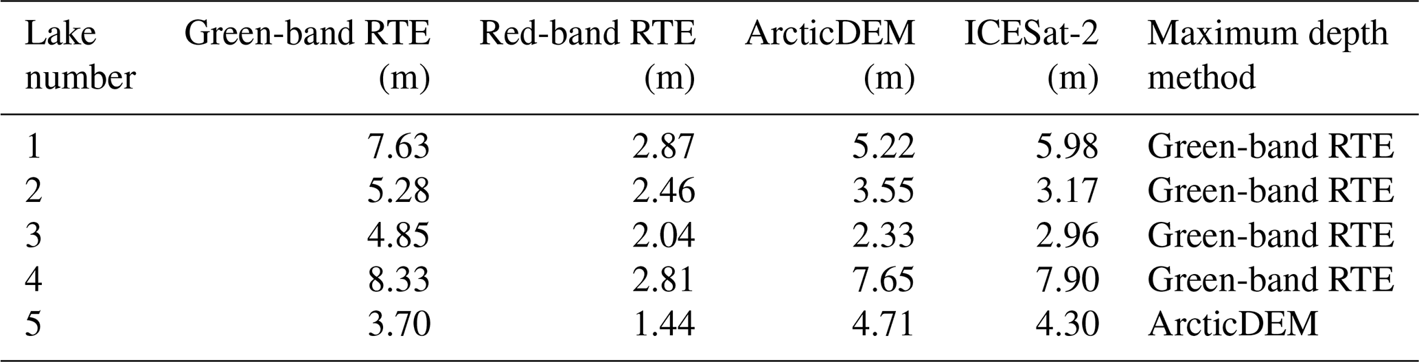
The maximum depths achieved by each method differ for each lake (Table 1). Here, we disregard the RTE depths retrieved using the literature values as these are shown only for contextual reference. For each of the five lakes, except Lake 5, the green-band RTE is the method which achieves the maximum depth for the lake. This is likely due to the observed overestimation of the green-band RTE.

Table 1 The maximum depths achieved by each method for the five lakes.

To explore the agreement between the different methods, we calculated the root mean square difference (RMSD) and Pearson's correlation coefficient for each method pairing at each of the 100 equally spaced points along which the ICESat-2 data were sampled (Fig. 3).

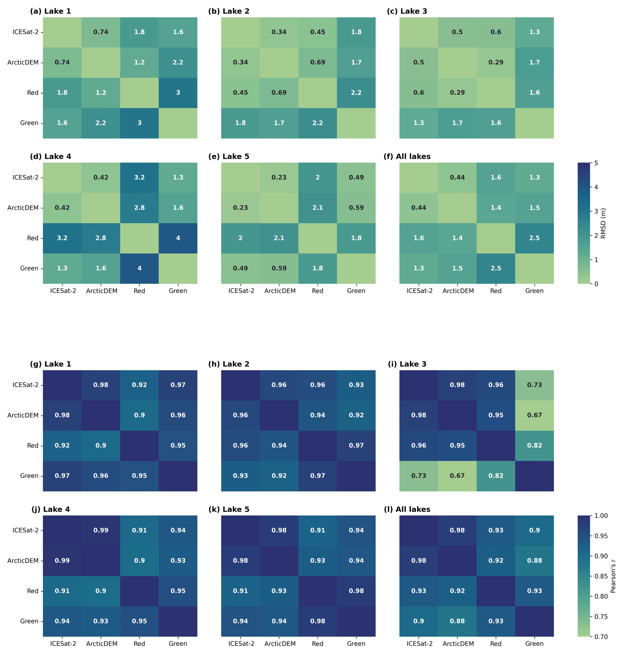
Figure 3 The root mean square difference (RMSD) and Pearson's correlation coefficients for each paired combination of depths derived from ICESat-2, ArcticDEM, red-band RTE, and green-band RTE. Panels (a)–(e) show the RMSD for Lake 1 to Lake 5, and panel (f) shows the average RMSD for all five lakes. Panels (g)–(k) show the Pearson's correlation coefficient for Lake 1 to Lake 5, and panel (l) shows the average Pearson's correlation coefficient for all five lakes.

From Fig. 3, the method pairing with the lowest RMSD is ICESat-2 and ArcticDEM for all lakes except Lake 3. For Lake 3, the method pairing with the lowest RMSD is the red-band RTE and ArcticDEM. On average, the ICESat-2 and ArcticDEM pairing has an RMSD of 0.44 m, and the method pairing with the highest average RMSD is the red-band RTE with the green-band RTE at an RMSD of 2.5 m. Additionally, our results indicate a high degree of agreement between the ArcticDEM depths and the ICESat-2 depths for Lake 5 (RMSD =0.23, r=0.98), enhancing our confidence in the lack of bathymetry change over the 11-month period between data acquisitions.

The Pearson's correlation coefficient of each of the method pairings is significant at p<0.001. However, some of the method pairings have stronger correlations than others. The method pairing with the strongest correlation for all of the lakes is ICESat-2 and ArcticDEM with an average r value of 0.98. The method pairing with the weakest correlation is different for each lake. For Lake 1 and Lake 4, the method pair with the lowest Pearson's r value is the red-band RTE and ArcticDEM (r=0.90 for both). For Lake 2 and Lake 3, the pair with the lowest r value is the green-band RTE and ArcticDEM (r=0.92 and 0.67 respectively). For Lake 5, the weakest correlation is for the pairing of the red-band RTE and ICESat-2 (r=0.91). The method pair with the weakest average Pearson's correlation is the green-band RTE and ArcticDEM (r=0.88), though this value is heavily impacted by the results from Lake 3.

3.2 ArcticDEM versus RTE: 2-D comparison of supraglacial lake depths

Next, we extend the 1-D analysis to two dimensions in a comparison between ArcticDEM and the RTE over the entire area of each lake (Fig. 4). Again, we find that the red-band RTE depths plateau at depths consistent with Fig. 2. Consistently with the findings from Fig. 2, the lakes exhibit a relationship between the green-band RTE depths and the ArcticDEM depths, where the green-band RTE overestimates depth in the deepest portions of the lakes. This is particularly evident in Lake 5 as its bathymetry is simpler than that of the other lakes. Additionally, there are notable depth underestimations of the green-band RTE in Lake 4 and Lake 5. These underestimations correspond to floating ice on the lake surface, which is not present in the ArcticDEM data. The green-band RTE depths do not have visible plateau depths for these lakes. Instead, this method again overestimates depths compared to ArcticDEM. Table 2 details the average difference in the green-band RTE and red-band RTE in comparison to ArcticDEM.

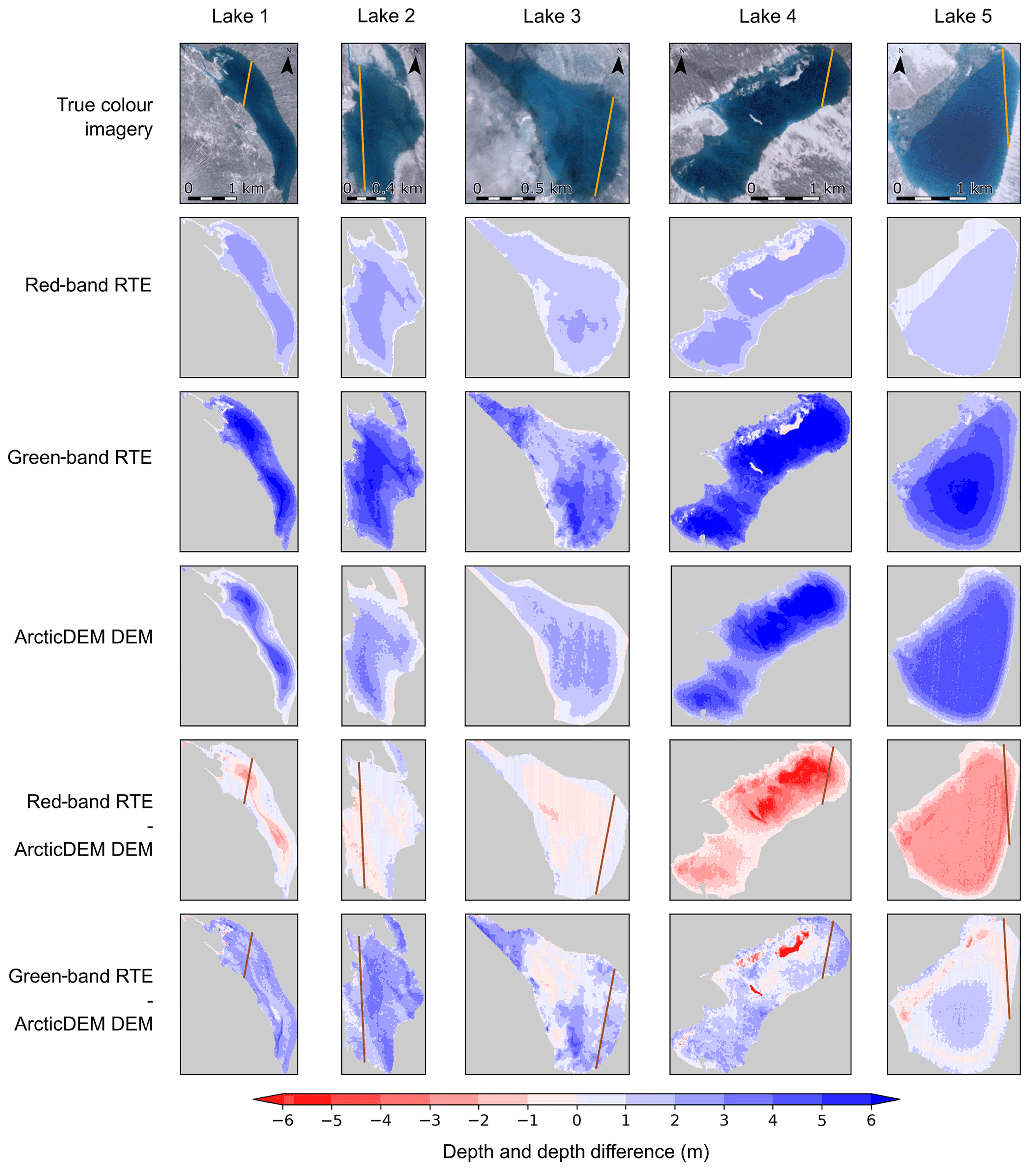
Figure 4 A comparison of red- and green-band RTE depths versus ArcticDEM depths in two dimensions. Each column shows results from one of our five study lakes, and each row shows information relating to a different retrieval method. The true-colour imagery is from Sentinel-2 (Table A1). ICESat-2 transects are shown in orange on the true-colour imagery and the depth difference plots.

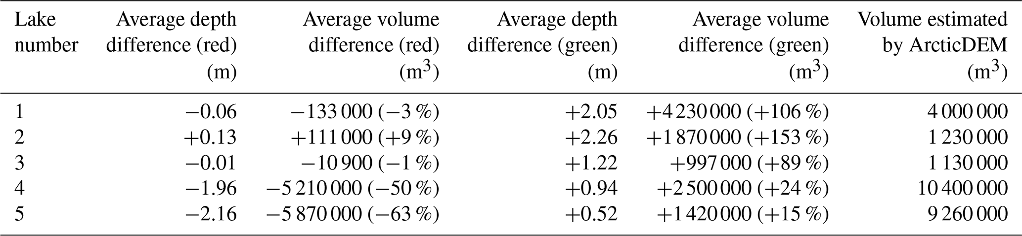
Table 2 The average overestimation by the green-band RTE and red-band RTE depths and volumes when compared to ArcticDEM DEMs for each of the five lakes. All volume estimates are shown to 3 significant figures.

To further explore the red-band RTE depth plateauing effect and to identify any noteworthy patterns in the relationship between green-band RTE depths and ArcticDEM depths, we compared the red- and green-band RTE depths versus the ArcticDEM depths for all ArcticDEM pixels across the five lakes (Fig. 5).

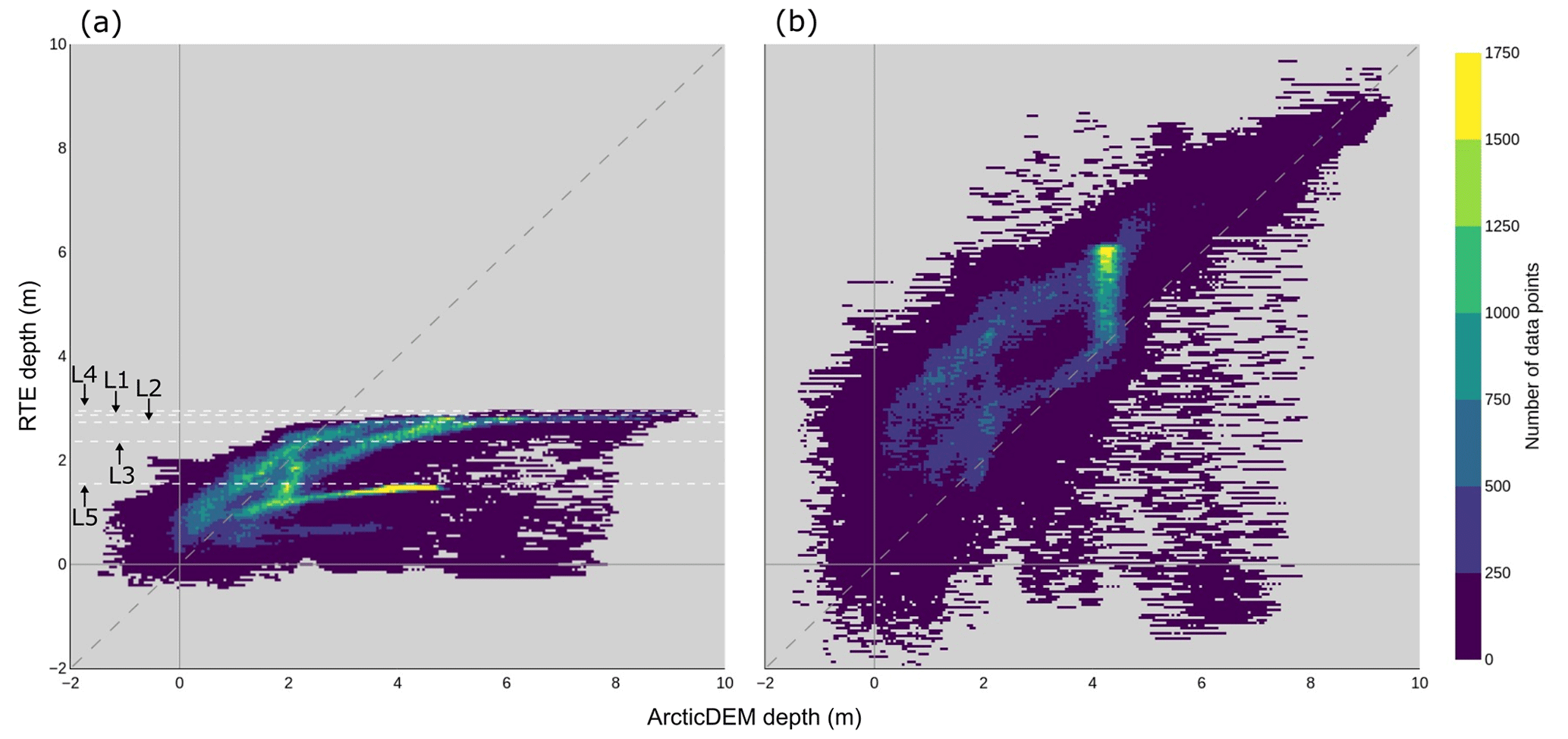
Figure 5 Density scatter plots of the depths derived from the red (a) and green (b) RTEs versus ArcticDEM depths for every pixel of the five lakes. The diagonal long-dashed lines represent one-to-one agreements between the depth datasets. The red-band RTE plateau depths are indicated by the labelled short-dash white lines in (a).

Figure 5 shows the relationship between the depth values of ArcticDEM, the red-band RTE, and the green-band RTE for every pixel of all five lakes. We find that the red-band RTE depth plateauing effect is clearly evident, with each of the lakes having a different plateau depth, as suggested in Figs. 2 and 4 (see dashed lines in Fig. 4a). This variance in red-band RTE depth saturation between lakes can be seen in the dense, elongated clusters of the red-band RTE cloud, each of which can be attributed to a different lake. We attribute the difference in plateau depth to the varying A_d values of the lakes, with red A_d values of 0.42, 0.46, 0.35, 0.58, and 0.57 for lakes 1, 2, 3, 4, and 5 respectively. Shallower depths (typically towards the lake edges, as seen in Fig. 4) agree relatively well when derived from the red-band RTE and ArcticDEM. However, as the lake gets deeper (towards the centre in most cases, as seen in Fig. 4), the agreement between the red-band RTE depths and the ArcticDEM depths decreases as a consequence of red-band saturation. The green-band RTE shows a different pattern to that of the red-band RTE. From the location of the cloud in relation to the XY line, we see that the green-band RTE typically overestimates depth compared to ArcticDEM. The plateau depths of the green-band RTE for these lakes are not visible, but the size of the cloud gives an indication of the larger spread of values compared to the red-band RTE.

3.3 RTE sensitivity analysis

To investigate the sensitivity of the RTE to the tuneable parameters in the equation, we computed the relationship between depth and R_w across the range of R_w values recorded over supraglacial lakes in our imagery (Fig. 6). We establish that, for the R_w values we observe in the 2019 lake inventory (Emily Glen, personal communication, 22 July 2022), the red-band RTE depths have a theoretical range of −1.66 to 2.68 m, whereas the green-band RTE depths have a much larger range of −7.23 to 11.76 m. This variation in range helps to explain why the red-band RTE plateaus. The maximum depth that could be achieved by the red-band RTE on 8 July 2019 from our study region was 2.68 m. The maximum depth retrieved by the red-band RTE for any of the five lakes was 2.87 m (Lake 1), which is due to the difference in date and thus the glaciological conditions of the ice sheet. Figure 6 is an indication of the limits to the green- and red-band RTEs on a specific date and not the absolute limits of the RTE. However, this analysis demonstrates that an empirical limit exists with regard to the depths achievable using both RTE approaches, which is shallower for the red band than it is for the green. Both the red- and green-band RTEs produce negative depths when the value of R_w is larger than the value of A_d. Physically, this means that the lake bottom albedo is lower than the reflectance of the pixel of interest. In practice, this only occurs (a) when the pixel of interest represents misclassified floating ice, such as in the green-band RTE plots for Lake 4 and Lake 5 (Fig. 4), or (b) as a result of uncertainty in A_d.

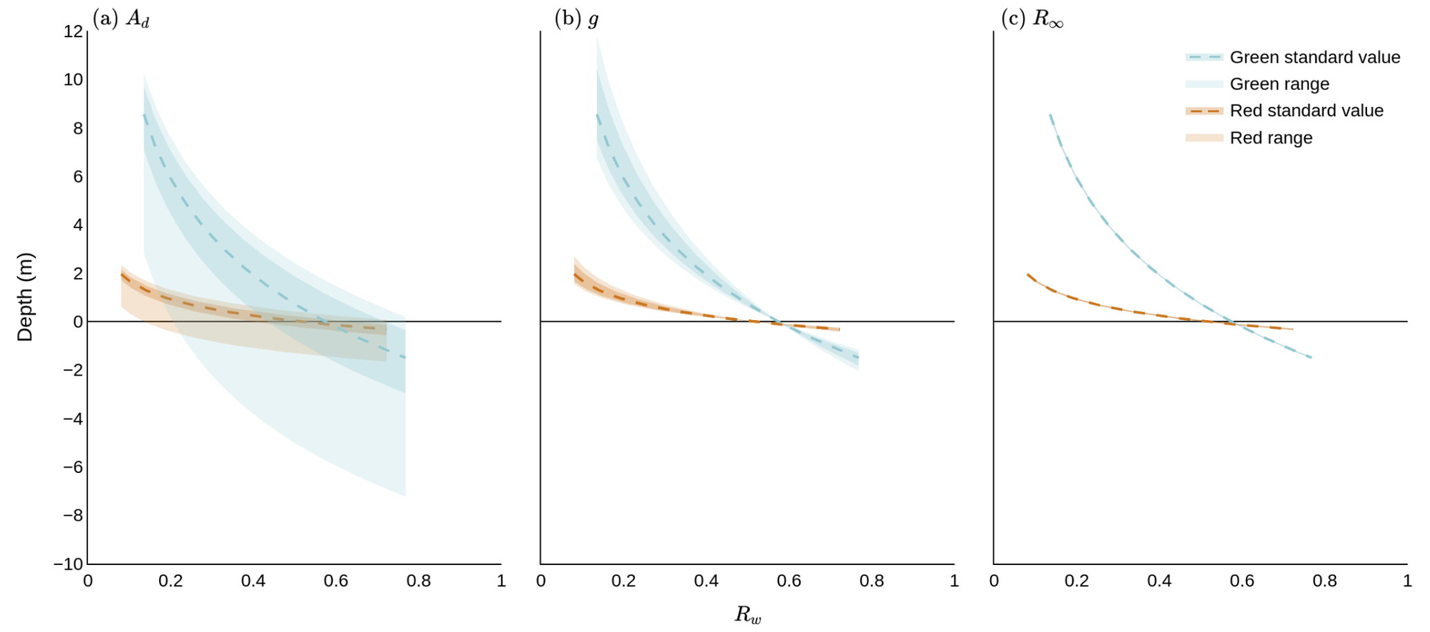
Figure 6 Sensitivity analysis of the RTE parameters within plausible ranges identified for each parameter (Appendix A3). Each panel shows the variability of lake depth, as given by Eq. (1), with measured surface reflectance: (a) when A_d is altered only, (b) when g is altered only, and (c) when R_∞ is altered only. When one parameter is altered, the other tuneable parameters are set to their literature value (see Sect. 2.2). R_w is varied over its observed range on 8 July 2019, where reflectance values were extracted using a lake inventory not generated explicitly for this study (Emily Glen, personal communication, 22 July 2022). Red standard value and green standard value are calculated using our approach to calculating A_d, g, and R_∞ (see Sect. 2.2). The darker-coloured shading indicates the uncertainty of these values. Red range and green range correspond to the possible depths achieved when upper and lower bounds are used for the parameter being varied. We note that in (c), the range and uncertainty of the depths are small and so appear as thin lines along the standard value lines.

The distribution of green-band RTE depths is broader than the distribution of depths for the red-band RTE in Fig. 5. We mainly attribute this to the variation in the range of possible depth values given in Fig. 6a, where the green-band RTE depth range is larger than that for the red-band RTE. The green-band RTE range is larger because of the A_d ranges of the lakes in the 2019 inventory, where A_d takes the range of 0.13–0.77 for red and 0.21–0.80 for green. When combined with the difference in band-dependent values of R_w and g, this results in a larger depth range.

4 Discussion

The RTE is the most common method applied at scale over the Greenland and Antarctic ice sheets to determine supraglacial lake depth (Sneed and Hamilton, 2007; Georgiou et al., 2009; Sneed and Hamilton, 2011; Banwell et al., 2014; Pope et al., 2016; Moussavi et al., 2016; Williamson et al., 2018; Moussavi et al., 2020). The RTE is widely used because the high volume of optical satellite imagery in the polar regions means locations that are lacking in other types of remotely sensed data can be studied. However, our analysis has shown that use of the RTE, in its current form, has some limitations. Due to the rapid attenuation of red light in water, the red-band RTE cannot sense deeper than approximately 3 m, with the precise saturation depths of the lakes being dictated by the A_d value. Therefore, evaluating the RTE with information from the red band means that depths from the portions of the lakes which are deeper than the red saturation point are being underestimated. As a result, when the red-band RTE is used to calculate lake depth, the total volume of water stored in lakes at the regional ice sheet scale is also underestimated.

Contrastingly, the use of the green band to evaluate the RTE leads to an overestimation of depth in the deepest portions of the lakes compared to ICESat-2 and ArcticDEM. From Fig. 6 we can see that the saturation depth of the green-band RTE is approximately 8–11 m. This depth is dependent upon the values of A_d and thus will be different for every lake. The saturation depths of the green-band RTE are not visible in Fig. 5 because the lakes are not deep enough for the physically constrained range of the green-band RTE to plateau. However, there are two distinctive patches of ArcticDEM depth saturation in the green-band RTE cloud of Fig. 5. These patches are portions of Lake 3 and Lake 5 which exhibit some noise within the DEM. Other spatiotemporally contiguous ArcticDEM data are unavailable for these lakes due to the sampling frequency of the dataset.

The average overestimations of the green-band RTE depths are typically larger than the average underestimations of the red-band RTE depths (Table 2), initially lending support to the use of the red-band RTE as opposed to the green-band RTE. However, the large variances in volume estimation between the green and red RTE depths and the ArcticDEM DEMs have contrasting implications with regard to both this assertion and one another. Use of the green-band RTE can lead to lake volume overestimations of 150 % relative to ArcticDEM, with similar overestimations expected at larger scales. This has further implications for our understanding of the role of meltwater in ice sheet dynamics and introduces a potential for exaggeration of the contribution of meltwater to localised ice velocities, which impacts our ability to predict ice-calving rates at marine-terminating glaciers (Melton et al., 2022). Conversely, use of the red-band RTE can lead to underestimations of 63 % of the lake volume compared to ArcticDEM, which would potentially yield contrasting implications for our understanding of ice sheet dynamics.

Due to the plateauing effect of the red-band RTE and the systematic overestimation of the green-band RTE, neither parameter selection (ours nor the literature's) results in good agreement with either ArcticDEM or ICESat-2 for deep lakes. Although previous studies have employed a band-averaging method (Pope et al., 2016; Williamson et al., 2018), our results show that there are effects present in different bands which may be masked in a band-averaging approach, such as the plateauing effect observed within the red-band RTE and consistent overestimations in the green-band RTE. Therefore, it is not appropriate to average the green-band RTE depths and the red-band RTE depths.

It is inconclusive which parameter selection is best for shallow lakes, highlighting the importance of parameter selection in the use of the RTE. With our parameter value choices, the green-band RTE appears to predict lake bathymetry in closer agreement with ArcticDEM and ICESat-2 than the red-band RTE. Conversely, using the methods reported in previous literature (Sneed and Hamilton, 2007; Banwell et al., 2014) to calculate each of the parameters leads to the conclusion that the red-band RTE, at depths lower than its saturation depth, is more accurate in gauging lake depth than the green-band RTE. It is clear from Fig. 6 that depth is largely insensitive to the choice of R_∞. Since our calculation of A_d is the same as that which is commonly used within existing literature (Sneed and Hamilton, 2007; Moussavi et al., 2020), we suggest that there is disagreement with respect to the best-performing band at depths lower than the saturation point of the red-band RTE because we use a different value of g. Specifically, a low coefficient of K_d leads to a low g value, which, as found in recent literature (e.g. Pope et al., 2016; Williamson et al., 2017), leads to larger lake depths. When this is combined with the green band in the RTE, it leads to a significant overestimation of depth, which can exceed 5 m, compared to the ICESat-2 and ArcticDEM depths (Fig. 2).

Using the parameter values commonly found in the literature (Sneed and Hamilton, 2007; Banwell et al., 2014), the red-band RTE predicts depth relatively accurately until it plateaus. This attribute makes it well suited for use with shallower lakes, such as those found on Antarctic ice shelves (Banwell et al., 2014). However, the calculation of A_d needs to be carefully considered. Specifically, if A_d is estimated from a ring of pixels around the edge of the lake (e.g. Sneed and Hamilton, 2007; Moussavi et al., 2020), then the presence of slush may adversely impact the derivation of a representative value. The differentiation of blue ice from slush on the Antarctic ice sheet is particularly difficult due to their structural and spectral similarities in satellite imagery (Moussavi et al., 2020; Dell et al., 2022). This makes the derivation of A_d even more complicated, and care should be taken when calculating A_d in the presence of blue ice due to the potential misidentification of slush (Dell et al., 2020). Figure 6 elucidates the importance of the choice of A_d within the RTE, wherein a small change in A_d translates into a large difference in estimated depth. Dell et al. (2020) estimated A_d from the sixth concentric ring of pixels around Antarctic lakes to reduce the potential impacts of slush on the RTE. In future work, methods of estimating A_d in both Greenland and Antarctica should be tested due to the importance of A_d in the RTE.

Although generally in closer agreement with one another than with the red- or green-band RTEs, ICESat-2 and ArcticDEM cannot be used to track surface water volumes at scale across the ice sheet because of limitations in their spatial and temporal sampling. For example, ICESat-2 acquires elevation measurements along 1-D satellite tracks, and lakes are 2-D features; furthermore, whilst ArcticDEM acquisitions are 2-D, they are sparsely sampled in space and time. Methods which exploit regularly acquired 2-D satellite imagery – such as the application of the RTE to optical satellite imagery – are thus needed to monitor the total volume of water held within lakes on the ice sheet surface and its evolution through time. ArcticDEM and ICESat-2 data are of most value for their potential to constrain these methods. For example, Datta and Wouters (2021) used ICESat-2 to constrain empirically derived estimates of lake bathymetry from Sentinel-2 scenes in western Greenland. With a larger amount of ArcticDEM and/or ICESat-2 data, we suggest that future research could combine multiple satellite bands (Adegun et al., 2023) and data sources as inputs to a machine learning model and generate a well-constrained depth detection product using a data-driven approach as opposed to the model-derived approach we use here.

The relatively weaker correlation between the RTE datasets and the observational datasets of ArcticDEM and ICESat-2 is likely a result of the uncertainty introduced by each of the RTE's tuneable parameters (Fig. 6). A_d, in particular, is affected by the potentially incorrect assumption that suspended or particulate matter in the lake is minimal (Sneed and Hamilton, 2011). This raises the issue of cryoconite holes on the ice sheet surface, which are known to lower the albedo (Hotaling et al., 2021). Cryoconite holes are formed when aeolian dust settles on the ice sheet. The albedo of the dust-covered area is lower than the surrounding ice so it heats up and melts the underlying ice, forming vertical shafts. The ponding of surface water partially cleans these cryoconite holes, resulting in the disbursement of the particulate matter into the lake. However, the method currently used to estimate A_d is assumed to accommodate this potential lowering of lake albedo. Therefore, if cryoconite was present in the lake basin, the ring of pixels used to estimate the lake bottom albedo would likely also contain cryoconite holes.

If the water column is affected by particulate matter, this would also affect the value of g (Brodský et al., 2022). Currently, g is calculated from K_d, the coefficient for the scattering of downwelling light in the water column. The K_d value is laboratory-derived from optically clear water, i.e. water that does not contain particulate matter. Consequently, the value of g would be incorrect for lakes which contain particulate matter, further limiting the generalisability of the RTE when it is used in such a scenario.

Currently, the limitations associated with red- and green-band RTE calculations have wider implications for other areas of cryospheric research, such as calculating hydrofracture likelihood and understanding fluctuations in local ice velocities. Lake volume is not the only control on the probability of lake hydrofracture, though it is reasonable to assume that the two things should be correlated. However, observational evidence of this correlation remains elusive despite large-scale studies of the phenomena (Williamson et al., 2018). It is possible that these large-scale studies found no evidence of a correlation between hydrofracture and lake volume, at least in part because of uncertainties in the RTE approach used to derive lake depth.

5 Conclusions

The Greenland ice sheet accommodates thousands of supraglacial lakes which form and reform every melt season. Current methods to estimate the volume of these lakes have either relatively poor spatio-temporal sampling or limitations in the accuracy with which they can retrieve lake depth. This study gives a detailed intercomparison of three methods which can be used to estimate lake depth – an integral component in the calculation of lake volume. Tracking the volume of water storage on the surface of the ice sheet is important for quantifying hydrofracture likelihood and determining the impacts of lake drainage on ice sheet velocities and requires ice-sheet-wide coverage and high temporal sampling to resolve seasonal dynamics.

Within this study, we found that two of the three methods considered, namely the ArcticDEM DEMs and the ICESat-2 laser altimetry approaches, have close agreement. However, these methods are spatially and temporally restricted, meaning they cannot be used to derive comprehensive estimates of surface water storage at the ice sheet scale. Our third method, which uses the Philpot (1987) RTE to derive depth from optical imagery, has relatively poor agreement with the other two methods, especially for deeper supraglacial lakes. We detected a plateauing effect in the red-band RTE which is caused by the rapid attenuation of light in the red band, suggesting that the use of this method will consistently underestimate the depths of lakes which are deeper than the lake-specific saturation limit. Within this study, the use of our RTE parameter values improved the ability of the green-band RTE to sense lake depth, and a comprehensive sensitivity analysis of the RTE's tuneable parameters leads us to believe that further alterations to the parameter calculation and/or equation could be undertaken to improve the method. Interestingly, the methods currently used within the literature to determine the parameter values appear to limit the accuracy of lake depth calculation using the green-band RTE within our five-lake sample. However, this is a case study of five lakes on the southwest Greenland ice sheet, and further work is required to understand whether this conclusion is generalisable to the whole ice sheet.

Nonetheless, the RTE is the only method which can currently be deployed at an ice sheet scale due to data availability constraints, meaning improvements to the method are paramount to its potential use as an accurate method for calculating lake depth. We suggest that future improvements to the current equation should focus on the calculation of A_d, which has been shown to have the greatest influence on the derived depths. However, the calculation of A_d also poses significant technical difficulties due to the issues in differentiating between water and ice in satellite imagery so care must be taken to ensure that new methods are robust and replicable at the ice sheet scale.

Appendix A

A1 Criteria to reduce the 2019 lake inventory

A 2019 inventory (Emily Glen, personal communication, 22 July 2022) of the maximum areal extents of all water bodies in the study region was used as the basis for selecting our five lakes, with the following characteristics used as the selection criteria:

• The water body is intersected by an ICESat-2 reference ground track (removed 7519 water bodies).

• The seasonal maximum water body area is greater than 1 km² but less than 10 km². This removes small water bodies which are absent in low melt years and large water bodies which are formed by the merging of smaller water bodies, thus leaving supraglacial lakes with dimensions that were representative of the regional average (removed a further 338 water bodies).

• The water body circumference is less than 30 km; i.e. it is not a highly elongated feature such as a stream (removed a further 28 water bodies).

These characteristics reduced the 2019 inventory from 7913 to 28. The lakes were then considered for their ICESat-2 data quality, where the highest quality translates to the basins which can be most easily delineated from ICESat-2 photon refraction (Sect. 2.3). Additionally, the 28 lakes were visually appraised for their level of activity (Sect. 2.2.1) to ensure that they drained and refilled. These comparisons identified five lakes for which depth could be derived for all three measurement techniques. The other lake basins from the initial subset of 28 could not easily be identified by ICESat-2 or could not be resolved using the ArcticDEM digital elevation models (Sect. 2.2.1).

A2 Input data

Lake-specific data were used during the course of this study, and the particulars of these data are detailed in Table A1.

Table A1 ArcticDEM, ICESat-2, and Sentinel-2 data used for depth retrieval in each of the five lakes. Acquisition dates are in bold text and are in the format YYYYMMDD.

A3 Selection of the RTE tuneable parameter values

Commonly, within the radiative transfer equation (RTE), the derivation of A_d is specific to a lake, or a regional average is used (Sneed and Hamilton, 2007). We have used an individual A_d for each lake because the reflectance of pixels surrounding supraglacial lakes can vary considerably. In our study, we calculated the A_d values specific to each lake. The red A_d values were 0.42, 0.46, 0.35, 0.58, and 0.57 for lakes 1, 2, 3, 4, and 5 respectively, and the green A_d values were 0.45, 0.49, 0.40, 0.60, and 0.58 for lakes 1, 2, 3, 4, and 5 respectively.

Our derivation of g is given by 2.75 K_d. In addition to this being an average of the potential range of g (2 K_d–3.5 K_d), this coefficient of K_d incorporates the concept that the value of K_d is dependent on depth (Kirk, 1989). This means an average value can be expected to retrieve a more representative depth than either the lowest or highest values in the K_d range.

Typically, R_∞ is calculated as the reflectance of the darkest pixel in a scene containing optically deep water (Sneed and Hamilton, 2007). Optically deep water, in the case of the Greenland ice sheet, consists of open ocean pixels. To reduce the impact of atmospheric effects, R_∞ is ideally calculated from either the same scene as the one containing the pixels of interest where there are open-ocean pixels or a concurrent neighbouring scene. However, it is not always possible to sample R_∞ from a concurrent neighbouring scene due to the location of the pixels of interest and/or cloud cover. In this case, a non-concurrent and/or non-neighbouring scene is chosen instead (Table A2). Sneed and Hamilton (2011) argued that all optically deep water has similar spectral characteristics, and, therefore, the precise method for determining this value negligibly affects the depths derived using the RTE. The findings of our RTE tuneable parameter sensitivity analysis agree with Sneed and Hamilton (2011) (Fig. 6).

Table A2 Sentinel-2 tiles used to retrieve R_∞ values for each lake. Acquisition dates are in bold text and are in the format YYYYMMDD.

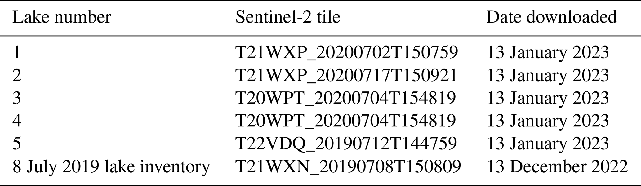
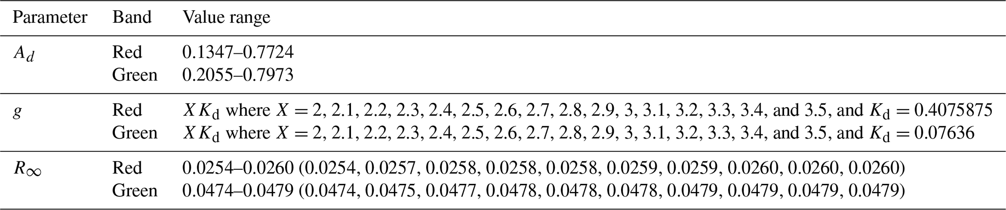
Table A3 The ranges of the tuneable parameters used to find the uncertainty of the 2019 lake inventory RTE depths.

A4 Plausible ranges of the RTE tuneable parameters

To calculate the uncertainty of the red- and green-band RTEs for the study lakes, we had to first understand the plausible ranges of the three tuneable parameters. The range of A_d was calculated as the range of R_w values of every pixel in the 30 m ring of pixels around each lake, as detailed in Sect. 2.2.1. The range of g was 1.5 to 3 K_d at 0.1 intervals for every lake, where K_d was calculated as the band-specific solution of Eq. (3) for the average a_w and $b_{\mathrm{m}}^{\mathrm{fw}}$ values from Smith and Baker (1981) for both the red and green optical bands of Sentinel-2. We calculated the ranges of R_∞ from the Sentinel-2 tiles detailed in Table A1. We manually appraised these scenes for spurious values caused by aeroplane overpasses and sediment contamination with the aid of a band combination to highlight snow and clouds (Band 1, Band 11, and Band 12 (coastal and aerosol, shortwave infrared (1610 nm), and shortwave infrared (2190 nm)). The R_∞ ranges consist of the R_w values of the 10 darkest pixels from each scene, which were true dark sea pixels.

Our study includes data from the sensitivity analysis that we carried out on the tuneable parameters using the plausible ranges of R_w from the 8 July 2019 lake inventory (Emily Glen, personal communication, 22 July 2022) (Fig. 6) (Table A3). The method of calculating A_d was slightly different due to the scale of the data. We calculated the range of A_d as the range of the average R_w values of the 30 m rings of pixels around all of the lakes in the 2019 lake inventory. We used the same method to calculate g and R_∞ as that which we used to calculate the uncertainty for the five study lakes. The scene from which we calculated the R_∞ range was spatiotemporally contiguous with the lake inventory data (Table A2).