Bounded and categorized: targeting data assimilation for sea ice fractional coverage and nonnegative quantities in a single-column multi-category sea ice model

A rigorous exploration of the sea ice data assimilation (DA) problem using a framework specifically developed for rapid, interpretable hypothesis testing is presented. In many applications, DA is implemented to constrain a modeled estimate of a state with observations. The sea ice DA application is complicated by the wide range of spatiotemporal scales over which key sea ice variables evolve, a variety of physical bounds on those variables, and the particular construction of modern complex sea ice models. By coupling a single-column sea ice model (Icepack) to the Data Assimilation Research Testbed (DART) in a series of observing system simulation experiments (OSSEs), the grid-cell-level response of a complex sea ice model to a range of ensemble Kalman DA methods designed to address the aforementioned complications is explored. The impact on the modeled ice thickness distribution and the bounded nature of both state and prognostic variables in the sea ice model are of particular interest, as these problems are under-examined. Explicitly respecting boundedness has little effect in the winter months, but it correctly accounts for the bounded nature of the observations, particularly in the summer months when the prescribed sea ice concentration (SIC) error is large. Assimilating observations representing each of the individual modeled sea ice thickness categories consistently improves the analyses across multiple diagnostic variables and sea ice mean states. These results elucidate many of the positive and negative results of previous sea ice DA studies, highlight the many counterintuitive aspects of this particular DA application, and motivate better future sea ice analysis products.

1 Introduction

Recent rapid Arctic change has emphasized the influence of sea ice on the global climate system, our incomplete understanding of its recent history, and many shortcomings of current sea ice models. The tide of interest in addressing these issues is well reflected in the accelerating application of data assimilation techniques in both sea ice reconstruction projects (Schweiger et al., 2011; Sakov et al., 2012; Mu et al., 2018a; Williams et al., 2022) and modeling studies (Zhang et al., 2021; Korosov et al., 2023). Data assimilation, or DA, is a set of objective methods through which observations of a system are blended with a modeled estimate of that system. Through this blending, DA injects the information gained via the observations, which are typically limited in space and can be intermittent in time, into a model capable of integrating that information forward in a spatiotemporally continuous, physically realistic manner. DA is most commonly used to obtain accurate initial conditions for numerical weather prediction models, but it can also be deployed in climate studies to reconstruct unobserved variables by synchronizing observable components of a system with nature (Brennan and Hakim, 2022) or to infer the correct parameterization values that should be used in Earth system models (Zhang et al., 2021). To date, most sea ice DA applications have employed ensemble Kalman filtering (EnKF) methods, a family of DA algorithms based on the Kalman filter (Kalman, 1960; Evensen, 2003; Houtekamer and Zhang, 2016). EnKF methods approximate the application of a true Kalman filter by sampling the system of interest using model ensembles. In practical applications, the adjustments made by these filters can be considered in four steps, which are outlined in Fig. 1 (adapted from Anderson, 2022, for a hypothetical adjustment of sea ice concentration, SIC). Firstly, the model is used to generate an ensemble of forecasts. Secondly, estimates of the observed quantities (e.g., SIC) are calculated from the model's state variables (e.g., categorized sea ice area fraction, A_ice,n). Thirdly, a version of the Kalman filter is applied to update the model's estimates of the observed quantity. Here, this will be referred to as observation-space incrementing. Finally, the adjustments made in observation space are used to determine the corresponding updates applied to the variables comprising the model state. This step is hereafter referred to as state-space regression. Together, observation-space incrementing and state-space regression are collectively known as filtering. Once filtering is complete, the updated model state is then used to initialize the next forecast step. All together, this process is referred to as a DA cycle.

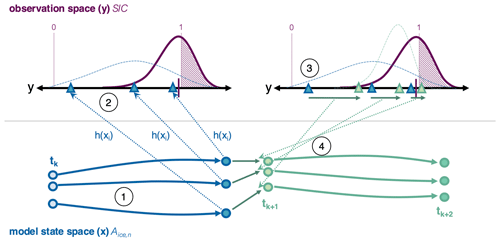
Figure 1 Schematic example of a data assimilation cycle in a sea ice application. A univariate example of a single data assimilation cycle is presented in four steps. In step 1, an ensemble of sea ice initial conditions (light-blue circles) is forecast forward from time t_k. In step 2 (dotted light-blue arrows), the ensemble of sea ice states is translated into an ensemble of observational estimates (blue triangles) using a forward operator, y=h(x). A continuous distribution, shown by the dashed light-blue line, is fit to the observation estimates and is compared to an observation, shown as a dark-pink hash on the y axis. The observational error distribution associated with that observation is shown using the dark-pink curve, and regions of the error distribution that imply nonphysical values are shaded with pink dots. In step 3, the model's observational estimates are adjusted by the data assimilation filter, based on the observation value and error distribution. The updated ensemble of observational estimates is shown using the green triangles. The amount that each ensemble member is adjusted is referred to as an observation increment (dark-green arrows). The observation increments are then used to determine the state-space increments, or the amount that the model state variables need to be adjusted to be consistent with the observation increment; this step (represented here by the dotted light-green arrows) is typically achieved using the linear relationship between observations and state variables to project the observation increment into model state space. Once the model state has been adjusted, the model is reinitialized to produce the next forecast from t_k+1 (light-green circles to dark-green circles). This figure has been reproduced with alterations from Anderson (2022).

Substantial nuance can arise in the cycling process depending on the characteristics of the system in question. This makes DA in any Earth system component model an intricate undertaking (and one that is often specifically tailored to the problem at hand). This is particularly true for sea ice, as sea ice models and observables unite many distinct challenges for DA in one system. Firstly, similar to atmospheric variables, such as cloud fraction, sea ice variables tend to be bounded. For example, ice cannot be negatively thick; sea ice concentration (the fraction of a model grid cell covered by ice) cannot fall below zero or exceed one. The Kalman methods applied to sea ice problems are based on assumptions that the model ensemble and the observation error distribution are normal distributions, which linearizes the filtering process. For system variables that are bounded, however, the use of normal distributions in the filtering algorithm can produce adjustments during observation-space incrementing that violate physical bounds (as illustrated in step 3 of Fig. 1). When these violations are corrected (typically through a post-processing step), the model ensemble mean is artificially shifted away from the bound, leading to a bias in the assimilation analysis. While non-Gaussian ensemble DA methods that avoid the use of normal distributions have been proposed, their application in high-dimensional systems has been limited (Riedel and Anderson, 2024; Anderson, 2010).

Secondly, the relationship between variables observed in the real world and modeled in the sea ice state is not straightforward. Sea ice observing systems measure variables such as SIC or sea ice thickness (SIT). However, SIC and SIT are diagnostic in modern sea ice models, which typically evolve through an ice thickness distribution (ITD). The ITD parameterizes sub-grid-scale thermodynamic and mechanical processes that are strongly dependent on ice thickness (Bitz and Roe, 2004; Chevallier and Salas-Mélia, 2012) by expressing the distribution of ice variables in a grid cell as functions of the ice thickness. In practice, the ITD describes a range of thicknesses within each grid cell and discretizes that range into an arbitrary number of thickness categories. Sea ice area and volume (and the snow volume atop the sea ice) are then similarly distributed across the thickness categories (Thorndike et al., 1975), and the evolutionary equations of the sea ice model are applied to each category individually. Observed SIC, SIT, and snow depth (SND) are aggregates of the “categorized” model variables of ice area (A_ice,n), ice volume (V_ice,n), and snow volume (V_sno,n), respectively; the latter three sets of variables represent the sea ice state. Thus, while estimates of SIC and SIT calculated in step 2 of the DA cycle are updated during observation-space incrementing when SIC or SIT observations are assimilated (step 3), the updates to the aggregate values are regressed out to each of the categorized variables during the state-space regression (step 4). The diagnostic SIC and SIT output at the end of the process are then reaggregated from the updated categorized state variables; their accuracy relies not only on the direct filter updates on the aggregate quantities but also on the model ensemble's relationship between the aggregated quantities and each of the categorized variables in the model state. Few studies have presented the impact of assimilating SIC or SIT on each of the model's categories individually, which raises the question of how well the process and impact of assimilating any observation into distribution-based sea ice models is understood. Recent work by Williams et al. (2022) documents the first attempt to assimilate an “observed” ice thickness distribution, rather than just an aggregate observation, into the sea ice component of a global climate model, with mixed results.

Both the non-Gaussian, bounded nature of sea ice and the relationship between aggregate observables and categorized state variables likely have important ramifications for sea ice DA, but they remain under-explored. This study presents a single-column sea ice data assimilation framework that allows for rapid hypothesis testing while also retaining the thermodynamic physics and ITD of a complex sea ice model. Within this idealized framework, the impact of using DA algorithms that respect the boundedness of sea ice model variables and observations is explored, as is the ITD response of the model when assimilating aggregate versus categorized area and thickness observations. The remainder of this paper is structured as follows: Sect. 2 provides an overview of the data assimilation framework and experimental methodology, Sect. 3 presents a discussion of the results generated by a suite of DA experiments targeting boundedness and categorized observations, Sect. 4 contextualizes this work with respect to more practical sea ice DA applications, and Sect. 5 provides conclusions.

2 Model and methods

The data assimilation framework used in this study couples the Data Assimilation Research Testbed (DART; Anderson et al., 2009) to Icepack (version 1.3.1; Hunke et al., 2022), the column physics package of the CICE sea ice model, which is widely used as the sea ice component of several Earth system models. Icepack can be run in a stand-alone configuration as a sort of single-column model and is reviewed in Sect. 2.1. DART is discussed in more depth in Sect. 2.2. In keeping with naming conventions developed in coincident work (Riedel et al., 2024), the collective assimilation system is referred to as CICE-SCM-DART. All experiments performed for this study are observing system simulation experiments (OSSEs), which assimilate synthetic observations derived from a randomly selected (and subsequently withheld) member of the sea ice ensemble. In each experiment, the randomly selected member represents a known “true” state against which the efficacy of assimilating observations of various types and with various uncertainties can be evaluated. For simplicity, a sea ice quantity produced by CICE-SCM-DART is hereafter differentiated from the assimilated synthetic observations using the terms “modeled” and “observed”, respectively.

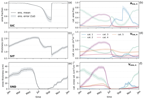
Figure 2 The FREE ensemble's three aggregate variables and the state variables from which they are derived. The aggregate variables shown on the left (a, c, and e) (SIC, SIT, and SND) are the area-weighted sums of the categorized state variables (category ice area, ice volume, and snow volume) on the right (b, d, and f). There are five thickness categories, where category 1 refers to the thinnest ice (0–0.64 m) and category 5 refers to the thickest ice (4.57 m and thicker). Dark lines indicate the ensemble mean of each variable, whereas lighter shading represents the ensemble standard deviation around the mean.

2.1 Icepack

Icepack is maintained as the column physics module of CICE, with consistent thermodynamics, mechanical redistribution, and tracer support. For use in the CICE-SCM-DART framework, 30 instances of Icepack are forced by unique atmospheric conditions extracted from randomly selected members of a recent large-ensemble reanalysis product (Raeder et al., 2021). Each instance of Icepack uses the mushy thermodynamics scheme (ktherm = 2) and linear ITD remapping options (kitd = 1), as well a delta-Eddington shortwave radiative transfer scheme and the empirical CESM melt pond scheme. Dynamical forcing to the column is provided by sea ice deformation rates obtained from the SHEBA field campaign (Lindsay, 2002). The number of categories used in the ITD is set to a value of 5. The snow grain radius parameter (R_snw) is set to a value of −2. This choice, which is among the default values of R_snw used when CICE is coupled to an atmospheric model, avoids rapid refreezing events during the melt season that lead to unreasonably high summertime sea ice concentrations given the atmospheric forcing conditions. All other sea ice model parameters are held at their default values. Each instance of Icepack is also coupled to a slab ocean; the ocean initial conditions and heat flux convergence forcing are identical for all 30 members and are derived from the ocean component output of a fully coupled historical simulation from the Community Earth System Model (CESM2). Both the ocean and atmosphere data sets represent grid cells nearest 75.54° N, 174.45° E, a point that straddles the East Siberian and Chukchi seas and experiences seasonal sea ice advance and retreat. The use of a seasonal location for this case study allows us to evaluate the performance of data assimilation near the upper and lower bounds of sea ice concentration.

The ensemble is spun up over a 10-year period during which the atmospheric conditions cycle continuously over the year 2011, allowing the sea ice simulations to diverge in response to atmospheric variability. No assimilation occurs during this period. Once spin-up is complete, a final yearlong ensemble simulation is produced as a control case for the assimilation experiments. This simulation, which is also free of any assimilation, is hereafter referred to as the FREE case and is outlined in Fig. 2. Both categorized state variables (Fig. 2b, d, f) and their diagnosed aggregates (Fig. 2a, c, e) are shown, as both can be observed and adjusted by assimilation.

2.2 DART

DART is a modular data assimilation framework developed by the Data Assimilation Research Section at the National Science Foundation (NSF) National Center for Atmospheric Research (NCAR). DART interfaces with many models that range in complexity from the Lorenz three-variable chaotic model to the Community Atmosphere Model (CAM6), the atmosphere component of the CESM2 climate model. DART implements the four-step cycling approach outlined in Sect. 1: forecast, conversion to observation space, observation-space incrementing, and state-space regression (Fig. 1). DART currently includes 10 filtering algorithms, encompassing variants of the ensemble Kalman filter (EnKF; Evensen, 2003) and several kernel and particle filter options. The default filter, the ensemble Kalman adjustment filter (EAKF; Anderson, 2001), implements a square-root filtering approach that increases the stability and efficiency of assimilating with smaller ensemble sizes compared with a traditional EnKF. Like most traditional ensemble filtering approaches, the EAKF makes Gaussian assumptions for the model ensemble and the observation error distributions.

Anderson (2001)Riedel et al. (2024)Anderson (2023)

Table 1 QCEFF filter components. This table includes the distributions used to represent the model ensemble in observation-space incrementing and state-space regression, the observation error distribution associated with each filter, any DART filter equivalents, and relevant references.

Recently, Anderson (2022) developed a novel filtering approach known as the quantile-conserving ensemble filtering framework (QCEFF). QCEFF alters the process by which the updated ensemble is sampled from the analytical blend of the model ensemble distribution and the observation error distribution. As a result, DART users can prescribe non-Gaussian distributions that may better represent the model ensemble or observation of interest. For example, in the sea ice problem, QCEFF allows the user to prescribe distributions that respect sea ice bounds, a level of detail that cannot be attained by EAKF or other Gaussian filters. In this framework the user can prescribe a distribution for each observable or state variable, as well as being able to differentiate the distribution used for observation-space incrementing versus state-space regression; this kind of choice allows the user to tailor the DA framework to the problem at hand in every step of the filtering process. When the user prescribes normal distributions in the QCEFF framework, the solution collapses to the EAKF.

We employ QCEFF to examine whether explicitly accounting for sea ice boundedness can improve sea ice assimilation analyses. To do so, we compare four different filtering approaches, outlined in Table 1. These filtering approaches use varying combinations of normal and piecewise rank histogram distributions in the observation-space incrementing and state-space regression steps of the filter. Piecewise rank histogram distributions prescribe no more information about the distribution of the sea ice system than can be gained from the discrete ensemble members themselves and can capture physical bounds; their use in step 3 of the DART filtering algorithms and for sea ice applications is discussed in more detail in Anderson (2022), Riedel and Anderson (2024), and Riedel et al. (2024). The use of bounded normal rank histogram (BNRH) distributions in state-space regression (step 4) of the QCEFF enforces appropriate bounds by way of a series of transforms in probit and probability integral space. This aspect of the QCEFF also more deftly handles nonlinear relationships between observed quantities and modeled state variables and is addressed in depth for idealized cases in Anderson (2023).

2.3 Experimental setup

All experiments performed for this study follow a perfect-model observing system simulation experiment (OSSE) protocol (Zhang et al., 2018; Riedel and Anderson, 2024; Riedel et al., 2024), a methodology typically used to identify the impact of assimilating a set of proposed or synthetic observations. The use of synthetic observations allows for a close inspection of DA filter performance given a set of observations derived from a known state. Here, several different kinds of synthetic sea ice observations are assimilated using each of the filter types listed in Table 1. Each experiment was branched from the end of the ensemble spin-up period, assimilated observations for a year, and was then compared to the FREE case. The assimilation experiments presented in the results are listed in Table 2.

Table 2 Assimilation experiments. Filter refers to the filter type used (see Table 1); Obs. kind refers to the type of observation assimilated. Observation error estimates associated with each observation kind are shown in Table 3.

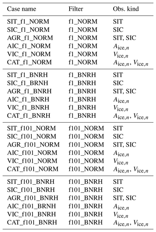
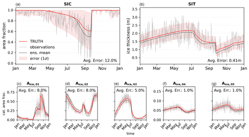
Figure 3 Synthetic observations extracted from a randomly selected member of the FREE ensemble. The observations assimilated are shown using gray lines for SIC (a), SIT (b), and category ice area (A_ice,01–A_ice,05) in panels (c)– (g). The TRUTH from which the observations are generated is shown using the solid red line, while the FREE ensemble mean is shown using the dashed black line. The observation error standard deviation (1σ) is shown as red shading around TRUTH.

The synthetic observations assimilated (a subset of which are presented in Fig. 3) are identical across experiments and are derived from a randomly selected ensemble member of the FREE case, which is hereafter referred to as TRUTH. To capture the basic influence of observation instrument and algorithmic errors on sea ice DA, observation error magnitudes are estimated based on previous work (Zhang et al., 2018; Riedel et al., 2024) and expressed as a function of the daily TRUTH value (listed in Table 3). The error magnitude, which can be thought of as the second moment of a probability distribution, is then used to determine a prescribed observation error distribution (OED) centered on the TRUTH estimate of the observation. Each daily observation is then randomly sampled from the OED. The resulting observation time series thus captures reasonable noise around the known TRUTH. In ensemble Kalman DA studies preceding QCEFF, the OED was assumed to be a normal distribution around TRUTH values. Here, the OED is set as a bounded normal distribution, thereby accounting for the physical realities of sea ice observations.

Table 3 Observation error estimates as a function of observation kind. Obs. kind refers to the type of observation assimilated. Obs. error refers to the formula used to determine an individual error estimate for each observation at each time step. a_n and v_n refer to the respective area and volume in the nth ITD category; $\stackrel{\mathrm{‾}}{h_n}$ refers to the midpoint thickness in the same category. h_R and h_L are the respective upper- and lowermost thickness bounds used to define the nth ITD category.

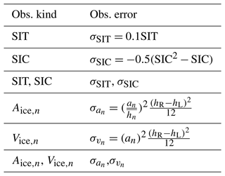
Aggregate observation values extracted are SIT and SIC. The variance of the observation error distribution for each synthetic SIT observation is a linear function of the true SIT value on the order of tens of centimeters. Observation error variance for synthetic SIC observations is a parabolic function of the true value on the order of 10 % of the grid cell area. As a result, observation error magnitudes when SIC declines in the summer months can be quite large, implying a plausible range of observations that may exceed the SIC upper bound of one. When used to determine a bounded OED that does not exceed one, these large errors lead to summer SIC observations that are biased low relative to TRUTH. The ramifications of this bias are discussed in Sect. 3 and 3.1.

Synthetic categorized observations are also drawn from each of the model's area and volume ITD categories (A_ice,n and V_ice,n, respectively) and are always assimilated together (i.e., assimilating A_ice,n indicates that each of the five area categories are assimilated simultaneously). Categorized area and volume observation error variances are assumed to follow a uniform distribution in each category, weighted by the total area (and midpoint thickness, in the case of volume observations) of that category. These errors are therefore generally less than 10 % of the true category value (Fig. 3).

Because sea ice ensembles perturbed only by differing atmospheric conditions (and not by varying model parameters) are generally under-dispersive with respect to SIC (Zhang et al., 2018; Williams et al., 2022; Riedel and Anderson, 2024), we apply enhanced spatially varying state-space prior inflation (El Gharamti et al., 2019) in each experiment. While the benefits of the spatial variation are lost on our application, the algorithm used implements an inverse gamma function that enables an increase or decrease in ensemble spread and outperforms alternative inflation algorithms in some cases (El Gharamti et al., 2019). The applied inflation uses a damping factor of 0.9, a lower standard deviation bound of 0.6, and a maximum per-time-step standard deviation change of 5 %.

Spatial localization is practically uninformative in a single-column application, but we explore the effect of “category localization” in the experiments assimilating A_ice,n or V_ice,n. Category localization weights the covariance values between variables in different ITD categories by zero. As a result, an observation from any of the individual ITD categories is prevented from updating any state-space variable that is not also in the same ITD category. In theory, this type of localization should limit the effects of potentially spurious relationships between categories and allow us to more reasonably treat category error variances as uncorrelated.

Finally, as DA is not guaranteed to respect the physical bounds of a system, it is common to use some post-processing method to correct any nonphysical adjustments made by the filter. DART includes three post-processing options for sea ice: two mass-aware rescaling approaches and one rebalancing method that has been adapted from a CICE internal function (Riedel and Anderson, 2024; the current default in CICE-SCM-DART). All experiments in Table 2 make use of this default rebalancing option, which redistributes the ice fractional coverage in each category to ensure that the thickness bounds are respected and then calculates consistent ice and snow volumes, salinities, and enthalpies once the updates have occurred. Each experiment was rerun using the other two post-processing methods; however, as no significant differences resulted, those additional experiments are not discussed here.

2.4 Evaluative metrics

To evaluate results, the ensemble means of the FREE case and each experiment (EXP) in Table 2 are compared to TRUTH using three metrics: mean absolute error (MAE), root-mean-square error (RMSE), and the coefficient of efficiency (CE). The presented definitions are generalized such that EXP and TRUTH may represent the experiment ensemble mean and reference “true” value, respectively, of any of CICE-SCM's state or diagnostic variables. In this study, these metrics are only applied to SIC, SIT, and SND.

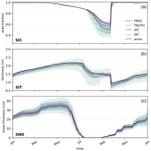
Figure 4 Assimilating with unbounded algorithms. The results of using an unbounded filter (f1_NORM) to assimilate SIC (solid teal line), SIT (solid blue line), or category area observations (solid purple line) are shown for modeled SIC (a), SIT (b), and SND (c). The black line represents the FREE case (without assimilation), whereas the thin red lines are the randomly selected TRUTH. For the results shown, thick lines are ensemble means, while shading represents the ensemble standard deviation around the mean. Observations are assimilated at daily intervals throughout atmospheric forcing year 2011.

MAE measures the average discrepancy between the forecast (FREE or EXP) and TRUTH over the course of the forecast period and is defined as follows:

$$\begin{array}{}\text{(1)}& \text{MAE}=\sum _i^n{\displaystyle \frac{|{\text{EXP}}_i-{\text{TRUTH}}_i|}{n}},\end{array}$$

where n indicates the number of time steps in the forecast period. RMSE, defined as

$$\begin{array}{}\text{(2)}& \text{RMSE}=\sqrt{\sum _i^n{\displaystyle \frac{({\text{EXP}}_i-{\text{TRUTH}}_i{)}^{\mathrm{2}}}{n}}},\end{array}$$

also evaluates how the forecast deviates from TRUTH but additionally provides a sense of whether the average discrepancy tends to include large outliers. The RMSE is therefore always greater than MAE, but the difference between the two will be close to zero in a desirable forecast.

The CE (Nash and Sutcliffe, 1970) measures forecast skill compared to TRUTH by evaluating how efficient the forecast is as a model of the observed system's mean and variance. It is calculated using

$$\begin{array}{}\text{(3)}& \text{CE}=\mathrm{1}-{\displaystyle \frac{{\sum }_i^n({\text{EXP}}_i-{\text{TRUTH}}_i{)}^{\mathrm{2}}}{{\mathit{\sigma }}_{\text{TRUTH}}^{\mathrm{2}}}}\end{array}$$

and lies between −∞ and 1. A CE equal to 1 indicates a perfect match between the forecast and the TRUTH (the numerator in the second term of Eq. 3 is 0), whereas a CE of 0 reflects a forecast that performs only as well as climatological prediction (the deviations of the experiment from TRUTH are equal to the variance of the TRUTH around its mean). A negative CE indicates that the forecast is not skillful. In general, the more positive the CE value, the better the forecast.

To couch results in a generalized framework, differences in the MAE and RMSE between the EXP forecasts and the FREE forecast are evaluated using a percent reduction approach, thereby diagnosing the impact of assimilating observations relative to forecast with no assimilation. For example, percent RMSE reduction (pRMSE) due to assimilating observations is calculated as

$$\begin{array}{}\text{(4)}& \text{pRMSE}=\mathrm{100}\times {\displaystyle \frac{{\text{RMSE}}_{\text{FREE}}-{\text{RMSE}}_{\text{EXP}}}{{\text{RMSE}}_{\text{FREE}}}}.\end{array}$$

Many of the experiments performed for this work have a high CE, due to the idealized nature of single-column OSSE experiments. In order to highlight the impact of assimilation, we choose to quantify this metric as a CE increase (iCE):

$$\begin{array}{}\text{(5)}& \text{iCE}={\text{CE}}_{\text{EXP}}-{\text{CE}}_{\text{FREE}}.\end{array}$$

In order to understand whether (a) assimilating with different methods and different variables leads to meaningful adjustments toward TRUTH and (b) any combinations of observations and filters significantly outperform the others over the course of the year, statistically significant differences between the ensemble mean time series of each EXP, FREE, and TRUTH are diagnosed using Welch's t test.

3 Results

The results of assimilating observations of SIT, SIC, and categorized area A_ice,n with an unbounded DA filter (f1_NORM) are presented in Fig. 4. This case illustrates that CICE-SCM-DART replicates the results of larger modeling studies discussed in Sect. 1. Assimilating SIT observations results in better sea ice analyses year-round than assimilating SIC observations, which have an impact only during the summer months when the model ensemble is capable of capturing variations in sea ice cover. In fact, assimilating SIC observations appears to have a negative impact on modeled SIC in Fig. 4, although this is because our method for producing synthetic SIC observations – which are derived using a bounded normal OED – generates SIC observations that are biased low relative to the TRUTH (Fig. 3). This is particularly true in the summer months when modeled SIC in TRUTH is comparatively low and the prescribed observation error variance is large (Table 3).

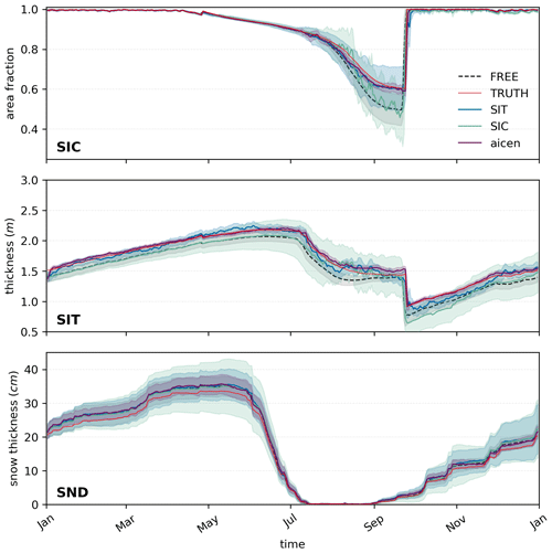
Figure 5 Assimilating with bounded algorithms. Same as Fig. 4 but for a case in which observations are assimilated using the f101_BNRH (fully bounded) filter.

Unlike the unbounded case (Fig. 4), the bounded OED is appropriately accounted for and the results lie close to the FREE mean when observations are assimilated with a fully bounded filter (f101_BNRH) (Fig. 5). From this, we conclude that, while a bounded filter does not overcome the limited efficacy of assimilating SIC observations, respecting boundedness in the assimilation does prevent the introduction of additional bias related to assumptions about the OED. We also note that assimilating SIC observations with $\mathrm{1}/\mathrm{10}$ of the error prescribed in Table 3 does shift the resulting modeled SIC closer to TRUTH (not shown), although whether such small-magnitude errors are reasonable is a separate discussion left for other work. In contrast, assimilating A_ice,n observations performs at least as well as assimilating SIT observations in the unbounded case, and this will be discussed in more depth later.

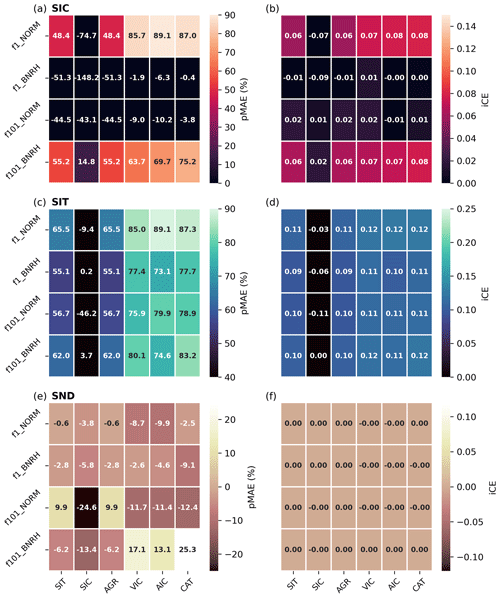
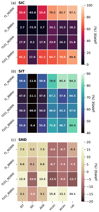
Figure 6 Bias reduction and model efficiency as a function of filter type and observation kind. Percent MAE reduction (pMAE) (a, c, and e) and CE increase (iCE) (b, d, and f) relative to the FREE forecast as a result of assimilating various observation kinds (x axis; see Table 2 for definitions) with each filtering method (y axis). Results are shown for modeled SIC (a, b), SIT (c, d), and SND (e, f). In general, lighter-toned colors indicate a more beneficial impact due to assimilation than darker-toned colors. The number values indicate the specific pMAE or iCE associated with each experiment.

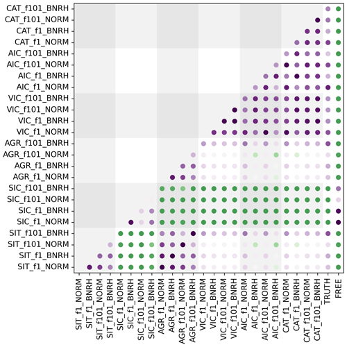
Figure 7 Significant differences between experiments. The significance of deviations between each assimilation experiment, TRUTH, and the unassimilated FREE ensemble mean are shown. The color gradient represents p values for the statistical difference between each experiment shown on the x axis with respect to each experiment shown on the y axis. The rightmost columns show the p values for differences from TRUTH and the FREE case. Purple shades indicate a insignificant difference at a p value of 0.05, while green shades indicate that the two cases in question differ significantly at a p value of 0.05.

A more succinct comparison of the experiments listed in Table 2 is presented in Fig. 6. In terms of modeled SIT, we find that the assimilation of any observation that either explicitly or implicitly (through categorization in the ice thickness distribution) contains information about ice thickness reduces MAE by between 70 % and 90 % and improves the CE score by ∼ 0.1, regardless of the filter used. Experiments assimilating SIT and categorized observations are not significantly different from TRUTH, although they are all significantly different from the FREE ensemble mean (Fig. 7).

Adjustments to modeled SIC are more variable. The relative lack of improvement as a result of assimilating SIC compared with SIT is not a novel result (Blockley and Peterson, 2018; Kimmeritz et al., 2018; Mu et al., 2018b; Zhang et al., 2018; Fiedler et al., 2022; Williams et al., 2022), but a good confirmation that the grid-cell-level responses investigated here are reminiscent of sea ice DA studies that use more traditional ensemble filtering methods and assimilate on larger grids. For modeled SIT and SND, there is very little variation in the results as a function of the filter used (Fig. 6). For modeled SIC, larger pMAE tends to stem from cases using totally unbounded or totally bounded filtering (f1_NORM or f101_BNRH, respectively) algorithms or when assimilating categorized observations.

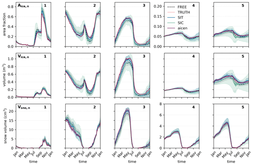
Figure 8 Category-level impact of assimilating with unbounded algorithms. Same as Fig. 4 but for each of the model's five ice categories (top row), volume (middle row), and snow volume categories (bottom row). TRUTH (the thin red line) may be difficult to identify in some panels, as the cases assimilating SIT and A_ice,n (solid blue and purple lines, respectively) lie very close to TRUTH.

Finally, modeled SND is degraded by the assimilation of sea ice observations in all cases, except those which assimilated categorized observations with a totally bounded filter. Assimilating snow depth observations has been shown to improve snow estimates in large models, when compared with cases in which snow was updated only via post-processing (Riedel and Anderson, 2024), as well as in a single-column model when assimilated alongside sea ice observations (Riedel et al., 2024). In the experiments performed here, categorized snow (V_sno,n) is a state variable that is updated via regression with the model's observed quantities, but no snow observations are assimilated. The general inefficacy of sea ice observations to reduce snow bias likely derives from an ensemble relationship between sea ice variables and categorized snow that produces too much late-winter/early-spring snow on thicker ice and too little on thinner ice (Fig. 8).

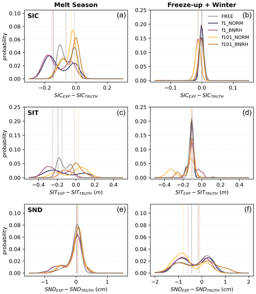
Figure 9 Seasonal impact of using bounded filters when assimilating SIC observations. The normalized probability density functions of the differences between the EXP mean and TRUTH in each assimilation cycle are shown for modeled SIC (a, b), SIT (c, d), and SND (e, f), along with their respective sample medians (dashed vertical lines). The dark-gray distribution in each panel represents the difference between the FREE ensemble mean and TRUTH as a reference. The differences are divided into the melt season (a, c, and e; 1 July–15 September) and the rest of the year (b, d, and f) and highlight the positive seasonal impact of using bounded algorithms – in the melt season, the distributions are shifted closer to an EXP–TRUTH difference of zero when a bounded filter is used (yellow lines) than when an unbounded one is used (pink lines). This effect is most prominent in the melt season months, as the uncertainties associated with the assimilated SIC observations are largest in these months; thus, the bounded synthetic observations are more biased relative to TRUTH during this period. The bounded algorithms correct for this appropriately.

3.1 Boundedness

In general, we find that the metrics in Figs. 6 and 7 have a rather weak dependence on whether or not the filter respects bounds for modeled SIT and SND, especially when compared to the obvious dependence on the kind of observation assimilated. There is essentially no dependency highlighted by iCE and only minimal variation in pMAE. In terms of modeled SIC, however, the impact of using a bounded filter is more apparent (Fig. 9). The use of bounded rank histogram distributions in observation-space allows the filter to correctly infer the bounded nature of the observation error distribution (which respects the physical upper bound of 1 for SIC) and its relationship to TRUTH. The adjustments thus avoid degrading modeled SIC and lead to a positive annual pMAE (Fig. 6) and reduced bias relative to TRUTH, particularly in the melt season, when SIC observation errors are particularly large (Figs. 9, 5). The poor performance of the intermediary filters (f1_BNRH and f101_NORM) to constrain modeled SIC (Fig. 6) can be attributed to their inability to adjust SIC to total ice cover in the winter months (not shown).

The underperformance of the bounded filters with respect to SIC is likely due to the nature of the model state variables (categorized ice area, ice volume, and snow volume). Recall that the values being diagnosed (SIC, SIT, and SND) are calculated from categorized quantities using forward operators, but they are not themselves state variables. This formulation leads to an issue with properly constraining modeled SIC. In the first step of the assimilation, bounds are placed on the observed quantity, SIC, which is calculated by applying a forward operator (a simple summation) to the model's forecast of the category area fractions in the ITD. Observation-space incrementing respects the bounds prescribed on the observable. However, in the second step of the assimilation, the increment calculated between the observation and the model's estimate of the observed quantity is mapped back onto the category-based state variables using regression. This step also respects boundedness, but it must rely on bounds prescribed by the user for each of the state variables. The only objective bounds that can be placed on each individual category area fraction are [0, 1], meaning that the regression of the observation-space increment can update each of the individual category area fractions to a value anywhere in that range. However, diagnostic SIC used to evaluate the forecast is calculated anew from the adjusted category area fractions; therefore, it is no longer constrained on [0, 1] but rather on [0, 5]. As such, while the bounded filters respect the imposed bounds on both observed and state variables as intended (not shown), the dependency of the sea ice model on the prescribed ITD categories confounds an attempt to truly respect upper bounds on SIC.

In sum, while the use of bounded assimilation filters does not produce significantly better or worse results in terms of the impact on modeled SIT or SND, some improvements are carried through for modeled SIC. While the full impact of boundedness in filtering is limited in this study, these filters could still provide a path to eliminating post-processing if further infrastructure designed to simultaneously constrain SIC and categorized area in CICE-SCM-DART was developed.

3.2 Category assimilation

More so than constraining the data assimilation with bounded filters, assimilating the model's categorized ice thickness distribution directly improves the results. First, assimilating categorized area or volume (or both) tends to lead to higher MAE reductions in modeled SIT and SIC, particularly in the cases that use either fully bounded or fully unbounded filters (Fig. 6a, c). Additionally, while modeled SND is found to be degraded in nearly all cases presented here, categorized observations assimilated with a fully bounded filter are found to increase the pMAE by 20 % (Fig. 6e).

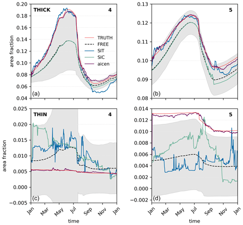
Figure 10 Category-level impact of assimilating in a thin versus thick ice state. The model's two thickest area categories for the standard case (a and b; THICK) are repeated from Fig. 8. A corresponding experiment in which mechanical ridging is restricted (c and d; THIN), leading to very low concentrations of ice in the thickest ITD categories, is also shown. These results demonstrate that the strength of the relationship between SIT observations and modeled A_ice,n breaks down when some categories have very little ice and that this can bias the modeled SIC result.

There also appears to be evidence that assimilating categorized observations may consistently constrain the sea ice state across various mean state grid cell thicknesses. In Fig. 8, assimilating SIT observations and categorized area observations perform comparably to constrain a categorized sea ice state that is relatively thick and thus has a non-negligible amount of ice in each category, including the thickest. By comparison, Fig. 10c and d present a case in which the dynamics forcing is withheld from the model integration, thereby preventing the buildup of ice in the thickest two ice categories via mechanical processes (i.e., ridging). In all other respects, the model configuration is identical to previous experiments. This leads to an overall thinner mean state in which SIT observations fail to constrain the thick ice categories. While the erroneous adjustments made in the thickest two ice categories during assimilation are relatively minimal compared with the total grid cell mean SIT (note the y axes in Fig. 10), we observe that they lead to noticeable low biases in modeled SIC (not shown). Assimilating categorized area observations appears to avoid this issue entirely (Fig. 10c, d) – the modeled quantities produced by doing so are consistent with TRUTH in all categories and total SIC.

At least two potential applications of this result in more realistic experiments exist. First, in more practical applications, the assimilation of categorized variables may avoid introducing small errors in low-concentration ITD categories that occur when assimilating SIT. This has the potential to mitigate the overall error propagation of the model during intervals in which real-world SIT observations are historically unavailable to constrain the state (i.e., during summer months). Second, it has been noted in previous work that assimilating SIT can lead to biases in the sea ice edge (Riedel and Anderson, 2024), which introduces an incentive to assimilate SIC as well as SIT, despite the negative impact that SIC can have on modeled quantities away from the ice edge. The consistency resulting from assimilating categorized observations in multiple ice states, including regimes in which the ice state is skewed to one end of the ITD, suggests a better solution for constraining the sea ice state everywhere in the Arctic.

4 Discussion

This work reinforces the results of previous studies that assimilating SIT observations generally improves sea ice analyses over assimilating SIC observations alone. In these experiments, assimilating SIT followed by SIC leads to comparable but slightly degraded modeled quantities when compared to just assimilating SIT, which implies that, for this ensemble and mean state, there is very little benefit to assimilating SIC observations, especially outside the boreal summer season. This finding, which applies to SIC analyses as well as SIT, may be due, in part, to the fact that we have generated spread in our ensemble using only variable atmospheric forcing and that the ensemble is under-dispersive with respect to SIC for much of the year. It is worth noting, however, that assimilating SIT still improves modeled SIC in this under-dispersive SIC scenario.

An emergent finding of this work is the positive impact of assimilating the categorized state (the ITD). Assimilating categorized area and volume estimates reduces the MAE and increases the CE on par with assimilating SIT observations, improving the model's estimates of SIC and SIT at the category level, even when some categories contain very little ice. Assimilating categorized observations also reduces the forecast error beyond that of assimilating aggregate observations (Figs. 4, 8), although this is likely related at least to the fact that the categorized observation errors can be quite small (see Sect. 2).

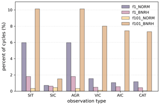
Figure 11 Percentage of DA cycles requiring SIC post-processing. For each type of observation assimilated with the four filters (f1_NORM, f1_BNRH, f101_NORM, or f101_BNRH), the percentage of total DA cycles over the course of each experiment that resulted in nonphysical values of aggregate SIC is shown. Note that the percentage of post-processing when assimilating SIC is artificially small, as those observations do not lead to substantial adjustments from the FREE mean except in the summertime, when the grid cell aggregate SIC is decidedly lower than the upper bound (no post-processing occurs during this time).

The application of a series of bounded filtering algorithms is novel to sea ice data assimilation and has highlighted the complexities of assimilating observations into a categorized distribution model such as CICE-SCM. The sometimes negligible or even detrimental impact of bounded algorithms on modeled sea ice quantities indicates a need to further tailor the CICE-SCM-DART interface such that the filters constrain categorized variables and SIC simultaneously. Bounded algorithms eliminate any need for post-processing of V_ice,n, SIT, or V_sno,n (not shown). However, for modeled SIC, we find that bounded algorithms result in a small fraction of the adjustments made requiring SIC post-processing (Fig. 11). Note that assimilating categorized observations reduces post-processing requirements compared with assimilating aggregate observations, likely because the categorized observations are closer in nature to the model's state variables.

While the broad strokes of these results are expected to carry over to assimilating real-world observations, the details are likely to vary under replication in larger models, where dynamic exchange between grid cells imbues additional information into the observation–state relationships and introduces the need for localization in the data assimilation framework. We also acknowledge that the bounded filtering algorithms employed in this work depend on piecewise distributions that are a function of the model ensemble and are relatively uninformed otherwise. DART provides the opportunity to use alternative distributions that may qualitatively shift the results. Finally, the work presented here avoids the role of various forms of model error that are present in operational data assimilation, where the observations and evolution between them are unlikely to be correctly captured by forward operators and model physics. Therefore, at the very least, the magnitude of error reductions in sea ice analyses presented may overestimate what will be achievable in more practical applications.

5 Conclusions

We have interrogated, in detail, the grid-cell-level response of a complex sea ice model to the assimilation of various kinds of sea ice observations, including SIT, SIC, and categorized area and volume, and found that SIT and categorized observations most accurately constrain the ensemble mean forecast in both category ITD state variables and diagnostic grid cell mean SIT and SIC; categorized observations are the only observations that perform consistently well across two different grid cell mean thickness states. Two key issues in the application of bounded data assimilation algorithms to the sea ice problem are identified. First, an approach to appropriately constrain categorized area and total SIC simultaneously is still needed. Secondly, a true understanding of where and why assimilation improves (or degrades) model estimates of the sea ice state depends on how well the model ensemble captures natural covariance relationships between observables and state variables on a grid cell scale. Quantification of these relationships requires a targeted study, which is absent from previous literature. Although observational records are short, we believe that significant progress could be made in understanding the local covariance relationships between SIC and SIT with current in situ and remote-sensing products. Future work will attempt to address the first issue and diagnose the second. Assuming that the ensemble is reasonably realistic in terms of the relationship between variables, the findings presented here are expected to be qualitatively consistent in larger grid models and more practical assimilation experiments.

Appendix A

Figure A1 RMSE reduction as a function of filter type and observation kind. Same as Fig. 6 but for percent RMSE reduction (pRMSE).