Characterization of non-Gaussianity in the snow distributions of various landscapes

Seasonal snowpack is an important predictor of the water resources available in the following spring and early-summer melt season. Total basin snow water equivalent (SWE) estimation usually requires a form of statistical analysis that is implicitly built upon the Gaussian framework. However, it is important to characterize the non-Gaussian properties of snow distribution for accurate large-scale SWE estimation based on remotely sensed or sparse ground-based observations. This study quantified non-Gaussianity using sample negentropy; the Kullback–Leibler divergence from the Gaussian distribution for field-observed snow depth data from the North Slope, Alaska; and three representative SWE distributions in the western USA from the Airborne Snow Observatory (ASO). Snowdrifts around lakeshore cliffs and deep gullies can bring moderate non-Gaussianity in the open, lowland tundra of North Slope, Alaska, while the ASO dataset suggests that subalpine forests may effectively suppress the non-Gaussianity of snow distribution. Thus, non-Gaussianity is found in areas with partial snow cover and wind-induced snowdrifts around topographic breaks on slopes and on other steep terrain features. The snowpacks may be considered weakly Gaussian in coastal regions with open tundra in Alaska and alpine and subalpine terrains in the western USA if the land is completely covered by snow. The wind-induced snowdrift effect can potentially be partitioned from the observed snow spatial distribution guided by its Gaussianity.

1 Introduction

Modeling of the spatial variability in snow is important for large-scale Earth surface modeling since atmospheric circulation is sensitive to the presence of snow cover (e.g., Aas et al., 2017; Meng, 2017; Mott et al., 2015, 2017; Nitta et al., 2014; Younas et al., 2017). Since subgrid variability often causes appreciable bias in weather predictions (e.g., Lalande et al., 2023; Rudisill et al., 2024), accurate snow cover quantification can potentially improve the predictability of weather, planetary-boundary-layer evolution, convective cloud formation, and even tropical cyclogenesis (Santanello et al., 2018). Hence, the subgrid variability in snow cover has been incorporated into operational regional weather-forecasting models such as the High-Resolution Rapid Refresh (HRRR) model (He et al., 2021).

Observations of seasonal snow storage in mountainous areas through remote-sensing and ground-based measurements are a direct and reliable indicator of the water supply during the following spring season in downstream regions (e.g., Fleming et al., 2023; Sengupta et al., 2022). However, total basin snow water equivalent (SWE) estimation usually requires a statistical relationship such as the snow depletion curve (SDC), which correlates with observables such as the snow cover area fraction (SCF). Based on a study of the observed snow distributions in the Reynolds Creek experimental watershed in Idaho, Luce et al. (1999) showed that one snow distribution can reasonably represent the SDC evolution for the rest of the season. Also, Luce and Tarboton (2004) showed a high degree of similarity in 9 years of dimensionless depletion curves measured in the same basin. Shamir and Georgakakos (2007) demonstrated the consistency of SDC over a season in the American River using a distributed model. The subseasonal and interseasonal consistency in SDCs suggests the possibility for subgrid snow characterization as well as basin-wide SWE estimation from SCF data such as the MODIS product (Hall et al., 2006).

As remote-sensing technologies advance, seasonal snow distribution characterization becomes more approachable with multi-sensor methods. For example, Tarricone et al. (2023) analyzed three interferometric synthetic aperture radar (InSAR) image pairs to assess SWE evolution using the snow-focused multi-sensor method with uninhabited aerial vehicle synthetic aperture radar (UAVSAR) and L-band InSAR data, as well as gather optical fractional snow-covered area (SCA) information. However, to estimate the total basin SWE in water resource management practices, statistical empirical relationships are required to fill gaps in the spatial and temporal resolutions – even when using these remote-sensing observations (Tsang et al., 2022). For example, Meloche et al. (2022) assumed a log-normal distribution to represent the sub-pixel variability in remotely sensed data. Thus, uncertainty and subgrid variability must be accounted for when using statistical characterization in SWE estimation.

The most popular choice for the probability density function (PDF) of snow is the log-normal distribution, which inherently eliminates negative snow depth (Donald et al., 1995; Liston, 2004; and many others). Brubaker and Menoes (2001) chose a beta distribution, while Kolberg and Gottschalk (2006) selected a two-parameter γ distribution. Although these common distributions are in the exponential family, they were primarily chosen for convenience. Indeed, the representativeness of these parametric probability distributions remains questionable for different landscapes and snowpack ages (e.g., Skaugen and Randen, 2013; Egli and Jonas, 2009; He et al., 2019). Moreover, these approaches for bounded distributions may not work for evolving snowpacks with partial SCA where values of zero are present in the probability domain.

In theory, without microtopography and meteorological effects and since the landing location of each snow particle fallen from the atmosphere is considered an independent and identically distributed (IID) random variable, the resulting snow depth or SWE distribution should asymptotically approach a Gaussian distribution due to the central limit theorem. He et al. (2019) reported non-Gaussian snow distributions in open areas as well as Gaussian snow distributions in the fully snow-covered forested areas during the peak snow season using airborne light detection and ranging (lidar) observations at Snowy Range, Wyoming. This implies the presence of both systematic (non-Gaussian) and random (Gaussian) mechanisms in snow accumulation and ablation processes. Therefore, it is possible to identify the potential factors as signals that make the snow distribution deviate from a Gaussian distribution by analyzing the resultant snow distributions.

This study applies negentropy to analyze the non-Gaussianity of snow distributions in the Arctic tundra, as well as in alpine and subalpine landscapes in North America. Negentropy measures the departure in entropy between a sampled distribution and a Gaussian distribution of identical variance and mean. Signals of interest (e.g., systematic snowdrift patterns) can be extracted as non-Gaussian components because pure random noise asymptotically becomes Gaussian in theory. This is the main idea of independent component analysis (ICA; Hyvärinen et al., 2001). This work presents the quantified non-Gaussianity of the observed snow distributions through a variety of snow distribution data, including intense, direct hand measurements within 30 m grids using a probe, and indirect measurements using snow-machine-attached ground-penetrating radar (GPR), UAV-based photogrammetry, and the Airborne Snow Observatory (ASO) SWE products.

2 Methods

2.1 Negentropy

To measure the non-Gaussianity of any data, we implement the information theory metric of negentropy as the objective function since negentropy is equal to the Kullback–Leibler divergence between p_x and a Gaussian distribution with the same mean and variance as p_x. There is a well-known proposition that Gaussian density has the largest information entropy among all unbounded distributions, with the same first- and second-order statistics. As such, the non-Gaussianity of an observed distribution can be quantified by negentropy J, which is defined as follows (Hyvärinen et al., 2001):

$$\begin{array}{}\text{(1)}& J\left(X\right)=S\left(X_{\text{gauss}}\right)-S\left(X\right),\end{array}$$

where S is the information entropy of X. The information entropy can assume a diversity of metrics ranging from the most general, capturing microphysical event-scale codependence in nonlinear statistical mechanics (Perdigão, 2018), to a simple assumption of basic event-scale independence in classical information theory (Shannon, 1984, statistical entropy). For the purpose of this study, we take the latter simple form, which is defined as

$$\begin{array}{}\text{(2)}& S\left(X\right)=-\int p_x\left(\mathit{\eta }\right)\log \left[p_x\right(\mathit{\eta }\left)\right]\mathrm{d}\mathit{\eta },\end{array}$$

where p_x is the PDF of X, and η is a dummy variable for the integration. The Edgeworth expansion (Edgeworth, 1905) can provide an approximation for a PDF of X as follows:

$$\begin{array}{}\text{(3)}& {\displaystyle }\begin{array}{rl}{\displaystyle }{p}_x& {\displaystyle }\left(X\right)=\\ {\displaystyle }& {\displaystyle \frac{\mathit{\varphi }\left(U\right)}{\mathit{\sigma }}}\left[\mathrm{1}+{\displaystyle \frac{{\mathit{\kappa }}_{\mathrm{3}}}{\mathrm{6}}}{H}_{\mathrm{3}}\left(U\right)+{\displaystyle \frac{{\mathit{\kappa }}_{\mathrm{4}}}{\mathrm{24}}}{H}_{\mathrm{4}}\left(U\right)+{\displaystyle \frac{{\mathit{\kappa }}_{\mathrm{3}}^{\mathrm{2}}}{\mathrm{72}}}{H}_{\mathrm{6}}\left(U\right)+\mathrm{\dots }\right],\end{array}\end{array}$$

where U is the standardized random variable of X, H_k(U) are Chebyshev–Hermite polynomials, ϕ(U) is the standard normal density, and κ_k is the kth-order cumulant of U.

Substituting the Edgeworth series into the negentropy definition, Comon (1994) obtained the analytical expression

$$\begin{array}{}\text{(4)}& J\left(X\right)={\displaystyle \frac{\mathrm{1}}{\mathrm{12}}}{\mathit{\kappa }}_{\mathrm{3}}^{\mathrm{2}}+{\displaystyle \frac{\mathrm{1}}{\mathrm{48}}}{\mathit{\kappa }}_{\mathrm{4}}^{\mathrm{2}}+{\displaystyle \frac{\mathrm{7}}{\mathrm{48}}}{\mathit{\kappa }}_{\mathrm{3}}^{\mathrm{4}}-{\displaystyle \frac{\mathrm{1}}{\mathrm{8}}}{\mathit{\kappa }}_{\mathrm{3}}^{\mathrm{2}}{\mathit{\kappa }}_{\mathrm{4}}+O\left(n^{-\mathrm{2}}\right).\end{array}$$

This is the estimator of negentropy at the fourth-order cumulant. In practice, a more intuitive approximation is commonly used:

$$\begin{array}{}\text{(5)}& J\left(X\right)={\displaystyle \frac{\mathrm{1}}{\mathrm{12}}}\text{skew}(U{)}^{\mathrm{2}}+{\displaystyle \frac{\mathrm{1}}{\mathrm{48}}}\text{kurt}(U{)}^{\mathrm{2}},\end{array}$$

where skew and kurt are the skewness and kurtosis of the standardized variable, U, respectively.

The sample estimation of the higher-order moment and cumulant (e.g., skew and kurtosis coefficients) is known to be sensitive to the presence of outliers. In this study, the interquartile range (IQR) method was adopted for outlier removal, with a minimum removal that lies outside the range of 3 times the IQR.

While negentropy metrics and the corresponding Edgeworth approximations have previously been explored and further developed in atmospheric sciences and in physics, including derivations and implementations to higher-order distributions and elaborate numerical and analytical estimators (Pires and Perdigão, 2007; Perdigão, 2010, 2017), the present study brings a simplified treatment not yet explored in hydrology that is made for swift and seamless integration within hydrological and water resource system investigations.

2.2 Data collection

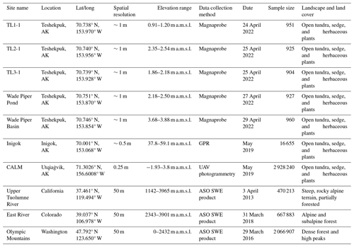
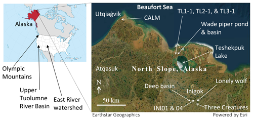
We analyzed four types of data with different collection methodologies at various scales in this study, as listed in Table 1. The first is manual snow depth surveys using a GPS-aided snow probe (Magnaprobe; Sturm and Holmgren, 2018), the second is snow depth transects using a snow-machine-attached GPR, the third is snow depth maps using UAV-based photogrammetry, and the last is the SWE product of the ASO. The first three datasets are for the open tundra in the Arctic Coastal Plain (ACP) of Alaska, while the ASO data are for the alpine and subalpine regions of the continental USA. Detailed data specifications associated with the collection methodologies will be presented in the Results section below. Figure 1 displays the map of the snow depth surveys in North Slope, Alaska, USA.

Table 1 List of snow datasets.

Figure 1 Map of the snow survey locations in Alaska, USA, and the selected ASO sites.

3 Results

3.1 Manual snow surveys at Teshekpuk, North Slope, Alaska (May 2022)

Snow depth data were collected using a Magnaprobe (Sturm and Holmgren, 2018) in five 30 m×30 m grids with 1 m grid spacing north of Teshekpuk Lake, North Slope, AK, in May 2022. The GPS location of each measurement was automatically recorded. Figure 2 presents the interpolated snow depth distributions and corresponding histograms (right columns) in five areas near Teshekpuk. The observer measured the point scale snow depth at approximately every 1 m along a line toward flags placed 1 m apart on the surface. Since the data points were selected from undisturbed snow, the locations are unevenly distributed despite the snowpacks generally being highly hardened by wind. The relative spatial locations are considered accurate since the operator stood on the same side of the probe and followed pre-marked lines based on the tape measure; however, the absolute plotted coordinates in the figures may not be trustworthy due to the GPS horizontal accuracy of <3 m. The topography of these grids in the ACP is very flat, with elevation variation of less than 1 m, while accurate absolute elevation data are hard to compare due to the spatial inaccuracy of the Magnaprobe.

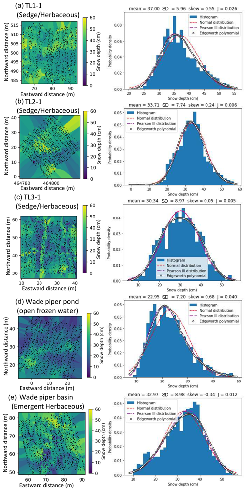
Figure 2 Manual snow distributions in the Teshekpuk Lake area, North Slope, Alaska (May 2022), and corresponding histograms with fitted probability density functions (PDFs). J denotes the computed negentropy. Snow depth histograms in open tundra in 30 m×30 m squares are generally categorized as weakly non-Gaussian. The approximated center coordinates of the grids are 70.738° N, 153.970° W (TL1-1); 70.740° N, 153.956° W (TL2-1); 70.739° N, 153.928° W (TL3-1); 70.751° N, 153.870° W (Wade Piper Pond); and 70.746° N, 153.854° W (Wade Piper Basin).

The graphics in the left column of Fig. 2 present the point depth observation locations and interpolated snow depth distributions using the nearest-distance method. The number of data points denoted by the black dots is n=951 (TL1-1), n=925 (TL2-1), n=904 (TL3-1), n=927 (Wade Piper Pond), and n=960 (Wade Piper Basin).

The corresponding snow depth histograms and three fitted distributions are displayed in the right column. The statistical mean, standard deviation, skew coefficient, and negentropy (J) are reported at the top of each graph. In general, the snow depth distributions in these areas are almost Gaussian distributions since the computed negentropy is small. However, the negentropy of the snow distribution affected by wind-induced snowdrift (sastrugi) on frozen lakes is larger than the tundra covered by sedge and herbaceous vegetation. In practice, the non-Gaussianity of seasonal snow depth may have been negligible in the coastal open tundra (including frozen open waters) in the Teshekpuk study area in May 2022.

3.2 Snow depth surveys using GPR along multiple transects in Inigok, North Slope, AK (April 2019)

The Inigok area of North Slope, Alaska (70.001° N, 153.068° W) is characterized by paleo-sand dunes (Carter, 1981), hydro-geomorphological processes, and permafrost landforms such as thermokarst lake formation and drainage. The landscape is characterized by relatively steep terrain and substantial wind-induced snowdrifts (deeper than 5 m), especially around lake shores and drainage channels (e.g., Rangel et al., 2023a).

Snow depth surveys using a GPR are particularly effective for deep-snow areas since the Magnaprobe is only 1.5 m long. Considering the lower limit of the selected GPR antenna, we collected several GPR transects (Malå ProEx, 800 MHz, GuidelineGeo, Sundbyberg, Sweden) around Inigok, where the snowpack was deeper than in the coastal area. The antenna was placed on a sled towed by a snow machine traveling <5 km h⁻¹. The effect of compaction by the snow machine was considered negligible because the snow was highly wind-packed and therefore was not affected by the weight of the snow machine during data collection. The GPR data were processed in ReflexW (Sandmeier Software, Karlsruhe, Germany) using a low-frequency-noise removal (dewow) and a linear gain with topographic correction adapted from the ArcticDEM (Rangel et al., 2023b). Maps of snow depth estimated from the GPR transects are shown in Fig. 3. The line color denotes the observed snow depth (the darker, the deeper). A substantial snowdrift developed near the lakeshore's banks due to its steep topography.

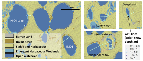
Figure 3 Snow depth surveys using GPR along multiple transects in Inigok, North Slope, Alaska (27 and 28 April 2019), superimposed over the land cover map with 1 m interval contour lines. The approximated center coordinates of the maps are 70.005° N, 153.105° W (INI04 and INI01); 69.993° N, 152.949° W (Lonely Wolf); 69.992° N, 153.274° W (Deep Basin); and 69.942° N, 153.032° W (Three Creatures and Independent Fox).

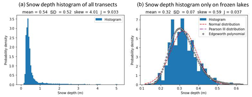
Figure 4 displays the histograms of GPR snow depth data in Inigok, North Slope, Alaska, in May 2019 when using (panel a) all transect data and (panel b) the frozen lake sections only. The snow depth histogram of all transects shows strong non-Gaussianity due to a mix of steep and flat terrain. However, the histogram of the partial dataset for only the frozen lakes shows much weaker non-Gaussianity. In fact, snow distribution after removing the deep-snow parts can be reasonably approximated by the Gaussian distribution with a negentropy of 0.037, which is the same level as Wade Piper Pond (Fig. 2) in the previous section (J=0.040). Therefore, the snowdrift due to steep terrain is considered a major source of non-Gaussianity in snow depth in open tundra.

Figure 4 Snow depth histograms of GPR snow survey data from Inigok, North Slope, Alaska (April 2019), using (a) all transects and (b) sections on frozen lakes only. Snow distributions in the Inigok area are highly non-Gaussian, while the frozen lake subset shows weak non-Gaussianity.

3.3 Snow depth distribution based on UAV footage of a drained lake basin within the CALM 1 km grid near Utqiaġvik, AK (May 2019)

Figure 5 (left panel) presents the observed snow distribution of a drained thermokarst lake basin referred to as Central Marsh, part of the Circumpolar Active Layer Monitoring (CALM) network located east of Utqiaġvik, Alaska. The snow depth was estimated by differentiating the snow surface elevation and the snow-free ground elevation using UAV surveys with the photogrammetry technique. The images were collected on 4 August 2019 (snow-free) and 15 April 2019 (snow-covered), using a Phantom 4 UAV (P4RTK). Images were post-processed/georeferenced to NAD83 zone 4 north in ellipsoid heights using a propeller AeroPoint and Pix4D (version 4.3.33 for the April survey, 4.4.12 for the August survey) at a 0.25 m spatial resolution (Nichols, 2020). The vertical accuracies of these measurements are 18 and 10 cm for the April and August surveys, respectively. The horizontal resolution for the snow depth is 1 m.

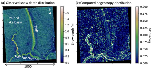
Figure 5 The snow depth distribution based on UAV photogrammetry and the computed negentropy distribution of 30 m moving windows in a drained lake basin in the CALM 1 km grid (71.3026° N, 156.6008° W) near Utqiaġvik, Alaska.

The CALM site is situated in the ACP in northern Alaska, which has typical complex terrain due to the recently drained thermokarst lake with sparse or negligible vegetation and well-developed polygons. There is an obvious smoothed bluff in the center of the domain, and the west side of this bluff tapers into the drained lake basin. The incised drainage channels cause steep land features that capture sizable snowdrifts in the southern part. In the southern portion of the area, the polygons are formed by ground-surface cracks with ice wedge development beneath found in the lower and higher center parts in the left panel of Fig. 5.

The negentropy distribution in the moving window may be obtained from these gridded snow data at a very high spatial resolution. The right panel of Fig. 5 presents the computed negentropy map in the CALM area with a 30 m moving window. Overall, non-Gaussianity at the CALM site was found to be weak – even with the smoothed bluff and despite high snow depth. However, as whiter parts in right panel of Fig. 5 are found along the drainage channels, topographic discontinuity around the incised gully seems to cause significant non-Gaussianity. Additionally, vegetation patches may cause spotty non-Gaussianity in the northern part of the area. Conversely, since the southern parts covered by the polygons show a darker color (J<0.025), except the drainage channels, the ground-surface polygon does not make snow distribution non-Gaussian. Overall, snowpack in the coastal parts of the ACP can be reasonably approximated by a Gaussian distribution since most of the CALM area showed low negentropy of less than 0.2.

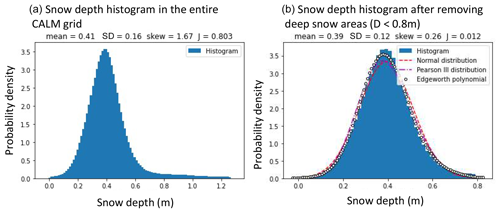
Figure 6 presents the snow depth histogram, which looks like a Gaussian distribution with a long tail due to snowdrift around the gullies in the CALM grid. In fact, when the deep snowdrifts of the gully and the bluff are removed from the samples, the histogram more closely resembles a Gaussian distribution (see the right panel in Fig. 6).

Figure 6 Snow depth histograms based on the UAV photogrammetry of a drained lake basin in the CALM 1 km grid near Utqiaġvik, Alaska. Removing the deep snow caused by wind-induced snowdrift results in a near-perfect fit by a Gaussian distribution.

3.4 SWE products based on ASO data for the selected watersheds

SWE is a stable and direct indicator of snow/water distribution in landscapes. As such, the SWE products from the Airborne Snow Observatory (ASO) were selected (Painter et al., 2016) to examine the Gaussianity of snow distributions in different climate zones and landscapes with alpine-to-subalpine snowpack. The snow depth and SWE distributions were estimated from the coupled imaging spectrometer and scanning lidar, then combined with distributed snow modeling (including snow density simulation). The ASO snow products are considered some of the most comprehensive instantaneous snow distribution estimations at a fine resolution (50 m). We used the processed snow product to characterize the medium-scale snow distribution with the same outlier treatment (IQR method) as described above.

The analysis of three representative SWE datasets in the western USA is presented. These include the upper Tuolumne River watershed in California (USCATB, 3 April 2013), the East River watershed above Gunnison, Colorado (USCOGE, 31 March 2018), and the Olympic Mountains in Washington (USWAOL, 29 March 2016).

3.4.1 Tuolumne River watershed, California

Figure 7 presents the composite graphics of the data and the analysis results for the upper Tuolumne River watershed on 3 April 2013. Panel (a) shows the SWE distribution estimated by the ASO, while panel (b) visualizes the normalized SWE histogram or PDF within the entire domain with the fitted theoretical distributions. Panels (c) and (d) are the negentropy distributions of the SWE within 1500 m moving windows with and without partially snow-covered cells. Panel (e) shows the National Land Cover Database (NLCD) 2011 land cover map for reference. The watershed (1175 km²) is one of the drainages to California's Central Valley through the Hetch Hetchy Reservoir in the southern Sierra Nevada mountain range. The boundary of the catchment is mostly comprised of steep, rocky, alpine terrain (which contributes to the attractive land features of Yosemite National Park), whereas the bottom of the valley is relatively flat due to past glacial processes. The snow distribution (panel a) shows a clear relationship with elevation, while the SWE barely exceeded 1 m during the observation period in peak snow season. The overall SWE histogram (panel b) illustrates strong non-Gaussianity because of snow-free and shallow accumulation areas in the watershed (bounded distribution effect).

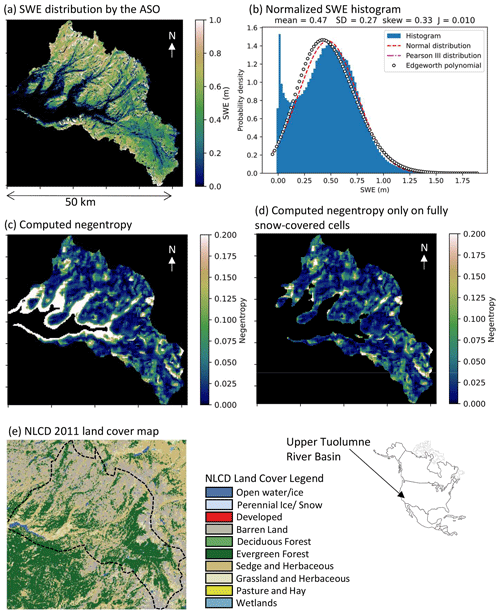
Figure 7 (a) SWE distribution based on ASO data from the upper Tuolumne River basin, California, USA, from 3 April 2013 (USCATB; 37.461° N, 119.494° W); (b) normalized SWE histogram; (c) negentropy map of the SWE within 1500 m moving windows; (d) negentropy map of only fully snow-covered cells; and (e) NLCD 2011 land cover map.

However, the local negentropy map with moving windows (panel c) shows low non-Gaussianity except in the low-elevation areas. In fact, the majority of high non-Gaussianity cells are from partially snow-covered cells. When the partially snow-covered cells are removed in panel (d), the local negentropy falls by less than 0.15 in most of the watershed. Therefore, the bounded distribution effect in the probability domain from the partially snow-covered cells brings substantial non-Gaussianity into the snow distribution.

Additionally, the spatial resolution of 50 m may be too coarse to capture the local snowdrift effect discussed in Sect. 3.2 and 3.3 using the very-fine-resolution data since snowdrift extent around steep cliff is often smaller than the resolution of medium-to-large-scale snow products. Therefore, even with fully snow-covered areas, fine-resolution data are required for snowdrift characterization, which is potentially important for more accurate snow storage estimation. However, further study is recommended using finer-resolution snow data, although the combined effect of steep terrain and vegetation on snowdrift is highly complicated and hard to characterize even with modern remote-sensing technology.

3.4.2 East River, Colorado

The ASO dataset of the East River above Gunnison, Colorado (USCOGE), was selected as a representative basin in the Rocky Mountain region. This dataset includes the US Department of Energy (DOE) East River community observatory, where comprehensive field data have recently been collected (Kakalia et al., 2021). The data domain, which does not agree with the watershed boundary, is approximately 1670 km², with the elevation ranging from 2343 m (Gunnison) to 3901 m. Figure 8 displays the corresponding analysis results of the East River area on 31 March 2018.

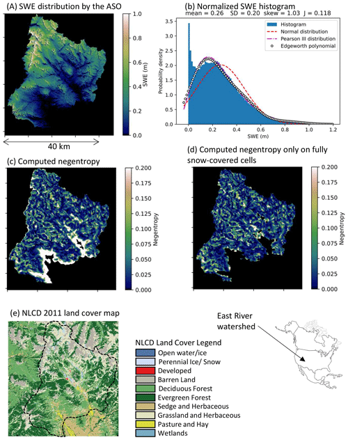
Figure 8 (a) SWE distribution based on ASO data for the East River watershed above Gunnison, Colorado, USA, from 31 March 2018 (USCOGE; 39.037° N 106.978° W); (b) normalized SWE histogram; (c) negentropy map of the SWE within 1500 m moving windows; (d) negentropy map of only fully snow-covered cells; and (e) NLCD 2011 land cover map.

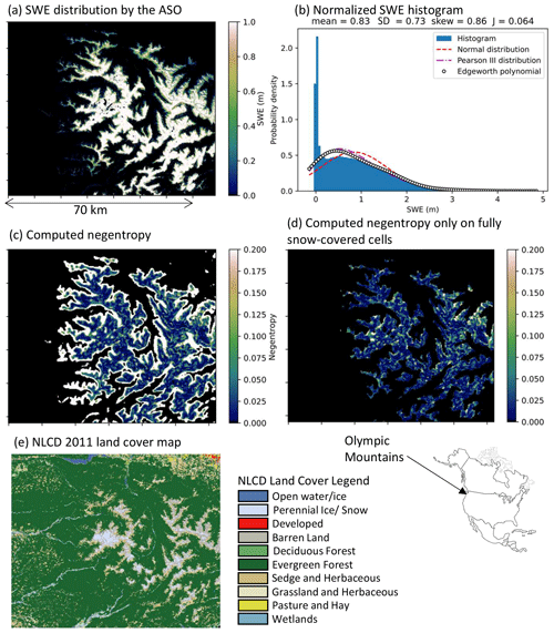
Figure 9 (a) SWE distribution based on ASO data for the Olympic Mountains, Washington, USA, from 29 March 2016 (USWAOL; 47.792° N 123.650° W); (b) normalized SWE histogram; (c) negentropy map of the SWE within 1500 m moving windows; (d) negentropy map of only fully snow-covered cells; and (e) NLCD 2011 land cover map.

Besides the obvious bounded distribution effect of partially snow-covered cells, this case study illustrates the non-Gaussianity induced by the steep topographic features around the high peaks in the Rocky Mountains. However, it is interesting that the range of negentropy remains less than 0.5 in the fully snow-covered areas in panel (d) despite the very steep topography in the East River watershed. At Inigok, for example, the landscape is flat with low-rolling hills punctuated by very abrupt, very steep bluffs that cause the large drifts. In contrast, while East River certainly has much greater total topographic relief, it does not have the same long, flat fetch area where the wind can build unimpeded nor does it have similar abrupt erosional bluffs. Also, since the lower negentropy (darker colored) parts in panel d generally agree with the evergreen and deciduous forest cover extent in the NLCD land cover map in panel (e), the subalpine forest may reduce non-Gaussianity in snow distribution. However, the general characteristics of the sample's negentropy distribution in northern Colorado are consistent with the upper Tuolumne River watershed in the Sierra Nevada mountain range.

3.4.3 Olympic Mountains, Washington

The last example of snow non-Gaussianity quantification is the Olympic Mountains in Washington, USA, which represent the northern Pacific Coast Range under a strong oceanic influence. The elevation ranges from sea level to 2430 m. The Olympic Mountains consist of a cluster of steep-sided peaks, heavily forested foothills, and incised deep valleys. The ASO data have a large spatial coverage (5330 km²) when compared to the other two ASO datasets presented here.

The black areas in the high-elevation range in panel (a) are the approximate glacier extent excluded from the analysis (Painter and Lettenmaier, 2018). A large fraction of partially snow-covered cells also introduces non-Gaussianity in SWE in this region. Meanwhile, dense evergreen forests in the Olympic Mountains seem to effectively reduce the non-Gaussianity of SWE above the snow line during the ASO scanning period. Overall the non-Gaussianity of the snowpack may be considered low when compared to the other two examples, which is likely due to denser forest cover. Presumably, the vegetation cover minimizes the wind-induced snow redistribution process and makes the snow distribution more Gaussian. These characteristics – i.e., non-Gaussianity in partially snow-covered areas and high Gaussianity in forested areas – are common features of the SWE distributions throughout the western USA.

4 Discussion

The sample negentropy values presented here are generally consistent with each other despite the variety of data collection methods used at different scales. The level of random noise in the datasets depends on the data collection methods. Among the datasets discussed here, one may anticipate that the ASO data have the largest Gaussian bias due to multiple remote sensing, resampling, assimilating, and modeling procedures covering remarkable spatial coverage with uniform data quality. The UAV-based lidar data at the North Slope CALM site are expected to have a noticeable random bias with a vertical accuracy of approximately 12 cm. The GPR snow depth observations should have a smaller but appreciable Gaussian bias due to snow quality variation and non-flat snow surface elevation (antenna angle vibration), although the continuous measurement minimizes the random relative error in the snow depth estimation. The hand-measured snow depth data using a probe may include the least Gaussian bias, while the sampling spacing was not uniform due to relatively poor spatial positioning control with the Magnaprobe's onboard GPS unit. Despite these differences, it is encouraging that the quantified Gaussian levels were comparable and consistent since they share common features.

Table 2 Summary of the analysis using the sample negentropy.

The stability of the sample estimator of negentropy may be a potential issue, especially when the sample size is small. Additionally, since the higher-order statistical moments are sensitive to the presence of outliers in the sample, an outlier removal filter is recommended for large samples. The IQR method with a threshold of 3 IQR above the third quarter (Q3), which is stricter than the usual threshold (typically 1.5 IQR), has been applied to the UAV photogrammetry data and the ASO datasets for computational stability. Even with the large threshold (small outlier removal), the proposed method using negentropy appears to be effective in characterizing the Gaussianity of snow distribution, which is a common implicit assumption for existing gridded data and models. This study visualized the limitations of such a common distribution assumption for snow distribution, specifically for areas with partial snow cover.

To summarize the analyses presented here, five categories of Gaussianity were defined and associated with a magnitude of a sample statistic value (see Table 2). Most of the fully snow-covered areas fell into the category of almost Gaussian, with negentropy less than 0.03. Notably, negentropy less than 0.01 is considered nearly perfectly Gaussian, as can be seen in the previous sections.

The Gaussianity characterization of snow distribution appears to be useful in distinguishing the snowdrift-affected areas using the sample negentropy. Simultaneously, this finding can justify the implicit Gaussian assumption for snow distribution for overall SWE estimation, particularly for snowpack characterization from remotely sensed information. For instance, the effect of higher-order statistical moments can be negligible in most fully snow-covered areas. Conversely, some additional statistical treatment for higher-order statistics may be required for the areas with the non-Gaussian effects around snow lines, open wind-swept areas, and sharp terrain. Additionally, since a consistent pattern in the skew coefficient was not identified from the snow datasets, the commonly used log-normal distribution may not be suitable for those areas.

It is encouraging that snow depth and SWE distributions are generally approximated well by the Gaussian or weakly non-Gaussian distribution, which is a fundamental assumption for statistical characterization of the subgrid variability used in snowpack estimation by remote sensing. The non-Gaussianity found in the partially snow-covered areas can also be modeled by a truncated normal distribution, although it must be tested further. Moreover, the weakly non-Gaussian distribution would enable the Edgeworth expansion method proposed by Pires and Perdigão (2007). For instance, the non-Gaussian asymptotic method or information metric can effectively determine the saddle point approximation of the joint probability density functions (PDFs) through maximizing the Shannon entropy between the remotely sensed signal and the SWE. Thus, the quantification of non-Gaussianity in snow depth/SWE distributions would be an important milestone toward accurate snow water quantification using remote-sensing techniques as well as grid-based snow and Earth surface models.

5 Conclusions

A Gaussian snow distribution is a common underlying assumption for finite-scale models or gridded datasets. The present study tested this assumption using the sample negentropy of various snow data. We found two main sources of non-Gaussianity: (1) a partial snow cover effect (bounded distribution) and (2) a wind-induced snowdrift effect around steep terrain features. The second effect may amplify the first one in wind-swept alpine areas since snow erosion remains shallow on rocky ridges and peaks. Snowdrift around lakeshore cliffs and deep gullies can bring moderate non-Gaussianity on the open tundra of North Slope, Alaska. However, the wind-packed snow in the coastal plain region of the North Slope may generally be categorized as weakly Gaussian during mid-to-late winter due to the continuous snow cover. This implies that the non-Gaussianity of the snowpack should not be neglected during the snow accumulation season and late-spring season. Interestingly, small ground-surface features (e.g., low-centered and high-centered ice wedge polygons) make snow distribution more Gaussian, while snowdrifts (snow dunes) on a flat frozen lake seem to be less Gaussian than on tundra or in a drained lake basin.

Our analyses of the ASO SWE products reinforced the findings for snowpacks on the tundra. Although SWE data were chosen instead of snow depth for practical reasons, the common features of non-Gaussianity remain valid. Additionally, the snow diffuser effect of forests was illustrated in three representative areas in the western USA. This effect was reported by He et al. (2019) based on airborne lidar snow depth measurements at Snowy Range, Wyoming, USA. Hence, it is likely that vegetation cover generally makes the snow distribution more Gaussian during the snow accumulation process; however, further verification of this relationship is recommended.

Overall, a Gaussian distribution is a suitable approximation for snow spatial distribution when the ground is completely covered by snow. Higher-order statistics associated with landscape type may potentially improve the SWE estimation in windswept open terrain and near snow lines. The level of non-Gaussianity will determine the choice of statistical tool to correct the systematic bias in the snow measurements. Meanwhile, this study suggests the possibility of partitioning the extent of wind-induced snowdrifts by means of independent component analysis (Comon and Jutten, 2010).