the Creative Commons Attribution 4.0 License.
the Creative Commons Attribution 4.0 License.
 | 06 Feb 2024
Improved monitoring of subglacial lake activity in Greenland
Louise Sandberg Sørensen
Rasmus Bahbah
Sebastian B. Simonsen
Natalia Havelund Andersen
Jade Bowling
Noel Gourmelen
Alex Horton
Nanna B. Karlsson
Amber Leeson
Jennifer Maddalena
Malcolm McMillan
Anne Solgaard
Birgit Wessel
Subglacial lakes form beneath ice sheets and ice caps if water is available and if bedrock and surface topography are able to retain the water. On a regional scale, the lakes modulate the timing and rate of freshwater flow through the subglacial system to the ocean by acting as reservoirs. More than 100 hydrologically active subglacial lakes that drain and recharge periodically have been documented under the Antarctic Ice Sheet, while only approximately 20 active lakes have been identified in Greenland. Active lakes may be identified by local changes in ice topography caused by the drainage or recharge of the lake beneath the ice. The small size of the Greenlandic subglacial lakes puts additional demands on mapping capabilities to resolve the evolving surface topography in sufficient detail to record their temporal behaviour. Here, we explore the potential for using CryoSat-2 swath-processed data, together with TanDEM-X digital elevation models, to improve the monitoring capabilities of active subglacial lakes in Greenland. We focus on four subglacial lakes previously described in the literature and combine the data with ArcticDEMs to obtain improved measurements of the evolution of these four lakes. We find that with careful tuning of the swath processor and filtering of the output data, the inclusion of these data, together with the TanDEM-X data, provides important information on lake activity, documenting, for example, that the ice surface collapse basin on Flade Isblink Ice Cap was 50 % (30 m) deeper than previously recorded. We also present evidence of a new, active subglacial lake in southwestern Greenland, which is located close to an already known lake. Both lakes probably drained within 1 month in the summer of 2012, which suggests either that they are hydrologically connected or that the drainages were independently triggered by extensive surface melt. If the hydrological connection is confirmed, this would to our knowledge be the first indication of hydrologically connected subglacial lakes in Greenland.
- Article
(16337 KB) - Full-text XML
- BibTeX
- EndNote


A subglacial lake is a body of water stored beneath an ice sheet, ice cap, or glacier. Subglacial lakes are part of the basal hydrology and drainage system and may act as buffers between the melt generated on and below the ice and the flux to the ocean (Fricker et al., 2007; Siegert et al., 2016). The origin of the water contained in a subglacial lake depends on its regional setting. The water that feeds subglacial lakes may be generated by ice melting caused by geothermal heat or by frictional heat from ice flow or surface water channelled to the bed (Karlsson et al., 2021).
The number of observed subglacial lakes is growing (Livingstone et al., 2022; Fan et al., 2023), and while their total volume is not large, mapping their dynamics is important to better understand the movement of meltwater through the subglacial system. Currently, less than 100 subglacial lakes have been discovered in Greenland, while 675 have been detected in Antarctica (Livingstone et al., 2022). The Greenland Ice Sheet (GrIS) is warmer, thinner, and generally characterized by a steeper ice surface slope than the Antarctic Ice Sheet (AIS), and it is possible that past subglacial lakes in Greenland drained at the end of the last glacial period (Pattyn, 2008). Furthermore, subglacial lakes in Greenland are typically small and located close to the margin of the ice sheet (Bowling et al., 2019), where the rapidly evolving surface mass balance hinders the detection of subglacial lake activity.
In accordance with Livingstone et al. (2022), we define a subglacial lake as stable if its volume remains relatively constant over time or as being active if it is observed to periodically drain and refill. The lake will eventually drain when filled with enough water to overcome the pressure exerted by the overlying glacial load (Chandler et al., 2013); hence, a subglacial lake drainage event can be triggered by a prolonged addition of surface meltwater (Livingstone et al., 2022). The sudden drainage and outburst flood of a subglacial lake might temporarily affect ice flow velocities downstream from the lake location as documented by Magnússon et al. (2007), Liang et al. (2022), and Stearns et al. (2008). This is not always the case, as shown by Smith et al. (2017), where a drainage event under Thwaites Glacier in West Antarctica had no apparent impact on the ice velocities. Therefore, the behaviour of subglacial lakes is important to consider when discussing the response of the ice sheets to a warming climate (Willis et al., 2015). The behaviour of active subglacial lakes is also an important indicator of hidden subglacial processes. In particular, the period of lake recharge provides information about subglacial water production, transfer of water from surface to the bed, and conditions at the bed (Malczyk et al., 2020).
Active subglacial lakes may be identified by ice surface collapse basins (surface depressions) created when a lake drains and localized surface uplift as the lake refills. The surface expressions of subglacial lake volume oscillations are controlled by viscous ice flow (Stubblefield et al., 2021). In contrast, stable subglacial lakes are typically identified using radio-echo sounding (RES). Evans and Smith (1970) were the first to detect a subglacial lake under the AIS by RES. RES can penetrate the ice sheet and map the bedrock topography, where a strong, flat reflection indicates the presence of basal water (Bingham and Siegert, 2007; Tulaczyk and Foley, 2020). RES has been used to detect and map numerous subglacial lakes under the ice sheets (Wright and Siegert, 2012; Siegert et al., 2016; Bowling et al., 2019). Stable subglacial lakes cannot be identified from the characteristics of the overlying ice surface except for large lakes which may influence surface topography, as seen at Lake Vostok, AIS, where the surface relief is exceptionally flat (Ridley et al., 1993).
In a recent study, Fan et al. (2023) identify 18 active subglacial lakes in Greenland from surface variability based on ICESat-2 data. Prior to the Fan et al. (2023) study only four of the known subglacial lakes in Greenland had been identified by ice surface collapse basins, while the rest were identified by the use of RES (Bowling et al., 2019).
The small size of the subglacial lakes in Greenland (<1 km2) makes them impossible to map from conventionally processed radar satellite altimetry (Meloni et al., 2020), whereas their large Antarctic counterparts (10–100 km2) have been monitored extensively (Livingstone et al., 2022). However, due to the novel synthetic aperture radar interferometric (SARIn) mode of the European Space Agency's (ESA) first Earth explorer mission CryoSat-2 (CS2) and recent advances in so-called swath processing (Gray et al., 2013; Foresta et al., 2016; Gourmelen et al., 2018a; Andersen et al., 2021), even smaller targets can now be monitored, as suggested by Wingham et al. (2006). The swath processing enables us to generate a swath of elevation estimates across track, which increases the spatial data resolution and coverage. This processing method means that the ability to map topographic lows is improved compared to conventional retracking, which preferably tracks the point of closest approach (topographic highs), thus increasing the possibility of acquiring data over small surface features. An additional source of high-resolution ice surface topographic information is provided by two digital elevation models (DEMs): DEMs derived from the X-band interferometric synthetic aperture radar (InSAR) satellite mission (TanDEM-X) (Rizzoli et al., 2017) and DEMs from the panchromatic band WorldView satellite mission (ArcticDEM) (Porter et al., 2018). Here, we investigate the capabilities and added value of the CS2 swath-processed altimetry data and high-resolution TanDEM-X DEMs, focusing on four active subglacial lakes in Greenland that have previously been identified and described in the literature (Palmer et al., 2013, 2015; Howat et al., 2015; Bowling et al., 2019) since this allows us to evaluate our results. These four subglacial lakes are all characterized by the occurrence of collapse basins in the ice sheet and ice cap surface topography after a lake drainage event. Through analysis of swath-processed CS2 data, TanDEM-X DEM scenes, and ArcticDEMs, we present time series of collapse basin depths at an unprecedented temporal resolution, thus advancing understanding of the subglacial lake draining and refilling timing and rates of the four active subglacial lakes. We do not include ICESat-2 data satellite laser altimetry in this study as the main goal has been to densify the time series covered by the CS2 mission, but we acknowledge that this sensor provides an obvious data set for future monitoring of subglacial lake activity (Fan et al., 2023).
The four active subglacial lakes in Greenland that we will investigate here are all identified by observations of surface collapse basins and are located as follows: one in West Greenland, two in southwestern Greenland, and one under the Flade Isblink Ice Cap in northeastern Greenland (Fig. 1). Here we summarize the present knowledge of the lakes following Palmer et al. (2015), Willis et al. (2015), and Bowling et al. (2019). We do not include the three known subglacial lakes located beneath the Isunnguata Sermia glacier in this study due to their location in the highly dynamic region very close to the ice sheet margin (Livingstone et al., 2019).
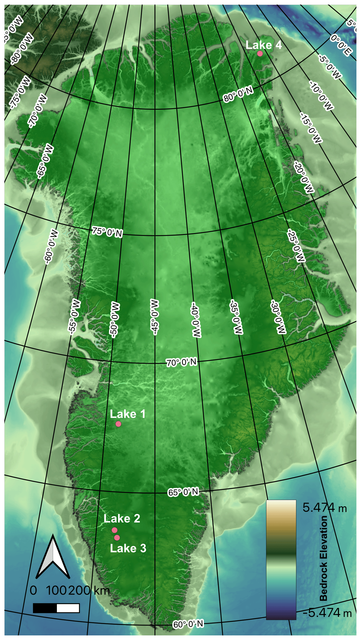
Figure 1The locations of the four sites of active subglacial lakes investigated in this study shown in a background image of bedrock elevation from BedMachine v3 (Morlighem et al., 2017).
2.1 Lake 1: West Greenland
Lake 1 is a subglacial lake located in the western part of the GrIS (67.611∘ N, 48.709∘ W) northwest of the Inuppaat Quuat glacier, just below the equilibrium line altitude (ELA). Its location and regional setting are shown in Fig. 7a using a Landsat-8 image from 2019 as background. The temporal evolution of Lake 1 has previously been studied by Palmer et al. (2015) and Howat et al. (2015), using a variety of elevation data sets such as Surface Extraction from TIN-based Search-space Minimization (SETSM) DEMs derived from WorldView data, the Greenland Mapping Project (GIMP) DEM, ICESat along-track elevations, airborne lidar data, and optical imagery. The data sets constrained the spatiotemporal evolution of the lake drainage and the associated ice surface collapse. These studies find that Lake 1 drained both in 2004 (smaller event) and in 2011 (larger event). The 2011 drainage occurred at an unknown rate within 2 weeks (28 June to 12 July 2011), resulting in the formation of a collapse basin in the ice sheet surface. A SETSM DEM from 28 October 2011 revealed a collapse basin of about 1 km in width and 60–70 m in depth. The bottom of the collapse basin was flat, which suggested that the subglacial lake was still partially filled. According to both Palmer et al. (2015) and Howat et al. (2015), it is likely that Lake 1 receives meltwater from the surface and that the drainage of Lake 1 in 2011 may have been triggered by the drainage of a nearby supraglacial lake. The routing of water to the bedrock from the surface, e.g. through a moulin, has been known to trigger drainage of subglacial lakes due to overfilling by meltwater (Willis et al., 2015). The collapse basin was observed to partially refill between 2011 and 2013; however, it could not be concluded whether the subglacial lake recharged or if the depression simply filled up with surface water or snow.
2.2 Lakes 2 and 3: southwestern Greenland
Two collapse basins are found in southwestern Greenland between the Sermeq and Sioqqap glaciers, and according to Bowling et al. (2019) these surface depressions are (with very high confidence) associated with the drainage of subglacial lakes. We denote the northernmost lake as Lake 2 (63.542∘ N, 48.449∘ W) and the southern one as Lake 3 (63.261∘ N, 48.207∘ W). The respective locations of the two lakes are shown in Figs. 8a and 9a. They are located about 35 km apart, and the collapse basin over Lake 2 was 15 m deep in August 2012, while the one over Lake 3 was 18 m deep in June 2012. Using ArcticDEM strips from 2015, Bowling et al. (2019) also found that both collapse basins decreased in volume in the period 2012–2015, which suggests a refilling of the subglacial lakes, and it was further estimated that the recharge of Lake 3 has been ongoing since 2001, while the timing of the drainage event for Lake 2 was not identified. Optical images show supraglacial lake drainage in the region, which could indicate some recharge of the subglacial lakes by surface water.
2.3 Lake 4: Flade Isblink Ice Cap
The collapse basin above a subglacial lake on the southern dome of Flade Isblink Ice Cap in the northern part of Greenland (see Fig. 10a) has been described by Willis et al. (2015) and Liang et al. (2022), and we denote it as Lake 4 (81.157∘ N, 16.613∘ W). Willis et al. (2015) base their analysis on DEMs from stereo satellite imagery, together with airborne lidar observations, while Liang et al. (2022) investigate the subglacial lake using ArcticDEMs and ICESat-2 altimetry data between 2012 and 2021. From MODIS optical imagery Willis et al. (2015) found that the ice surface above Lake 4 had subsided in the autumn of 2011, leaving a surface depression shaped like a mitten. The basin was estimated to have formed over a 3-week period between 16 August and 6 September 2011, and it comprises two sub-basins. The first estimate of elevation measurements was from a WorldView-1-derived DEM from May 2012 showing a maximum depth of the collapse basin of about 70 m. The elevation of the collapse basin rapidly increased by 30 m over the following 2 years due to inflow of surface water to the subglacial lake, and between August 2012 and April 2013 a topographic bulge appeared in the basin (Willis et al., 2015). Liang et al. (2022) find that the lake drained again in 2019, resulting in a 10 m elevation change.
In the following, we present the data sets and outline our processing steps.
3.1 TanDEM-X
TanDEM-X is an interferometric synthetic aperture radar system consisting of two satellites, TerraSAR-X and TanDEM-X, launched in 2007 and 2010, respectively. Its primary mission objective was the generation of a global digital elevation model, which was completed in 2016 with a spatial resolution of 0.4 arcsec (i.e. about 10–12 m) (Rizzoli et al., 2017). Here, we use TanDEM-X data acquired between the years 2010 and 2017. The InSAR data were requested via a TanDEM-X science proposal as co-registered single-look complex data, and the interferometric processing and calibration to produce interferometric DEM scenes were done by the German Aerospace Center (DLR) using the Integrated TanDEM-X Processor (ITP) and the Mosaicking and Calibration Processor (MCP) (Rizzoli et al., 2017). The ITP processed the interferometric bistatic data to interferograms and then performed phase unwrapping and geocoding (Lachaise et al., 2018; Rossi et al., 2012). The absolute vertical calibration of the uncalibrated DEM scenes was performed by MCP block adjustment. For Greenland, this procedure relied on ICESat points over rocks as vertical reference and tie points to transfer the height level to the data located further inland (Wessel et al., 2016). For each DEM scene, an individual height offset was estimated and applied (up to 10 m). The penetration of the X-band synthetic aperture radar (SAR) signal into the snow and ice surface by several metres (Rott et al., 2021; Fischer et al., 2020; Wessel et al., 2016) was maintained by the block adjustment and may therefore complicate validation and comparison with other data. However, this issue was bypassed in this study by aligning different DEMs at stable anchor points, which is described in Sect. 4.2. Figure 2 shows examples of TanDEM-X DEMs covering Lake 1 at different time steps, with Figs. 2a, b, and c from 2011, 2012, and 2016, respectively. Figure 2d shows the collapse basin in an optical image from July 2012. Figure 2e shows the elevation difference between February 2011 and April 2012, while Fig. 2f shows the elevation difference between April 2012 and December 2016.
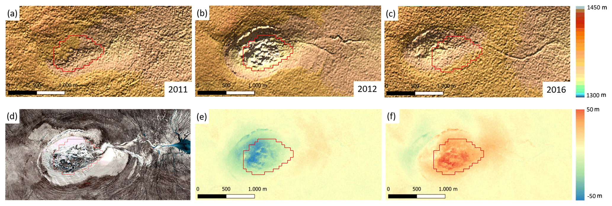
Figure 2Subset of three colour-shaded TanDEM-X DEMs for Lake 1: (a) from 17 February 2011 (before the collapse), (b) from 5 November 2012 (after the collapse), and (c) from 10 December 2016 (after some refilling). (d) WorldView optical image from 23 July 2012 (after collapse) © Google Earth. (e) Elevation difference between 4 November 2012 and 17 February 2011. (f) Elevation difference between 10 December 2016 and 4 November 2012. The outline of the core collapse basin from 2012 is displayed in red in all panels.
3.2 ArcticDEM
The ArcticDEM input data are comprised of time-stamped DEM strips with 2 m spatial resolution covering the period 2011–2017 (Porter et al., 2018). These DEMs have been generated from stereoscopic WorldView and GeoEye satellite imagery by the ArcticDEM Team, using the Surface Extraction with the SETSM algorithm (Noh and Howat, 2018). Following their generation, they are freely distributed as strip files to the community by the US Polar Geospatial Centre. The DEMs are then co-registered using lateral and vertical corrections provided within the ArcticDEM metadata (Porter et al., 2018). Examples of ArcticDEM strip data are shown in Fig. 7c for Lake 1 (October 2011), Fig. 8c for Lake 2 (July 2012), Fig. 9c for Lake 3 (May 2012), and Fig. 10c for Lake 4 (May 2012).
3.3 CryoSat-2
CS2 measures in three different operational modes: low-resolution mode (LRM), SAR mode, and SARIn mode, of which the latter can be used for swath processing (Wingham et al., 2006). Here, we swath process the CS2 SARIn Level 1b (L1b) Baseline-D data (Meloni et al., 2020). The conventional SARIn Level 2 (L2) elevation product from CS2 consists of a single surface elevation measurement at the point of closest approach (POCA) along the satellite flight line. This L2 elevation product only takes advantage of a fraction of the information contained in the 1024 measurements contained within a single CS2 waveform. By implementing swath processing of radar altimetry, it is possible to generate additional elevation measurements using part or all of the remaining echo (Gourmelen et al., 2018b; Andersen et al., 2021). The CS2 pulses scatter from Earth’s surface from distinct locations in the satellite across-track direction, and these scattering locations are recorded within the Level 1b waveforms. The principle of the L2 swath processing algorithm is to identify the high-coherence data points that scatter off the ice and to extract the corresponding elevation and location. The main steps of L2 swath processing for extracting elevations are (1) identifying high-quality records (e.g. based on selected coherence and power thresholds), (2) unwrapping (removing phase jumps from the data), and (3) computing elevation and geographic location (Gourmelen et al., 2018b; Andersen et al., 2021). This leads to the generation of elevation measurements at ranges beyond the POCA location and to an overall increase in spatial density and coverage compared to the L2 product. Depending on, for example, the chosen processing thresholds, the physical properties, and the topography of the area, the L2 swath processing leads to a 10- to 100-fold increase in elevation measurements compared to conventional L2 processing.
Regional tuning of the swath processor is required to allow us to detect small-scale features such as the Greenlandic subglacial lakes in the CryoSat-2 Level 1b waveforms. To illustrate the nature of the signal, we show in Fig. 3 two CryoSat-2 waveforms recorded over Lake 1. The first waveform (Fig. 3a) is recorded on 7 August 2010, which is prior to the drainage of Lake 1, while the second waveform is recorded on 10 August 2011 (Fig. 3b), which is after the drainage event. The dark red parts of the waveforms indicate bins that are accepted by the chosen power (0.001) and coherence (0.6) thresholds. The locations of the processed elevation estimates are shown on top of an ArcticDEM from 28 October 2011 in Fig. 3c, where the blue points correspond to the blue part of the waveform in Fig. 3b. It is seen that the part of the signal that originates from the collapse basin corresponds to a small but clear peak late in waveform no. 2, which is indeed not present in waveform no. 1, and that this peak has a much lower power than the principal peak in the waveform. The satellite nadir points are indicated by the triangles in Fig. 3c.
To capture the peak from the drainage basin the swath processor was tuned to allow for the inclusion of elevation estimates associated with lower coherence and power thresholds compared to those usually applied in the literature (Gourmelen et al., 2018b; Andersen et al., 2021). The appropriate thresholds for our study were determined by comparing CS2 swath elevation estimates derived using different threshold values with the earliest ArcticDEM scene that contained the collapse basin. We note that the threshold requirement is very site-specific, depending on the local conditions. Factors such as the geometry of the surface depression and the scattering properties of the underlying surface play a crucial role in determining the appropriate threshold values. Therefore, it is important to consider these local conditions and adapt the threshold values accordingly for accurate and meaningful analysis in different study areas.
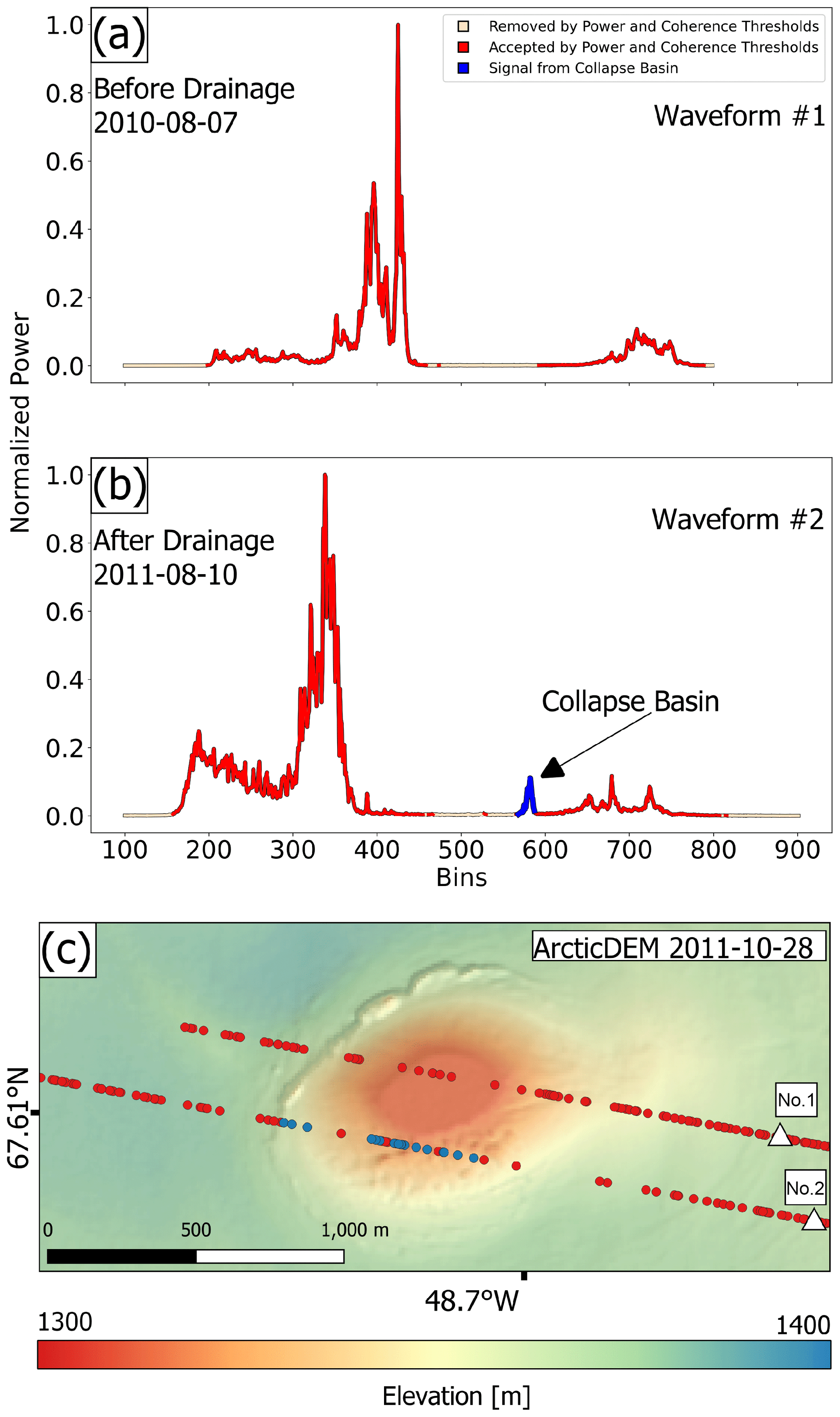
Figure 3(a) CryoSat-2 Level 1b (L1b) data from 7 August 2010 (waveform no. 1) and (b) 10 August 2011 (waveform no. 2) over Lake 1. Dark red sections of the waveform are those accepted by the algorithm thresholds, and the light red sections are not. The blue section in the waveform in (b) is that located over the collapse basin after processing. (c) ArcticDEM scene (28 October 2011) showing where the processed swath points from waveforms no. 1 and no. 2 are located. The satellite nadir position is shown with triangles.
4.1 Filtering of CryoSat-2 data
Figure 4a shows as an example the spatial data coverage of CS2 data over Lake 4, with POCA locations as black circles and swath-processed data in colours according to the elevation. It is clear that the swath-processed data offer an increase in data coverage, which is needed in order to map the small-scale features of the ice surface collapse basins above active subglacial lakes in Greenland since no POCA points are located within the collapse basin (Noël et al., 2015; Andersen et al., 2021). Figure 4b and c show the output of the swath processor when applying a coherence threshold of 0.8 (standard) and 0.5, respectively. In Fig. 4b no swath-processed data points are obtained inside the lake outline, while in Fig. 4c the number of available swath-processed data points increases due to the decreased coherence limit. Decreasing the normalized coherence limit increases the number of generated elevation estimates but increases the noise and errors in the output. Andersen et al. (2021) found that decreasing the coherence limit from 0.8 to 0.6 increased the number of generated data points by 25 % but increased the standard deviation of the crossover elevation difference by 35 %–65 %.
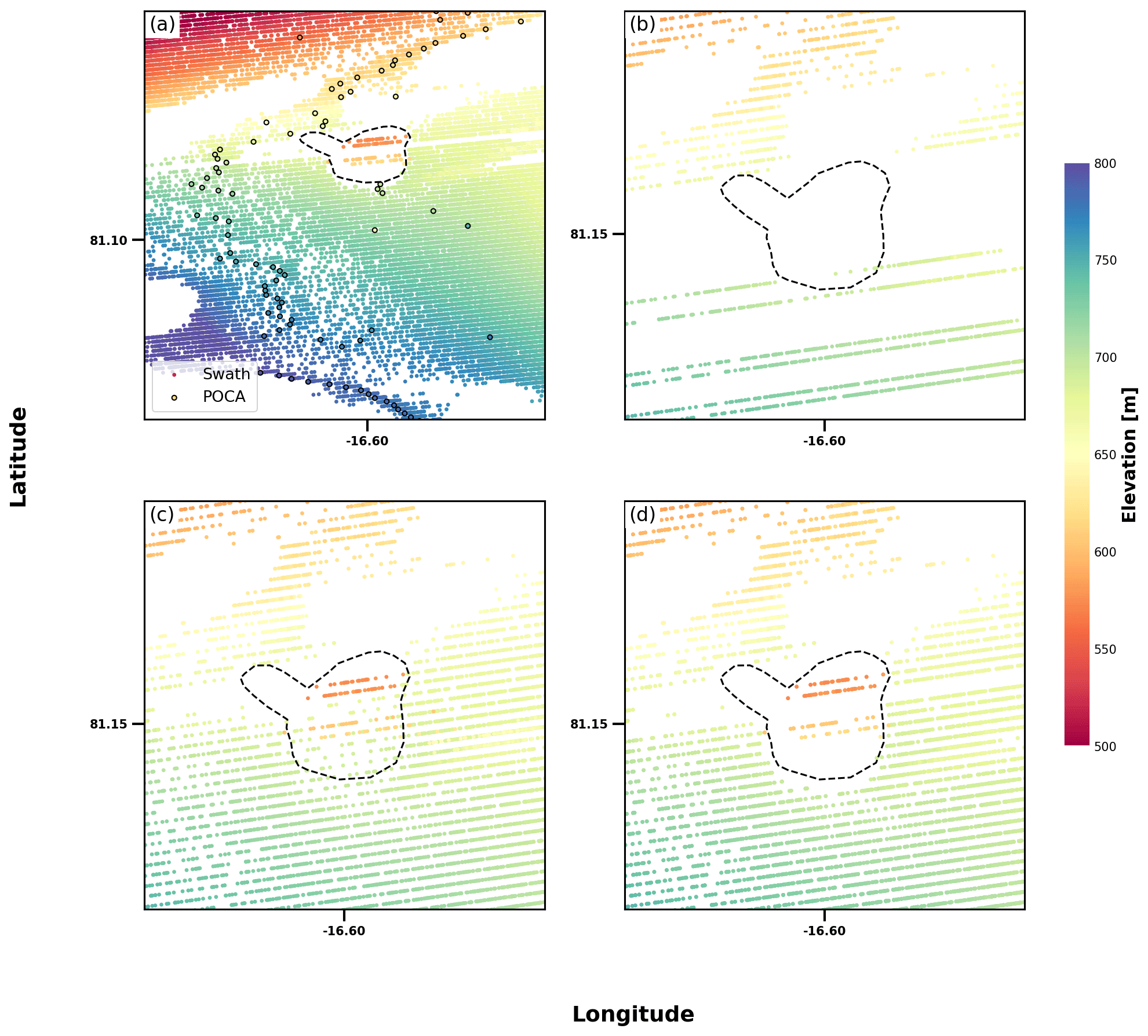
Figure 4(a) POCA and swath-processed elevation data from November 2011 in the area surrounding Lake 4. (b) The standard swath-processed elevation data with a coherence threshold of 0.8. (c) The swath-processed elevation data with a decreased coherence limit of 0.5. (d) The filtered swath-processed elevation data with a decreased coherence limit of 0.5.
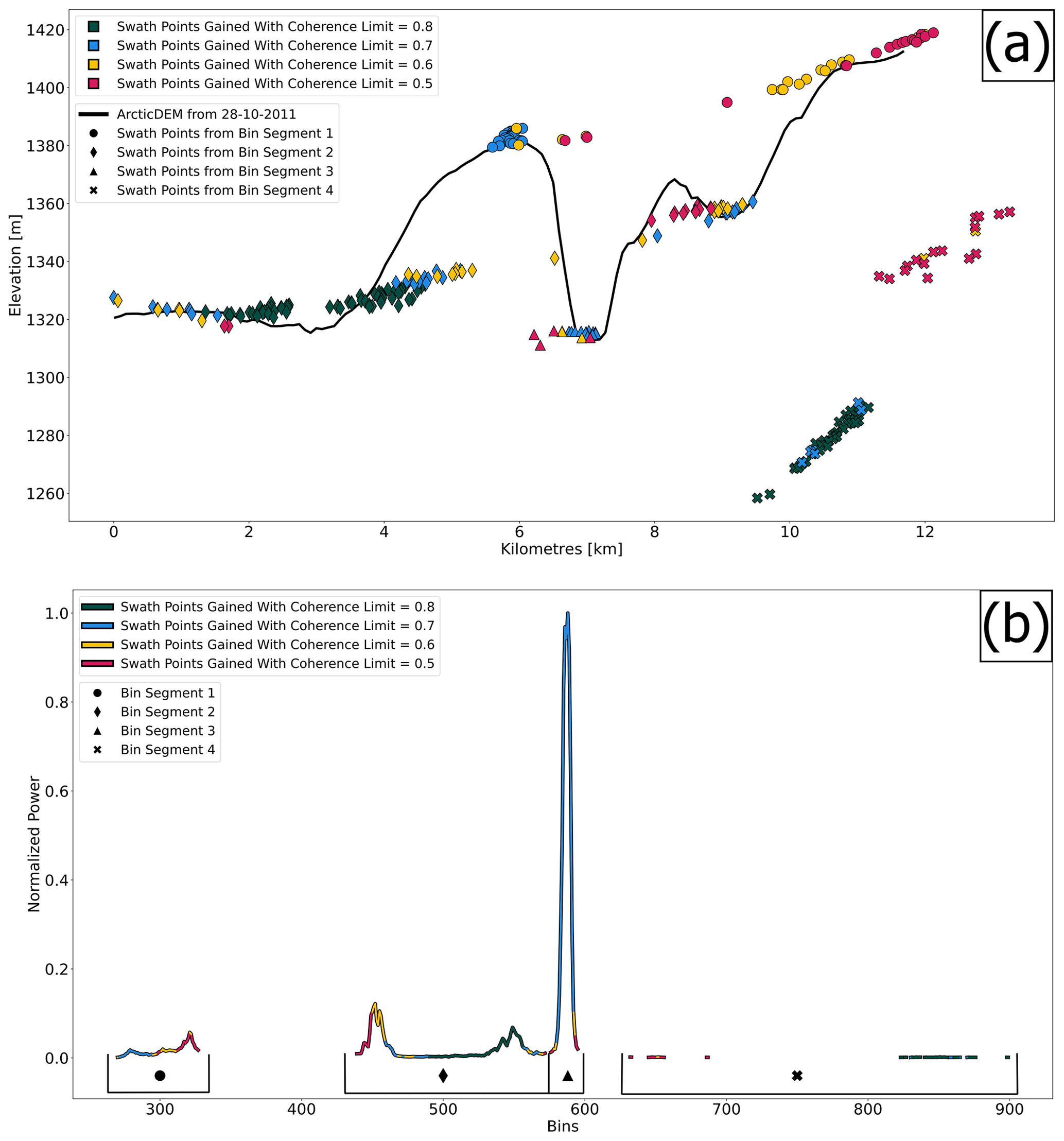
Figure 5(a) Processed swath points from a CryoSat-2 L1b Waveform (7 September 2011) after the drainage event at Lake 1. The colours indicate what coherence limit was used to process each point, and the symbols specify from where on the L1b waveform they are from. The dark green sections of the waveform are those accepted at a coherence threshold of 0.8, and light blue sections are those additionally accepted from lowering the threshold to 0.7. Likewise, the yellow and pink are those for coherence thresholds of 0.6 and 0.5, respectively. The black line is the topography along the swath from an ArcticDEM scene from 28 October 2011. (b) Corresponding CryoSat-2 L1b waveform, with the coloured sections illustrating what waveform part is gained when changing the coherence limit. The waveform is divided into four bin segments labelled by four distinctive symbols. The round points are from the early bin range at ∼300, the diamond shapes are from the range at ∼500, the triangles are from the large peak at ∼600, and the crossed points are from the low-power section after the large peak.
Since lowering the coherence and power thresholds increases the probability of phase unwrapping errors in the L2 elevation product (Gourmelen et al., 2018a), filtering of the generated elevation point data is required to remove erroneous data from the subsequent analysis. Here, filtering based on coherence, power, and range bin numbers of each produced elevation estimate is applied. We find that the swath-processed CS2 data from within the collapse basin and from the surface near the rim have distinct compositions of these three waveform parameters. This clustering in the data allows us to identify and remove erroneous data points by choosing appropriate threshold values for these parameters.
To illustrate these clusters in the data, we show as an example in Fig. 5 some detailed information from a single waveform from 7 September 2011 over Lake 1. The large peak in this waveform might be caused by the reflection from surface water at the bottom of the collapse basin. Figure 5b shows the normalized power in the waveform with colours indicating their corresponding coherence range. The power threshold is fixed at 0.001 at this site. Also, we have divided the waveform bins into four segments and assigned each one a symbol in Fig. 5b.
In Fig. 5a the elevation estimates obtained by the swath processor are shown, together with an elevation profile from an ArcticDEM scene from 28 October 2011, as a black line. The elevation estimated is colour-coded and annotated with a symbol according to Fig. 5b.
From Fig. 5a we can see that when applying a coherence threshold of 0.8, no measurements from the drainage basin (longitude −48.80∘) are obtained. When decreasing the threshold to 0.7, much of the large peak in bin segment 3 is processed, and all the swath points from that bin segment originate from the collapse basin. When setting the threshold to 0.6, we gain a few more points at the basin from bin segment 3, which is beneficial, but we also see that two data points show elevations of ∼1380 m even though they are located above the drainage basin (∼1320 m). These points originate from bin segment 1 and are therefore easy to separate from the other data points from within the drainage basin. Likewise, it is clear from the figure that all measurements from bin segment 4 (crossed points) deviate from the real surface; hence, this cluster of data will be filtered out and will not be used in the analysis.
Even after the removal of data based on this filtering, some erroneous data points might persist over the collapse basin, which are removed in a second step by applying lowest-level filtering to the elevation estimates within the outlined collapse basin so that the cluster of data with the lowest elevation within the defined lake outline is assumed to be representative of the bottom of the collapse basin.
An example of results obtained by swath processing and subsequent filtering over Lake 4 is shown in Fig. 4d, which shows the final elevation estimates after the filtering of the data shown in Fig. 4c. We find that the fraction of removed data depends on the basin's scattering mechanisms and the distance to the CS2 nadir track. Between Fig. 4c and d, there is a reduction of 47 % of data points inside the collapse basin outline.
4.2 Alignment of data sets
We vertically align the three elevation data sets (TanDEM-X, CS2, and ArcticDEM) to account for fluctuations in the surface elevation caused by regional surface mass balance (SMB), for ice dynamics (similar to what was done in Palmer et al., 2015), and for different penetration biases for the radar measurements, typically 0.5–1 m for CS2 and 3–4 m for TanDEM-X (Wessel et al., 2016; Abdullahi et al., 2019). The vertical alignment is done by defining anchor points close to the rim of each subglacial lake surface depression in the earliest available DEM. All consecutive DEMs are height corrected to align with the reference DEM at the location of the chosen anchor point. To vertically align the discrete CryoSat-2 swath data to the DEMs, the median of the difference between CS2 points close to the collapse basin and the reference DEM was used to correct for the vertical bias. This procedure ignores different penetration depths at the surface on the rim, but it preserves the relative heights from the top of the rim to the bottom of the depression for each sensor. This alignment allows us to focus on the local height change within the collapse basin likely caused by the dynamic hydrological processes. The maximum vertical offset was 12 m, but for the vast majority of the data sets the alignment correction was less than 3 m.
The data are also aligned horizontally to account for ice flow. Lakes 1–3 are located in the upper ablation zone in the southwestern part of the GrIS, where the ice flows in a westerly direction. Optical imagery and the three data sets provide evidence that the collapse basins advect with the ice flow. Figure 6 shows the drift of the collapse basin over Lake 1 in the period 2011–2021. ArcticDEMs were used to create the collapse basin outlines between 2011 and 2017, while Landsat-8 was used until 2021. We compared an ArcticDEM scene and a Landsat-8 image from the summer period of 2015 and found no considerable visual bias in the basin outline. The basin drifts in a westerly direction and decreases 95 % in surface area from 2011–2021 as the subglacial lake gradually recharges and/or the collapse basin is filled due to ice flow and deformation. This movement results in a horizontal offset of 100 m between the surface depression in 2021 and its initial location in 2011.
To consistently track the evolution of the depth of the collapse basins, even when they change location due to ice flow, we horizontally align the data sets by correcting for the observed local ice flow using MEaSUREs Greenland Ice Sheet Velocity Map from InSAR data (Joughin et al., 2010, 2015) and greenland ice velocity from Sentinel-1 data, edition 2 (Solgaard et al., 2021; Solgaard and Kusk, 2021). At the location of Lake 4, the ice flow velocity is found to be <17 m yr−1, and we see no evidence in the elevation that this collapse basin has moved over time. One reason for this can be that the subglacial lake drains again in the observational period, which could make the potential ice flow less evident since the collapse basin is re-formed over the stationary location of the subglacial lake. Therefore, no horizontal alignment was applied at Lake 4.
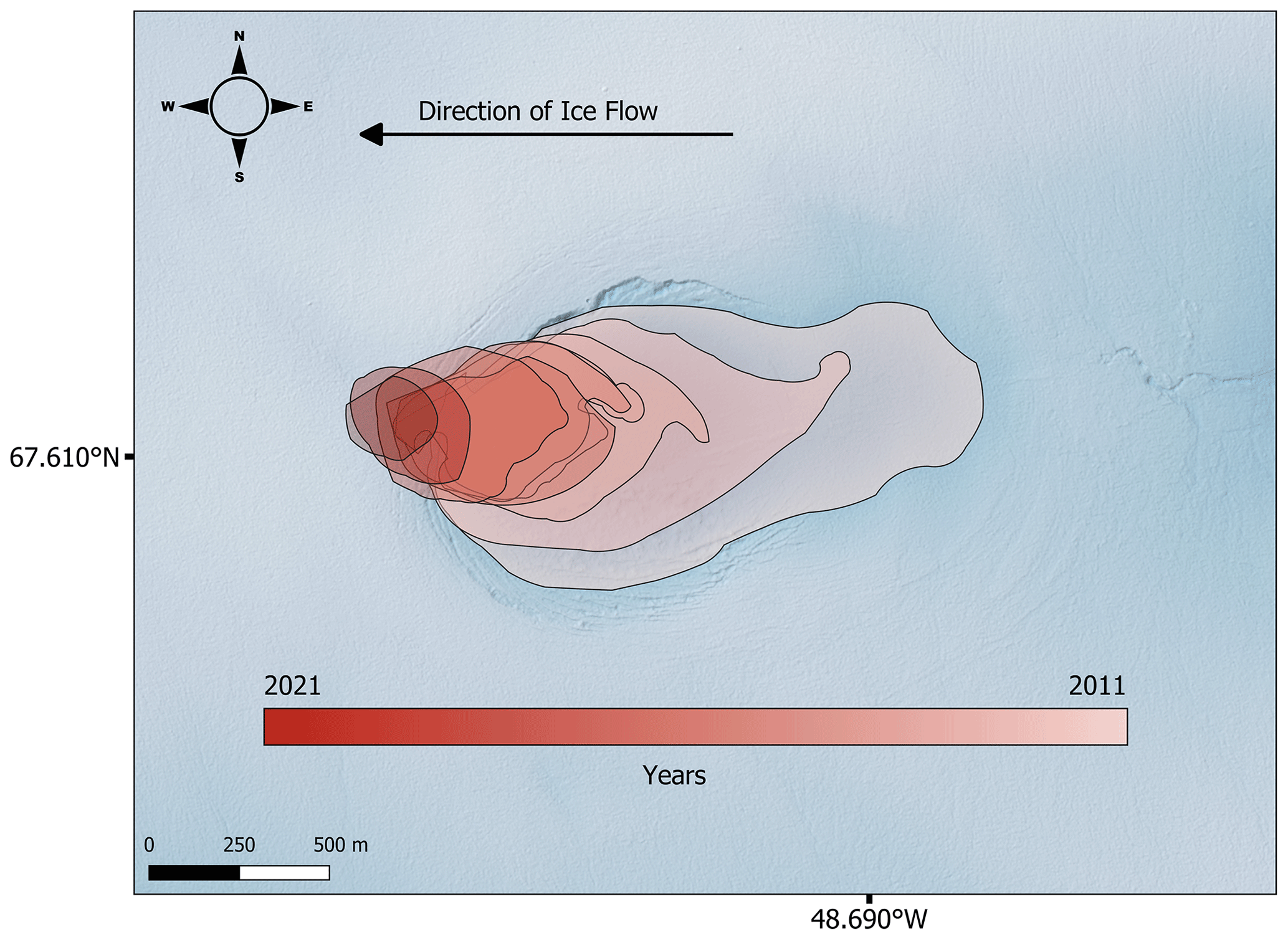
Figure 6The horizontal drift of the collapse basin over Lake 1 during the period from 2011 to 2021. ArcticDEMs were used to create the collapse basin outline between 2011 and 2017, while Landsat-8 images were used until 2021. The basin drifts in a westerly direction, and the surface area decreases substantially.
4.3 Time series of deepest point
The temporal evolution of the depth and shape of the collapse basins is controlled by local factors including refilling of the subglacial lake, SMB, and ice dynamics. Here, we determine the location of the deepest point within a basin. Lake 4 is the largest lake with a relatively flat 1000 m bottom diameter in contrast to the 100 to 400 m ground diameter of Lakes 1–3. We define the deepest point based on the first DEM in which the basin is detected and use the temporal change in elevation of this location as a measure for the evolution of the subglacial lake. For each time-stamped ArcticDEM and TanDEM-X strip, all grid points within a distance of 50 m from the initially deepest point were sampled as this ensures enough data to calculate a robust mean and standard deviation (σ) while still avoiding sampling of the slanting basin walls. Due to the scattered coverage and the limited number of CS2 data points, the corresponding estimate of the basin depth at Lake 1 is derived from all CS2 point data within the outline of the basin. We only used CS2 track crossings for which 10 or more points were available within the basin and points were within 5σ of all data within the basin. The horizontal alignment and the filtering of the CS2 swath data ensure that we do not need to change the manually delineated basin outline through time. At the substantially larger Lake 4, we sampled all CS2 points within 400 m from the deepest point, thus not sampling the inclining basin floor. We compute the mean of each of the sampled data sets and use this as the value for the elevation of the deepest point. Their standard deviation represents the spatial variability in these data, and we use 2σ as the error bar on the depth estimate but note that this is not a measure of their true accuracy.
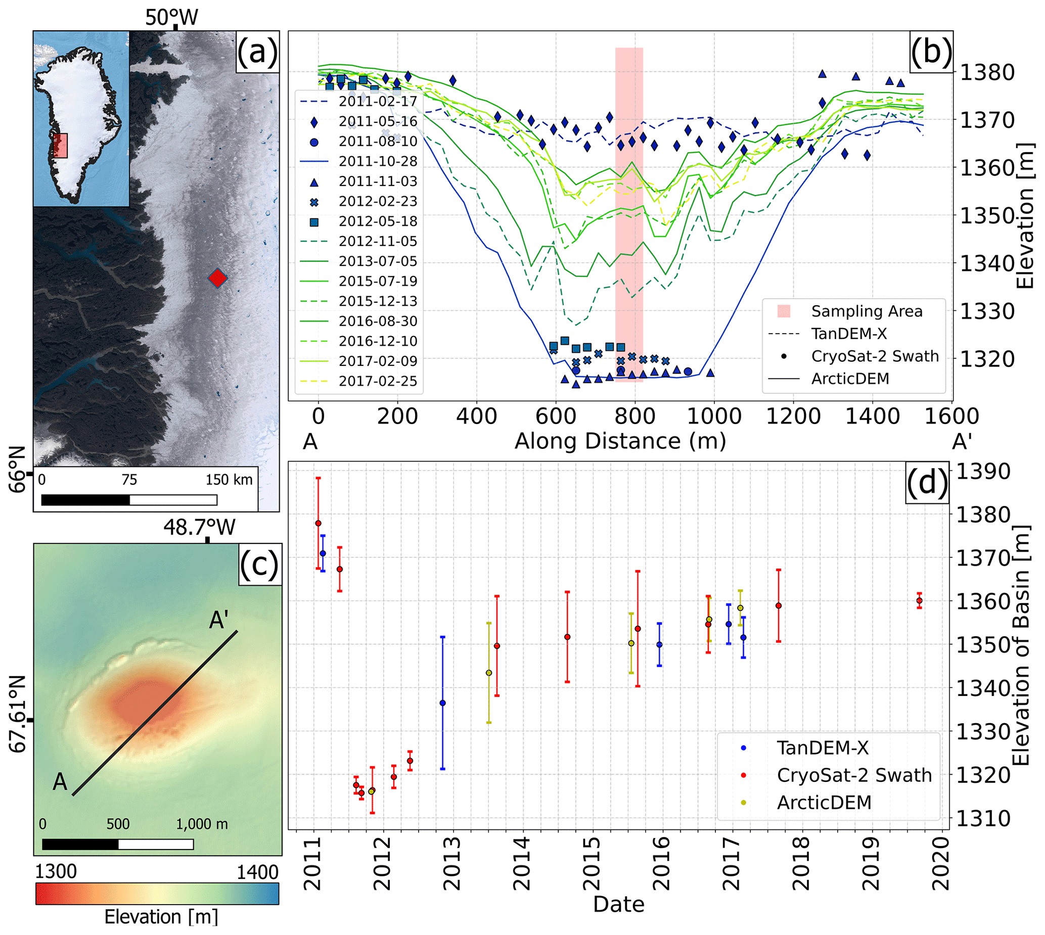
Figure 7Lake 1: (a) the location of the collapse basin on a background image from Landsat-8 from 2019. (b) Elevation profiles from the three aligned data sets; TanDEM-X is the dashed line, CryoSat-2 data are represented by symbols, and ArcticDEM is the solid line. (c) The collapse basin as seen in an ArcticDEM on 28 October 2011. Line A–A' is the profile used in (b). (d) Time series of the deepest point of the lake basin from TanDEM-X (blue), CS2 (red), and ArcticDEM (yellow). The depth is based on sampling within the area indicated by red in (b).
For each lake site, we present the temporal evolution of the ice surface collapse basins both by height profiles across the basins and as a time series of the elevation of the deepest point in each basin.
Our findings for Lake 1 are presented in Fig. 7. Figure 7b shows the ice sheet elevations of Lake 1 along the A–A' profile shown in Fig. 7c. The location of A–A' is adjusted through time to account for ice flow. With CS2 swath processing, it was possible to extract point measurements from 12 satellite tracks passing over Lake 1. The CS2 data are point observations of elevations and do not provide full surface coverage like the TanDEM-X and ArcticDEMs do. Hence, the CS2 observations plotted are those data points that are located closer than 180 m to the A–A' profile. This distance ensures that data from all satellite crossings are represented. The colours of the height profiles indicate the time of the measurements, with darker colours for the start of the measurement period (2011) and lighter colours for the end of the measurement period (2017). We find that a TanDEM-X DEM from 17 February 2011 and CS2 data from 18 May 2011 show that the surface is generally flat, indicating that the ice surface collapse basin has not yet been created. The first measurements that show signs of a collapse basin are a CS2 crossing from 10 August 2011, which detects a surface depression with a depth of approximately 60 m with a flat surface at the bottom. Over time, the collapse basin decreases in size (both in depth and area), but a depression is still evident in the most recent data set, which is an ArcticDEM from 2 September 2017. For clarity, we have not shown all available data sets in Fig. 7b. Figure 7d shows the temporal evolution of the depth of the deepest part of the collapse basin (Sect. 4.3), and it shows that the basin depth did remain stable during the winter of 2011/2012 following the collapse. In the period from February 2012 to July 2013 TanDEM-X and ArcticDEM DEMs reveal a rapid rise in the depression floor over the 15-month period from February 2012 to July 2013, during which the depth is reduced to about 25 m. The results show a slower decrease rate after 2015. At the time of the last measurement by CS2 in late 2019, the depth is approximately 15 m, which agrees within the error bars with the height from an ArcticDEM from September 2017. The collapse basin filling rate can be divided into a fast basin uplift of ∼13 m yr−1 in the period 2011–2015 and a period with no substantial uplift from 2015–2019.
Figures 8 and 9 show the data available for Lake 2 and Lake 3, respectively. While several TanDEM-X DEMs covering these sites were successfully produced, we were not successful in obtaining any useful CS2 swath-processed data over these subglacial lakes. The collapse basins over Lakes 2 and 3 span smaller areas than those over Lakes 1 and 4, and they are also shallower, which could be the reason for the lack of CS2 data here. The early 2011 TanDEM-X observations of Lake 2 show no signs of a collapse basin being formed; however, the four subsequent DEMs (July 2012 to April 2013) clearly show the imprint of a collapse basin (see Fig. 8b). The collapse basin had a depth of approximately 15 m, which did not change from July 2012 to April 2013, while in the period from April 2013 to December 2013 it appears to fill up completely. After the 2013 melt season, one DEM (TanDEM-X on 26 December 2016) shows a collapse basin feature with a depth of 10 m, while all others (indicated with the light red area in Fig. 8d) show a relatively flat surface at pre-collapse elevations. These observed flat surfaces are the result of the collapse basin filling with surface water, as confirmed by optical images close in time to the DEMs. At Lake 3, the earliest TanDEM-X observations from 20 January 2011 show a surface depression with a maximum depth of approximately 20 m (Fig. 9b). Similar to Lake 2 most DEMs available at Lake 3 show no surface depression after the 2013 melt season (Fig. 9b and d), and only two near-coincident ArcticDEMs from the summer of 2015 show a small surface depression of approximately 10 m.
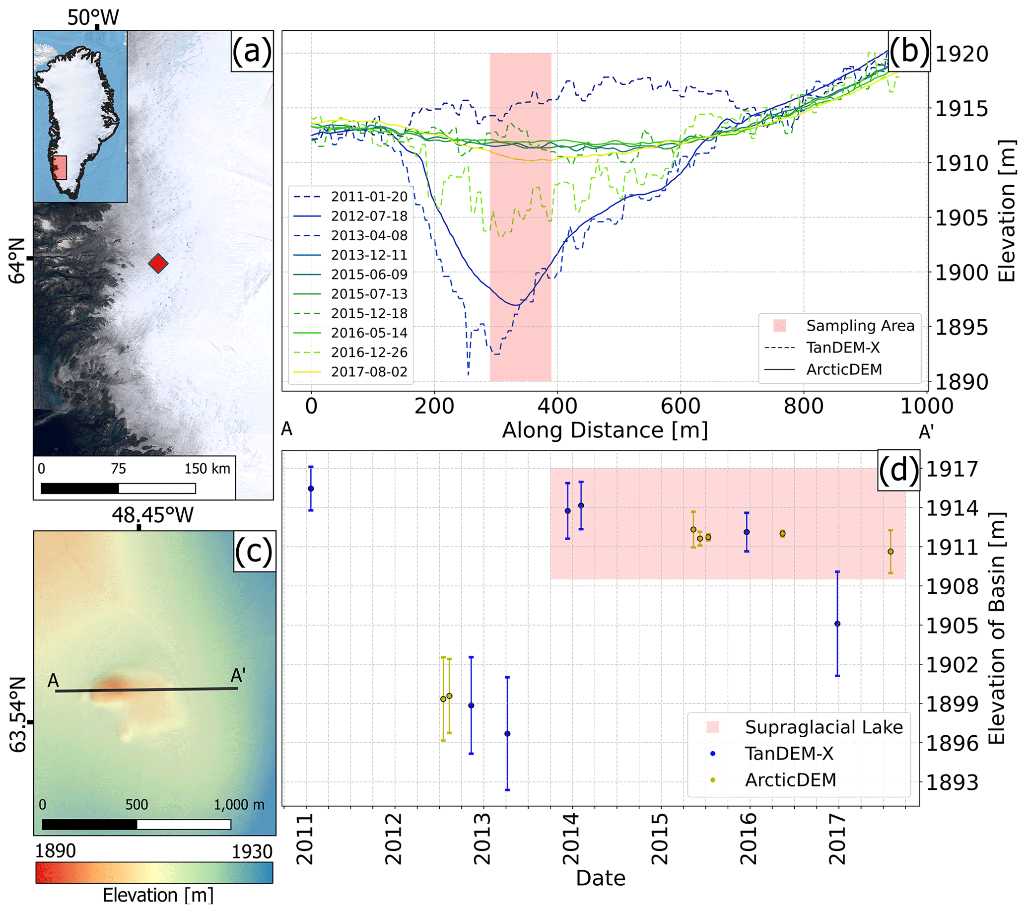
Figure 8Lake 2: (a) the location of the collapse basin on a background image from Landsat-8 from 2019. (b) Elevation profiles from the two aligned data sets; TanDEM-X is the dashed line, and ArcticDEM is the solid line. (c) The collapse basin as seen in an ArcticDEM on 18 July 2012. Line A–A' is the profile shown in (b). (d) Time series of the deepest point of the collapse basin from TanDEM-X (blue) and ArcticDEM (yellow). The light red box marks those estimates where surface water was present.
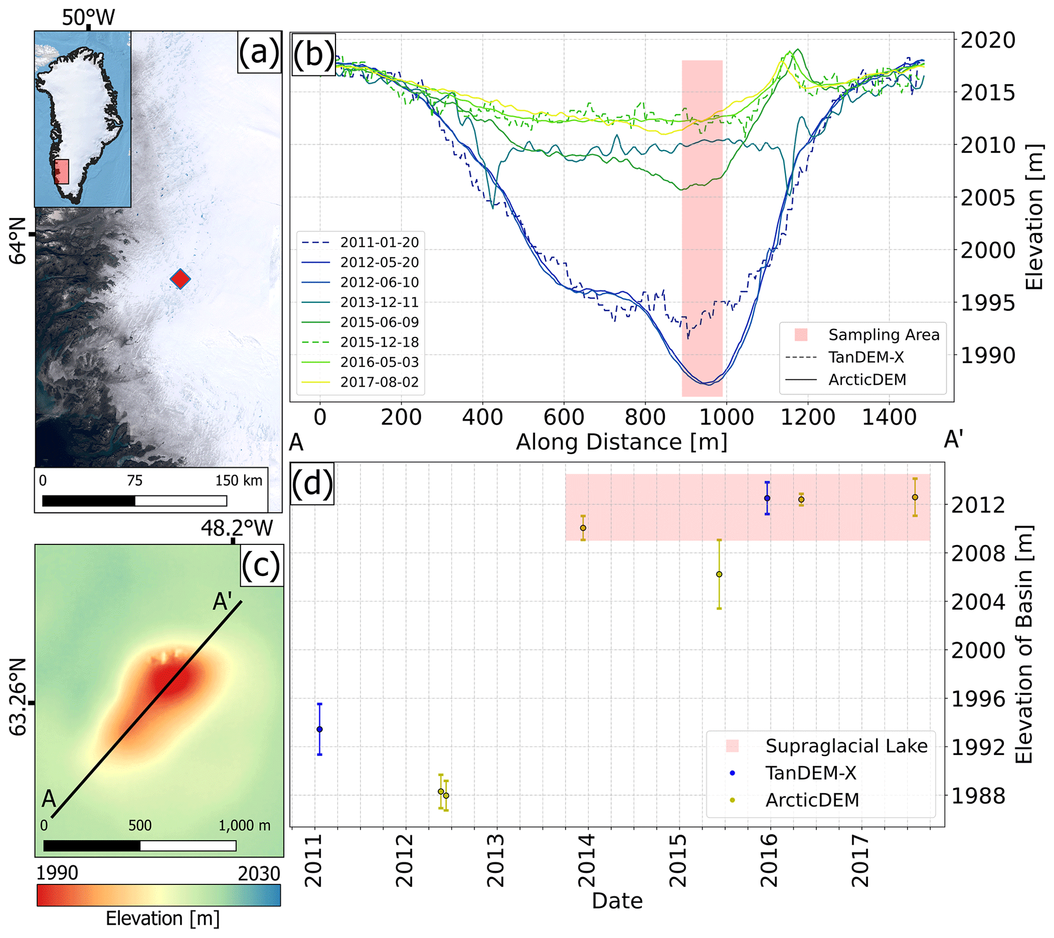
Figure 9Lake 3: (a) the location of the collapse basin on a background image from Landsat-8 from 2019. (b) Elevation profiles from the two aligned data sets; TanDEM-X is the dashed line, and ArcticDEM is the solid line. (c) The collapse basin as seen in an ArcticDEM on 20 May 2012. Line A–A' is the profile shown in (b). (d) Time series of the deepest point of the collapse basin from TanDEM-X (blue) and ArcticDEM (yellow). The light red box marks those estimates where surface water was present.
Figure 10 shows our results over Lake 4 on the Flade Isblink Ice Cap in northeastern Greenland. For this collapse basin, the largest of those analysed, several CS2 crossings provide elevation measurements of the collapse basin, and also several TanDEM-X DEMs are available. A TanDEM-X DEM from January and CS2 data from February 2011 show a flat ice surface in the region of interest. The first data set to observe the collapse basin is CS2 swath data from late November 2011, showing a relatively flat bottom of a collapse basin with a depth of approximately 95 m. The following data set is also from CS2 data (February 2012), and it reveals an upward movement of the collapse basin floor of more than 5 m since the previous measurements 3 months earlier. As the collapse basin is filled over time, we observe the development of a dome shape at the base of the collapse basin. By April 2017, the last available DEM data (TanDEM-X) show that the height of the top of the dome was 20 m from reaching the pre-collapse surface elevation. The filling rate of the collapse basin changes over time, with a faster rate of elevation change (∼38 m yr−1) immediately after the collapse (November 2011–March 2013) than in the following years, when the rate of elevation change in the deepest point decreased to ∼11 m yr−1 (for the period after March 2013). To maintain a visually clear plot, not all data sets are shown in Fig. 10b. Figure 10d shows the temporal evolution of the deepest point of the collapse basin until 2021. CS2 swath-processed data after 2017 indicate that Lake 4 drains again in the summer period of 2019, creating a negative elevation change of ∼12 m. The lake seems to quickly recharge from this drainage during the melt season of 2020.
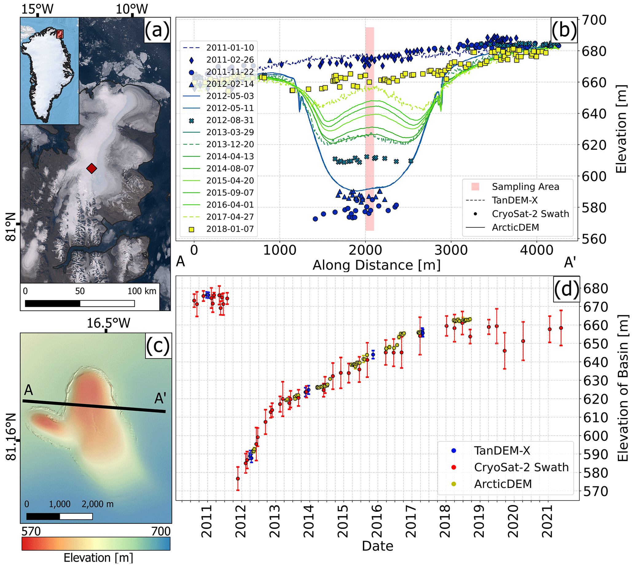
Figure 10Lake 4: (a) the location of the collapse basin on a background image from Landsat-8 from 2019. (b) Elevation profiles from the three aligned data sets; TanDEM-X is the dashed line, and CryoSat-2 is represented by symbols and ArcticDEM is the solid line. (c) The collapse basin as seen in an ArcticDEM on 3 May 2012. Line A–A' is the profile used in (b). (d) Time series of the deepest point of the collapse basin from TanDEM-X (blue), CS2 (red), and ArcticDEM (yellow). The depth is based on sampling within the area indicated by red in (b).
6.1 Lake 1
Over Lake 1 the swath-processed CS2 data and the TanDEM-X data provide new insight into the temporal evolution of the collapse basin. The CS2 data agree within the error margins with near-coincident ArcticDEM and TanDEM-X elevations, giving us confidence in their validity. The availability of the CS2 and TanDEM-X data greatly increases the temporal resolution of data. Compared to previous studies (Palmer et al., 2015; Howat et al., 2015) based on optical imagery with less than one observation per year, we are now able to extract multiple observations for each year, and our results confirm the timing of the drainage event of the subglacial lake. Notably, the addition of CS2 observations during 2011 and 2012 allows us to conclude that no substantial recharge of the subglacial lake occurred between August 2011 and May 2012 (see Fig. 7b), while recharge is observed between May and November 2012. The fact that the rate of recharge was insignificant during a period outside the melt season supports the hypothesis proposed by Palmer et al. (2015) and Howat et al. (2015) that the subglacial lake is primarily driven by surface meltwater drained to the bed through moulins during the melt season. We further hypothesize that the infilling of the collapse basin after 2014/2015 is likely primarily caused by snowfall and ice flow and less by the recharging of the subglacial lake due to the fact that the centre of the collapse basin moves away from the location of the subglacial lake due to ice flow. The uplift rate due to filling usually slows over time due to the geometry of the lake. This kind of glacier response was further modelled and investigated by Aðalgeirsdóttir et al. (2000), where the Vatnajökull Ice Cap in Iceland showed a similar modelled response after a subglacial drainage event created a surface depression.
6.2 Lakes 2 and 3
It was not possible to successfully obtain any CS2 swath-processed data over Lake 2 and Lake 3. This is likely due to their small size (collapse basin areas less than 0.6 km2), which does not allow for adequate waveform signals with a coherent phase difference. However, with the availability of several TanDEM-X DEMs covering both lakes, we are able to augment existing observations from Bowling et al. (2019) and gain further insights into their temporal characteristics. Previous studies that relied exclusively on ArcticDEMs could not conclude on the timing of the drainage event over Lake 2 (Bowling et al., 2019), but the addition of TanDEM-X scenes reveals that the drainage event did not occur earlier than January 2011. Optical imagery indicates that surface water is present in the collapse basins several times after the subglacial lakes drain. At Lake 2 Landsat-8 imagery from spring–summer 2015 shows first a flat surface followed by water presence, indicating a frozen supraglacial lake that melts, which then drains in the summer period of 2016. This is clear in Fig. 8b, where a flat surface is present in the elevation profiles in 2015, which then shows a collapse basin in the TanDEM-X profile from late 2016.
At Lake 3 Landsat-8 images from autumn 2013 and spring 2014 show a flat surface, also suggesting a frozen supraglacial lake which then melts and drains during summer 2014. This is also clear in the elevation profiles in Fig. 8 where the acquisition from late 2013 shows a flat surface, but then in spring 2015 the collapse basin is visible again. Based on this finding, we suggest that the elevation profiles from the DEMs highlighted with a light red box in both Figs. 8d and 9d map the height of a supraglacial lake forming in the surface depressions rather than the actual surface depressions. Disregarding those estimates that we believe are associated with surface water, we conclude that the collapse basins over Lake 2 and Lake 3 have not completely filled up by the latest available measurements (late 2016 for Lake 2 and mid-2015 for Lake 3).
6.3 Lake 4
Willis et al. (2015) reported that the collapse basin over Lake 4 had a depth of approximately 70 m on 3 May 2012, and TanDEM-X DEMs processed for this study confirm this estimate (Fig. 10b). With the inclusion of CS2 data from November 2011, we can furthermore conclude that the collapse basin had been at least 95 m deep prior to May 2012, suggesting that the collapse basin likely was more than 100 m deep at the time of the collapse. We arrive at this depth by using the observed average rate of infilling during the period November 2011 to March 2013 (∼30 m yr−1) and then assuming that this infilling rate is representative of the period from the collapse in August/September 2011 (Willis et al., 2015) to our first post-collapse measurement in November 2011.
Willis et al. (2015) also showed an uplift rate of ∼9 m yr−1 based on three near-coincident ArcticDEM scenes in May 2012. With the inclusion of CS2 in the analysis, we find that the uplift rate appears to be larger, as we find a relatively constant uplift rate of ∼32 m yr−1 in the period of November 2011 to the end of 2012. This indicates that a substantial level of lake infilling happened within a year of the drainage event, indicating that meltwater is readily available at this site. The lake appears to fill during winter months, indicating that at least some of the input is basal meltwater, although the study by Liang et al. (2022) argues that the long-term recharge of the lake is dominated by a seasonal influx of surface meltwater. The high-resolution data sets gathered here also give insights into the physical processes driving the refilling of a subglacial lake collapse basin. At Flade Isblink Ice Cap (Lake 4), we observe a dome forming in the central part of the collapse basin as it refills. The CS2 data also observed a ∼15 m drop in elevation (Fig. 10d) between 31 May and 24 August 2019, indicating that Lake 4 partially drained a second time but that the event is substantially smaller than that in 2011. The surface lowering in 2019 is also documented from ICESat-2 data by Liang et al. (2022), who identified it as a drainage event. They also found that this event caused the ice velocity downstream from the lake to abruptly but briefly increase. Further investigations into available meltwater sources and local ice cap settings are necessary in order to understand why Lake 4 did not drain completely in 2019.
6.4 Data limitations
We are able to retrieve CS2 swath-processed elevation data over Lake 1 and Lake 4 prior to drainage, immediately after the drainage, and during the following recharge period. In Figs. 7d and 10d the CS2 swath data provide better temporal coverage than TanDEM-X and ArcticDEM just after the collapse. When applying the CS2 swath processing, careful filtering based on coherence, power, and bin number is applied. We suggest that when the surface depressions are filled over time, the signal from the bottom does not stand out as clearly in the waveform because it is located closer to the surface returns in the waveform. This could indicate that CS2 swath processing is useful to detect primarily the bottom of only the relatively deep surface depressions with a sizable area and may explain why it was not possible to obtain data over Lakes 2 and 3, which are not as deep or large as Lakes 1 and 4. The fact that the bottom of the collapse basins are flat at Lake 1 and Lake 4 further aids the elevation retrievals immediately after the collapse because the flat bottom makes the surface a better reflector for the radar. Due to the need for careful filtering and tuning of the CS2 swath processor, the CS2 data are not ideal for finding and locating subglacial lake activity since the analysis is dependent on available DEMs. We find that another limiting factor for the success of CS2 swath processing for subglacial lake mapping is that the satellite track must pass directly over the surface depression for bottom echoes to be retrieved. If the surface feature is located too far off-nadir, we do not obtain any valuable data. This limits the use of CS2 to very specific cases of subglacial lake activity; however, as seen above, we do find useful satellite crossings for well-developed collapse basins.
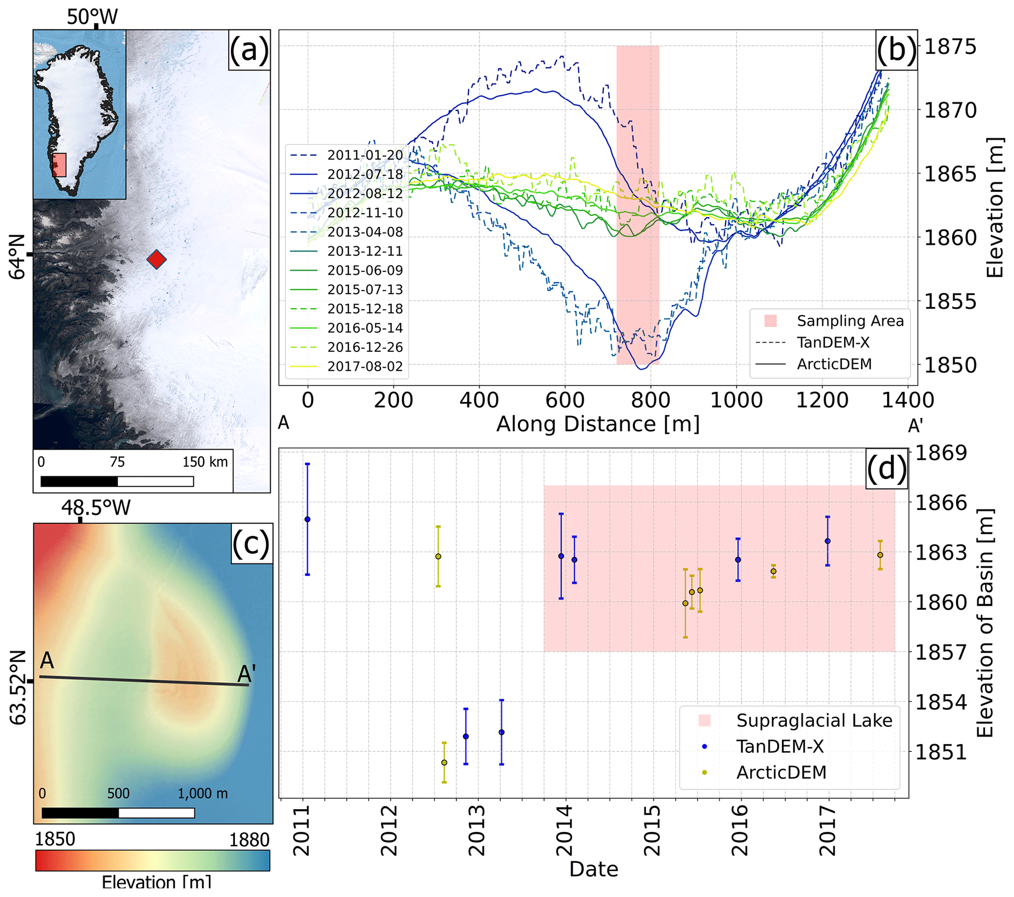
Figure 11Possible active subglacial lake: (a) the location of the collapse basin on a background image from Landsat-8 from 2019. (b) Elevation profiles from the two aligned data sets; TanDEM-X is the dashed line, and ArcticDEM is the solid line. (c) Possible collapse basin as seen in an ArcticDEM on 12 August 2012. Line A–A' is the profile used in (b). (d) Time series of the deepest point of the lake basin from TanDEM-X (blue) and ArcticDEM (yellow).
To minimize the elevation changes caused by different surface penetration and the elevation changes caused by surface mass balance, we vertically align all the data sets at the rim of the collapse basins (Sect. 4.2). This implies an assumption that the surface mass balance and the ice properties within the collapse basin are the same as at the rim. This is likely associated with an error since, for example, snow conditions in the depression may differ from those around it. Additionally, the surface penetration depth of both CS2 and TanDEM-X can vary spatially and could potentially be different in the collapse basin from the surrounding areas. At present, we do not include this error in our estimates since we do not have the means to quantify it.
6.5 New subglacial lake
In our analysis of Lakes 2 and 3, we identified an interesting signal on the ice sheet, which to our knowledge has not been described previously. The signal is located southwest of Lake 2 and appears to show indications of a new, active subglacial lake (here denoted as Lake 5). The location and the elevation profiles from ArcticDEMs and TanDEM-X DEMs from Lake 5 are shown in Fig. 11. The elevation data show a dome-shaped feature on the surface in January 2011 and July 2012 (Fig. 11b). Between 18 July 2012 and 12 August 2012, a rapid ∼15 m surface elevation lowering occurs and a feature resembling a collapse basin is formed. The low point of the surface depression is shifted horizontally compared to the dome. To more precisely determine the timing of the formation of the collapse basin, we also investigated optical imagery from the area and found that in a Landsat-7 image from 25 July 2012, there are no indications of a collapse basin (See Appendix, Fig. A1), suggesting a lake drainage between 25 July and 12 August 2012. This drainage event coincides with the unprecedented melt event in July 2012 across the GrIS (Nghiem et al., 2012). As this newly discovered Lake 5 is located approximately 2 km downstream of Lake 2 (see Appendix A, Fig. A2), we hypothesize that the two could be hydrologically connected. For Lake 2 we know from a TanDEM-X DEM that the collapse did not occur in January 2011 (Fig. 8b), and Landsat-7 imagery further does not show a collapse basin either in early June 2012 (Fig. A3). Although the image is not very clear, possibly due to snow cover, we see a body of surface water that partially intersects with the outline of the collapse basin as observed in an August ArcticDEM from 2012, indicating that a local depression had not yet formed in June 2012. The following ArcticDEM and Landsat-7 images from 18 July 2012 show a distinct collapse basin after the draining event (Figs. 8 and A3). Therefore, we can constrain Lake 2 to have likely drained between 9 June and 18 July 2012, which is prior to but temporally close to the draining of subglacial Lake 5 between 25 July–12 August 2012. A possibility is that the two lakes are hydrologically connected, which would to our knowledge be the first indication of hydrologically connected subglacial lakes in Greenland, indicating that water is transferred from one lake to another following a draining event. It is also possible that the coincident drainage of the two lakes was independently triggered by the large amount of surface meltwater available in the summer of 2012. The small size of the investigated subglacial lakes makes it difficult to assess routing pathways at the bedrock considering the limited spatial resolution of available data sets like BedMachine v4. Hydrologically connected lakes have already been documented in Antarctica (Wingham et al., 2006; Smith et al., 2017), and their influence on the subglacial system has been investigated (Malczyk et al., 2020). It should be noted that neither Lake 2, Lake 3, nor Lake 5 is detected in the new study by Fan et al. (2023) likely because they are not active in the period covered by ICESat-2, which hampers further investigations into the inter-connectivity of Lakes 2 and 5.
The importance of subglacial lakes to the hydrology of the Greenland Ice Sheet and surrounding glaciers and ice caps is not well understood largely due to a lack of observations. In this study, we have investigated elevation changes over four Greenlandic subglacial lakes, which previous studies have identified by the presence of a collapse basin at the ice surface. We demonstrate how the inclusion of CS2 swath-processed data and TanDEM-X DEMs in addition to ArcticDEMs improves the mapping of subglacial lake activity in Greenland, demonstrating that these and similar data sets should be included in future analyses in order to increase the temporal resolution of the observational records. The small size of the subglacial lakes in Greenland provides a challenge for satellite radar altimetry, and we are only able to recover useful CS2 data over the two largest collapse basins. The TanDEM-X mission provides a valuable additional elevation data source for all lakes throughout the entire investigated time span (2011–2018). Both TanDEM-X and CS2 data agree well with the ArcticDEM data when we vertically align them at the rim of the collapse basins.
The use of TanDEM-X DEMs and CS2 data substantially increase the sampling frequency over the four subglacial lake sites. For example, the number of measurement epochs increased from 5 from ArcticDEM alone to 22 when including Tandem-X and CS2 over Lake 1 for the time period 2011–2018. Over Lake 1, the addition of CS2 data during the winter of 2011/2012 showed that no substantial recharge of the subglacial lake occurred during this period. Previous literature did not conclude on the timing of the drainage event over Lake 2, but the inclusion of TanDEM-X scenes shows that the drainage happened in the period between 20 January 2011 and 18 July 2012. CS2 data show that the initial depth of the collapse basin over Lake 4 is ∼35 % deeper (approximately 95 m in late November 2011) than previously found based on ArcticDEMs and that the filling rate of the collapse basin changes over time. Finally, we identified a signal that could stem from a previously undetected active subglacial lake in the vicinity of Lake 2. The improved temporal resolution also indicates that this new lake could possibly be hydrologically connected to its upstream neighbour Lake 2, but further studies are required to confirm if this is the case.
In the area of Lake 2, we used Landsat-7 imagery to establish if the timing of the draining is connected to the lake which is observed approximately 2 km downstream.
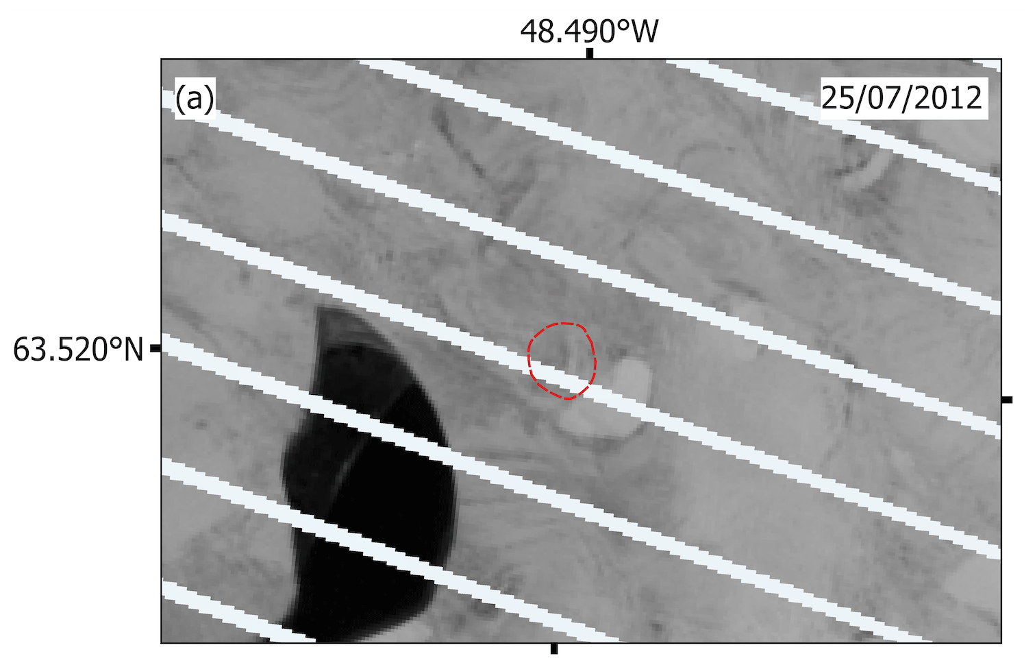
Figure A1Landsat-7 images taken on 25 July 2012 over Lake 5 showing no signs of a collapse basin. The red outline indicates the collapse basin outline as created from an ArcticDEM from 12 August 2012.
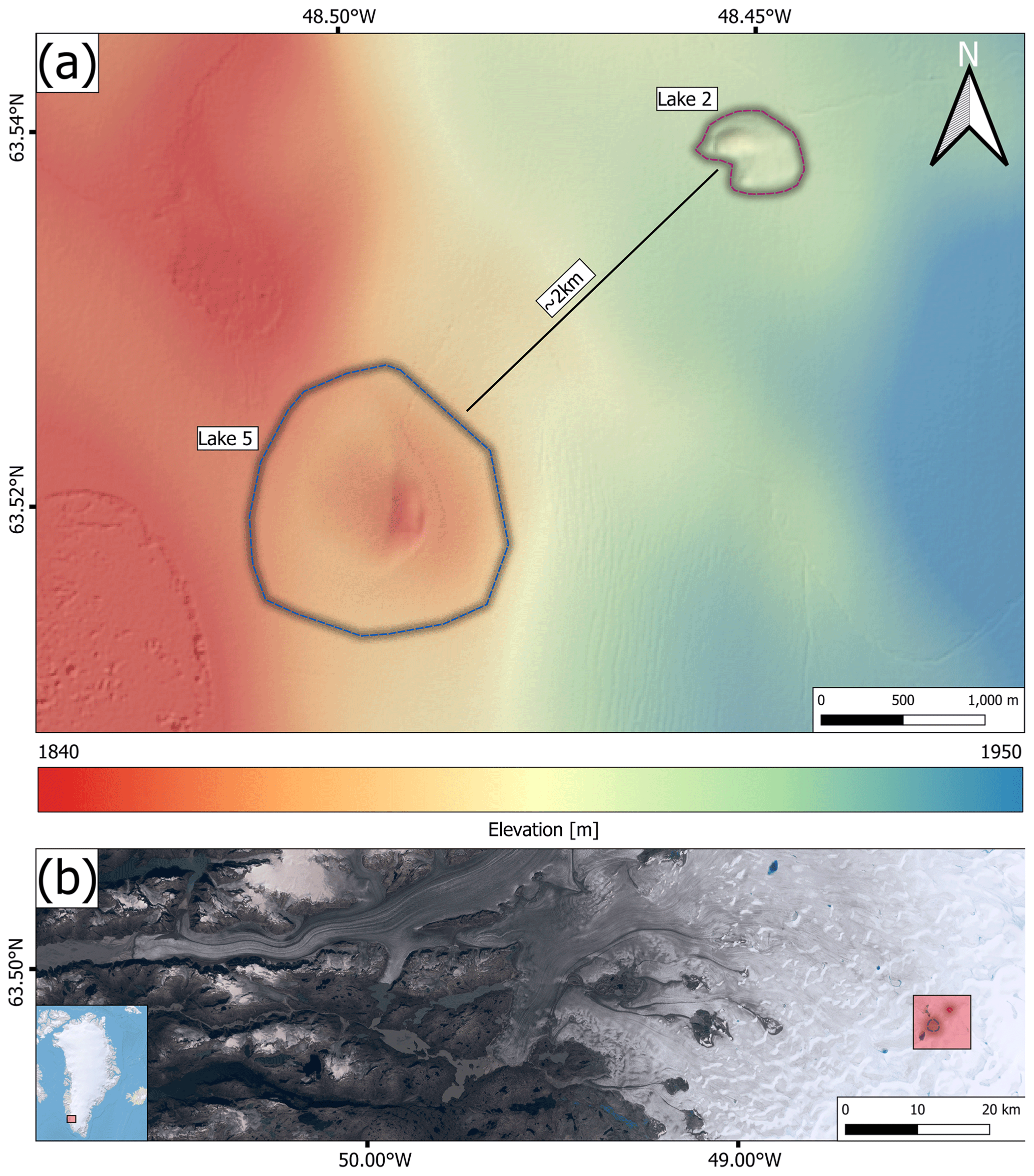
Figure A2(a) Location of Lake 2 relative to Lake 5 shown in an ArcticDEM. (b) Overview of the two lakes' locations on a background image from Landsat-8 from 2019.
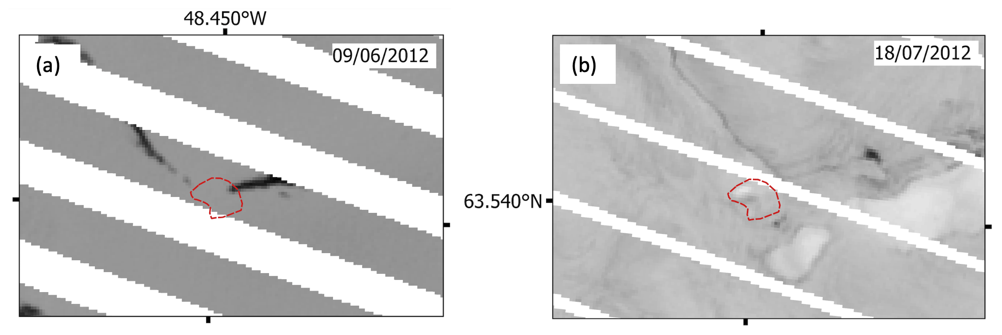
Figure A3(a) Landsat-7 images taken on 9 June 2011 and (b) from 18 July 2012 of the surface before and after the Lake 2 collapse basin had formed. The red outline shows the collapse basin outline as created from an ArcticDEM observed on 18 July 2012.
CryoSat-2 SARIn data are provided by the European Space Agency (ESA) and are freely available on ESA's home page: https://science-pds.cryosat.esa.int/#Cry0Sat2_data/Ice_Baseline_D/SIR_SIN_L1 (ESA, 2023). The TanDEM-X data were provided by the German Aerospace Center (DLR) via TanDEM-X CoSSC proposal XTI_GLAC7335. We used ice velocity data from https://doi.org/10.5067/OC7B04ZM9G6Q (Joughin et al., 2015) and ice velocity maps produced as part of the Programme for Monitoring of the Greenland Ice Sheet (PROMICE) provided by the Geological Survey of Denmark and Greenland (GEUS) at https://doi.org/10.22008/promice/data/sentinel1icevelocity/greenlandicesheet (Solgaard and Kusk, 2021). The ArcticDEM strips were downloaded from https://doi.org/10.7910/DVN/C98DVS (Porter et al., 2022), and the ArcticDEM mosaic is available from https://doi.org/10.7910/DVN/3VDC4W (Porter et al., 2023).
LSS and RB planned the study. LSS, RB, and SBS developed methodology. NG, AH, NHA, and RB carried out swath processing of CS2 data. NBK assisted with geophysical interpretations. AMS analysed ice velocities. BW calibrated and delivered the TanDEM-X data. MM, AL, JB, and JM contributed to the analysis and discussion of ArcticDEMs. LSS and RB wrote the manuscript with input from all the co-authors, who all discussed and revised the manuscript, and all authors read and agreed to the published version of the manuscript.
At least one of the (co-)authors is a member of the editorial board of The Cryosphere. The peer-review process was guided by an independent editor, and the authors also have no other competing interests to declare.
Publisher’s note: Copernicus Publications remains neutral with regard to jurisdictional claims made in the text, published maps, institutional affiliations, or any other geographical representation in this paper. While Copernicus Publications makes every effort to include appropriate place names, the final responsibility lies with the authors.
This study was carried out in the project POLAR+ 4DGreenland project (2020–2022). Malcolm McMillan was additionally supported by the UK NERC Centre for Polar Observation and Modelling and the Lancaster University–UKCEH Centre of Excellence in Environmental Data Science.
This research has been supported by the European Space Agency (grant no. 4000132139/20/I-EF).
This paper was edited by Etienne Berthier and reviewed by Stephen Livingstone and one anonymous referee.
Abdullahi, S., Wessel, B., Huber, M., Wendleder, A., Roth, A., and Künzer, C.: Estimating penetration-related X-band InSAR elevation bias – A study over the Greenland ice sheet, Remote Sensing, 11, 2903, https://doi.org/10.3390/rs11242903, 2019. a
Aðalgeirsdóttir, G., Gudmundsson, G., and Björnsson, H.: The response of a glacier to a surface disturbance: a case study on Vatnajökull ice cap, Iceland, Ann. Glaciol., 31, 104–110, https://doi.org/10.3189/172756400781819914, 2000. a
Andersen, N. H., Simonsen, S. B., Winstrup, M., Nilsson, J., and Sørensen, L. S.: Regional assessments of surface ice elevations from swath-processed SARin data from CryoSat-2, Remote Sensing, 13, 1–15, https://doi.org/10.3390/rs13112213, 2021. a, b, c, d, e, f
Bingham, R. G. and Siegert, M. J.: Radio-echo sounding over polar ice masses, J. Environ. Eng. Geoph., 12, 47–62, https://doi.org/10.2113/JEEG12.1.47, 2007. a
Bowling, J. S., Livingstone, S. J., Sole, A. J., and Chu, W.: Distribution and dynamics of Greenland subglacial lakes, Nat. Commun., 10, 2810, https://doi.org/10.1038/s41467-019-10821-w, 2019. a, b, c, d, e, f, g, h, i
Chandler, D. M., Wadham, J. L., Lis, G. P., Cowton, T., Sole, A., Bartholomew, I., Telling, J., Nienow, P., Bagshaw, E. B., Mair, D., Vinen, S., and Hubbard, A.: Evolution of the subglacial drainage system beneath the Greenland Ice Sheet revealed by tracers, Nat. Geosci., 6, 195–198, https://doi.org/10.1038/ngeo1737, 2013. a
ESA: CryoSat-2 Science Server, ESA [data set], https://science-pds.cryosat.esa.int/#Cry0Sat2_data/Ice_Baseline_D/SIR_SIN_L1, last access: 3 May 2023. a
Evans, S. and Smith, B. M. E.: Radio echo exploration of the Antarctic ice sheet, 1969–70, Polar Rec., 15, 336–338, https://doi.org/10.1017/s0032247400061143, 1970. a
Fan, Y., Ke, C.-Q., Shen, X., Xiao, Y., Livingstone, S. J., and Sole, A. J.: Subglacial lake activity beneath the ablation zone of the Greenland Ice Sheet, The Cryosphere, 17, 1775–1786, https://doi.org/10.5194/tc-17-1775-2023, 2023. a, b, c, d, e
Fischer, G., Papathanassiou, K. P., and Hajnsek, I.: Modeling and Compensation of the Penetration Bias in InSAR DEMs of Ice Sheets at Different Frequencies, IEEE J. Sel. Topics Appl. Earth Observ. Remote Sens., 13, 2698–2707, https://doi.org/10.1109/JSTARS.2020.2992530, 2020. a
Foresta, L., Gourmelen, N., Pálsson, F., Nienow, P., Björnsson, H., and Shepherd, A.: Surface elevation change and mass balance of Icelandic ice caps derived from swath mode CryoSat-2 altimetry, Geophys. Res. Lett., 43, 12138–12145, https://doi.org/10.1002/2016GL071485, 2016. a
Fricker, H. A., Scambos, T., Bindschadler, R., and Padman, L.: An active subglacial water system in West Antarctica mapped from space, Science, 315, 1544–1548, 2007. a
Gourmelen, N., Escorihuela, M. J., Shepherd, A., Foresta, L., Muir, A., Garcia-Mondéjar, A., Roca, M., Baker, S. G., and Drinkwater, M. R.: CryoSat-2 swath interferometric altimetry for mapping ice elevation and elevation change, Adv. Space Res., 62, 1226–1242, https://doi.org/10.1016/j.asr.2017.11.014, 2018a. a, b
Gourmelen, N., Escorihuela, M. J., Shepherd, A., Foresta, L., Muir, A., Garcia-Mondéjar, A., Roca, M., Baker, S. G., and Drinkwater, M. R.: CryoSat-2 swath interferometric altimetry for mapping ice elevation and elevation change, Adv. Space Res., 62, 1226–1242, https://doi.org/10.1016/j.asr.2017.11.014, 2018b. a, b, c
Gray, L., Burgess, D., Copland, L., Cullen, R., Galin, N., Hawley, R., and Helm, V.: Interferometric swath processing of Cryosat data for glacial ice topography, The Cryosphere, 7, 1857–1867, https://doi.org/10.5194/tc-7-1857-2013, 2013. a
Howat, I. M., Porter, C., Noh, M. J., Smith, B. E., and Jeong, S.: Brief Communication: Sudden drainage of a subglacial lake beneath the Greenland Ice Sheet, The Cryosphere, 9, 103–108, https://doi.org/10.5194/tc-9-103-2015, 2015. a, b, c, d, e
Joughin, I., Smith, B. E., Howat, I. M., Scambos, T., and Moon, T.: Greenland flow variability from ice-sheet-wide velocity mapping, J. Glaciol., 56, 415–430, https://doi.org/10.3189/002214310792447734, 2010. a
Joughin, I., Smith, B. E., Howat, I. M., and Scambos, T.: MEaSUREs Greenland Ice Sheet Velocity Map from InSAR Data, Version 2, NASA National Snow and Ice Data Center Distributed Active Archive Center, Boulder, Colorado USA [data set], https://doi.org/10.5067/OC7B04ZM9G6Q, 2015. a, b
Karlsson, N. B., Solgaard, A. M., Mankoff, K. D., Gillet-Chaulet, F., MacGregor, J. A., Box, J. E., Citterio, M., Colgan, W. T., Larsen, S. H., Kjeldsen, K. K., Korsgaard, N. J., Benn, D. I., Hewitt, I. J., and Fausto, R. S.: A first constraint on basal melt-water production of the Greenland ice sheet, Nat. Commun., 12, 3461, https://doi.org/10.1038/s41467-021-23739-z, 2021. a
Lachaise, M., Fritz, T., and Bamler, R.: The Dual-Baseline Phase Unwrapping Correction framework for the TanDEM-X Mission Part 1: Theoretical description and algorithms, IEEE T. Geosci. Remote, 56, 780–798, https://doi.org/10.1109/TGRS.2017.2754923, 2018. a
Liang, Q., Xiao, W., Howat, I., Cheng, X., Hui, F., Chen, Z., Jiang, M., and Zheng, L.: Filling and drainage of a subglacial lake beneath the Flade Isblink ice cap, northeast Greenland, The Cryosphere, 16, 2671–2681, https://doi.org/10.5194/tc-16-2671-2022, 2022. a, b, c, d, e, f
Livingstone, S. J., Sole, A. J., Storrar, R. D., Harrison, D., Ross, N., and Bowling, J.: Brief communication: Subglacial lake drainage beneath Isunguata Sermia, West Greenland: geomorphic and ice dynamic effects, The Cryosphere, 13, 2789–2796, https://doi.org/10.5194/tc-13-2789-2019, 2019. a
Livingstone, S. J., Li, Y., Rutishauser, A., Sanderson, R. J., Winter, K., Mikucki, J. A., Björnsson, H., Bowling, J. S., Chu, W., Dow, C. F., Fricker, H. A., McMillan, M., Ng. F., Ross, N., Siegert, M. J., Siegfried, M., and Sole, A. J.: Subglacial lakes and their changing role in a warming climate, Nat. Rev. Earth Environ., 3, 156, https://doi.org/10.1038/s43017-022-00262-3, 2022. a, b, c, d, e
Magnússon, E., Rott, H., Björnsson, H., and Pálsson, F.: The impact of jökulhlaups on basal sliding observed by SAR interferometry on Vatnajökull, Iceland, J. Glaciol., 53, 232–240, 2007. a
Malczyk, G., Gourmelen, N., Goldberg, D., Wuite, J., and Nagler, T.: Repeat Subglacial Lake Drainage and Filling Beneath Thwaites Glacier, Geophys. Res. Lett., 47, e2020GL089658, https://doi.org/10.1029/2020GL089658, 2020. a, b
Meloni, M., Bouffard, J., Parrinello, T., Dawson, G., Garnier, F., Helm, V., Di Bella, A., Hendricks, S., Ricker, R., Webb, E., Wright, B., Nielsen, K., Lee, S., Passaro, M., Scagliola, M., Simonsen, S. B., Sandberg Sørensen, L., Brockley, D., Baker, S., Fleury, S., Bamber, J., Maestri, L., Skourup, H., Forsberg, R., and Mizzi, L.: CryoSat Ice Baseline-D validation and evolutions, The Cryosphere, 14, 1889–1907, https://doi.org/10.5194/tc-14-1889-2020, 2020. a, b
Morlighem, M., Williams, C. N., Rignot, E., An, L., Arndt, J. E., Bamber, J. L., Catania, G., Chauché, N., Dowdeswell, J. A., Dorschel, B., and Fenty, I.: BedMachine v3: Complete bed topography and ocean bathymetry mapping of Greenland from multi-beam radar sounding combined with mass conservation, Geophys. Res. Lett., 44, 11–51, 2017. a
Nghiem, S. V., Hall, D. K., Mote, T. L., Tedesco, M., Albert, M. R., Keegan, K., Shuman, C. A., DiGirolamo, N. E., and Neumann, G.: The extreme melt across the Greenland ice sheet in 2012, Geophys. Res. Lett., 39, L20502, https://doi.org/10.1029/2012GL053611, 2012. a
Noël, B., van de Berg, W. J., van Meijgaard, E., Kuipers Munneke, P., van de Wal, R. S. W., and van den Broeke, M. R.: Evaluation of the updated regional climate model RACMO2.3: summer snowfall impact on the Greenland Ice Sheet, The Cryosphere, 9, 1831–1844, https://doi.org/10.5194/tc-9-1831-2015, 2015. a
Noh, M. J. and Howat, I. M.: Automatic relative RPC image model bias compensation through hierarchical image matching for improving DEM quality, ISPRS J. Photogramm., 136, 120–133, https://doi.org/10.1016/j.isprsjprs.2017.12.008, 2018. a
Palmer, S., Mcmillan, M., and Morlighem, M.: Subglacial lake drainage detected beneath the Greenland ice sheet, Nat. Commun., 6, 8408, https://doi.org/10.1038/ncomms9408, 2015. a, b, c, d, e, f, g
Palmer, S. J., Dowdeswell, J. A., Christoffersen, P., Young, D. A., Blankenship, D. D., Greenbaum, J. S., Benham, T., Bamber, J., and Siegert, M. J.: Greenland subglacial lakes detected by radar, Geophys. Res. Lett., 40, 6154–6159, https://doi.org/10.1002/2013GL058383, 2013. a
Pattyn, F.: Investigating the stability of subglacial lakes with a full Stokes ice-sheet model, J. Glaciol., 54, 353–361, https://doi.org/10.3189/002214308784886171, 2008. a
Porter, C., Morin, P., Howat, I., Noh, M.-J., Bates, B., Peterman, K., Keesey, S., Schlenk, M., Gardiner, J., Tomko, K., Willis, M., Kelleher, C., Cloutier, M., and Husby, E, M.: ArcticDEM, Tech. Rep., Polar Geospatial Center (PGC), Harvard Dataverse [data set], https://doi.org/10.7910/DVN/OHHUKH, 2018. a, b, c
Porter, C., Howat, I., Noh, M.-J., Husby, E., Khuvis, S., Danish, E., Tomko, K., Gardiner, J., Negrete, A., Yadav, B., Klassen, J., Kelleher, C., Cloutier, M., Bakker, J., Enos, J., Arnold, G., Bauer, G., and Morin, P.: ArcticDEM – Strips, Version 4.1, V1, Harvard Dataverse [data set], https://doi.org/10.7910/DVN/C98DVS, 2022. a
Porter, C., Howat, I., Noh, M.-J., Husby, E., Khuvis, S., Danish, E., Tomko, K., Gardiner, J., Negrete, A., Yadav, B., Klassen, J., Kelleher, C., Cloutier, M., Bakker, J., Enos, J., Arnold, G., Bauer, G., and Morin, P.: ArcticDEM – Mosaics, Version 4.1, V1, Harvard Dataverse [data set], https://doi.org/10.7910/DVN/3VDC4W, 2023. a
Ridley, J. K., Cudlip, W., and Laxon, S. W.: Identification of subglacial lakes using ERS-1 radar altimeter, J. Glaciol., 39, 625–634, https://doi.org/10.1017/S002214300001652X, 1993. a
Rizzoli, P., Martone, M., Gonzalez, C., Wecklich, C., Borla Tridon, D., Bräutigam, B., Bachmann, M., Schulze, D., Fritz, T., Huber, M., Wessel, B., Krieger, G., Zink, M., and Moreira, A.: Generation and performance assessment of the global TanDEM-X digital elevation model, ISPRS J. Photogramm., 132, 119–139, https://doi.org/10.1016/j.isprsjprs.2017.08.008, 2017. a, b, c
Rossi, C., Rodriguez Gonzalez, F., Fritz, T., Yague-Martinez, N., and Eineder, M.: TanDEM-X calibrated Raw DEM generation, ISPRS J. Photogramm., 73, 12–20, https://doi.org/10.1016/j.isprsjprs.2012.05.014, 2012. a
Rott, H., Scheiblauer, S., Wuite, J., Krieger, L., Floricioiu, D., Rizzoli, P., Libert, L., and Nagler, T.: Penetration of interferometric radar signals in Antarctic snow, The Cryosphere, 15, 4399–4419, https://doi.org/10.5194/tc-15-4399-2021, 2021. a
Siegert, M. J., Ross, N., and Le Brocq, A. M.: Recent advances in understanding Antarctic subglacial lakes and hydrology, Philos. T. R. Soc. A, 374, 20140306, https://doi.org/10.1098/rsta.2014.0306, 2016. a, b
Smith, B. E., Gourmelen, N., Huth, A., and Joughin, I.: Connected subglacial lake drainage beneath Thwaites Glacier, West Antarctica, The Cryosphere, 11, 451–467, https://doi.org/10.5194/tc-11-451-2017, 2017. a, b
Solgaard, A. and Kusk, A.: Greenland Ice Velocity from Sentinel-1 Edition 3, GEUS Dataverse [data set], https://doi.org/10.22008/promice/data/sentinel1icevelocity/greenlandicesheet, 2021. a, b
Solgaard, A., Kusk, A., Merryman Boncori, J. P., Dall, J., Mankoff, K. D., Ahlstrøm, A. P., Andersen, S. B., Citterio, M., Karlsson, N. B., Kjeldsen, K. K., Korsgaard, N. J., Larsen, S. H., and Fausto, R. S.: Greenland ice velocity maps from the PROMICE project, Earth Syst. Sci. Data, 13, 3491–3512, https://doi.org/10.5194/essd-13-3491-2021, 2021. a
Stearns, L., Smith, B., and Hamilton, G.: Increased flow speed on a large East Antarctic outlet glacier caused by subglacial floods, Nat. Geosci., 1, 827–831, https://doi.org/10.1038/ngeo356, 2008. a
Stubblefield, A., Creyts, T., Kingslake, J., Siegfried, M., and Spiegelman, M.: Surface Expression and Apparent Timing of Subglacial Lake Oscillations Controlled by Viscous Ice Flow, Geophys. Res. Lett., 48, e2021GL094658, https://doi.org/10.1029/2021GL094658, 2021. a
Tulaczyk, S. M. and Foley, N. T.: The role of electrical conductivity in radar wave reflection from glacier beds, The Cryosphere, 14, 4495–4506, https://doi.org/10.5194/tc-14-4495-2020, 2020. a
Wessel, B., Bertram, A., Gruber, A., Bemm, S., and Dech, S.: A new high-resolution elevation model of Greenland derived from TanDEM-X, ISPRS Ann. of Photogramm. Remote Sens. Spatial Inf. Sci., 3, 9–16, 2016. a, b, c
Willis, M. J., Herried, B. G., Bevis, M. G., and Bell, R. E.: Recharge of a subglacial lake by surface meltwater in northeast Greenland, Nature, 518, 223–227, https://doi.org/10.1038/nature14116, 2015. a, b, c, d, e, f, g, h, i, j
Wingham, D. J., Francis, C. R., Baker, S., Bouzinac, C., Brockley, D., Cullen, R., de Chateau-Thierry, P., Laxon, S. W., Mallow, U., Mavrocordatos, C., Phalippou, L., Ratier, G., Rey, L., Rostan, F., Viau, P., and Wallis, D. W.: CryoSat: A mission to determine the fluctuations in Earth's land and marine ice fields, Adv. Space Res., 37, 841–871, https://doi.org/10.1016/j.asr.2005.07.027, 2006. a, b, c
Wright, A. and Siegert, M.: A fourth inventory of Antarctic subglacial lakes, Antarctic Science, 24, 659–664, 2012. a
- Abstract
- Introduction
- Subglacial lake sites
- Data sets and data processing
- Methods
- Results
- Discussion
- Conclusions
- Appendix A: Drainage times of Lake 2 and Lake 5
- Code and data availability
- Author contributions
- Competing interests
- Disclaimer
- Acknowledgements
- Financial support
- Review statement
- References