A model framework for atmosphere–snow water vapor exchange and the associated isotope effects at Dome Argus, Antarctica – Part 1: The diurnal changes

Ice-core water isotopes contain valuable information on past climate changes. However, such information can be altered by post-depositional processing after snow deposition. Atmosphere–snow water vapor exchange is one such process, but its influence remains poorly constrained. Here we constructed a box model to quantify the atmosphere–snow water vapor exchange fluxes and the associated isotope effects at sites with low snow accumulation rates, where the effects of atmosphere–snow water vapor exchange are suspected to be large. The model reproduced the observed diurnal variations in δ¹⁸O, δD, and deuterium excess (d-excess) in water vapor at Dome C, East Antarctica. According to the same model framework, we found that under average summer clear-sky conditions, atmosphere–snow water vapor exchange at Dome A can cause diurnal variations in atmospheric water vapor δ¹⁸O and δD of 4.8 ‰ ± 2.6 ‰ and 29 ‰ ± 19 ‰, with corresponding diurnal variations in surface snow δ¹⁸O and δD of 0.80 ‰ ± 0.35 ‰ and 1.6 ‰ ± 2.7 ‰. The modeled results under summer cloudy conditions display similar patterns to those under clear-sky conditions but with much smaller magnitudes of diurnal variations. However, under winter conditions at Dome A, the model predicts few to no diurnal changes in snow isotopes, consistent with the stable boundary condition in winter that inhibits effective vapor exchange between the atmosphere and snow. In addition, after 24 h and continuous simulations of 11 d, the model predicts significant enrichments in snow isotopes under summer conditions, while in winter, the depletions also accumulate after each 24 h simulation but with a much smaller magnitude of change compared to the results from summer simulations. If the modeled snow isotope enrichments in summer conditions and the depletions in winter conditions represent the general situation at Dome A, this likely suggests that atmosphere–snow water vapor exchange tends to increase snow isotope seasonality, and the annual net effect would be overall enrichments in snow isotopes since the effects in summer appear to be greater than those in winter. This trend will need to be further explored in the future with more comprehensive model studies and/or field observations and experiments.

1 Introduction

Water-stable isotopes (δ¹⁸O and δD) in snow and rain are valuable proxies to inform researchers about atmospheric temperatures at the time of precipitation (Craig, 1961; Dansgaard, 1964). In Antarctica, the isotopic composition of snowfall, as well as that of surface snow, is correlated with local air temperature (Fujita and Abe, 2006; Masson-Delmotte et al., 2008; Stenni et al., 2016). These findings permit past temperature reconstructions using ice-core δ¹⁸O and δD records across different timescales (e.g., from millennial to glacial–interglacial) (Petit et al., 1999; EPICA community members, 2004; WAIS Divide project members, 2013). Temperature information at shorter timescales (e.g., seasonal to decadal or longer) is critical for understanding climate variabilities and probing driving forces, and thus many studies have focused on high-resolution temperature reconstructions using water isotope profiles (e.g., Stenni et al., 2017). However, there are an increasing number of observations indicating that air temperature and snow/ice-core water isotopes are not always co-varying, especially at decadal or shorter timescales, and the disconnection is particularly obvious at low snow accumulation rate sites such as Vostok, Dome F, and Dome C, Antarctica (Hoshina et al., 2014; Ekaykin et al., 2017; Casado et al., 2018). Such observations suggest changes in snow water isotopes after deposition, which not only inhibit temperature reconstructions at decadal or shorter timescales using ice-core δ¹⁸O and/or δD records but also undermine reconstructions at longer timescales such as millennial and glacial–interglacial climate changes (Touzeau et al., 2016; Casado et al., 2018; Laepple et al., 2018; Markle and Steig, 2022).

It is well known that after snow deposition, a combination of post-depositional processes can induce significant changes in the water isotopic composition of snow (Steen-Larsen et al., 2013; Casado et al., 2018; Laepple et al., 2018). Such changes have been demonstrated by the gradual weakening of snow isotope–temperature relationships as reflected by surface and buried snow samples (Casado et al., 2018). Atmosphere–snow water vapor exchange is one such process, but there are limited observations and modeling studies focusing on this process at the diurnal scale in polar summers (Ritter et al., 2016; Casado et al., 2018; Madsen et al., 2019; Hughes et al., 2021; Wahl et al., 2021, 2022; Hu et al., 2022). The isotopic effects associated with atmosphere–snow water vapor exchange at longer timescales have been investigated at Greenland Ice Sheet (Dietrich et al., 2023) but not yet in Antarctica.

Atmosphere–snow water vapor exchange is the snow sublimation–water vapor deposition cycle occurring at the atmosphere–snow interface. It is driven by near-surface vapor pressure gradients and influenced by temperature, wind speed, and humidity (Neumann et al., 2009; Sokratov and Golubev, 2009; Ritter et al., 2016; Wahl et al., 2021, 2022). Dansgaard et al. (1973) proposed that the layer-by-layer sublimation of snow and ice does not induce isotopic fractionation, but this was suggested to be invalid based on laboratory experiments and field observations in which sublimation was found to modify surface-snow isotopic compositions under natural conditions (Sokratov and Golubev, 2009; Ebner et al., 2017; Hughes et al., 2021; Wahl et al., 2021). Water vapor sublimated from snow can be transferred to the overlying atmosphere where it affects the atmospheric water vapor concentration and isotopic composition. Moreover, the inverse part of sublimation, i.e., deposition, can also lead to changes in the isotopic composition of surface snow as well as atmospheric water vapor due to preferential deposition of heavy isotopes (e.g., ${{\mathrm{H}}_{\mathrm{2}}}^{\mathrm{18}}\mathrm{O}$ and HDO; Wahl et al., 2021). Given fluctuations in surface temperature, humidity, and other meteorological conditions, the relative degree of sublimation vs. deposition could vary, leading to variations in the isotopic compositions of surface snow and atmospheric boundary layer water vapor (Neumann et al., 2009; Sokratov and Golubev, 2009; Ritter et al., 2016; Wahl et al., 2021, 2022; Hughes et al., 2021). Parallel variations in the isotopic composition of atmospheric water vapor and surface snow (0.2–1.5 cm depth) have been observed at multiple polar sites (e.g., Dome C, Kohnen station, NEEM, and EastGrip) in summer for short durations (Steen-Larsen et al., 2013; Casado et al., 2016, 2018; Madsen et al., 2019; Bréant et al., 2019), and such co-variations have been suggested to be due to atmosphere–snow water vapor exchange.

Given the difficulties in conducting continuous high-resolution observations in polar regions, a model frame describing the atmosphere–snow water vapor exchange processes and the associated isotope effects would be useful in terms of snow and ice-core water isotope record interpretation across different sites. Such models, if fully resolving the physical mechanisms of atmosphere–snow water vapor exchange processes with appropriate parameterizations, can be incorporated into snowpack and climate models to assess the effects of atmosphere–snow water vapor exchange on the preservation of snow water isotope signals. Several empirical models have been developed to evaluate the isotope effects of atmosphere–snow water vapor exchange. They incorporate atmospheric stratification and climatological boundary conditions to calculate water mass and isotope exchanges at the atmosphere–snow interface by assuming a closed system with a one-dimensional box model (Ritter et al., 2016; Casado et al., 2018; Pang et al., 2019).

As the interior dome of East Antarctica, Dome Argus (80.42° S, 77.12° E; 4093 m above sea level, m a.s.l.), Dome A hereafter, has a more southerly moisture source than other sites on the eastern Antarctic Plateau (Wang et al., 2012). This makes ice-core records of water isotopes from Dome A special in terms of recording southern mid-altitude moisture influence. In addition, Dome A is a candidate site in the search for ancient ice as it is 1.0–1.5×10⁶ years old (Sun et al., 2009; Van Liefferinge et al., 2018). Since 2009, the Kunlun deep-ice coring project has been conducted at Dome A. By the 2015/16 field season, an 800 m ice core had been drilled (Hu et al., 2021), and a preliminary analysis of water isotopic records of the top 109 m reflected a long-term cooling trend at Dome A over the last 2 kyr (Hou et al., 2012; Jiang et al., 2012; An et al., 2021). Given the extremely low snow accumulation rate (18–23 mm water equivalent per year from Ding et al., 2016) at Dome A, water isotopes preserved in firn and ice cores at this site are presumably influenced by post-depositional processing. In particular, the effects of atmosphere–snow water vapor exchange might become important, as snow can stay at the surface for a relatively long period. This characteristic not only means that water isotope records from Dome A should be carefully evaluated for the effects of atmosphere–snow water vapor exchange before interpretation but also makes Dome A a promising site for elucidating the isotopic effects of atmosphere–snow water vapor exchange. In addition, reanalysis data indicate that at Dome A the time interval between two precipitation events can reach ∼80 d (estimated based on the ERA5 reanalysis dataset), which means that snow can sit at the surface for a substantially long period before burial and is subject to extensive atmosphere–snow water vapor exchange that consequently affects the isotopic composition of the buried snow. Pang et al. (2019) estimated the potential influence of summer (November to January) sublimation on the isotopic composition of surface snow at Dome A using a simple Rayleigh distillation model. They found that on average surface snow δ¹⁸O was enriched by 2.0 ‰ compared to fresh snow δ¹⁸O. However, this evaluation may underestimate the isotopic effects since it did not consider the potential effects of atmospheric dynamic conditions and clouds. A new model is thus needed to provide a more comprehensive evaluation of the isotopic effect of atmosphere–snow water vapor exchange at Dome A, especially for seasons other than summer when observations are not available.

To provide a more comprehensive assessment on the effects of atmosphere–snow water vapor exchange for snow and atmospheric water isotope variations at Dome A, we constructed an improved one-dimensional box model based on previous work (Ritter et al., 2016; Casado et al., 2018; Touzeau et al., 2018) to predict changes in snow and water vapor isotopic compositions at Dome A at the diurnal scale. The main characteristics compared to models in the literature include the use of the bulk aerodynamic method to parameterize atmosphere–snow water vapor exchange. This model was first validated using observations at Dome C and then applied under Dome A conditions.

2 Method

2.1 Model construction and description

Similar to the model developed by Casado et al. (2018), the model presented in this study contains three water reservoirs, i.e., the free-atmospheric water vapor layer, the atmospheric boundary layer, and the topmost snow layer (Fig. 1). Their masses and isotopic compositions are considered to be associated only with atmosphere–snow water vapor exchange occurring at the atmosphere–snow interface and the exchange of air masses occurring between the free atmosphere and boundary layer. These two processes can cause changes in the masses and isotopic compositions of water vapor in the boundary layer, whereas the masses and isotopic compositions of snow are influenced only by atmosphere–snow water vapor exchange.

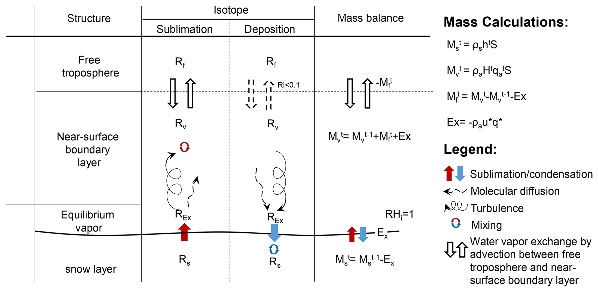
Figure 1 Schematic diagram of the box model used in this study. Please note that the dotted arrows between the free atmosphere and the boundary layer indicate that exchange can only take place under the condition that the Richardson number (Ri) is less than 0.1.

The atmosphere–snow water vapor exchange consists of two processes: sublimation and deposition (Fig. 1). During sublimation, water vapor is released from snow, transported into the atmospheric layer via turbulent mixing and molecular diffusion, and immediately mixed with the water vapor already in the boundary layer. During deposition, water vapor is influenced by aerodynamic resistance from turbulence and molecular diffusion, and the deposit is mixed with the surface snow layer. While water vapor transportation at the atmosphere–snow interface relies on two different diffusion pathways, turbulence plays a more crucial role in mass and energy exchanges (Brun et al., 2011; Vignon et al., 2017).

In the box model, atmosphere–snow water vapor exchange flux is calculated by turbulent quantities at each time step of 1 h, as detailed in Sect. 2.1.1. Based on atmosphere–snow water vapor exchange flux parameterization, the model further calculates temporal variations in snow and water vapor isotopic compositions according to isotopic mass balance (detailed in Sect. 2.1.2).

Model inputs mainly include meteorological conditions, e.g., air temperature (T_a), surface temperature (T_s), humidity (relative humidity, RH_w, or specific humidity, q_a)), and wind speed (u_a). Additional model inputs include the mixing-layer height (H₀), snow layer thickness (h₀), and the initial isotopic values, i.e., the snow isotopic composition (δ_s0), water vapor isotopic composition in the boundary layer (δ_v0), and water vapor isotopic composition in the free atmosphere (δ_f0).

2.1.1 Atmosphere–snow water vapor exchange flux parameterization

We used the bulk aerodynamic method and Monin–Obukhov similarity theory (Monin and Obukhov, 1954) to estimate turbulent fluxes. This approach calculates the net effects of sublimation and deposition at each time step using meteorological data, avoiding the parameterization of the individual fluxes of sublimation and deposition.

The bulk aerodynamic method estimates the atmosphere–snow water vapor exchange flux (Ex) through calculation of latent heat (LE) between the surface and one reference height (z) in the boundary layer (Berkowicz and Prahm, 1982). The expression is as follows:

$$\begin{array}{}\text{(1)}& \text{Ex}=\text{LE}/L_{\mathrm{s}}=-{\mathit{\rho }}_{\mathrm{a}}{u}^{\ast }{q}^{\ast },\end{array}$$

where ρ_a is the dry-air density varying with the observed air temperature (T_a) and pressure (P_a), L_s is the sublimation heat constant, and u^∗ and q^∗ are the friction velocity and specific humidity turbulence scale, respectively. u^∗ and q^∗ are defined as

$$\begin{array}{}\text{(2)}& {\displaystyle }{u}^{\ast }={\displaystyle \frac{k{u}_{\mathrm{a}}}{\log \left(\frac{z}{z_{\mathrm{0}}}\right)-{\mathrm{\Psi }}_{\mathrm{M}}\left(\frac{z}{L}\right)}}\text{(3)}& {\displaystyle }{q}^{\ast }={\displaystyle \frac{k(q_{\mathrm{a}}-q_{\mathrm{0}})}{\log \left(\frac{z}{z_{\mathrm{0}}}\right)-{\mathrm{\Psi }}_{\mathrm{M}}\left(\frac{z}{L}\right)}},\end{array}$$

where k denotes the von Kármán constant, u_a is the wind speed at the reference height in the boundary layer (z=4 m), q₀ is the saturated specific humidity at the snow surface derived from the Clausius–Clapeyron equation, q_a is the specific humidity that can be estimated from the observed relative humidity over the ice surface (RH_i) once the saturated specific humidity at the reference height (q_s) is known from the August–Roche–Magnus Formula at a given temperature (T_a), z₀ represents the surface roughness length for humidity exchange, and Ψ_M is the diabatic correction term with respect to the ratio of the reference layer height (z) and Monin–Obukhov length (L). L is defined as

$$\begin{array}{}\text{(4)}& L={\displaystyle \frac{\stackrel{\mathrm{‾}}{\mathit{\theta }}}{g}}{\displaystyle \frac{u_{\ast }^{\mathrm{2}}}{k{\mathit{\theta }}_{\ast }}},\end{array}$$

where $\stackrel{\mathrm{‾}}{\mathit{\theta }}$ is the mean potential temperature between the snow surface (θ₀) and the reference height in the boundary layer (θ_a), g is the gravitational acceleration, and u^∗ and θ^∗ are the friction velocity and temperature turbulence scale, respectively. The θ^∗ is analogous to u^∗ and q^∗, using θ_a, z₀, and $z/L$:

$$\begin{array}{}\text{(5)}& {\mathit{\theta }}^{\ast }={\displaystyle \frac{k({\mathit{\theta }}_{\mathrm{a}}-{\mathit{\theta }}_{\mathrm{0}})}{\log \left(\frac{z}{z_{\mathrm{0}}}\right)-{\mathrm{\Psi }}_{\mathrm{M}}\left(\frac{z}{L}\right)}}.\end{array}$$

In Eqs. (2), (3), and (5), z₀ can be estimated using least-squares fitting with the observed wind speed at three different heights under neutral atmospheric stratification. The Ψ_M is calculated for stable, unstable, and neutral boundary layers using the functions taken from Louis (1979). The determination of atmospheric stability depends on the Richardson number (Ri), which is defined as follows:

$$\begin{array}{}\text{(6)}& \mathit{Ri}={\displaystyle \frac{g}{{\mathit{\theta }}_z}}{\displaystyle \frac{z\mathrm{\Delta }\mathit{\theta }}{u_z^{\mathrm{2}}}}.\end{array}$$

Based on Eqs. (1)–(6), the atmosphere–snow water vapor exchange flux, Ex, can be calculated in the model with appropriate inputs. A positive value of Ex represents net sublimation (i.e., sublimation > deposition), while a negative value of Ex corresponds to net deposition (i.e., sublimation < deposition).

2.1.2 Isotopic mass balance

Assuming that the snow reservoir is influenced only by atmosphere–snow water vapor exchange (Fig. 1), temporal variations in snow mass per unit of surface area (S) can be expressed as

$$\begin{array}{}\text{(7)}& M_{\mathrm{s}}^t=M_{\mathrm{s}}^{t-\mathrm{1}}-\text{Ex},\end{array}$$

where Ex is the exchange flux as calculated in the previous section, M_s is the mass of the defined surface snow, and the superscript t denotes time. From Eq. (7), M_s at time t can be calculated from the initial snow masses (i.e., masses at t=0) and the accumulated Ex at time t. In the model, M_s at t=0 relies on the initial snow height (h₀) and snow density (ρ_s). The water vapor mass in the boundary layer (M_v) at time t and the unit area (S) can be computed from the initial boundary height (H₀), dry air density (ρ_a), and specific humidity (q_a) at the reference height in the boundary layer:

$$\begin{array}{}\text{(8)}& M_{\mathrm{v}}^t={\mathit{\rho }}_{\mathrm{a}}{H}_{\mathrm{0}}{q}_{\mathrm{a}}^{t}S,\end{array}$$

where q_a at time t can be determined by direct measurements or the observed relative humidity (RH_i). In Eq. (8), we neglect the temporal changes in the height of the boundary layer, given that the boundary heights in polar inland regions are relatively stable (Bonner et al., 2010; B. Ma et al., 2020). According to Eq. (8), the mass changes in the atmospheric boundary water vapor layer at each time interval are ${\mathit{\rho }}_{\mathrm{v}}{H}_{\mathrm{0}}(q_{\mathrm{a}}^t-q_{\mathrm{a}}^{t-\mathrm{1}}$). This quantity is influenced by atmosphere–snow water vapor exchange (Ex) and the water vapor exchange flux from the free atmosphere to the boundary layer (M_f). Thus, M_f at any time can be quantified as follows:

$$\begin{array}{}\text{(9)}& M_{\mathrm{f}}^t=M_{\mathrm{v}}^t-M_{\mathrm{v}}^{t-\mathrm{1}}-\text{Ex}={\mathit{\rho }}_{\mathrm{v}}{H}_{\mathrm{0}}(q_{\mathrm{a}}^t-q_{\mathrm{a}}^{t-\mathrm{1}})-\text{Ex}.\end{array}$$

Note that the exchange between the boundary layer and the free atmosphere can occur under unstable conditions or weakly stable conditions (Zilitinkevich and Esau, 2007). In the model, we hold that M_f can contribute to the atmospheric boundary water vapor reservoir when the Richardson number is less than 0.1 (i.e., including weakly stable conditions in addition to unstable conditions).

Based on the calculation of mass changes in the three reservoirs (Eqs. 7–9), the isotopic mass equations are

$$\begin{array}{}\text{(10a)}& {\displaystyle }{M}_{\mathrm{s}}^t{R}_{\mathrm{s}}^t=M_{\mathrm{s}}^{t-\mathrm{1}}{R}_{\mathrm{s}}^{t-\mathrm{1}}-R_{\text{Ex}}^t\times \text{Ex}\text{(10b)}& {\displaystyle }{M}_{\mathrm{v}}^t{R}_{\mathrm{v}}^t=M_{\mathrm{v}}^{t-\mathrm{1}}{R}_{\mathrm{v}}^{t-\mathrm{1}}+R_{\text{Ex}}^t\times \text{Ex}+R_{\mathrm{f}}^t\times M_{\mathrm{f}}^t,\end{array}$$

where R_s, R_v, R_f, and R_Ex represent the ratios of heavy isotopes (¹⁸O and D) and light isotopes (¹⁶O and H) in the snow layer, atmospheric boundary layer, free-atmospheric layer, and exchange flux, respectively.

The calculation of R_Ex differs between the sublimation-dominated (i.e., net sublimation) period and deposition-dominated (i.e., net deposition) period. For the sublimation-dominated phase (Ex>0), kinetic fractionation is assumed to occur when the sub-saturation condition is considered. The isotopic composition of the sublimated vapor is calculated from Merlivat and Jouzel (1979), combining R_s, R_v, the diffusion coefficient (k^′), the equilibrium coefficient (α_e), and the relative humidity of the air with respect to the surface temperature (h) as follows:

$$\begin{array}{}\text{(11)}& R_{\text{Ex}}^t={\displaystyle \frac{\mathrm{1}-k^{\prime }}{\mathrm{1}-h}}\left({\displaystyle \frac{R_{\mathrm{s}}^t}{{\mathit{\alpha }}_{\mathrm{e}}}}-h\times R_{\mathrm{v}}^t\right).\end{array}$$

The isotopic composition of the condensed vapor (Ex<0) is in equilibrium with that of the water vapor above −20 °C. However, kinetic fractionation will also occur due to vapor supersaturation over ice on the eastern Antarctic Plateau. This effect can reduce the effective fractionation of water isotopes. Therefore, the equilibrium coefficient (α_e) is replaced by the effective fractionation coefficient (α_f) when calculating the R_Ex of condensed vapor. α_f is defined as the product of the kinetic fractionation coefficient (α_k) and α_e. The R_Ex of condensed vapor is thus expressed as

$$\begin{array}{}\text{(12)}& R_{\text{Ex}}^t={\mathit{\alpha }}_{\mathrm{f}}(R_{\mathrm{v}}^t+\mathrm{1})-\mathrm{1}.\end{array}$$

α_e with respect to ice is given by Ellehoj et al. (2013) as a function of temperature (Eq. 13).

$$\begin{array}{}\text{(13a)}& {\displaystyle }{\mathit{\alpha }}_{\mathrm{e}}^{{}^{\mathrm{18}}\mathrm{O}}=\exp \left(\mathrm{0.0831}-{\displaystyle \frac{\mathrm{49.192}}{T}}+{\displaystyle \frac{\mathrm{8312.5}}{T^{\mathrm{2}}}}\right)\text{(13b)}& {\displaystyle }{\mathit{\alpha }}_{\mathrm{e}}^{\mathrm{D}}=\exp \left(\mathrm{0.2133}-{\displaystyle \frac{\mathrm{203.10}}{T}}+{\displaystyle \frac{\mathrm{48}\mathrm{888}}{T^{\mathrm{2}}}}\right)\end{array}$$

α_f is deduced from α_e as follows

$$\begin{array}{}\text{(14)}& {\mathit{\alpha }}_{\mathrm{f}}={\mathit{\alpha }}_{\mathrm{e}}{\displaystyle \frac{{\text{RH}}_{\mathrm{i}}}{\mathrm{1}+{\mathit{\alpha }}_{\mathrm{e}}({\text{RH}}_{\mathrm{i}}-\mathrm{1})\left(\frac{D_{\mathrm{i}}}{D_{\mathrm{i}}^{\prime }}\right)}},\end{array}$$

where D_i is the diffusivity of the water molecule and $D_{\mathrm{i}}^{\prime }$ is the same as D_i but for heavy isotopes. The ratios of $D_{\mathrm{i}}/D_{\mathrm{i}}^{\prime }$ are given by Jouzel and Merlivat (1984), with values of 1.0285 for ¹⁸O and 1.0251 for D.

The key variables in the model are summarized and listed in Table S1 in the Supplement.

2.2 Model simulations

We first used the abovementioned model to simulate atmosphere–snow water vapor exchange and the associated isotope effects at Dome C (75.10° S, 123.33° E; 3233 m a.s.l.), where diurnal variations in water vapor isotopic compositions as well as surface snow water isotopes are available from observations (Casado et al., 2016; Touzeau et al., 2016). We then applied the model to Dome A conditions to investigate the isotopic effects due to atmosphere–snow water vapor exchange at diurnal scales. The initial model values, including mixing-layer height (H₀), snow layer height (h₀), snow isotopic composition (δs₀), water vapor isotopic composition in the boundary layer (δv₀), water vapor isotopic composition in the free-atmosphere layer (δf₀), and snow density (ρ_s) are listed in Table 1. These values were justified according to the conditions discussed in the following sections.

Table 1 Key initial values for diurnal simulations.

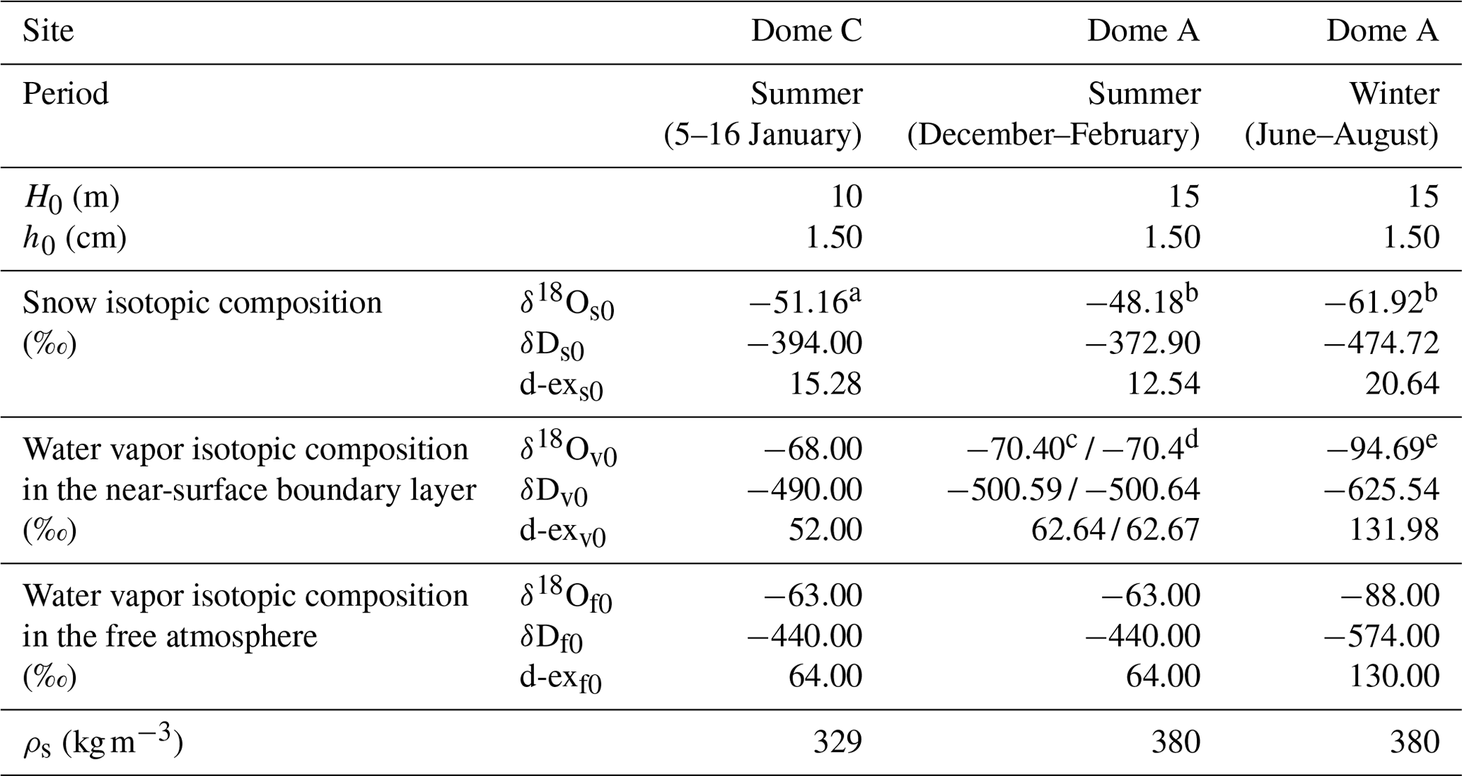
^a, b Observations for surface snow isotopes and calculations for fresh snow isotopes, respectively. ^c, d Values correspond to clear-sky and highly cloudy conditions, respectively. ^e Some of the winter conditions were set the same as those in summer (see details in Sect. 2.2.3).

2.2.1 Diurnal simulations under Dome C conditions

At Dome C, previous observations revealed a clear diurnal cycle of water vapor isotopic composition from 5 to 16 January 2015 (Casado et al., 2016). This diurnal cycle was attributed to the effects of atmosphere–snow water vapor exchange under clear-sky conditions (Casado et al., 2018). To compare the modeled results with the observations, we performed a continuous simulation using observed meteorological data over the same period (11 d). Meteorological parameters (e.g., temperature, humidity, and wind speed) during the observed period were downloaded from the CALibration and VAlidation of meteorological and climate models and satellite retrievals (CALVA) program (Genthon et al., 2010). The surface snow temperature (T_s) data are available in a previous publication (Casado et al., 2016). The boundary height, H₀, was determined by Doppler sodar measurements from an on-site iron tower at Dome C (Vignon et al., 2017). The surface snow layer height, h₀, was set to be the thickness of surface snow collected (i.e., 1.5 cm) for isotopic composition analysis at this site (Casado et al., 2018). The initial vapor isotopic compositions in the boundary layer, δv₀, were set as the observations of water vapor δ¹⁸O, δD, and deuterium excess (d-excess) at the beginning of the modeling period during the 2014/15 field season (Casado et al., 2016), while snow isotopes, δs₀, were set as the mean isotopic values of summer surface snow samples (Casado et al., 2018). The water vapor isotopic composition in the free atmosphere layer (δf₀) was not reported at this site. Here we expect that δf₀ is greater than δv₀. Although there are currently no vertical observations of water vapor isotopic composition in Antarctica, vertical isotopic profiles (δ¹⁸O) observed at Summit Camp, Greenland, have indicated that the isotopic composition of water vapor in the free atmosphere is slightly higher than that within the boundary layer (Berkelhammer et al., 2016). In order to explain the water vapor and snow isotope observations at Dome C, Casado et al. (2018) assumed that the contribution from the free atmosphere can increase the ratio of ${{\mathrm{H}}_{\mathrm{2}}}^{\mathrm{18}}\mathrm{O}$ molecules in the boundary layer (Casado et al., 2018) and set δf₀ as the highest observed value of water vapor isotopic composition at Dome C. Note that δf₀ was a constant value for the simplicity of model calculations. The density of the topmost 5 cm of surface snow (ρ_s) was reported by Champollion et al. (2019).

2.2.2 Simulations under Dome A summer conditions

Previous studies have shown that a diurnal cycle clearly occurs in surface snow and water vapor isotopic compositions during clear-sky days, whereas this feature is not significant in highly cloudy periods (Casado et al., 2016; Ritter et al., 2016; Hughes et al., 2021). Clouds play an important role in modulating atmospheric thermal and dynamic conditions (Haynes et al., 2013), and cloudy conditions may also mean more moisture present in the atmosphere. Under cloudy conditions, extra moisture and downward radiation from clouds likely disturb local temperature and humidity variabilities, resulting in smaller differences between day and night atmosphere–snow water vapor exchange, and thus the isotopic effects are less pronounced. Therefore, in the model simulations for Dome A summer conditions, we not only simulated continuous changes in surface snow and water vapor isotopic composition over a multiday timescale but also incorporated two representative scenarios (i.e., cloudy vs. clear-sky conditions) to ensure a rigorous assessment of the isotopic variations associated with atmosphere–snow water vapor exchange processes.

The simulations with continuous meteorological input were conducted without considering the influence of clouds. The selected period for summer simulations was from 5 to 16 January for each year from 2006 to 2011 (with the exception of 2005 for which data were not available). The model was thus run for 11 d each year, consistent with the Dome C simulations. By averaging the six simulated results obtained from the simulations, we were able to estimate the continuous changes in water vapor and snow isotopic composition. This approach allowed for a more robust analysis of the simulated data and enabled a direct comparison of the results across different cases (results shown in Sect. 3.2.4 and Fig. 7).

The hourly averages of total cloud cover (Tcc) were used to select days with clear-sky and highly cloudy conditions. These data were retrieved from the ERA5 reanalysis dataset, with a spatial resolution of 1.25°×1.25°. Based on previous studies, the classification criteria are as follows: Tcc≤0.3 for clear-sky conditions and Tcc≥0.8 for highly cloudy conditions (Qian et al., 2012). Following this criterion, we selected 20 clear-sky days during the summer period (December to February) of 2005–2011. Then, the hourly meteorological data from those selected days were stacked to create a representative cycle for model initialization. For highly cloudy conditions, a stack of 102 diurnal cycles of meteorological variables was also produced for modeling at the diurnal scale.

Meteorological data were obtained from an automatic weather station (AWS) installed near the summit of Dome A. The hourly surface air pressure; air temperature at heights of 1, 2, and 4 m; relative humidity at 4 m; wind speed at heights of 1, 2, and 4 m; and wind direction are available for the period of 2005–2011 (Ma et al., 2010; Ding et al., 2022). The surface snow temperature (T_s) observations were not available at Dome A. Thus, we performed T_s calculations based on the method from Brun et al. (2011). The equation for T_s calculation is shown as follows:

$$\begin{array}{}\text{(15)}& T_{\mathrm{s}}={\left({\displaystyle \frac{{\text{LW}}_{\text{up}}+(\mathit{ϵ}-\mathrm{1}){\text{LW}}_{\text{dn}}}{\mathit{ϵ}\mathit{\sigma }}}\right)}^{\mathrm{0.25}},\end{array}$$

where σ is the Stefan–Boltzmann constant, ϵ is the snow emissivity (0.93), and LW_dn and LW_up are the downward and upward longwave radiative fluxes, respectively. The hourly longwave radiative flux data were retrieved from the ERA5 reanalysis dataset.

The stacked hourly mean values of the meteorological conditions at Dome A are shown in Fig. 2a. During clear-sky conditions, the air temperature at the 4 m level (T_a) shows a diurnal cycle with an amplitude of 10 °C and an average of −31 °C. The diurnal T_s follows a similar pattern to that of T_a, varying between −39 and −28 °C. The ranges of diurnal cycles for specific humidity (q_a) and relative humidity (RH_i) are 1.8–$\mathrm{3.7}\times {\mathrm{10}}^{-\mathrm{4}}$ kg kg⁻¹ and 66 %–130 %, respectively. q_a is also parallel to T_a, whereas RH_i shows an opposite trend. In contrast to temperature and humidity, the daily air pressure near the surface is stable (∼584 hPa). The wind speed (u_a) and latent heat flux reached daily maxima of 3.0 m s⁻¹ and 3.3 W m⁻², respectively, at 10:00 UTC, coinciding with the peaks in T_a, T_s, and q_a at the diurnal scale. Under highly cloudy conditions, the latent heat exhibits less variability, yet q_a and u_a display greater diurnal variations (Fig. 2b).

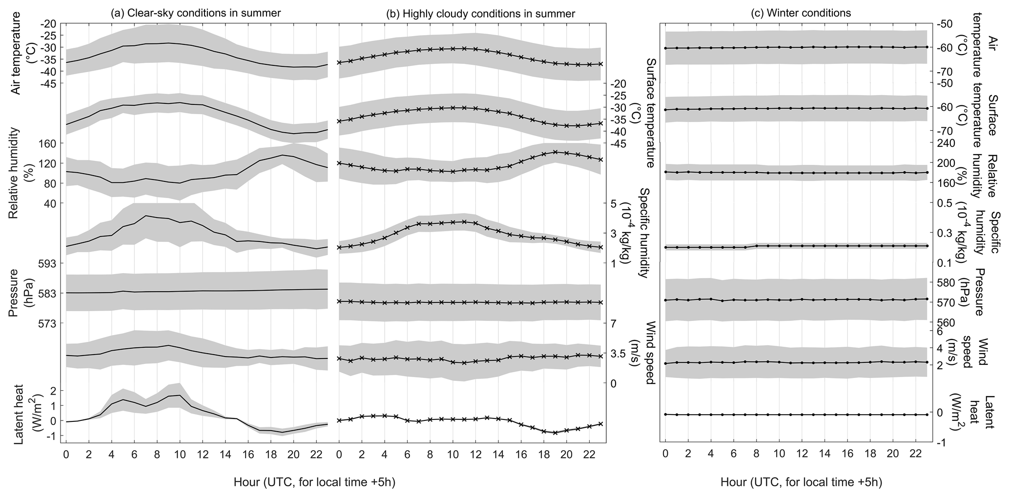
Figure 2 Stacks of diurnal cycles of meteorological parameters and the calculated latent heat under summer clear-sky conditions (a), summer highly cloudy conditions (b), and winter conditions (c) at Dome A. The hourly air temperature, relative humidity, air pressure, and wind speed data were averaged from the AWS observations on the selected days. The diurnal variations in the other three parameters were calculated based on hourly observations. In each panel, the solid line with marks represents the average and the gray shadow represents the standard deviation (±1σ).

The initial model values of H₀, h₀, δs₀, δv₀, and ρ_s for the Dome A simulations are listed in Table 1. H₀ was estimated as the median thickness of the boundary layer (15 m) based on sonic radar and visual observations of the angular size of stellar images during summer (Bonner et al., 2010; B. Ma et al., 2020). The surface snow thickness, h₀, was set to 1.5 cm according to summer snow accumulation at Dome A (calculated from the annual mean snow accumulation of 18–23 mm yr⁻¹). δs₀ values were obtained from the average precipitation isotopic composition measurements during the 2009/10 field season at Dome A (Pang et al., 2019). The δv₀ can be calculated from δs₀ assuming atmosphere-snow equilibrium and using the equilibrium fractionation coefficient at the surface temperature of the beginning of the diurnal cycle. δf₀ was set equal to the value at Dome C, since there are no measurements available from Dome A. The ρ_s in Table 1 was from the measurements taken during the 2014/15 field season (T. Ma et al., 2020).

2.2.3 Simulations under Dome A winter conditions

Given the different meteorological conditions in winter compared to summer, the degree of atmosphere–snow water vapor exchange and the associated isotope effects could be different. Therefore, we also conducted multiday and diurnal simulations for winter at Dome A, similar to the summer simulations. This may shed light on assessments of the effects of atmosphere–snow water vapor exchange on seasonal and annual scales.

Winter simulations that incorporated continuous meteorological data were executed for a duration of 11 d, spanning 5 to 16 July for each year between 2006 and 2011. This enabled the acquisition of six simulated results, which were subsequently averaged to provide a comprehensive understanding of the continuous changes in water vapor and snow isotopic composition over a multiday timescale.

The stacked hourly mean values of winter meteorological conditions at Dome A were extracted in the same way as we did for the summer conditions. As shown in Fig. 2c, the average temperature, specific humidity, and atmospheric pressure are lower than those in summer, but the relative humidity increases during winter. These changes result in the negative values of latent heat flux during winter. In addition, the winter meteorological parameters and latent heat flux do not show any apparent diurnal variations.

The initial model values for the winter simulations are also listed in Table 1. The initial value of the snow isotopic composition ($\mathit{\delta }{{}^{\mathrm{18}}\mathrm{O}}_{\text{s0}}$) is the average of the precipitation isotopic composition at the starting month for the winter season. Due to the lack of observations, $\mathit{\delta }{{}^{\mathrm{18}}\mathrm{O}}_{\text{s0}}$ was estimated from the monthly mean temperature and the δ–T slopes in non-summer seasons (0.64 ± 0.02) according to the compiled data from Pang et al. (2019). We also further evaluated these estimations of $\mathit{\delta }{{}^{\mathrm{18}}\mathrm{O}}_{\text{s0}}$ by a comparison with snowfall δ¹⁸O modeled using the water-isotope-enabled ECHAM5 general circulation model (ECHAM5-wiso; Werner et al., 2011). The results of the two methods agree with each other (Sect. S3 in the Supplement), suggesting that $\mathit{\delta }{{}^{\mathrm{18}}\mathrm{O}}_{\text{s0}}$ estimation using the regression line is reliable. The initial value for the water vapor isotopic composition ($\mathit{\delta }{{}^{\mathrm{18}}\mathrm{O}}_{\text{v0}}$) was also estimated assuming isotope equilibrium with $\mathit{\delta }{{}^{\mathrm{18}}\mathrm{O}}_{\text{s0}}$. δf₀ was set to the calculated $\mathit{\delta }{{}^{\mathrm{18}}\mathrm{O}}_{\text{v0}}$ using $\mathit{\delta }{{}^{\mathrm{18}}\mathrm{O}}_{\text{s0}}$ and the highest temperature observed in winter during the studied period. h₀ is kept the same as that in summer to simplify the calculations. The median H₀ at Dome A varies little throughout most of the year according to Bonner et al. (2010) and B. Ma et al. (2020), so in the model we used the same H₀ in winter as that in summer. ρ_s is the annual mean snow density based on measurements (T. Ma et al., 2020), and we did not consider seasonal variations to simplify the calculations.

2.2.4 Sensitivity simulations

Changes in initial parameters could influence the isotopic effects of atmosphere–snow water vapor exchange. For example, previous field experiments have indicated that isotopic enrichment caused by atmosphere–snow water vapor exchange tends to decrease as snow thickness increases (Hughes et al., 2021). Ritter et al. (2016) noted that diurnal variations in water vapor isotopic composition decrease as the mixing-layer height (i.e., H₀) increases. These previous findings motivate us to investigate the sensitivity of the modeled results to these boundary conditions and initial values.

The sensitivity tests included three groups of comparative experiments for the Dome A site and were run for a 24 h period under summer clear-sky conditions. The first group focuses on the sensitivity of surface and water vapor δ¹⁸O to varying h₀ and H₀. In the experiment, we vary h₀ between 0.1 and 3.0 cm (Ritter et al., 2016; Hughes et al., 2021) and H₀ from 1 to 100 m (Bonner et al., 2010; Ritter et al., 2016). The second group is designed to investigate how the uncertainties in $\mathit{\delta }{{}^{\mathrm{18}}\mathrm{O}}_{\text{s0}}$ and $\mathit{\delta }{{}^{\mathrm{18}}\mathrm{O}}_{\text{v0}}$ influence the isotopic effects of atmosphere–snow water vapor exchange, especially when $\mathit{\delta }{{}^{\mathrm{18}}\mathrm{O}}_{\text{s0}}$ and $\mathit{\delta }{{}^{\mathrm{18}}\mathrm{O}}_{\text{v0}}$ are not in equilibrium. We varied $\mathit{\delta }{{}^{\mathrm{18}}\mathrm{O}}_{\text{s0}}$ and $\mathit{\delta }{{}^{\mathrm{18}}\mathrm{O}}_{\text{v0}}$ from −53 ‰ to −43 ‰ (the range of summer precipitation δ¹⁸O at Dome A; Pang et al., 2019) and −85 ‰ to −55 ‰, respectively. The range of $\mathit{\delta }{{}^{\mathrm{18}}\mathrm{O}}_{\text{v0}}$ is estimated from $\mathit{\delta }{{}^{\mathrm{18}}\mathrm{O}}_{\text{s0}}$ and the equilibrium fractionation coefficient under summer conditions, and $\mathit{\delta }{{}^{\mathrm{18}}\mathrm{O}}_{\text{s0}}$ and $\mathit{\delta }{{}^{\mathrm{18}}\mathrm{O}}_{\text{v0}}$ in thermodynamic imbalance are included. In the third group, $\mathit{\delta }{{}^{\mathrm{18}}\mathrm{O}}_{\text{f0}}$ and snow density were varied to test their influence on the diurnal changes in surface snow and water vapor δ¹⁸O, respectively. The selection of −68 ‰ to −58 ‰ for the $\mathit{\delta }{{}^{\mathrm{18}}\mathrm{O}}_{\text{f0}}$ range refers to the summer observations of water vapor isotopic composition at Dome C (Casado et al., 2016). According to field observations at Dome A and other interior domes (Laepple et al., 2018), the range of snow density was set to 300–400 kg m⁻³ for sensitivity simulations. Note that the isotope effects are greater in summer than in winter; we only used summer conditions and values to illustrate the sensitivity of the modeled results to these parameters.

3 Results

3.1 Modeled diurnal and multiday variations at Dome C

On the diurnal scale at Dome C, the modeled water vapor δ¹⁸O increases from −68 ‰ at 00:00 UTC to −66 ‰ at 09:00 UTC and then decreases to −75 ‰ at 16:00 UTC (Fig. 3a). The diurnal patterns in water vapor δD are similar to those in water vapor δ¹⁸O, and their max–min difference is ∼54 ‰ (Fig. 3b). The water vapor d-excess, defined as d-excess (‰) $\equiv \mathit{\delta }\mathrm{D}-\mathrm{8}\times \mathit{\delta }{}^{\mathrm{18}}\mathrm{O}$ (Dansgaard, 1964), varies between 52 ‰ and 72 ‰ during the 24 h period (Fig. 3c). Its diurnal pattern is opposite to that of δ¹⁸O and δD. The modeled snow δ¹⁸O and δD also exhibit a diurnal pattern where higher values occur during the warming phase and lower values occur during the cooling phase (Fig. 3d). The diurnal range of simulated snow δ¹⁸O is ∼1.5 ‰ on average, but its value is close to that of the observations (2.0 ‰) during a typical frost event from 6 to 7 January 2015. In addition, the diurnal variations in snow d-excess are opposite to those in snow δ¹⁸O and δD, similar to the relationship between vapor δ¹⁸O and d-excess. Overall, the modeled diurnal variations in vapor δ¹⁸O and δD capture the observations well, while their magnitudes are slightly different from those in the observations.

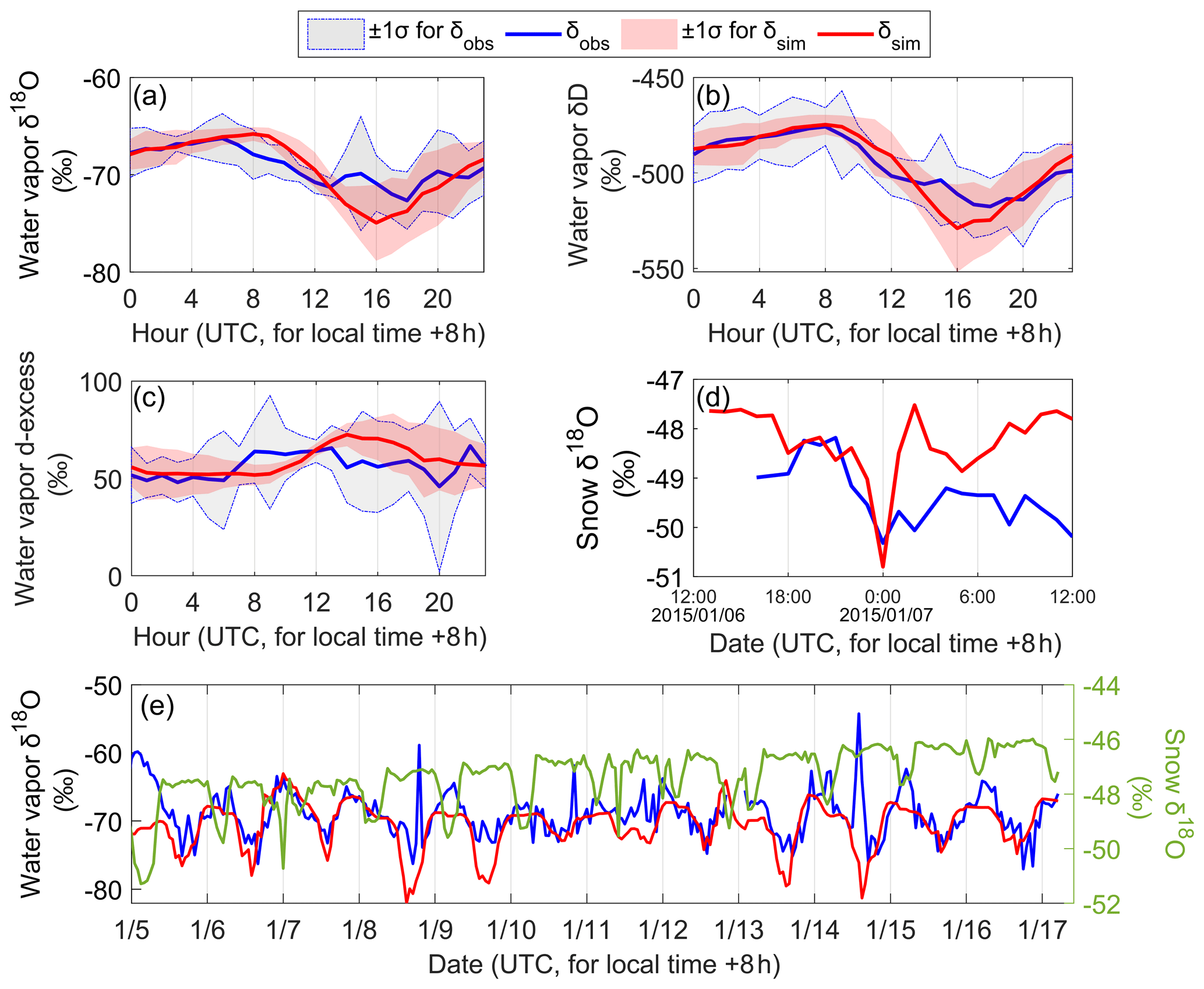
Figure 3 Modeled variations in water vapor and snow isotopic compositions at Dome C along with the observations. (a) Diurnal variations in water vapor δ¹⁸O, (b) diurnal variations in water vapor δD, (c) diurnal variations in water vapor d-excess, (d) diurnal variations in snow isotopes during 6–7 January 2015, and (e) continuous variations in water vapor and snow δ¹⁸O during 5–16 January 2015. In all panels, the solid blue line represents the observations (δ_obs), with the light-gray shaded area as the uncertainties (±1σ). The solid red line and the light-red shaded area depict the simulation (δ_sim) and corresponding uncertainties (±1σ). In panel (e), the solid green line represents the modeled snow δ¹⁸O. Note that snow δ¹⁸O observations at Dome C are available only from 6 to 7 January 2015 (Casado et al., 2018). The method for uncertainty estimation can be found in Sect. S2 in the Supplement.

The continuous simulations at the multiday scale are shown in Fig. 3e. The simulated water vapor δ¹⁸O exhibits periodic changes on the diurnal scale, but its daily mean value remains unchanged over the course of the simulation. This trend is consistent with the observations reported by Casado et al. (2016), as evidenced by a high correlation coefficient (R>0.6). The snow δ¹⁸O values display a noticeable enrichment trend compared to their initial state, which is different from that of the water vapor δ¹⁸O.

3.2 Modeled results at Dome A

3.2.1 Diurnal variations under summer clear-sky conditions

At Dome A, the Richardson number (Ri) varies between −0.01 and 0.02 during the 24 h period (Fig. 4a). The friction velocity of water molecules (u^∗) ranges from 0.11 to 0.19 m s⁻¹, with a mean value of 0.14 m s⁻¹ (Fig. 4b). The atmosphere–snow water vapor exchange flux (Ex) calculated from Ri and u^∗ varies in parallel with temperature (Fig. 4c). In general, negative Ri values represent relatively unstable atmospheric conditions, which correspond to the phase of sublimation (i.e., net vapor flux from snow to the atmosphere; Fig. 4c). In contrast, Ri appears to be positive during most of the cooling phase (i.e., the net vapor flux from the atmosphere to snow; Fig. 4c), suggesting stable atmospheric conditions.

Figure 4d–f displays the modeled surface snow and water vapor isotopic compositions and the uncertainties. All the isotopes display apparent diurnal cycles. In particular, water vapor δ¹⁸O and δD indicate enrichments in the sublimation period, followed by depletions during the rest of the day when condensation (vapor deposition) dominates (Fig. 4d and e). The snow δ¹⁸O and δD values exhibit similar but somewhat opposite patterns within 24 h (Fig. 4d and e). The diurnal pattern of d-excess is opposite to that of δ¹⁸O and δD in snow and vapor (Fig. 4f). Overall, the diurnal patterns of snow and water vapor isotopes at Dome A are similar to those at Dome C during summer cloudless conditions.

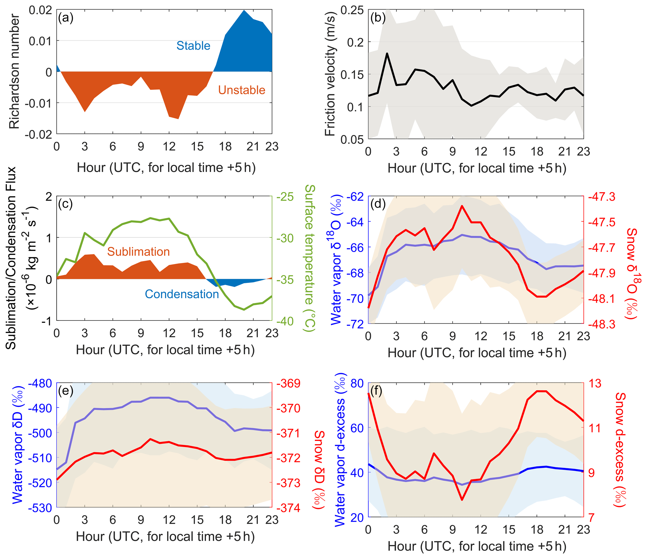
Figure 4 The simulated hourly mean vapor exchange flux and variations in atmospheric water vapor and snow isotopes under summer clear-sky conditions at Dome A: (a) Richardson number, (b) friction velocity, (c) vapor exchange flux, (d) snow and water vapor δ¹⁸O, (e) snow and water vapor δD, and (f) snow and water vapor d-excess. The uncertainties for each variable are displayed by shaded areas in each panel.

The magnitudes of the diurnal range in water vapor isotopic composition are 4.8 ‰ for δ¹⁸O, 29 ‰ for δD, and 9.3 ‰ for d-excess. In comparison, the modeled diurnal isotope variations in surface snow are much smaller with magnitudes of 0.80 ‰ for δ¹⁸O, 1.6 ‰ for δD, and 4.9 ‰ for d-excess. In addition, after 24 h of model operation, the water vapor δ¹⁸O, δD, and d-excess increase by 2.4 ‰, 16 ‰, and 3.1 ‰, respectively (Fig. 4d–f). Moreover, after 24 h, the snow isotopic compositions display enrichments of 0.29 ‰ for δ¹⁸O and 1.1 ‰ for δD and a depletion of 1.3 ‰ for d-excess.

3.2.2 Diurnal variations under highly cloudy summer conditions

Under highly cloudy conditions, the Richardson number (Ri) is almost neutral or unstable at the diurnal scale (Fig. 5a). The friction velocity (u^∗) exhibits a diurnal cycle varying between 0.11 and 0.13 m s⁻¹ (Fig. 5b), which is much smaller than that under clear-sky conditions. We also found a diurnal cycle in the atmosphere–snow water vapor exchange flux (Ex), as shown in Fig. 5c. Overall, the diurnal changes in u^∗, Ri, and Ex are less pronounced compared with those under clear-sky conditions.

Figure 5 Same as Fig. 4 but for Dome A under highly cloudy conditions in summer.

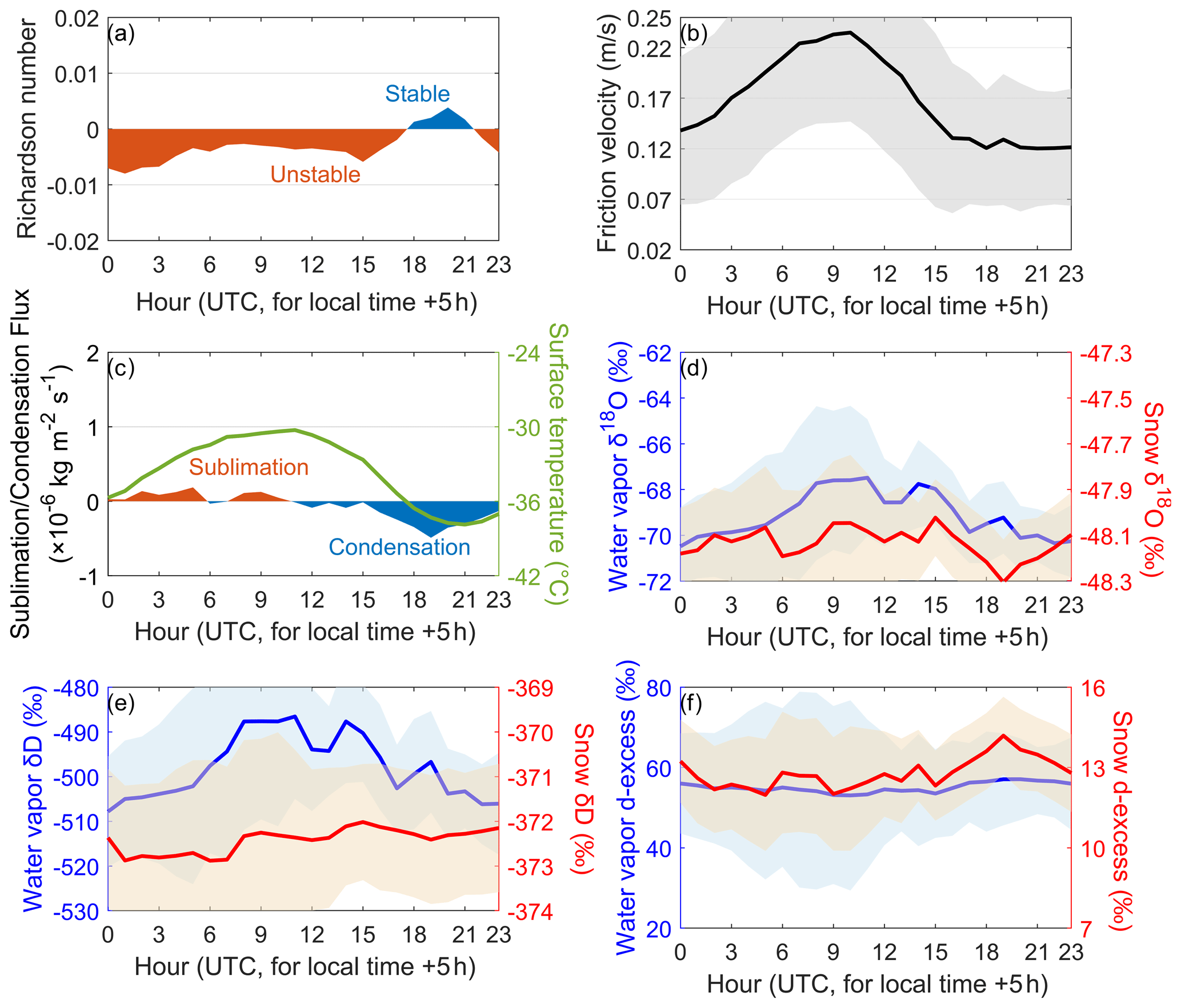
The diurnal cycle patterns in water and surface snow isotopic compositions are also apparent under cloudy conditions (Fig. 5d–f), but the magnitudes are smaller than those under clear-sky conditions. In particular, the diurnal peak-to-valley differences in water vapor isotopic compositions are 3.0 ‰ for δ¹⁸O, 21 ‰ for δD, and 4.0 ‰ for d-excess. The diurnal variations in the surface snow isotopic composition have a magnitude of 0.28 ‰ for δ¹⁸O, 0.87 ‰ for δD, and 2.2 ‰ for d-excess. In addition, after 24 h, snow water isotopes were enriched in the model, the same as in clear-sky conditions.

3.2.3 Diurnal variations under winter conditions

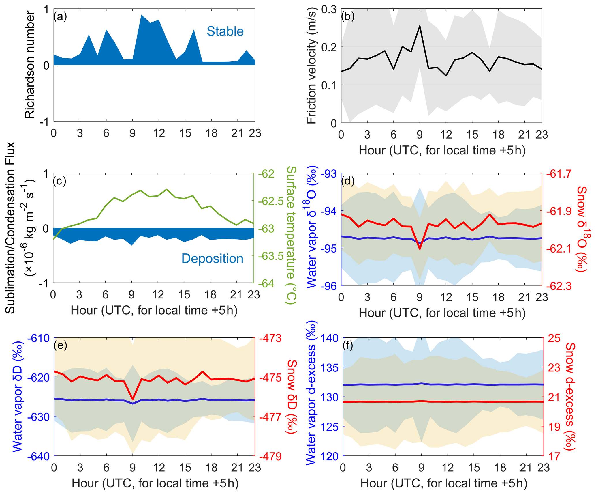
The winter simulation results are plotted in Fig. 6. Under winter conditions, the Richardson number (Ri) and the friction velocity (u^∗) remain stable over a full 24 h period (Fig. 6a and b). The atmosphere–snow water vapor exchange flux (Ex) shows negative values throughout 24 h (Fig. 6c), suggesting that sublimation does not occur under Dome A winter conditions. As a result, in contrast to the simulated results in summer, there are no significant diurnal variations in snow isotopes in winter, but the changes in water vapor isotopic composition in winter are comparable to those in summer. This can be associated with the almost-constant meteorological conditions and the relatively weak exchange between snow and atmospheric water vapor during a diurnal period, as displayed in Fig. 2c. In addition, because the isotopic composition of deposited vapor is much lower than that of surface snow, the winter snow layer experiences small but steady depletions in δ¹⁸O and δD (Fig. 6d and e). In contrast, snow d-excess becomes more enriched under the effects of the atmosphere–snow water vapor exchange flux (Fig. 6f). The water vapor isotopic composition also displays depletion because heavier isotopes tend to deposit faster.

Figure 6 Same as Fig. 4 but for Dome A under winter conditions.

3.2.4 Continuous changes at the multiday scale at Dome A

The continuous simulations presented in Fig. 7 reveal that the water vapor isotopic composition (δ¹⁸O) exhibits substantial interannual differences in absolute values, even during the same period (Fig. 7a and c). In addition, these simulations and their averages display distinct diurnal periodicity. On the multiday scale, the average water vapor δ¹⁸O values do not show a significant trend with increasing simulation time. Their values fluctuate around −72 ‰ in the summer and −105 ‰ in the winter. The diurnal cycles shown in the Dome A continuous simulations are consistent with the simulated results at Dome C.

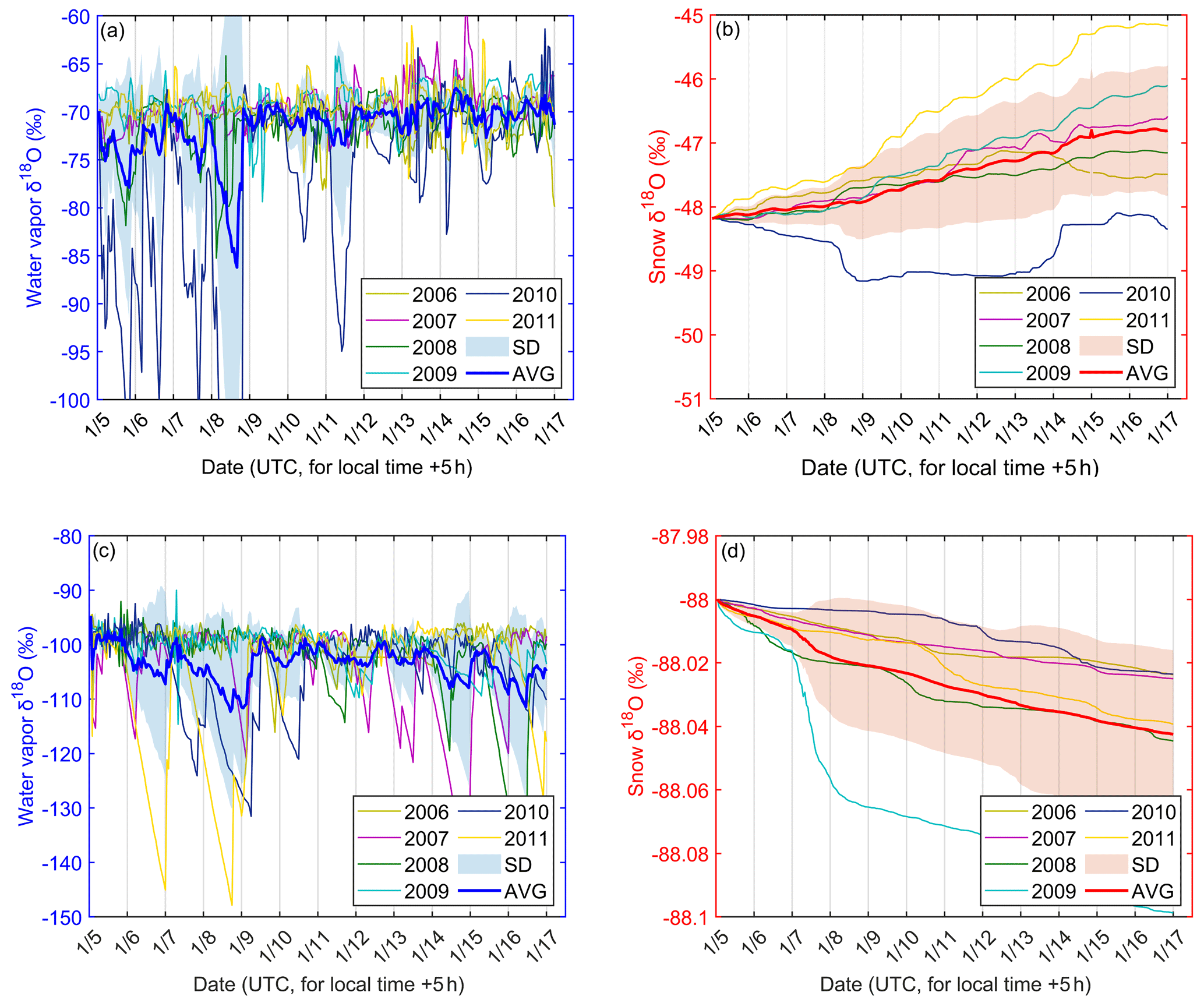
Figure 7 Continuous simulations of snow and water vapor isotopes at Dome A. Panels (a) and (b) represent summer simulations over an 11 d period (5–16 January 2006–2011), and panels (c) and (d) are the same as panels (a) and (b) but for wintertime (5–16 July 2006–2011). In all panels, the colored lines represent the simulated results of water vapor δ¹⁸O for each year during the simulation period. The bold lines and the light-blue/red shadows are the averages (AVGs) and standard deviations (SDs) of the δ¹⁸O simulations in each year, respectively.

The snow isotopic composition (δ¹⁸O) simulations in each year exhibit a striking similarity in their trends during the summer and winter seasons. Specifically, the snow δ¹⁸O values at the end of the simulation are consistently higher than the initial values during the summer (Fig. 7b). Conversely, a slightly negative trend can be observed in the winter simulations (Fig. 7d).

3.3 Sensitivity to model parameters

In the first group of sensitivity tests (Fig. 8a), the water vapor and snow isotopic composition displayed distinct patterns in response to variations in the snow depth (h₀) and the boundary layer height (H₀). The magnitude of the diurnal variations in water vapor δ¹⁸O ($\mathit{\delta }{{}^{\mathrm{18}}\mathrm{O}}_{\mathrm{v}}$) is highly influenced by H₀ but not by h₀. This finding aligns with previous calculations at Kohnen Station, which demonstrated a decrease in the magnitude of $\mathit{\delta }{{}^{\mathrm{18}}\mathrm{O}}_{\mathrm{v}}$ with increasing mixing-layer height (Ritter et al., 2016). On the other hand, the magnitude of diurnal variations in snow δ¹⁸O ($\mathit{\delta }{{}^{\mathrm{18}}\mathrm{O}}_{\mathrm{s}}$) exhibits a greater sensitivity to h₀ (Fig. 8b). This finding is consistent with field experiments showing that isotopic enrichment induced by atmosphere–snow water vapor exchange tends to decrease with increasing snow thickness (Hughes et al., 2021). Similar to the magnitude of $\mathit{\delta }{{}^{\mathrm{18}}\mathrm{O}}_{\mathrm{s}}$, the changes in $\mathit{\delta }{{}^{\mathrm{18}}\mathrm{O}}_{\mathrm{s}}$ after a diurnal cycle are more sensitive to h₀ (Fig. 8c).

In the second group of tests, where $\mathit{\delta }{{}^{\mathrm{18}}\mathrm{O}}_{\text{s0}}$ and $\mathit{\delta }{{}^{\mathrm{18}}\mathrm{O}}_{\text{v0}}$ vary, the magnitude of $\mathit{\delta }{{}^{\mathrm{18}}\mathrm{O}}_{\mathrm{v}}$ diurnal changes is more sensitive to $\mathit{\delta }{{}^{\mathrm{18}}\mathrm{O}}_{\text{v0}}$ than to $\mathit{\delta }{{}^{\mathrm{18}}\mathrm{O}}_{\text{s0}}$ (Fig. 8d). As $\mathit{\delta }{{}^{\mathrm{18}}\mathrm{O}}_{\text{s0}}$ decreases, the magnitude of $\mathit{\delta }{{}^{\mathrm{18}}\mathrm{O}}_{\mathrm{s}}$ diurnal changes increases, emphasizing the influence of $\mathit{\delta }{{}^{\mathrm{18}}\mathrm{O}}_{\text{s0}}$ on snow isotopic variations (<0.05 ‰ in Fig. 8e). In addition, the value of $\mathit{\delta }{{}^{\mathrm{18}}\mathrm{O}}_{\mathrm{s}}$ after a diurnal cycle shows greater sensitivity to $\mathit{\delta }{{}^{\mathrm{18}}\mathrm{O}}_{\text{s0}}$, while such a change remains small (<0.01 ‰ in Fig. 8f).

In the third group, with varying $\mathit{\delta }{{}^{\mathrm{18}}\mathrm{O}}_{\text{f0}}$ and snow density (ρ_s), changes in $\mathit{\delta }{{}^{\mathrm{18}}\mathrm{O}}_{\text{f0}}$ significantly influence the magnitude of diurnal variations in $\mathit{\delta }{{}^{\mathrm{18}}\mathrm{O}}_{\mathrm{v}}$ (Fig. 8g). In contrast, these changes have a lesser effect on the magnitude of diurnal $\mathit{\delta }{{}^{\mathrm{18}}\mathrm{O}}_{\mathrm{s}}$ variations and $\mathit{\delta }{{}^{\mathrm{18}}\mathrm{O}}_{\mathrm{s}}$ changes after a diurnal cycle (Fig. 8h and i). The snow density has a considerable effect on $\mathit{\delta }{{}^{\mathrm{18}}\mathrm{O}}_{\mathrm{s}}$, while it induces only a small change in the magnitude of diurnal $\mathit{\delta }{{}^{\mathrm{18}}\mathrm{O}}_{\mathrm{v}}$ fluctuations.

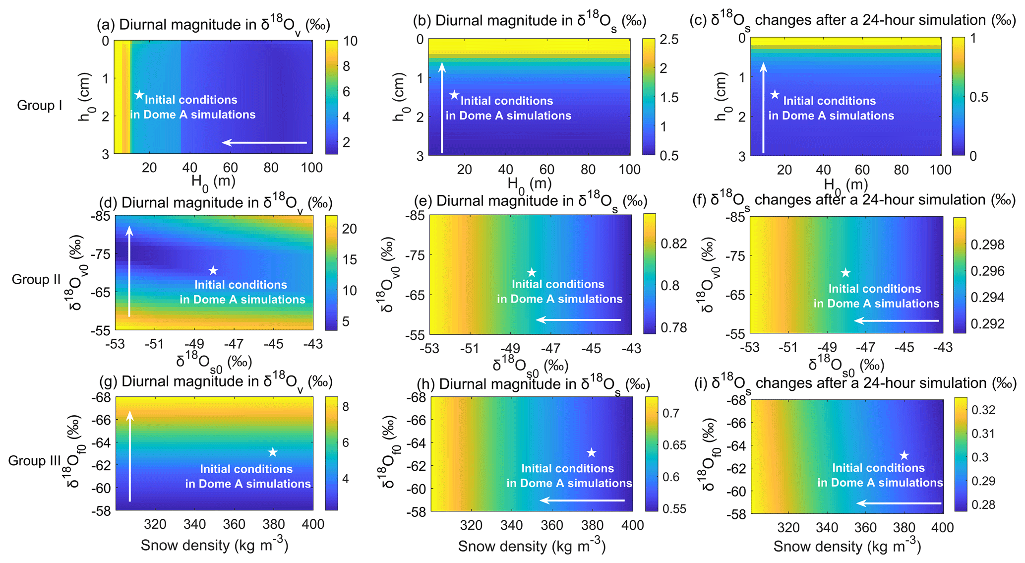
Figure 8 Sensitivity of the modeled results to changes in initial conditions. Panels (a–c) display the modeled magnitude of δ¹⁸O diurnal variations in water vapor ($\mathit{\delta }{{}^{\mathrm{18}}\mathrm{O}}_{\mathrm{v}}$), the modeled magnitude of δ¹⁸O diurnal variations in surface snow ($\mathit{\delta }{{}^{\mathrm{18}}\mathrm{O}}_{\mathrm{s}}$), and $\mathit{\delta }{{}^{\mathrm{18}}\mathrm{O}}_{\mathrm{s}}$ differences between the ending and starting values varying with different surface snow thicknesses (h₀) and boundary layer heights (H₀). Panels (d–f) show the sensitivities of the simulated results to changes in initial water vapor ($\mathit{\delta }{{}^{\mathrm{18}}\mathrm{O}}_{\text{v0}}$) and surface snow isotopic composition ($\mathit{\delta }{{}^{\mathrm{18}}\mathrm{O}}_{\text{s0}}$). Panels (g–i) are the same as (d–f) but show the sensitivities to changes in the water vapor isotopic composition of the free atmosphere ($\mathit{\delta }{{}^{\mathrm{18}}\mathrm{O}}_{\text{f0}}$) and snow density (ρ_s). In each panel, the white star indicates the initial conditions used in the Dome A simulations with summer clear-sky conditions. The white arrows correspond to the direction of the simulated results with higher sensitivity.

4 Discussion

Despite differences in the magnitudes, under summer clear-sky and highly cloudy conditions the modeled isotopes in surface snow and water vapor display clear diurnal patterns at Dome A. In both of these cases, the water vapor isotopes show a smaller magnitude of diurnal variations with respect to the snow isotopes. In general, in the period of mass exchange dominated by sublimation, snow δ¹⁸O and δD are enriched because lighter isotopes are preferentially sublimated into the atmosphere. Moreover, sublimates mixing with water vapor leads to increases in vapor δ¹⁸O and δD because they have higher δ¹⁸O and δD values than atmospheric vapor. During periods of mass exchange dominated by deposition, water vapor δ¹⁸O and δD are significantly depleted (Ritter et al., 2016). Note that the effects on snow δ¹⁸O and δD are smaller than those on vapor δ¹⁸O and δD. This is because the surface snow mass reservoir is much larger than the mass of deposition, so the associated isotope effects on surface snow are very small (Steen-Larsen et al., 2013; Casado et al., 2018).

Based on Figs. 2, 4c, 4d, 5c, and 5d, it is evident that the diurnal isotope cycles in surface snow and water vapor have a strong correlation with surface temperature and humidity. As described in Sect. 2.1, surface temperature can modify local atmospheric dynamic conditions and specific humidity, leading to synchronous responses in atmosphere–snow water vapor exchange fluxes. Temperature can also affect isotope fractionation during phase exchange. Atmosphere–snow water vapor exchange is associated with equilibrium and kinetic isotope fractionation between snow and water vapor (Ritter et al., 2016; Hughes et al., 2021; Wahl et al., 2021). The degree of isotopic equilibrium fractionation is directly dependent on the local surface temperature (Ellehoj et al., 2013), while kinetic isotope fractionation is mainly driven by the vapor pressure gradient between the snow surface and atmosphere (Jouzel and Merlivat, 1984; Surma et al., 2021; Passey and Levin, 2021). The specific humidity is also crucial because it represents the size of the water vapor reservoir with which snow can exchange (Casado et al., 2018). However, it is only important for atmospheric vapor δ¹⁸O and δD, as surface snow is a much-larger mass reservoir that buffers the effects of atmospheric vapor change. Wind speed also plays a key role in driving isotopic variations at Dome A because its increase can amplify the variations in latent heat, leading to more pronounced diurnal changes in water vapor and snow isotopic composition (Sect. S5 in the Supplement, Bréant et al., 2019).

The diurnal variations in water vapor isotopic composition resulting from the exchange between the atmosphere and snow surface are subject to influences beyond mere meteorological conditions. Specifically, fluctuations in the boundary layer height (H₀) can result in either an attenuation or an amplification of the magnitude of variations in water vapor isotopic composition (Ritter et al., 2016), as evidenced by Fig. 8a. Furthermore, the interaction between the free atmosphere and the boundary layer can significantly impact the diurnal variations in the water vapor isotopic composition (Casado et al., 2018). Specifically, during periods of intense mixing, the variations in water vapor isotopic composition become more pronounced (Fig. 8g and Sect. S4 in the Supplement). However, in the model employed for this study, the boundary layer height (H₀) and water vapor isotopic composition in the free-atmosphere layer (δf₀) are maintained as constants to simplify the calculations, whereas they vary daily in reality. This simplification for model calculations may lead to a reduction in the inter-day variability in simulated water vapor isotopic compositions (Fig. 3e).

We also compared our modeled water vapor δ¹⁸O, δD, and d-excess data at Dome A with water vapor δ¹⁸O, δD, and d-excess data from other East Antarctic interior sites from observations, such as the Kohnen station, Dome C, and a location approximately 100 km away from Dome A (Ritter et al., 2016; Casado et al., 2016; Liu et al., 2022). Both our simulations and observations have similar diurnal patterns, with high values occurring during daytime warming and low values occurring during nighttime cooling. However, it is worth noting that the magnitudes differ between the diurnal simulations at Dome A and the observations at other sites. Our modeled δD variations at Dome A (29 ‰ ± 19 ‰) are lower than the observed diurnal variations in water vapor δD at Kohnen station (36 ‰ ± 6 ‰ from Ritter et al., 2016) and at Dome C (38 ‰ ± 2 ‰ from Casado et al., 2016). This difference can be attributed to the atmospheric dynamic conditions at Dome A, which are characterized by a lower daily mean wind speed (2.8 m s⁻¹) than that at Dome C (3.3 m s⁻¹) and Kohnen station (4.5 m s⁻¹) during the summer season (Casado et al., 2018). A lower wind speed corresponds to relatively weak air convection in the vertical direction. Due to the coupling between upper- and lower-atmospheric layers, vertical turbulent mixing may decrease with weakened air convection in the atmospheric near-surface layer (Casado et al., 2018). This change can attenuate molecular exchange between surface snow and water vapor, leading to a muted fluctuation in the modeled water vapor δD in combination with less mass exchange. In addition, the simulated diurnal changes in water vapor isotopic composition are lower than those observed at sites near Dome A (>40 ‰ for δ¹⁸O and 200 ‰ for d-excess). This large discrepancy may be due to calibration drifts caused by the low-water-vapor content during the measurements at the nearest Dome A site (Liu et al., 2022).

The magnitudes of the modeled diurnal changes in snow δ¹⁸O and δD are different between highly cloudy and clear-sky conditions, with apparently small magnitudes under cloudy conditions. It seems that when clouds are present, surface snow will receive longwave radiation from clouds and be less influenced by solar radiation. As a result, the diurnal radiation budget cycle is less variable than that on days without clouds, as otherwise, solar radiation with a strong diurnal cycle becomes the most significant variable. On days with clouds, the diurnal variations in air temperature and surface temperature are also smaller, and the differences between the air temperature and surface temperature during the day and night become less pronounced (Fig. 2). This could have a negative impact on the changes in atmospheric dynamics between day and night. The diurnal variations in the wind speed and friction velocity are thus not significant (Figs. 2, 4b, and 5b). The vertical turbulent mixing between surface snow and water vapor in a diurnal cycle is relatively stable. This results in reduced mass exchange and a decrease in the isotope effects occurring between these two reservoirs.

The model results for summer clear-sky and highly cloudy conditions also indicate that after a 24 h simulation, δ¹⁸O and δD in surface snow are enriched mainly due to isotope fractionation during sublimation. Notably, although water vapor with much-lighter δ¹⁸O and δD values than snow are deposited in the deposition period, the masses are negligible compared to those in the snow mass reservoir, so the effects on snow isotopes in the 24 h simulation period are dominated by the effects of sublimation. The enrichments in snow isotopes caused by sublimation are consistent with previous studies (e.g., Ritter et al., 2016; Casado et al., 2018; Hughes et al., 2021). In addition, sublimation is associated with snow mass loss. Many studies also indicate significant surface snow mass loss during summer due to sublimation at inland Antarctic sites including Dome A (e.g., Frezzotti et al., 2004; Ding et al., 2016). As such, at Dome A, surface snow isotopes are presumably enriched during summer. Using a simple Rayleigh distillation model, Pang et al. (2019) predicted that over summer ∼2 ‰ enrichments in surface snow δ¹⁸O can be caused under mean Dome A summer conditions.

Based on the results of the sensitivity tests, diurnal variations in isotopic composition of snow due to water vapor exchange processes can also be influenced by several parameters, such as snow thickness, snowfall isotopic composition, snowfall density, and surface roughness (refer to Fig. 8 and Sect. S5). Among these factors, changes in snowpack thickness exhibit the most pronounced impact on the isotopic effects of water vapor exchange processes. Specifically, when the snow thickness exceeds 3 cm, the water vapor exchange effect struggles to induce inter-day variations in snow isotopes. On the other hand, the effects of snowfall isotopic composition, snowfall density, and surface roughness on the isotopic composition of surface snow may be limited during the Dome A summer season (Sect. S5), given the realistic range of potential variations in snowpack parameters.

Under the typical winter conditions at Dome A, temperature and humidity remain relatively constant throughout the day (i.e., during a 24 h simulation period). The Richardson number (Ri) is positive throughout the day, indicating stable atmospheric conditions. As a result, the diurnal variations in the exchange of atmospheric water vapor and snow isotopes are less pronounced. Specifically, the model simulations suggest that under these conditions only deposition occurs, leading to a depletion of snow isotopes (δ¹⁸O and δD) after the 24 h simulation period.

Because the diurnal variations in snow isotopic composition induced by atmosphere–snow water vapor exchange in summer and winter are different, seasonal snow isotopic changes can be affected. In particular, according to the modeled results, in summer surface snow δ¹⁸O and δD should become more enriched than fresh snow, while in winter surface snow isotopes should be less abundant than in fresh snow. This effect appears to be distinct from what can be expected from other post-depositional processes. For example, Town et al. (2008) demonstrated that wind-driven ventilation after snowfall can result in isotope enrichment in winter snow layers and depletion in summer snow layers, decreasing the magnitude of seasonal variations. Vapor diffusion in snow pores also contributes to the attenuation of δ¹⁸O or δD seasonal variations by smoothing (Johnsen et al., 2000; Casado et al., 2020). To evaluate the annual net effect of atmosphere–snow water vapor exchange, the potential mass loss in summer and gain in winter must be estimated. From just the continuous simulations of this study, it appears that the annual net effects should lead to isotopic enrichment in the snow layer since the magnitudes of isotopic changes in summer are much larger than those in winter. However, we note that the continuous simulation in this study was conducted without differentiating between clear-sky and cloudy conditions and was considerably affected by the abrupt temperature fluctuations observed at Dome A. Therefore, further exploration of continuous simulations is required, which can be achieved through improvements in model refinement and the capabilities of observational techniques with more-precise data available.

5 Conclusions

Atmosphere–snow water vapor exchange is important for snow isotope preservation as suggested by previous studies (Ritter et al., 2016; Hughes et al., 2021; Hu et al., 2022). In this study, we constructed a new box model based on the bulk aerodynamic method to predict changes in surface snow and water vapor isotopic compositions in response to diurnal fluctuations in local meteorological conditions. The model was validated by the agreement between the modeled and observed diurnal cycles of water vapor δ¹⁸O, δD, and d-excess at Dome C and then applied to investigate the degree of atmosphere–snow water vapor exchange and the associated isotope effects at Dome A at diurnal scales. The model results show that atmosphere–snow water vapor exchange at Dome A can also lead to similar diurnal isotope variations in atmospheric water vapor δ¹⁸O and δD under summer conditions, with corresponding diurnal variations in surface snow δ¹⁸O and δD. For clear-sky conditions, the magnitudes of the diurnal cycles in snow and water vapor isotopes are greater than those in simulations under highly cloudy conditions. In addition, we performed diurnal simulations under Dome A winter conditions. The results indicate that the diurnal isotope variations over the 24 h simulation period are less significant due to the stable atmospheric conditions with low and relatively stable air temperature and specific humidity. However, the model results suggest that snow isotope depletion can occur in winter. The modeled opposite isotope effects on snow after 24 h in winter and summer at Dome A suggest that atmosphere–snow water vapor exchange could increase the seasonal snow isotope variations. The modeled changes in winter are smaller than those in summer due to the highly stable boundary layer conditions in winter. This means that the effects in summer cannot be offset by those in winter, leading to overall enrichments of snow isotopes.

We also acknowledge the limitations inherent to our simulations with a one-dimensional model. The air mass exchange process between the free-atmosphere layer and boundary layer may play an important role in atmosphere–snow water vapor exchange as observed during some frost events (Casado et al., 2018). Although the influence of the free atmosphere has been incorporated into our model, it is worth refining the underlying assumptions for the air mass exchange process and improving the accuracy of the model simulations. Further, observational validation of the model results for the winter season is unavailable due to extremely harsh conditions at Dome A. Although it is currently difficult to conduct fieldwork at the diurnal scale there, observations at longer timescales (e.g., weekly resolved sampling of surface snow and precipitation over a year along with a snowpack to reconstruct the changes after deposition) could be possible. These results are important to validate the model's ability to predict the associated isotope effects of atmosphere–snow water vapor exchange, especially considering that the model implies that atmosphere–snow water vapor exchange may have few isotope effects at the annual scale but tends to increase snow water isotope seasonality. The latter is opposite to other post-depositional processes such as wind-driven ventilation (Town et al., 2008) and vapor diffusion in snow pores (Johnsen et al., 2000).