The influence of present-day regional surface mass balance uncertainties on the future evolution of the Antarctic Ice Sheet

Rising global sea levels are one of many impacts associated with current anthropogenic global warming. The Antarctic Ice Sheet (AIS) has the potential to contribute several meters of sea level rise over the next few centuries. To predict future sea level rise contributions from ice sheets, both global and regional climate model (RCM) outputs are used as forcing in ice sheet model simulations. While the impact of different global models on future projections is well-studied, the effect of different regional models on the evolution of the AIS is mostly unknown. In our study, we present the impact of the choice of present-day reference RCM forcing on the evolution of the AIS. We used the Parallel Ice Sheet Model (PISM) to study the AIS in a quasi-equilibrium state and under future projections, combining present-day RCM output with global climate model projections. Our study suggests differences in projected Antarctic sea level contributions due to the choice of different present-day surface mass balance (SMB) and temperature baseline forcings of 10.6 mm in the year 2100 and 70.0 mm in 2300 under the RCP8.5 scenario. Those uncertainties are an order of magnitude smaller than what is estimated from uncertainties related to ice sheet and climate models. However, we observe an increase in RCM-induced uncertainties over time and for higher-emission scenarios. Additionally, our study shows that the complex relationship between the selected RCM baseline climatology and its impact on future sea level rise is closely related to the stability of West Antarctic Ice Sheet (WAIS), particularly the dynamic response of Thwaites and Pine Island glaciers. On millennial timescale, the choice of the RCM reference leads to ice volume differences up to 2.3 m and can result in the long-term collapse of the West Antarctic Ice Sheet.

1 Introduction

Global sea level rise is one of many climate impacts due to anthropogenic global warming (IPCC, 2022). Until the end of this century, model-based estimates of global sea level rise range from 0.44–0.76 m for SSP3-4.5 (IPCC, 2022) threatening flood-prone areas populated by over 420 million people (Hooijer and Vernimmen, 2021). Besides ocean thermal expansion, the melting of the Greenland and Antarctic ice sheets is the largest current contributor to sea level rise (IPCC, 2022). Despite the fact that the Antarctic Ice Sheet (AIS) is 7.8 times larger than the Greenland ice sheet (GrIS) (Morlighem et al., 2017, 2020), it currently contributes 3.6 ± 0.5 mm per decade to global sea level rise (Rignot et al., 2019), which is an almost 2 times smaller contribution compared to the GrIS (WCRP Global Sea Level Budget Group, 2018). However, observations show that the Antarctic melt contribution has been accelerating (Otosaka et al., 2023) and could become the largest contributor by the end of the century (Seroussi et al., 2020). The marine parts of the West Antarctic Ice Sheet (WAIS), which holds ice masses equivalent to ca. 3.3 m of sea level rise (Bamber et al., 2009), might undergo a rapid melt in the coming centuries due to its exposition to the so-called marine ice sheet (MISI Schoof, 2007; Pattyn, 2018) and ice cliff instabilities (MICI DeConto and Pollard, 2016; Pattyn, 2018). Model-based projections of Antarctic sea level contributions at the end of the century are associated with large uncertainties, which can be reduced by careful calibration of the model (Bevan et al., 2023; Nias et al., 2019; Coulon et al., 2024; Edwards et al., 2019; Lowry et al., 2021). Ice sheet model projections of sea level equivalent ice volume change vary from −37 ± 34 to 96 ± 76 mm by the year 2100 (Seroussi et al., 2020) for the RCP8.5 scenario. This uncertainty has many reasons, spanning from largely unconstrained boundary conditions like basal friction (Bulthuis et al., 2019), ice shelf mass balance uncertainties arising from melt rate parameterizations and projected ocean temperature changes below the ice shelves, and the evolution of the surface mass balance (SMB) (Coulon et al., 2024). Uncertainties in estimates of Antarctica's SMB – the net accumulation rate of snow and ice on the surface of Antarctica – have been discussed in detail recently (Mottram et al., 2021). Direct observations of accumulation and surface melt are sparse, while SMB products from regional climate models have a large spread ranging from 1961 ± 50 to 2519 ± 118 Gt yr⁻¹ (Mottram et al., 2021).

Uncertainties in Antarctica's current SMB affect prognostic or paleo ice sheet model (ISM) simulations, which often use output from regional climate models (RCMs) as a reference baseline forcing upon which climate anomalies are then added. The SMB data from RCMs are used to establish the present-day reference forcing, and projections or reconstructions of future and past Antarctic climate change are added to this forcing via anomalies, usually computed against the pre-industrial or historical mean of the respective climate model (Sutter et al., 2019; Nowicki et al., 2020; Seroussi et al., 2020; Sutter et al., 2021; Reese et al., 2023). There is a variety of different RCM SMB products available for ice sheet modeling, from which a selection is presented in Fig. 1. Those SMB fields not only differ in the total SMB they produce for Antarctica but also in the spatial distribution (Mottram et al., 2021). However, many modeling studies utilize data from the RACMO model (Seroussi et al., 2020). This model is designed to simulate polar regions since it accounts for many relevant processes, such as snow drifting, melt, refreezing and percolation (van Wessem et al., 2018). However, there is not a specific reason to exclusively use one model, since other models are also designed to simulate polar regions by taking those processes into account (Mottram et al., 2021). A recent study by Li et al. (2023) suggests that the difference in SMB from different global models can have a substantial impact on the equilibrium state of the AIS. Furthermore, Seroussi et al. (2020) showed that there is also a significant impact of global climate model (GCM) differences in future projections.

In this study we investigate the response of the AIS to different forcings derived from a range of RCMs. We address the following questions. (i) How does the choice of reference SMB and surface air temperature forcing affect the quasi-equilibrium state of the AIS? (ii) How does this choice affect the evolution of the AIS under different climate scenarios? (iii) Does this choice have an impact on the projected stability of marine ice sheets?

In the following sections, we introduce the RCM products utilized in our study and describe our simulation setup for the AIS. We then present the results from our long-term equilibrium simulations and future projections. Finally, we discuss the implications of the choice of RCM product on the evolution and stability of the AIS.

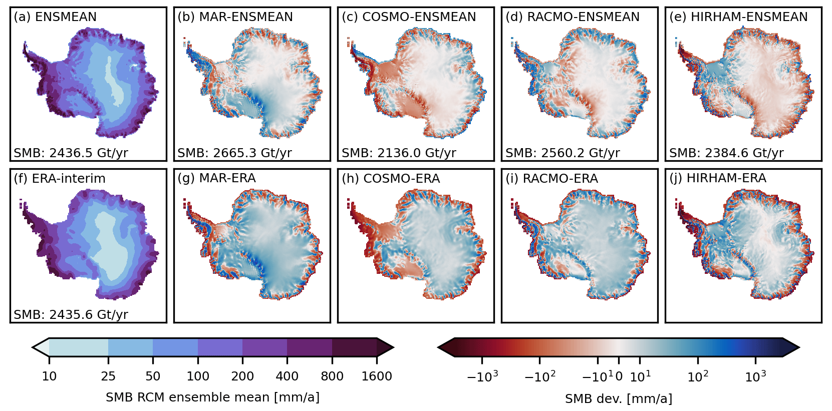
Figure 1 Surface mass balance (SMB) of the (a) multi-RCM mean and anomalies of the (b) MARv3.10 (Kittel et al., 2020), (c) COSMO-CLM² (Souverijns et al., 2019), (d) RACMO2.3p3 (van Dalum et al., 2022), and (e) HIRHAM5 (Hansen et al., 2022) regional climate model from this mean. SMB of the ERA-Interim dataset (Dee et al., 2011) (f). SMB differences between (g) MARv3.10, (h) COSMO-CLM², (i) RACMO2.3p3, (j) HIRHAM5 and ERA-interim. The surface mass balance was averaged over the period from 1987–2016.

2 Methods

To address the questions posed above, we consider two different model setups. In the first, we assess the equilibrium ice sheet response for a range of reference present-day baseline climate forcings. In the second, we investigate the imprint of the present-day baseline climatology on ice sheet model projections under a set of CMIP5 scenarios. In the following we will briefly describe the ice sheet model setup (spinup, present-day equilibrium and prognostic simulations) and introduce the applied regional climate model forcing which will be used as a baseline climatology in all experiments.

2.1 SMB forcings

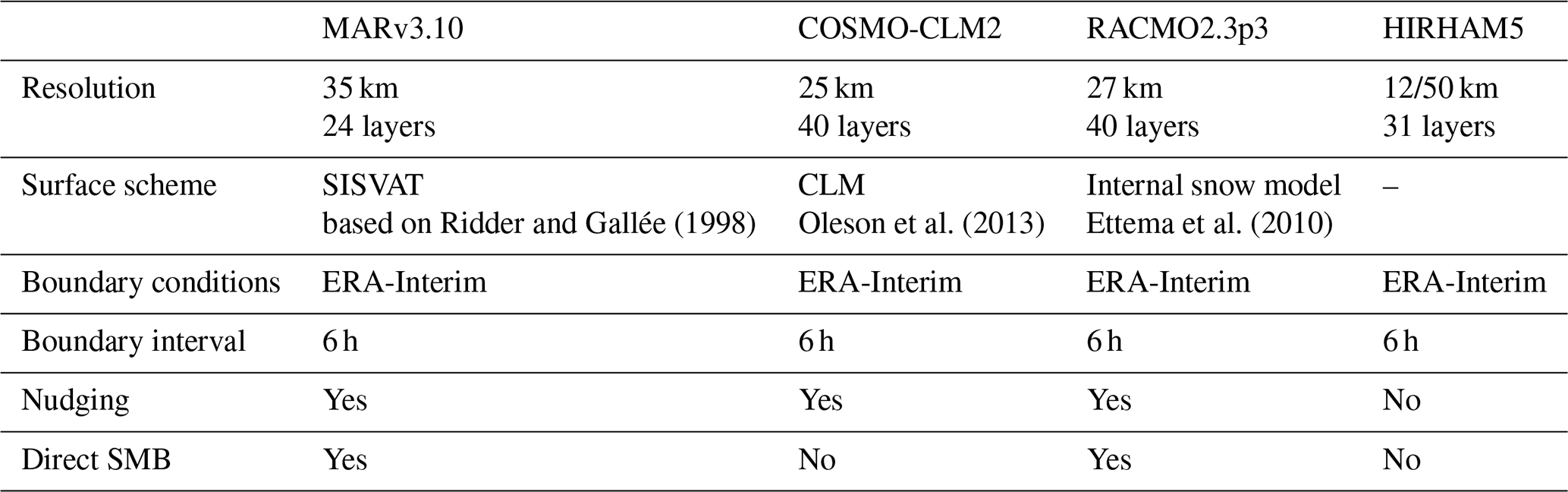
There is a considerable spread of model-based present-day surface mass balance (SMB) estimates (Mottram et al., 2021) (see Fig. 1). To assess the equilibrium and transient ice sheet response to this spread we force the ISM with surface air temperature and surface mass balance derived from four regional climate models (RCMs): MARv3.10 (Mottram et al., 2021; Kittel et al., 2020), COSMO-CLM² (Souverijns et al., 2019), RACMO2.3p3 (van Dalum et al., 2022, 2021) and HIRHAM5 (Hansen et al., 2022, 2021b). A general overview of these models and the applied forcings, parameterizations and submodules is provided in Table 1. An additional SMB comparison for the individual Ice sheet Mass Balance Inter-comparison Exercise (IMBIE) drainage basins can be found in Fig. A1. All four models were forced with the ERA-Interim reanalysis (Dee et al., 2011) at the domain boundaries, with the MARv3.10, RACMO2.3p3 and COSMO-CLM² model being nudged into the domain by applying upper air relaxation (van de Berg and Medley, 2016). In contrast HIRHAM evolved freely and was only forced at the boundary of the domain (Mottram et al., 2021). RACMO and MAR have optimized subsurface snow and ice schemes to take meltwater, refreezing and retention into account. Additionally, RACMO accounts for wind-driven erosion and sublimation of blown-off snow (Lenaerts et al., 2012). A more detailed discussion and comparison of the applied RCMs can be found in Mottram et al. (2021). Please note that Mottram et al. (2021) used data from RACMO2.3p2, while this study uses RACMO2.3p3.

To conduct our study, we obtained the SMB forcing either directly from the model output (MAR and RACMO) or calculated SMB as described by Mottram et al. (2021) from precipitation, evaporation and sublimation. Please note that for COSMO the difference between precipitation and evaporation is used to calculate the SMB, and for HIRHAM the difference between precipitation, sublimation, and evaporation is used for the same purpose. We then calculated the climatic mean of the SMB and surface temperature for the common period from 1987 to 2016 and bi-linearly regridded the data to the ISM domain at 8 km resolution. The SMB ensemble mean of those RCMs, the deviation of the individual RCM SMBs from this mean and the total mass balance are shown in Fig. 1. Please note that due to the regridding and the chosen ice mask we expect the total SMB to differ slightly from values of other publications (Hansen et al., 2022).

Ridder and Gallée (1998)Oleson et al. (2013)Ettema et al. (2010)

Table 1 Summary of the regional climate model configuration for MARv3.10 (Kittel et al., 2020), COSMO-CLM2 (Souverijns et al., 2019), RACMO2.3p3 (van Dalum et al., 2022) and HIRHAM5 (Hansen et al., 2021a).

2.2 Ice sheet model setup

To simulate the response of the Antarctic Ice Sheet, we employ the thermodynamically coupled Parallel Ice Sheet Model (PISM) (Bueler and Brown, 2009; Winkelmann et al., 2011). PISM is used in a hybrid mode using the shallow ice (SIA) and shallow shelf approximation (SSA) to efficiently simulate the slow interior ice sheets and the fast ice streams of outlet glaciers and shelves. The stress at which the ice starts to slide by deformation of the till layer, also called yield stress is calculated following the Mohr–Coulomb law (Cuffey and Paterson, 2010),

$$\begin{array}{}\text{(1)}& {\mathit{\tau }}_{\mathrm{c}}=c_{\mathrm{0}}+\tan \left(\mathit{\varphi }\right)N_{\mathrm{till}},\end{array}$$

with the till friction angle ϕ, the effective till pressure N_till and the “till cohesion” c₀. The till friction angle depends on the bed topography and is linearly interpolated between ϕ_min and ϕ_max for bed elevations between b_min and b_max with the gradient $M=({\mathit{\varphi }}_{\max }-{\mathit{\varphi }}_{\min })/(b_{\max }-b_{\min })$ by

$$\begin{array}{}\text{(2)}& \begin{array}{rl}& \mathit{\varphi }(x,y)=\\ & \left\{\begin{array}{ll}{\mathit{\varphi }}_{\min },& b(x,y)\le b_{\min },\\ {\mathit{\varphi }}_{\min }+\left(b\right(x,y)-b_{\min })M,& b_{\min }<b(x,y)<b_{\max },\\ {\mathit{\varphi }}_{\max },& b_{\max }\le b(x,y)\end{array}\right.\end{array}\end{array}$$

(Aschwanden et al., 2013; Winkelmann et al., 2011; Martin et al., 2011). Sub-shelf melt and refreezing at the ice–ocean interface is calculated using PICO (Reese et al., 2018), an ocean box model that mimics the overturning circulation in the cavities below the ice shelf.

In this study we consider two model setups (see Fig. 2): (i) A long-term (30 kyr) present-day equilibrium simulations with a constant present-day forcing and (ii) centennial projections until the year 2300 applying climate anomalies from HadGEM-ES2 (Jones et al., 2018) for the RCP2.6, RCP4.5 and RCP8.5 scenarios. In both cases, the model is initialized from the BedMachine (Morlighem et al., 2020) bedrock topography and ice thickness. Additionally, geothermal heat flux data from Shapiro and Ritzwoller (2004) are applied.

2.2.1 Long-term present-day equilibrium simulations

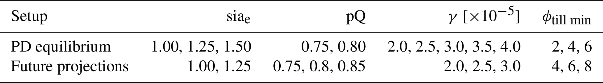
To explore the equilibrium response of the Antarctic Ice Sheet to the four RCM forcings considered here, we perform a set of long-term present-day equilibrium simulations. As an initial step we perform a 200 kyr thermal spinup during which the ice surface elevation is fixed and the ice sheet is forced with geothermal heat flux from Shapiro and Ritzwoller (2004) and surface air temperature from MARv3.10 (Kittel et al., 2020), COSMO-CLM2 (Souverijns et al., 2019), RACMO2.3p3 (van Dalum et al., 2022) and HIRHAM5 (Hansen et al., 2021a) (see Fig. 2). After the thermal spinup, we restart the ice sheet model from the thermal spinup for each RCM individually. We apply constant SMB and temperature forcing fields from the individual RCMs and let the model freely evolve for 30 000 years (see Fig. 2) at a 16 km resolution. A summary of the described simulation setups can be found in Table B2. To compute basal melting underneath the ice shelves, we additionally force the model with ocean temperature and salinity from the observational climatology provided in the ISMIP6 protocol (Nowicki et al., 2020). For every RCM forcing, we run 24 simulations with different combinations of the shallow ice approximation enhancement factor sia_e, the pseudo-plastic parameter pQ (used in the pseudo-plastic sliding law), the minimum till friction angle ϕ_min (the angle we assume for marine basins below −700 m as in Albrecht et al., 2020b) and the heat conductivity at the ice–ocean interface γ. For a detailed list of the parameters, see Tables 2 and B1. The parameter combinations were selected based on the model skill to reproduce the observed present-day ice thickness, surface velocities and grounding line (Morlighem et al., 2020) after 15 000 years under constant RACMO forcing. An additional constraint was the sea level equivalent ice volume after 15 000 years under constant RACMO2.3p3 forcing. Here we penalized deviations from present-day estimates of Antarctica's current ice volume. The comparison and scoring was performed following the scoring method by Albrecht et al. (2020b). The chosen spinup method and parameter selection process is not necessarily the most rigid in terms of producing a good match with present-day ice sheet observations. A much better fit can be achieved, for example, via inversion or iterative optimization of a sliding parameter as done in Pollard and DeConto (2012) and Li et al. (2023). The latter method can either be applied for only one forcing or for all forcings individually. Nevertheless, both approaches have drawbacks when applied to our context. On the one hand, individually applying the inversion or iterative optimization technique to each forcing field would select basal sliding properties for each forcing field in a manner that converges toward a state closest to observational data, thereby concealing disparities inherent to the forcing fields within the basal sliding coefficient and parameterization. This evidently runs counter to the core objective of this study, which centers around discerning the distinct influences exerted by individual forcing fields on the ice sheet.

Conversely, fine-tuning the basal sliding coefficients exclusively to a specific forcing field carries the risk of overly tailoring the model to that particular forcing field, potentially leading to overfitting. Such meticulously calibrated basal sliding conditions might not be suitable for other forcing fields, potentially resulting in unrealistic ice sheet dynamics when subjected to those fields. Generally, this trade-off necessitates consideration for each instance of tuning and parameter selection. Nonetheless, our approach employs consistent basal sliding conditions across all forcing fields, while also calibrating for overarching global parameters. This not only reduces the computational cost but also mitigates the possibility of introducing artifacts by excessively tuning the model to any single forcing field.

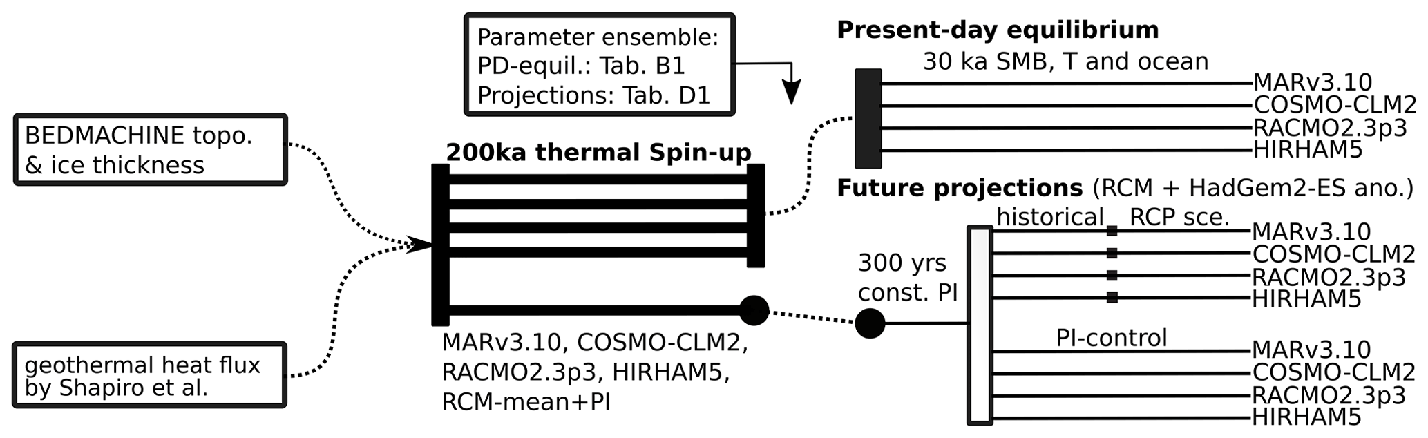
Figure 2 Illustration of the present-day equilibrium simulation and future projections setup. Starting from present-day ice sheet geometry, a 200 kyr thermal spinup for each RCM forcing is performed individually (indicated by solid bold lines). During the thermal spinup, the ice sheet geometry is fixed. For the present-day equilibrium, 24 individual simulations (see Table B1) are performed for each of the four constant RCM forcing fields while allowing the model to freely evolve for 30 000 years. Freely evolving ensemble simulations are indicated by solid thin lines. For illustrative reasons the same start and end states are connected by dashed lines. For the future projections, a 200 kyr thermal spinup under the mean forcing of all four RCMs together with HadGem2-ES (Jones et al., 2018) pre-industrial–present-day (PI–PD) anomalies is performed. Starting after the thermal spinup, a 300-year relaxation for 12 individual parameter configurations (see Table C1), using constant PI forcing, is performed. Following this, we simulate the historical period followed by the three RCP scenarios for every combination of the RCM forcing fields. All simulation setups are summarized in Table B2.

2.2.2 Centennial projections of Antarctic Ice Sheet evolution

In order to assess the impact of present-day baseline climate forcings on centennial sea level projections we perform simulations until the year 2300 applying transient annual climate anomalies derived from HadGem2-ES (Jones et al., 2018) RCP scenarios. Starting from the BedMachine (Morlighem et al., 2020) bedrock topography and ice thickness, we perform a 200 kyr thermal spinup under a constant pre-industrial (PI) temperature forcing. The pre-industrial temperature forcing is the mean of all four RCMs together with HadGem2-ES (Jones et al., 2018) pre-industrial to present-day (PI–PD) anomalies. After the thermal spinup we restart the model on 8 km resolution for 12 different parameter configuration (see Tables 2 and C1) to evolve under constant RCM mean PI forcing for 300 years to relax the initial shock after the ice can flow freely, which leads to 12 initial pre-industrial ice sheet geometries, one for each parameter configuration. At the end of the 300-year relaxation each simulation has an annual sea level contribution of below 0.15 mm yr⁻¹ and a grounding line close to present-day observation. From these initial geometries, we then branch off four 440-year PI-control simulations, one for each RCM baseline. Additionally, we simulate the historical period from 1860–2005 CE (see Fig. 2) for each RCM baseline. For the historical period and future projections, transient annual mean surface air temperature and SMB anomalies from HadGEM2-ES (Jones et al., 2018) are added to the respective present-day RCM climatology to produce the climate forcing until the year 2300. Likewise, ocean temperature and salinity anomalies are added to the ISMIP6 ocean forcing. After the historical period we branch the individual simulations into three different forcing scenarios and let the model evolve until the year 2300. The three different branches consist of the RCP2.6, RCP4.5 and RCP8.5 scenarios that use the anomalies from the HadGEM2-ES model. Similar to the present-day equilibrium runs, we choose an ensemble of different parameter configurations. The complete list of selected parameter configurations is provided in Tables 2 and C1. Please note that since the model spinup (thermal + constant PI forcing) we chose here is relatively simple compared to, e.g., inversion or a full glacial interglacial paleo-spinup, remaining model biases are to be expected. As a consequence, the initial ice sheet configuration lacks a realistic thermal state. In addition, as we do not use iterative optimization (see above), model deviations with respect to ice thickness between a simulated present-day state and observations can be large, which is typical of continental-scale model setups not employing inversion methods (e.g., Reese et al., 2023). However, as these kinds of simple spinup (thermal + constant PI forcing) routines have been used in the past (Seroussi et al., 2019; Levermann et al., 2020; Sutter et al., 2023), we considered this to be a valid approach to assess the impact of present-day climate forcing uncertainties on future and equilibrium ice sheet evolution in typical model setups. Therefore, this setup is not designed to give robust projections on future Antarctic sea level contributions but rather serves to estimate uncertainties arising from different RCM forcing fields.

Table 2 Chosen parameter space for the shallow ice approximation enhancement factor sia_e, the pseudo-plastic pQ factor, the heat conductivity at the ice–ocean interface γ, and the minimum till friction angle ϕ_{till min} for the present-day equilibrium runs and future projections. A detailed list of every individual parameter configuration can be found in Tables B1 and C1.

3 Results

In this section we present the evolution of ice volume and area under constant present-day forcing and centennial future projections. We further discuss the imprint of SMB forcing differences on ice thickness and grounding line position at the end of the respective simulations.

3.1 Impact of RCM forcing on the present-day quasi-equilibrium state

3.1.1 Impact of RCM forcing on global ice mass and extent

Starting from the present-day observations, the total ice volume (see Fig. 3a–d) undergoes an initial shock after which the rate of change (see Fig. 3e–h) converges towards zero. After 30 000 years of simulation the median change in ice volume is negative (i.e., ice loss) for three (COSMO: −1.71 m; RACMO: −1.20 m; HIRHAM: −1.63 m) out of the four models. The simulations that apply the RACMO forcing show the least change in ice volume. In contrast, ice sheet simulations using the MAR forcing exhibit an increase in median sea level equivalent (SLE) ice volume compared to present-day observations by 0.55 m. Although the annual rate of mass change converges towards zero, the ensemble spread indicates that the ice sheets are still undergoing small fluctuations in ice sheet mass between −0.20 and 0.10 mm yr⁻¹ (current AIS sea level contribution is ≈0.3 mm yr⁻¹; Shepherd et al., 2018). The initial shock observed in the ice volume change is also reflected in the respective ice area change in floating and grounded ice. For all models an increase in the grounded ice area with a coinciding decrease in the ice shelf area is observable – a result of an advancing grounding line in the Filchner–Ronne Ice Shelf (see Fig. 4). The median decrease in ice shelf area varies between −43 % and −36 %, with COSMO and MAR showing the largest and smallest decrease, respectively. This might be due to a stronger grounding line retreat, especially when WAIS is unstable, allowing for larger shelves. Additionally, we observe a grounding line advance with MAR showing the largest (3.4 %) and COSMO the smallest (2.8 %) corresponding growth in grounded ice area. The time series presenting the impact of the ensemble mean RCM forcing can be found in Fig. B3.

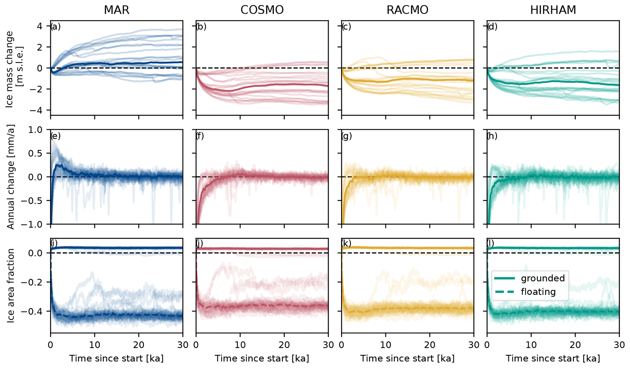
Figure 3 Time series of the total ice mass above flotation change since the start of the simulation (a–d), the annual rate of ice mass above flotation change (e–h), and the fraction of grounded (solid line) and floating (dashed line) ice area (i–l) relative to observations for the four different RCM forcing fields. The bold line shows ensemble median, while the shaded lines indicate the individual ensemble members.

3.1.2 Impact of RCM forcing on regional ice cover

We now turn to regional characteristics of the simulated ice sheet. When we compare the ice thickness between present-day observations and our simulations after 30 000 years a distinct pattern arises that is independent of ensemble member and RCM forcing field (see Fig. B1). All of our simulations show a strong negative ice thickness anomaly in the WAIS that is mainly driven by ice sheet model parameterization. Specifically, the applied heuristics calculating the till friction angle result in anomalies with respect to present-day observations. This is a persistent model bias for the setup employed here and in other studies (Martin et al., 2011; Albrecht et al., 2020a; Sutter et al., 2023; Reese et al., 2023). Additionally, all realizations show ice loss at the East Antarctic Ice Sheet (EAIS) margins with substantial coastal ice sheet thinning in George V Land and Wilkes Land. In contrast, larger ice thickness is simulated in Oates Land along the Transantarctic Mountains, on the Antarctic Peninsula, in the Ellsworth and Scott mountains, and in the Shackleton Range. The inter-model differences caused by the different RCM forcings (mainly the impact of SMB forcing differences) are around 4 times smaller than the overall model bias (effect of ice sheet model spinup and parameter choices mentioned above).

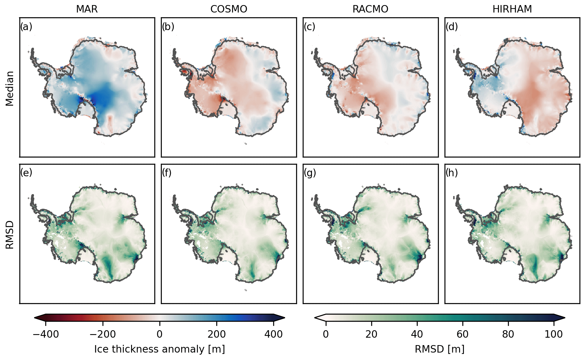
Figure 4 (a–d) Ice thickness anomalies Δh from the common mean position of the simulated (grey) grounding line for the present-day equilibrium simulations. (e–h) Root-mean-square deviation (RMSD) of the individual ensemble members from the median. The difference between the common mean and the result of the forcing ensemble mean are illustrated in Fig. B4.

Therefore, we explicitly illustrate the differences between the individual RCM forcing sets in Fig. 4. Figure 4a–d depict the ice thickness differences Δh for each individual RCM forcing set from the common mean of all four forcing sets. At every grid cell (i,j) and for a given $\mathrm{RCM}\in \mathit{\{}\mathrm{MAR},\mathrm{COSMO},\mathrm{RACMO},\mathrm{HIRHAM}\mathit{\}}$, Δh is given as follows:

$$\begin{array}{}\text{(3)}& \mathrm{\Delta }{h}_{i,j}^{\mathrm{RCM}}=h_{i,j}^{\mathrm{RCM}}-{\displaystyle \frac{h_{i,j}^{\mathrm{MAR}}+h_{i,j}^{\mathrm{COSMO}}+h_{i,j}^{\mathrm{RACMO}}+h_{i,j}^{\mathrm{HIRHAM}}}{\mathrm{4}}}.\end{array}$$

Due to its overall higher SMB, the simulations forced with the MAR data show positive Δh, except for small negative Δh values at the Princess Ragnhild Coast and George V Land. Additionally, simulations forced with SMB and surface temperature from COSMO, RACMO and HIRHAM show diverging Δh patterns between East and West Antarctica that generally agree with the differences in their underlying SMB forcing. For all four forcing fields we illustrate the regions of highest ensemble variability in ice thickness (Fig. 4e–f). We do this by calculating the root-mean-square deviation (RMSD) of Δh from the parameter ensemble mean for each RCM. The Wilkes and Aurora subglacial basins are the regions of highest ensemble variability. Additionally, the Shackleton Range shows large ice thickness variability across all four forcing fields. The HIRHAM forcing field exhibits high variability in Ellsworth Land.

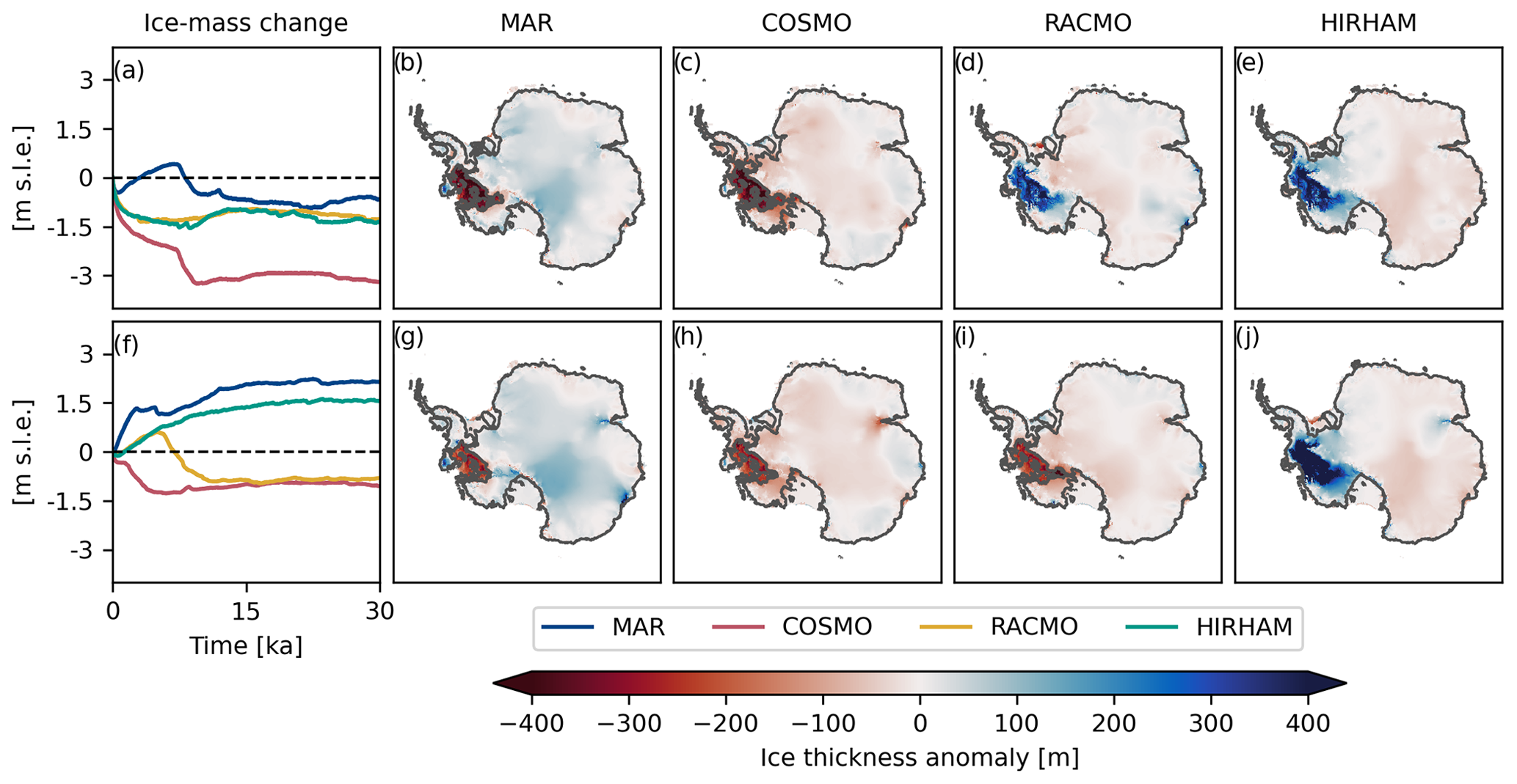
Figure 5 Evolution of the ice masses relevant to sea level change (a, f) over the simulation period and ice thickness differences from the common mean and grounding line position (grey line) at the end of the simulation (b–e, g–j). Panels (a)–(e) show the results of the simulation with ϕ_min=2°, sia_e=1.00, pQ =0.8, and $\mathit{\gamma }=\mathrm{4.0}\times {\mathrm{10}}^{-\mathrm{5}}$. Panels (f)–(j) show the results the simulation with ϕ_min=6°, sia_e=1.50, pQ =0.80, and $\mathit{\gamma }=\mathrm{2.5}\times {\mathrm{10}}^{-\mathrm{5}}$.

3.1.3 Amplification of ISM uncertainties due to RCM selection

In order to illustrate differences in individual model runs and their evolution under constant present-day climate conditions, we illustrate the change in ice volume and ice thickness differences at the end of the simulation (after 30 kyr) for parameter configuration nos. 6 and 24 (see Table B1) in Fig. 5.

Under parameter configuration no. 6 (Fig. 5a–e), the simulations forced by RACMO and HIRHAM undergo initial ice loss until they mostly stabilize for the rest of the simulation period. In contrast, the simulations forced by COSMO and MAR show an initial ice mass increase (MAR) or decrease (COSMO) for the first 7000 years. Both simulations then exhibit a dynamical reorganization of WAIS, leading to a strong grounding line retreat and ice mass loss of over 1 m s.l.e. While in the COSMO-forced simulation the retreat of the grounding line slowly begins from the start of the simulation for several thousand years leading to the fast collapse of WAIS (see Fig. B5), the MAR simulation exhibits no differences in grounding line position from the HIRHAM- or RACMO-forced simulations for the first 6000 years (see Fig. B5). Similar behavior can be observed for parameter configuration no. 24 (Fig. 5j–f), where the relatively small differences in SMB forcing lead to large differences in the simulation outcome. In this case, all but the simulation forced by HIRHAM exhibit a dynamical collapse of WAIS.

3.2 Projections of present-day RCM imprint on centennial Antarctic Ice Sheet evolution

To investigate the effect of differences in the underlying RCM baseline data in climate scenarios, we simulated the historical period from 1860 to 2005, followed by the RCP2.6, RCP4.5 and RCP8.5 scenario until 2300, by additionally applying GCM anomalies to the baseline RCM forcing on an 8 km grid resolution. The evolution of the total ice volume is shown in Fig. 6. Starting from 1860, the historical and PI-control simulations are almost identical until the second half of the 20th century, where ice mass loss is increased in the historical simulations when compared to the respective PI control (see Fig. 6). For the PI-control simulations and the early historical period simulations applying MAR forcing tends to produce a slightly positive mass balance. In contrast, simulations applying COSMO tend to have a slightly negative mass balance, and simulations applying RACMO or HIRHAM forcing tend to have a neutral mass balance. From 2005 onwards, an increase in ice loss is modeled in all three centennial projection scenarios. However, the RCP2.6 scenario seems to stabilize after the first half of the 21st century. The RCP4.5 scenario also shows initial stabilization but then tends to slowly increase in ice loss again during the 23rd century. In contrast, the RCP8.5 scenario shows no stabilization of ice loss, which constantly increases until the end of the 23rd century. Due to the rather limited ice loss in the RCP2.6 and RCP4.5 scenarios, we observe similar results with respect to the total ice mass above flotation change. In contrast, the RCP8.5 scenario yields over 1 m more of ice mass change at the end of the simulation, independent of the applied RCM present-day baseline forcing.

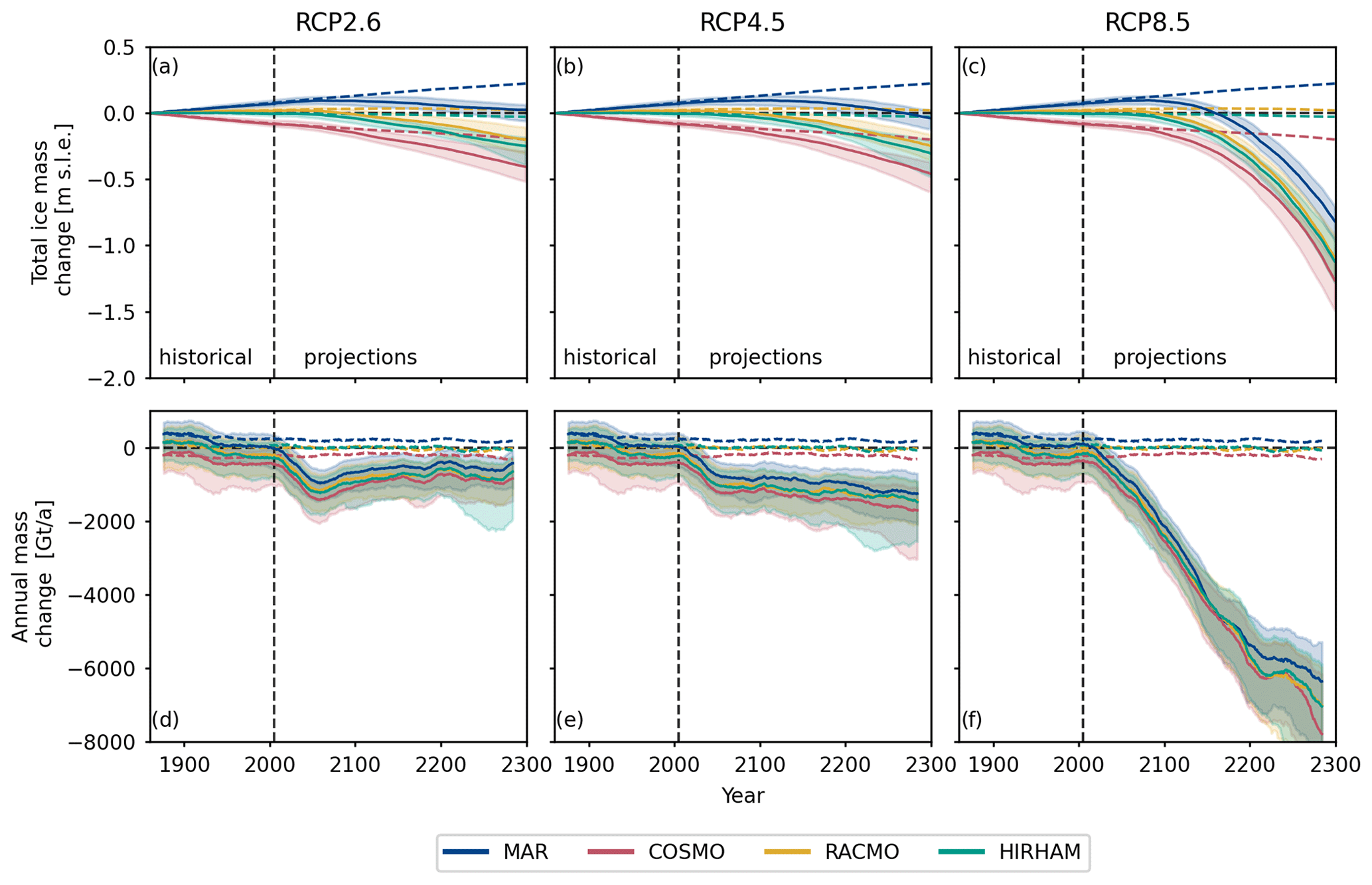
Figure 6 Time series of the median (solid lines) total ice mass above flotation change (a–c) and the annual rate of change (d–f) for the four different RCM forcing fields and the RCP2.6, RCP4.5 and RCP8.5 climate scenarios. Dashed lines represent the median PI-control simulations. Shadings indicate the 5th to 95th quantile.

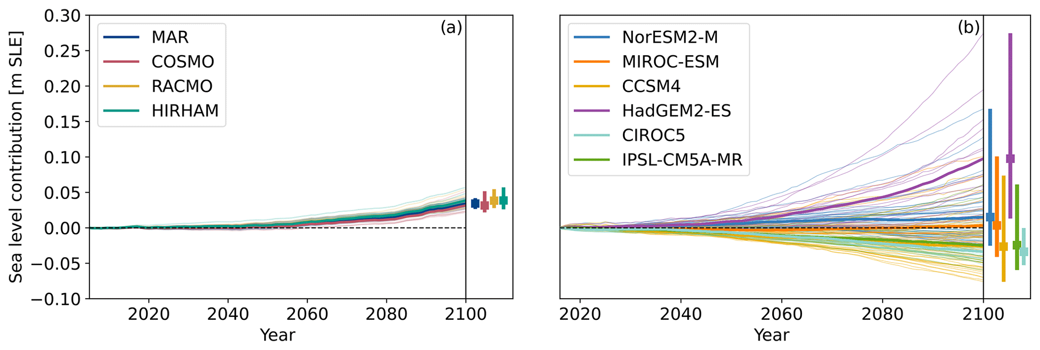
Figure 7 PI-control-corrected Antarctic sea level rise contribution for the RCP8.5 scenario with different RCM present-day fields (a) and from ISMIP6 (Seroussi et al., 2020) (b) until the year 2100. Thin lines show individual simulations, while bold lines show the mean state for the different models. Note that in our study GCM anomalies from HadGEM2-ES (Jones et al., 2018) were used together with RCM forcing fields. We also show a zoomed version of (a) in Fig. C1 and an extension until the year 2300 in Fig. C2.

3.2.1 Imprint of RCM present-day forcing on sea level rise projections

In the following we show the uncertainties in sea level rise projections that arise from the choice of RCM baseline data. Figure 7 illustrates the PI-control-corrected sea level rise contribution of the individual simulations until the year 2100 in the RCP8.5 scenario contrasted with the results from Seroussi et al. (2020). We estimate the maximum difference in sea level rise contribution between simulations with different RCM reference forcings. Therefore, we calculate for every member (par) of the parameter ensemble the maximum sea level contribution difference as follows:

$$\begin{array}{}\text{(4)}& \mathrm{\Delta }{\mathrm{slr}}_{\mathrm{par}}^{\max }=\underset{\mathit{\mu },\mathit{\nu }\in \mathrm{\Omega }}{max}({\mathrm{slr}}_{\mathrm{par}}^{\mathit{\mu }}-{\mathrm{slr}}_{\mathrm{par}}^{\mathit{\nu }}).\end{array}$$

Here, $\mathrm{\Omega }=\mathit{\{}\mathrm{MAR},\mathrm{COSMO},\mathrm{RACMO},\mathrm{HIRHAM}\mathit{\}}$ denotes the list of potential RCM reference forcing. The calculation is carried out on two time series datasets: the raw centennial sea level rise projection and the projection with the respective pre-industrial-control simulation subtracted. The simulated differences in sea level rise can be approximated and decomposed into two components: variations arising solely from differences in the regional climate model (RCM) forcing and variations arising from the interplay between RCM forcing differences and transient anomalies in the global climate model (GCM). In the pre-industrial-control simulations, the GCM anomalies remain constant over time. Consequently, the pre-industrial-control simulation exhibits sea level changes resulting purely from differences in the RCM forcing. By subtracting the pre-industrial-control simulation from the centennial projections, the interplay between RCM forcing differences and GCM anomalies is isolated. This allows for the analysis of how the RCM forcing variations interact with the transient GCM anomalies to influence sea level rise projections.

The resulting Δslr^max for all three RCP scenarios in the PI-corrected (blue) and uncorrected (orange) case are illustrated in Fig. 8 for the year 2100 (Fig. 8a) and 2300 (Fig. 8b). In both cases we only consider differences that arose after 2005. For the year 2100, the PI-control-corrected median Δslr^max is 9.2 mm for the RCP2.6, 10.5 mm for RCP4.5 and 10.6 mm for RCP8.5, which is around an order of magnitude smaller than the uncorrected Δslr^max. The Δslr^max is mostly independent of the projection scenario due to the fact that our simulations only differ minimally until the year 2100 (see Fig. 6). In the year 2300, the PI-control-corrected Δslr^max is around a third of the uncorrected Δslr^max. Additionally, one can observe an increase in the median Δslr^max from 36.1 mm for RCP2.6 to 52.6 mm for RCP4.5 and to 70.0 mm for RCP8.5. Please note the shaded outlier in the PI-control-corrected Δslr^max. This outlier shows the Δslr^max for parameter configuration no. 12 (see Table C1), which shows a partial collapse of the WAIS in the PI-control simulation when forced with COSMO (see Fig. C6). This is further discussed in Sect. 3.2.4. Since this configuration resulted in reasonable PI-control grounding lines for all other RCM forcings, we did not exclude it from our ensemble.

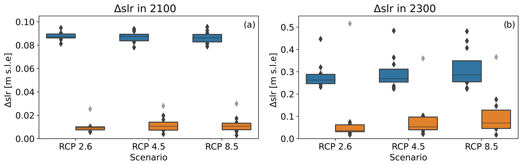
Figure 8 $\mathrm{\Delta }{\mathrm{slr}}_{\mathrm{par}}^{\max }$ in the year 2100 (a) and 2300 (b) for the PI-control-corrected (orange) and uncorrected (blue) case. Boxes indicate the 25th to 75th percentile and the median. Diamonds indicate values outside of the 25th to 75th percentile. The shaded diamonds mark the $\mathrm{\Delta }{\mathrm{slr}}_{\mathrm{par}}^{\max }$ for ensemble configuration no. 12 (see Table C1), which shows a WAIS collapse for the COSMO forcing in the PI-control simulation (see Fig. C6).

3.2.2 Impact of reference RCM on regional ice thickness

The spatial distribution of Δh (thickness deviation from the common mean; see Eq. 3) and the simulated grounding line position at the year 2300 is illustrated in Fig. 9 for Thwaites and Pine Island glaciers and in Fig. C3 for the entire AIS. In all three scenarios a similar ice sheet response is simulated. Simulations forced with MAR generally show higher Δh, especially at Thwaites Glacier (see Fig. 9), along the Transantarctic Mountains and in the Filchner–Ronne Ice Shelf (see Fig. C3). In contrast, simulations forced by COSMO mainly depict negative Δh. Simulations forced by RACMO or HIRHAM show a generally diverging pattern with mostly positive Δh over Thwaites Glacier for HIRHAM and negative for RACMO. In East Antarctica the opposite is observable with positive Δh in simulations forced by RACMO and negative Δh for HIRHAM. Although the overall patterns of ice Δh are rather similar for all three RCP scenarios, major differences in ice thickness are observable at Thwaites Glacier. For MAR simulations, Δh is substantially larger for the RCP8.5 scenario than for the RCP4.5 scenario. On the other hand, COSMO yields a lower Δh for the RCP8.5 than RCP4.5 scenario. The changes in Δh between the RCP4.5 and RCP8.5 scenario are less pronounced for RACMO and HIRHAM, where RACMO and HIRHAM show a decrease and an increase in Δh, respectively.

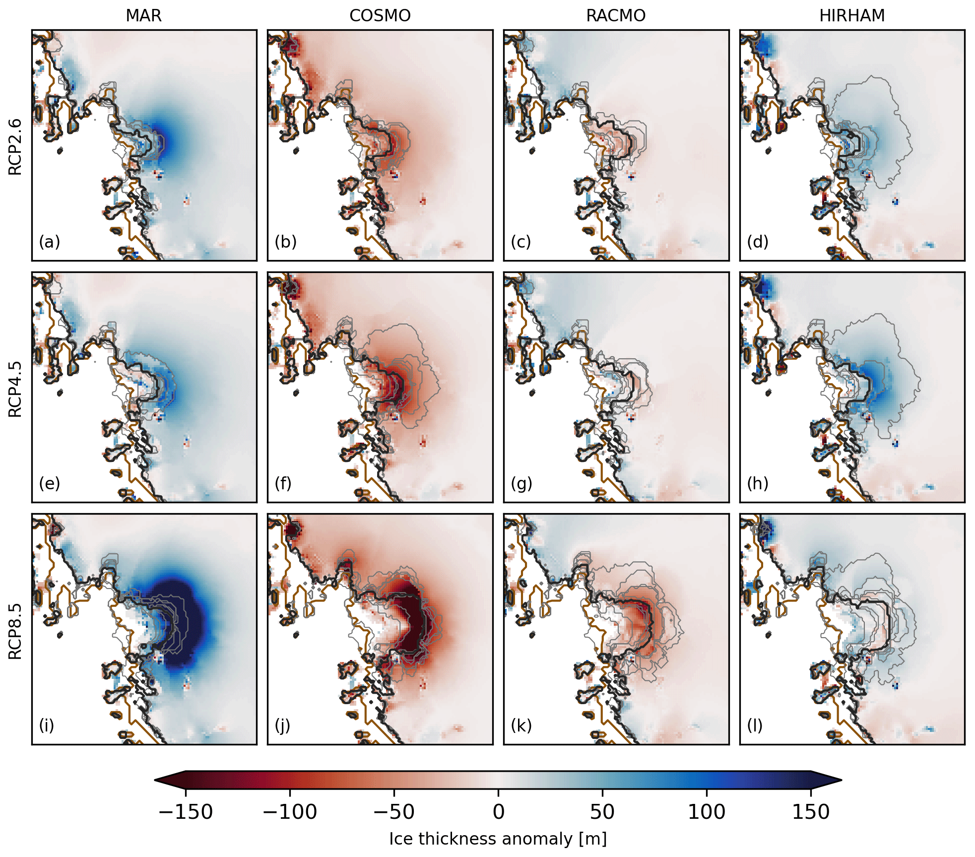
Figure 9 Median ice thickness anomalies from common mean for RCP2.6 (a–d), RCP4.5 (e–h) and RCP8.5 (i–l) together with the position of the simulated median (black) and observed (brown) grounding line at the year 2300. The thin grey lines indicate the simulated grounding line position of the individual ensemble members (see Table C1). Please be aware of the changed color-scale with respect to Fig. 4.

3.2.3 Ensemble sensitivity to reference RCM forcing

The sensitivity of Δh to ice sheet model parameters under a single RCM baseline reference forcing is shown by the root-mean-square deviation (RSMD) depicted in Figs. 10 and C4. This allows the identification of regions where the chosen ice sheet model parameterization has a high impact on simulated ice thickness differences. For for all scenarios the largest parameter sensitivity can be observed at Thwaites and Pine Island glaciers. For the RCP8.5 scenario, the Thwaites and Pine Island glaciers still exhibit the strongest parameter sensitivity. However, the Filchner–Ronne and Ross shelves show significant additional parameter sensitivity. A large Δh does not necessarily also imply a large parameter sensitivity. For example, the Transantarctic Mountains show high absolute Δh values between different baseline models, while the parameter sensitivity is particularly small.

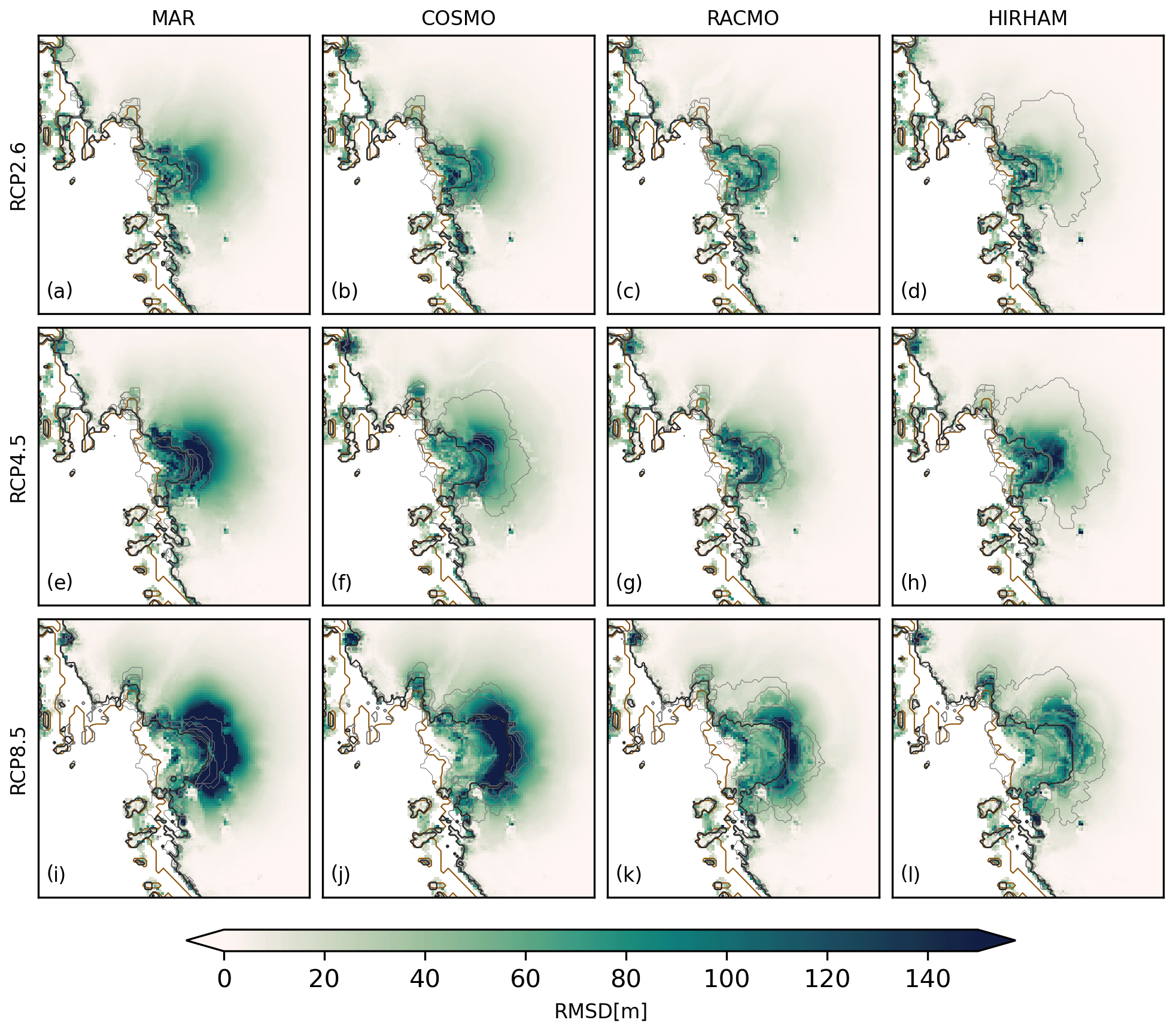
Figure 10 RMSD for RCP2.6 (a–d), RCP4.5 (e–h) and RCP8.5 (i–l) together with the position of the simulated median (black) and observed (brown) grounding line at the year 2300. The thin grey lines indicate the simulated grounding line position of the individual ensemble members (see Table C1). Please be aware that the color scale used in this section is narrower than in the previous sections.

3.2.4 Grounding line sensitivity to RCM baseline forcing

The regional impact (Amundsen Sea sector) of the applied forcings and parameter configuration are illustrated in Figs. 9 and 11. In detail, Fig. 11 illustrates the ensemble statistics of the grounding line position in the Amundsen Sea sector. Percentiles were drawn from the grounded ice mask density, which states, for every grid location (i,j), the percentage of ensemble members that have grounded ice at this location. In our PI-control simulations changes in grounding line positions with respect to the observed grounding line and the spread due to the RCM baseline forcings are rather small. However, a difference between simulations forced by COSMO is observable, especially for the most extreme case (95th percentile). In this case (configuration no. 12), the simulation forced by COSMO shows collapse of WAIS until the year 2300, while there is almost no grounding line retreat in the simulations forced by the other models (see Fig. C6). This is quite remarkable since under the same parameters, the simulation forced with COSMO shows minimal grounding line change for the RCP2.6 scenario (see Fig. C7). While the grounding line position does not significantly change for the least extreme grounding line position (5th percentile) in any of our scenarios, we observe an increase in grounding line retreat within our scenarios for the 50th and 95th percentile of grounding line position. Differences in grounding line position due to the choice of RCM are rather small in the RCP2.6 and RCP4.5 median grounding lines. For the most retreated grounding line (95th percentile), there are large differences between the individual RCM forcings for all scenarios. Please be aware that we show the ensemble statistics of the grounding line extent, which does not necessarily represent a specific parameter configuration. On the level of specific ensemble members, the difference between the individual RCMs tends to be higher (see Figs. C7, C8, C9).

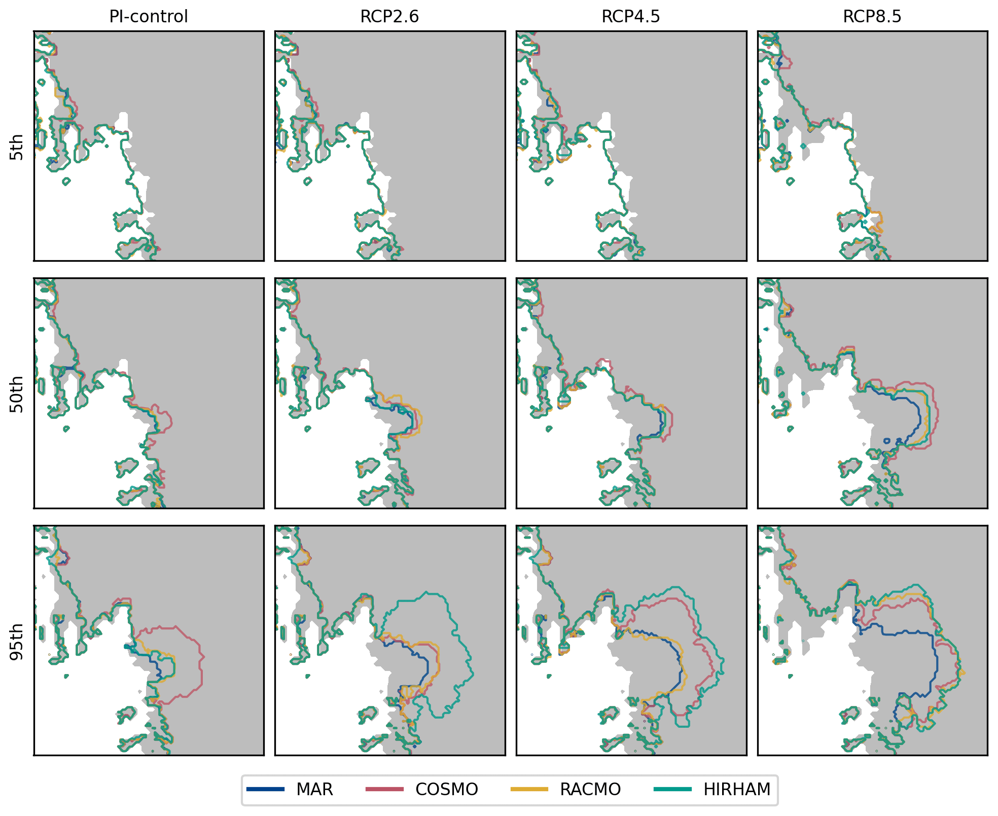
Figure 11 The 5th, 50th and 95th percentile of grounding line position at the year 2300 for simulations using the four RCM forcing sets in the PI-control (a–c), RCP2.6 (d–f), RCP4.5 (g–i) and RCP8.5 (j–l) scenario at the Thwaites and Pine Island glaciers. Percentiles were drawn from the grounded ice mask density, which states, for every grid location (i,j), the percentage of ensemble members that have grounded ice at this location. The grey-shaded area indicates observed present-day grounded ice extent.

4 Discussion

The aim of this modeling study was to quantify and demonstrate the impact of different baseline SMB and temperature forcings on the evolution of the Antarctic Ice Sheet under a 30 000-year present-day equilibrium climate and projections using RCP scenarios extended to the year 2300. We now discuss the modeled future sea-level rise contributions and their uncertainties, ice sheet stability, and equilibrium states under present-day forcing.

4.1 Uncertainty in Antarctic sea level contributions due to the choice of RCM baseline forcing

Our simulations suggest differences in projected Antarctic sea level contributions due to the choice of present-day SMB and temperature baseline forcing of 10.6 (2.9–30.0) mm in 2100 and 70.0 (17.3–365.5) mm in 2300 for RCP8.5 if we correct them using the PI-control simulations. Those numbers are around a factor of 10 (for 2100) and 3 (for 2300) smaller than without the PI-control corrections. Since we often assume Antarctica has been stable during the Holocene, the base RCM forcing should not yield any changes under PI conditions. This leads us to the conclusion that the interplay between the RCM and the GCM anomalies (PI-corrected Δslr^max) is the more accurate estimate of RCM-induced uncertainties in centennial projections. In comparison to our results, the ISMIP6 project demonstrated that the choice of ISM and GCM forcing creates an uncertainty spread of 13.3±8.0 cm SLE (projections ranging from $-\mathrm{3.7}\pm \mathrm{3.4}$ to 9.6±7.2 cm SLE) for the end of the 21st century under the RCP8.5 scenario (Seroussi et al., 2020). Our estimates of RCM uncertainties are over an order of magnitude smaller, and therefore they probably only play a small role in projections until the year 2100. Nevertheless, the ISMIP6 ocean forcing induces a sea level rise projection spread by 2100 between 1.4–4.0 cm (Reese et al., 2020) with the same ISM used in this study. Additionally, we do not observe significant differences in Δslr^max between different RCP scenarios in 2100. This is probably because differences between those RCP scenarios will not become apparent until after the 21st century, as noted by Lowry et al. (2021). For the year 2300, results for the extended ISMIP6 simulations are not yet publicly available. However, based on our results, we expect the importance of the RCM uncertainty to increase, since the relation between PI-corrected and uncorrected Δslr^max increases 3-fold from 2100 to 2300 (see Fig. 8). The increase in Δslr^max from the RCP2.6 to RCP8.5 scenario additionally suggests that the RCM-induced uncertainty might be larger for stronger warming scenarios. Nevertheless, projections by Bulthuis et al. (2019) show a parameter-choice-dependent spread in projected sea level rise from 0.17–3.12 m (5 %–95 % confidence interval), compared to which our estimated impact of RCM choice seems to be rather small. Nevertheless, the parameter uncertainties by Bulthuis et al. (2019) may be considered an upper limit compared to other studies (Golledge et al., 2015; Ritz et al., 2015; DeConto and Pollard, 2016; Schlegel et al., 2018). It is important to note that the uncertainty presented here depends partly on the initialization method and the GCM forcing applied. In contrast to this study, in the ISMIP6 protocol models were initialized with different reference present-day forcing fields. Furthermore, various types of model tuning were applied to match present-day observations, e.g., nudging or inversion (Seroussi et al., 2020; Nowicki et al., 2020). Specifically, initialization techniques, such as basal friction inversion or nudging, have the capability to incorporate substantial portions of the reference forcing differences into the refined basal friction field. While this could reduce model deviations from the observed state of the ice sheet, it might concurrently give rise to larger differences in a changing climate. Notably, the WAIS is especially sensitive to these minor discrepancies in basal friction due to its overall high sensitivity, particularly because of the marine ice sheet instability (MISI) (DeConto and Pollard, 2016).

4.2 Choice of RCM baseline affects the stability of the WAIS in future projections

The complex relationship between the selected RCM baseline climatology and its impact on future sea level rise is closely related to the stability of WAIS, particularly the dynamic response of Thwaites and Pine Island glaciers. This becomes particularly evident in the context of the RCP8.5 scenario. Depending on the choice of RCM, the baseline forcing differences in grounding line migration (see Fig. 11) and the corresponding ice thickness changes (see Fig. 9) are simulated. This underscores the WAIS's sensitivity to the choice of present-day reference forcing data and underlines the importance of careful model parameterization and selection of forcing data. It is important to note that the reference forcing data do not influence whether the WAIS enters a grounding line retreat in our centennial projections but rather modulates the rate of ice loss (see Fig. C9). The initiation of unforced grounding line retreat seems to be predominantly dependent on the ocean thermal forcing. This is evident from the fast ice loss observed soon after the beginning of the RCP8.5 scenario, which is in stark contrast to the control runs that mostly exhibit minimal changes (see Fig. 6).

4.3 Millennial-scale response predisposed by choice of RCM reference forcing

To demonstrate the influence of reference SMB and temperature fields on the long-term evolution of WAIS, we presented individual simulation results from our ensemble, as shown in Fig. 5. Our simulations indicate that differences in reference SMB and temperature forcing can lead to not only a slow, gradual response of the ice sheet thickness but also to centennial-scale, nonlinear responses. When constant COSMO and MAR forcing is applied for identical ice sheet model parameters, a collapse of the WAIS is observed (see Fig. 5), while exactly the same parameters yield a stable WAIS under RACMO and HIRHAM forcing. In those simulations forced by MAR and COSMO, individual grid boxes unground, as shown in Fig. B5, which leads to accelerated ice flow. Notably, the long-term evolution of the ice sheets might also be affected by the thermal spinup. In this study, we only performed a thermal spinup using the constant PD temperature fields. Therefore, we might lack the historical temperature imprint of the last glacial cycles in the ice sheet, which might affect dynamics, especially when the configuration is close to an instability. Additionally, several of our simulations do not seem to have reached a (quasi-)steady state after 30 kyr. We therefore can not exclude a potential WAIS collapse at a later stage (i.e., after the initial 30 kyr of our simulations). This would imply that the committed ice sheet response is mainly driven by the parameter set itself, while the RCM climatology might modulate the timing of the collapse. However, this hypothesis would require longer simulations that are beyond the scope of this study.

4.4 SMB anomalies are imprinted in ice thickness equilibrium

The simulated change in sea-level-relevant ice mass in the present-day equilibrium simulations demonstrates the expected behavior, where simulations with the highest SMB forcing (e.g., MAR) lead to the largest ice volume (see Fig. 3). The observed spatial distributions of Δh roughly agree with the anomalies observed in the SMB forcing. Regional-scale structures in Δh often differ from the underlying SMB anomalies, perhaps unsurprisingly given the inherent nonlinearities of WAIS dynamics. Here we discuss the relationship between regional SMB forcing and the quasi-equilibrium state of the ice sheet for individual catchment areas (i.e., IMBIE basins; Rignot et al., 2011). Averaged over those basins (see Figs. A2, B2), the ice sheet responds in line with the SMB forcing with only a few exceptions. One exception is the WAIS in simulations forced with the SMB and temperature fields from RACMO. While we mostly observe small positive SMB anomalies with respect to the RCM mean for all WAIS basins except the Ross basin, the thickness anomalies (Δh) are all negative for those basins. The reason for this might be a shift in the ice divide, which would result in an outflux of ice towards the Ross drainage basin. However, a more in-depth analysis would be necessary to assess if this is the main driver of the observed behavior. In addition, one has to note that our study did not account for any ice sheet feedbacks of the ice thickness change on surface temperature and mass balance, which might lead to a different result (Coulon et al., 2024; Li et al., 2023).

4.5 Parameter sensitivity of the RCM impact

The ice-sheet-wide parameter sensitivity of Δh is larger for the present-day equilibrium simulations than in the centennial projections. This can be attributed to the long response time of the AIS, especially in vast areas of the East Antarctic Ice Sheet (EAIS), and the much smaller simulation time in the future projections. However, for the Thwaites and Pine Island glaciers, the parameter sensitivity of Δh is higher in the centennial projections. This can be explained by the fact that the present-day forcing exposes the Antarctic Ice Sheet (AIS) to weaker climate drivers (e.g., ocean-induced melt) than all of the RCP scenarios. Therefore, we would expect the parameter sensitivity of Δh to be more similar to the RCP2.6 than the RCP8.5 scenario. Generally, a high parameter sensitivity of Δh highlights regions where the interplay between SMB and chosen parameters is highest. Therefore, the model representation of these regions would especially benefit from a better constrained surface mass balance forcing.

5 Conclusion

Regional climate model SMB and temperature data are a standard resource for studies employing large-scale ISMs. In this study, we investigated the influence of a set of different RCM products on the evolution and dynamics of the AIS in 30 000-year constant forcing equilibrium simulations and in several future projections employing RCP2.6, RCP4.5 and RCP8.5 using a parameter ensemble reflecting various ice sheet sensitivities. Our results demonstrated that although all surface mass balance and temperature products are externally driven by the same reanalysis and simulate the same fields, the impact of their differences on both ice thickness and grounding line dynamics is considerable. For the long-term “quasi-equilibrium” state after 30 kyr of simulation, we showed that ice thickness anomalies averaged over the individual IMBIE drainage basins mostly reflect SMB differences between RCMs. However, the differences in SMB forcing can lead to nonlinear ice sheet responses on regional scales. For the centennial-term projections, our findings indicate that differences mostly arise in, and are limited to, the vicinity of the grounding line. Our simulations further show that the model uncertainty for sea level rise projections coming from the difference in reference present-day forcing is around 10 % of the uncertainty arising from the choice of ISM and GCM forcing based on ISMIP6 results. However, the RCM uncertainty seems to increase for longer projections and higher-emission scenarios. Additionally, our simulations depict differences in the pacing and timing of grounding line retreat and ice thickness for Thwaites and Pine Island glaciers under all emission scenarios. Our sensitivity analysis indicates that the imprint of the SMB forcing on the ice thickness is especially dependent on the chosen parameters for the ISM (model sensitivity). Our long-term equilibrium study additionally indicates that the difference in the SMB products is potentially large enough to result in long-term instabilities of the WAIS in one forcing set, while long-term WAIS stability can be observed in another. Our study displays the large impact of the choice of a reference present-day forcing onto projections of ice sheet evolution; however, this sensitivity is model dependent and should be explored on a case-by-case basis. Prospectively, a more rigorous approach employing a wider sweep of parameters, more sophisticated ice sheet initialization methods (less model drift), and a larger set of GCM and RCM climate projections would be desirable. However, we demonstrate here that the problem occurs due to the spread in RCM products, the order of magnitude of this uncertainty and potential implications on the stability of the ice sheet.

Appendix A: Annual SMB in the different drainage areas

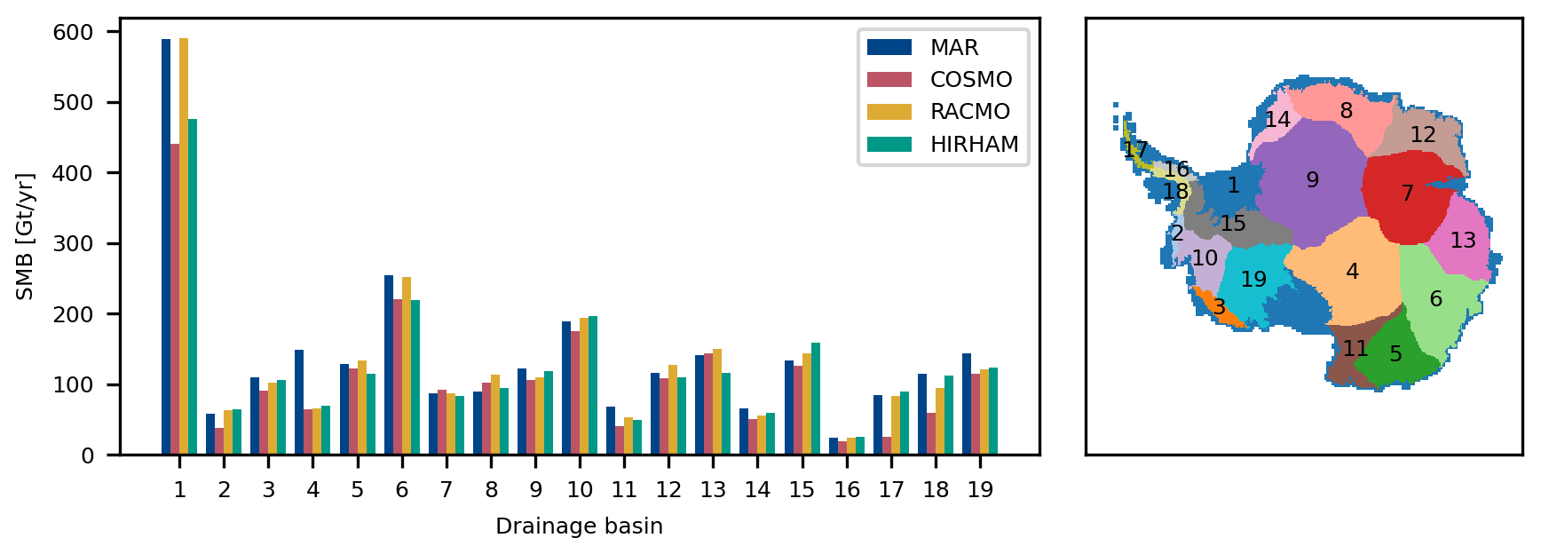
Figure A1 Annual SMB for the 19 IMBIE drainage areas. Corresponding areas are marked on the map. Please be aware that area 1 includes all shelf ice areas.

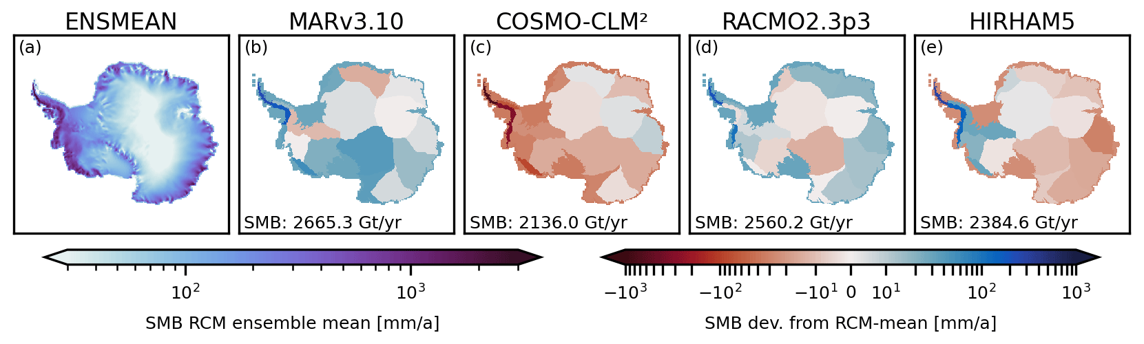
Figure A2 Surface mass balance (SMB) of the (a) multi-RCM mean and anomalies of the (b) MARv3.10, (c) COSMO-CLM2, (d) RACMO2.3p3 and (e) HIRHAM5 regional climate model from this mean averaged over the individual IMBIE basins.

Appendix B: Ice thickness difference from PD observations for PD equilibrium

Table B1 Chosen parameter space for the shallow ice approximation enhancement factor sia_e, the pseudo-plastic pQ factor, the heat conductivity at the ice–ocean interface γ and the minimum till friction angle ϕ_{till min} for the present-day equilibrium runs.

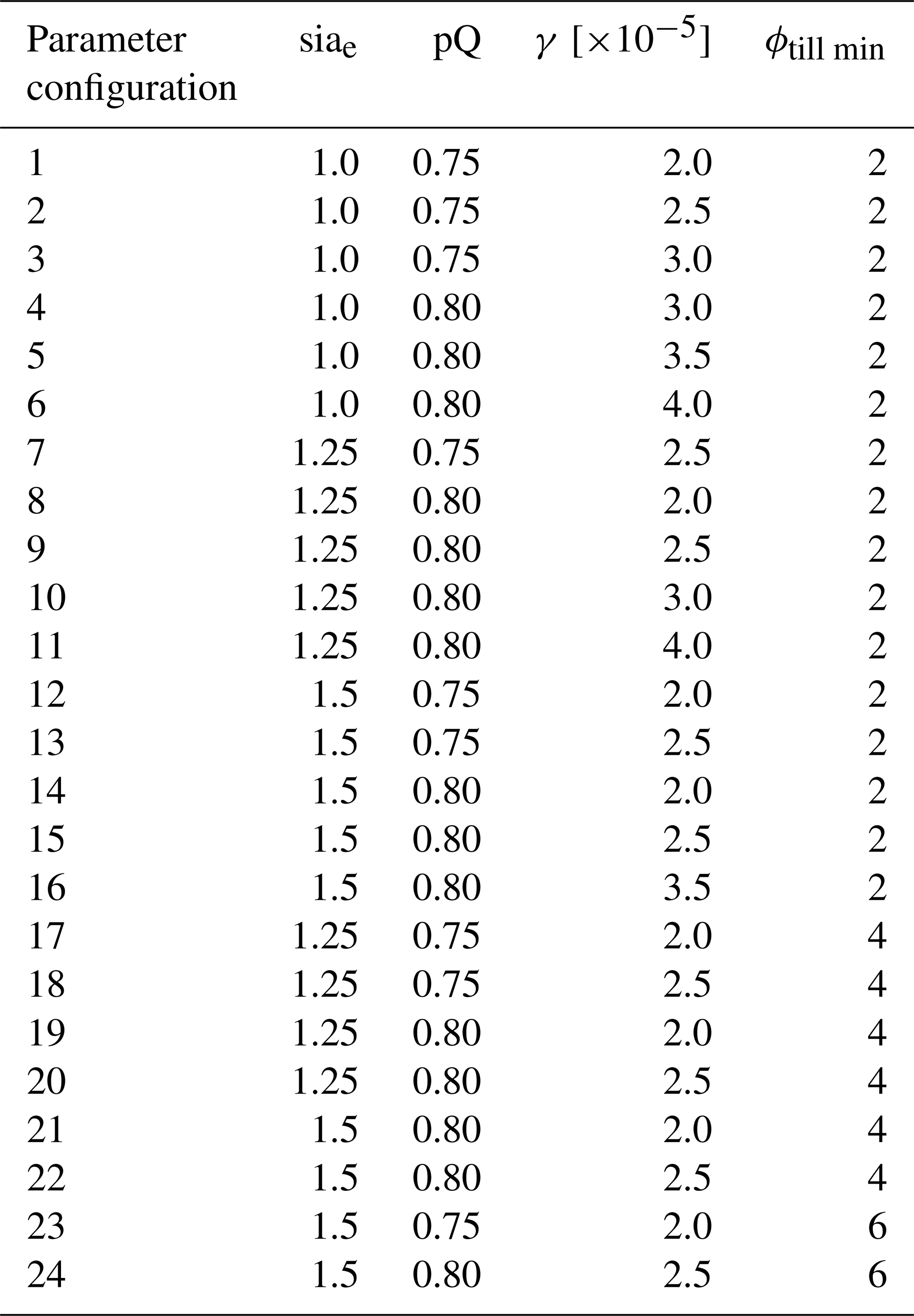
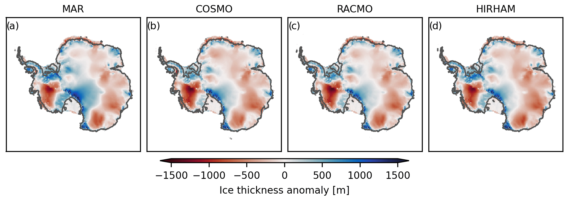
Figure B1 Median ice thickness anomalies compared to present-day observations after 30 000 years under the given RCM SMB.

Table B2 Simulation setups for present-day equilibrium and future projections. B1 and D1 refer to the parameter configurations stated in Tables B1 and C1. The description indicates if the run is a thermal spinup (TS) under which the ice geometry is keep constant or the ice can freely evolve (FE). For the historical simulations, HadGem2-ES anomalies compared to present-day values from 1860 to 2005 are applied. For the RCP scenarios, HadGem2-ES anomalies compared to present-day values from 2005 to 2300 are applied.

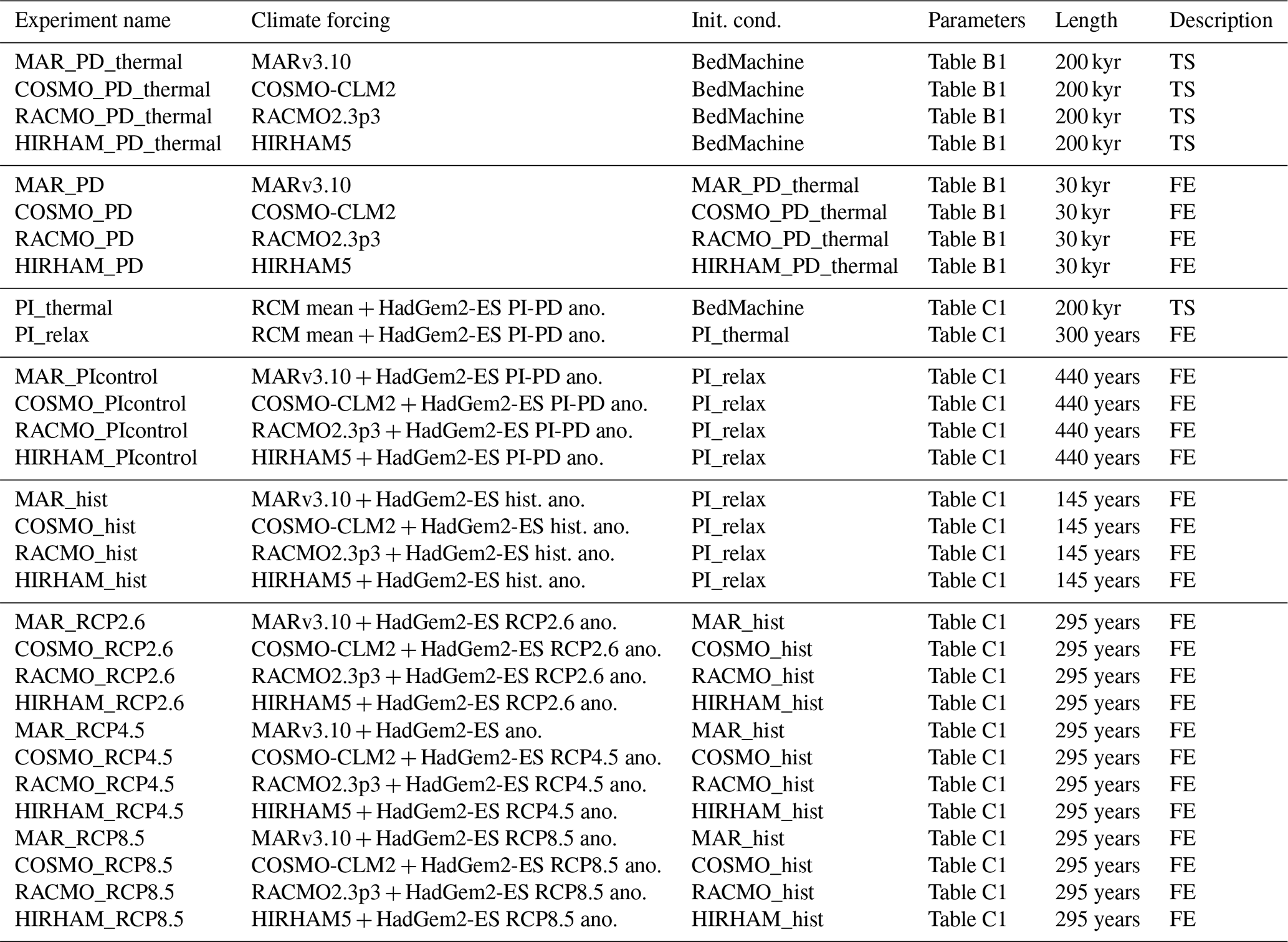
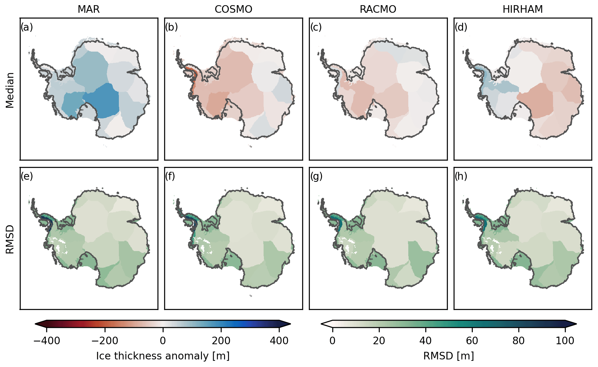
Figure B2 Ice thickness anomalies from the common mean (a–d), position of the simulated (purple) and observed (grey) grounding line for the present-day equilibrium simulations. Root-mean-square difference (RMSD) of the individual ensemble members from the median (e–h). All values are averaged over the individual IMBIE drainage basins.

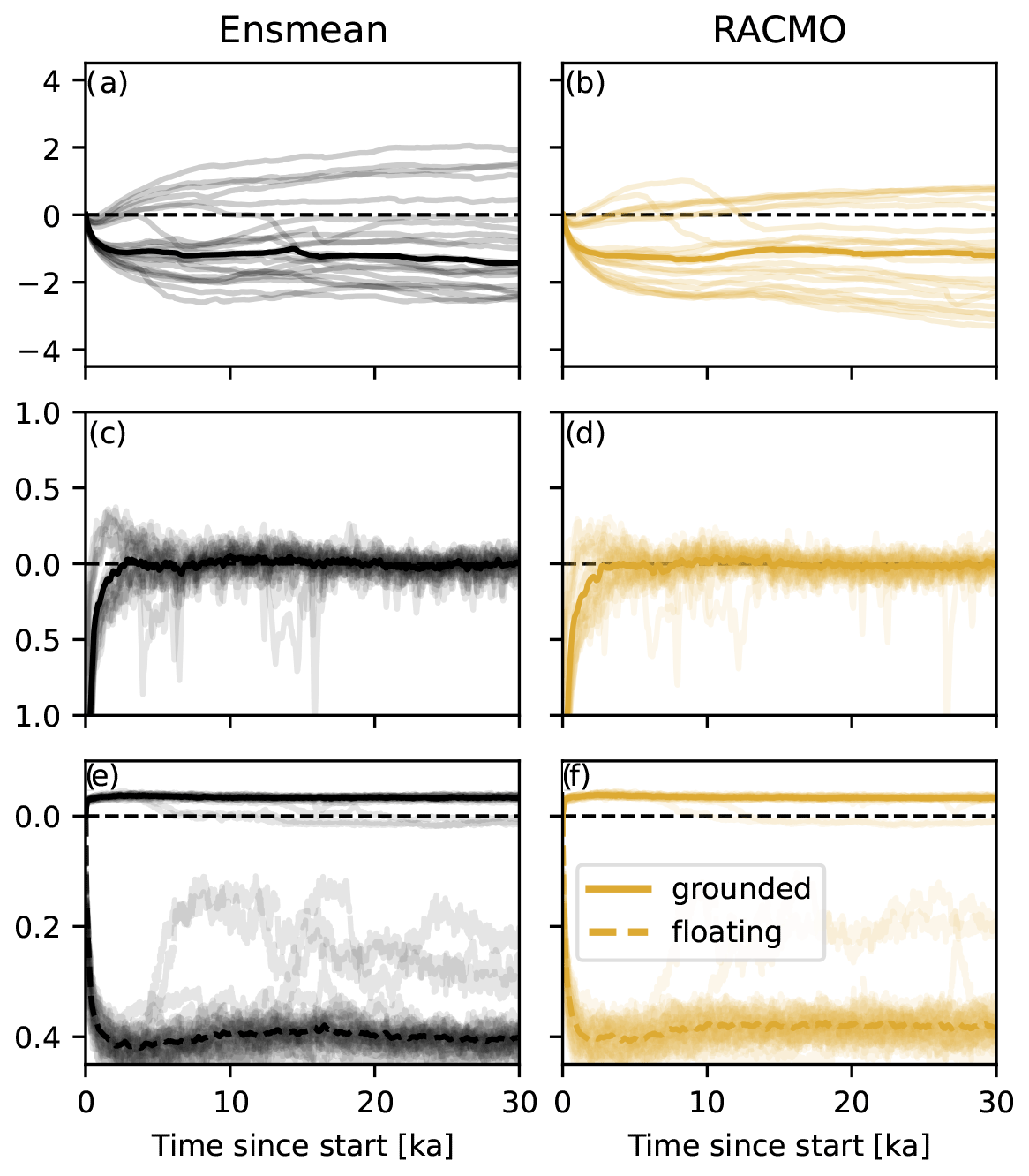
Figure B3 Time series of the total ice mass change (a, b), the annual rate of change (c, d), and the fraction of grounded (solid line) and floating (dashed line) ice area (e, f) relative to present-day observations for the simulations forced by the mean of all four RCM products (referred to as ensmean) and simulations forced by RACMO. The bold line shows the ensemble median, while the shaded lines indicate the individual ensemble members.

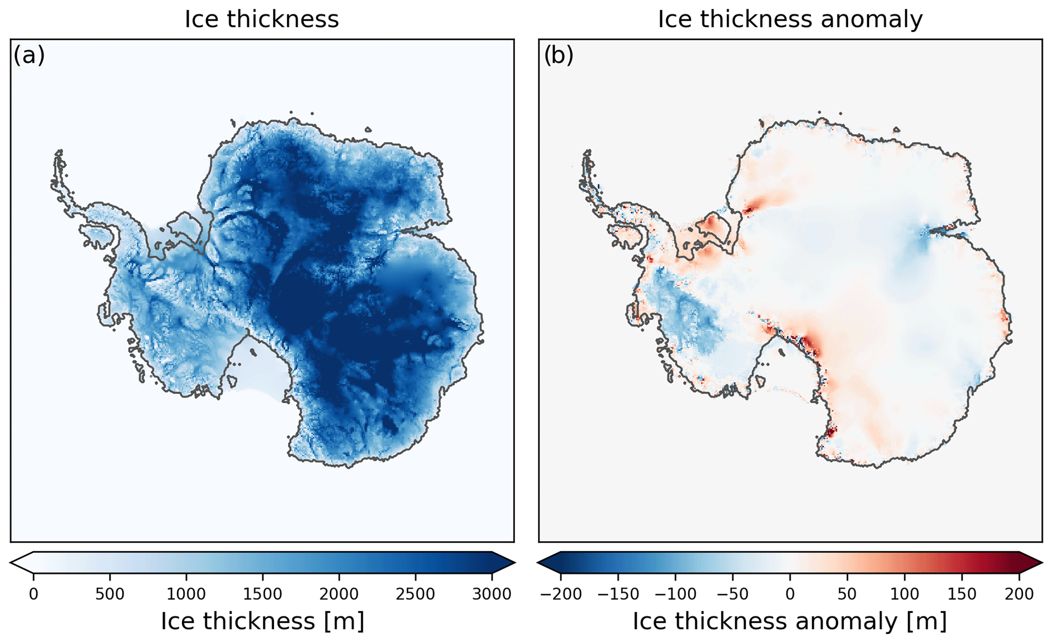
Figure B4 Mean ice thickness after 30 000 years for a simulation forced with the mean of all four RCMs (a) and the mean ice thickness anomalies between those in (a) and the mean of the individual forcing simulations (b).

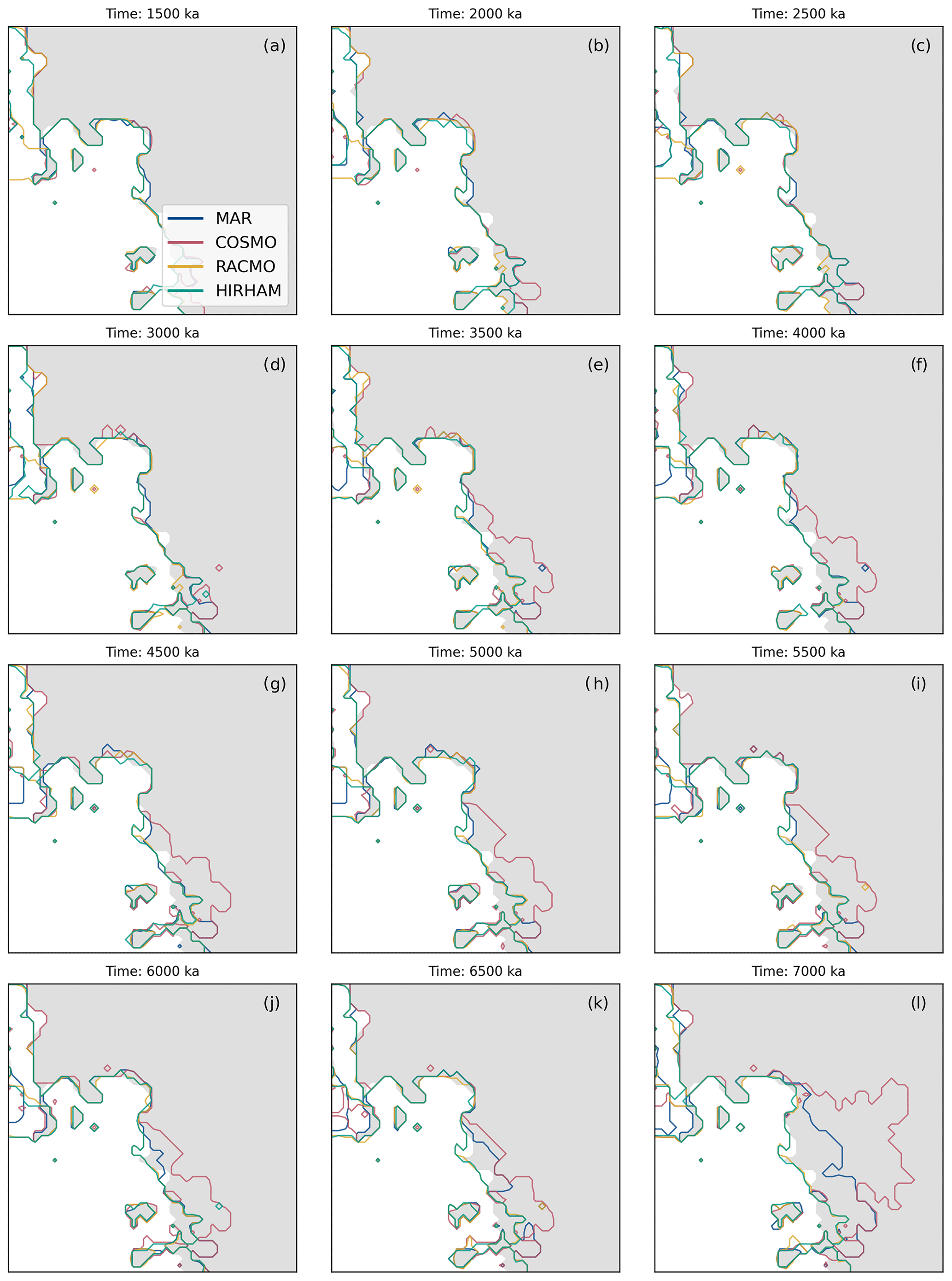
Figure B5 Evolution of the grounding line at Thwaites Glacier for PD parameter configuration no. 6 in time steps of 500 years. The grey-shaded patches represent the present-day grounding line position. The plot indicates that an early grounding line retreat of the simulation forced by the COSMO and later by the MAR model leads to an accelerating retreat of the grounding line, causing the later collapse of WAIS in this simulation, as seen in Fig. 5.

Appendix C: Future projections

Table C1 Chosen parameter space for the shallow ice approximation enhancement factor sia_e, the pseudo-plastic pQ factor, the heat conductivity at the ice–ocean interface γ and the minimum till friction angle ϕ_{till min} for the centennial projections.

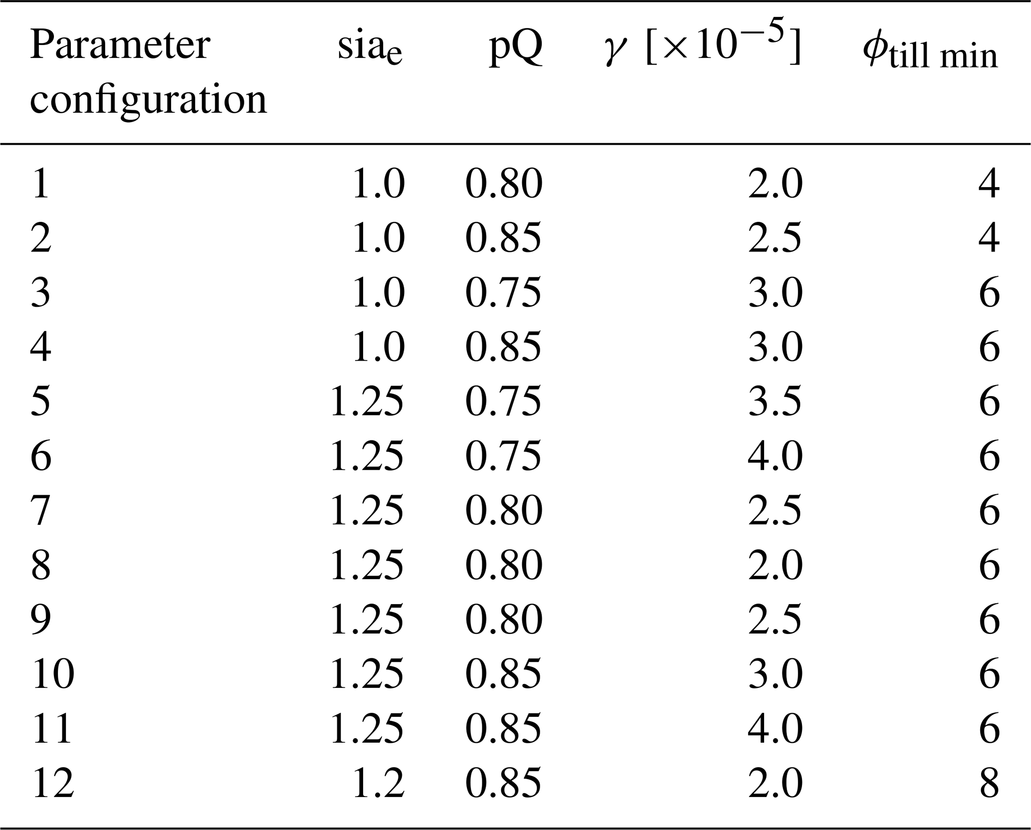
Table C2 Ensemble mean, maximum and minimum total ice mass change from 2015 until 2100 in the PI-control simulations.

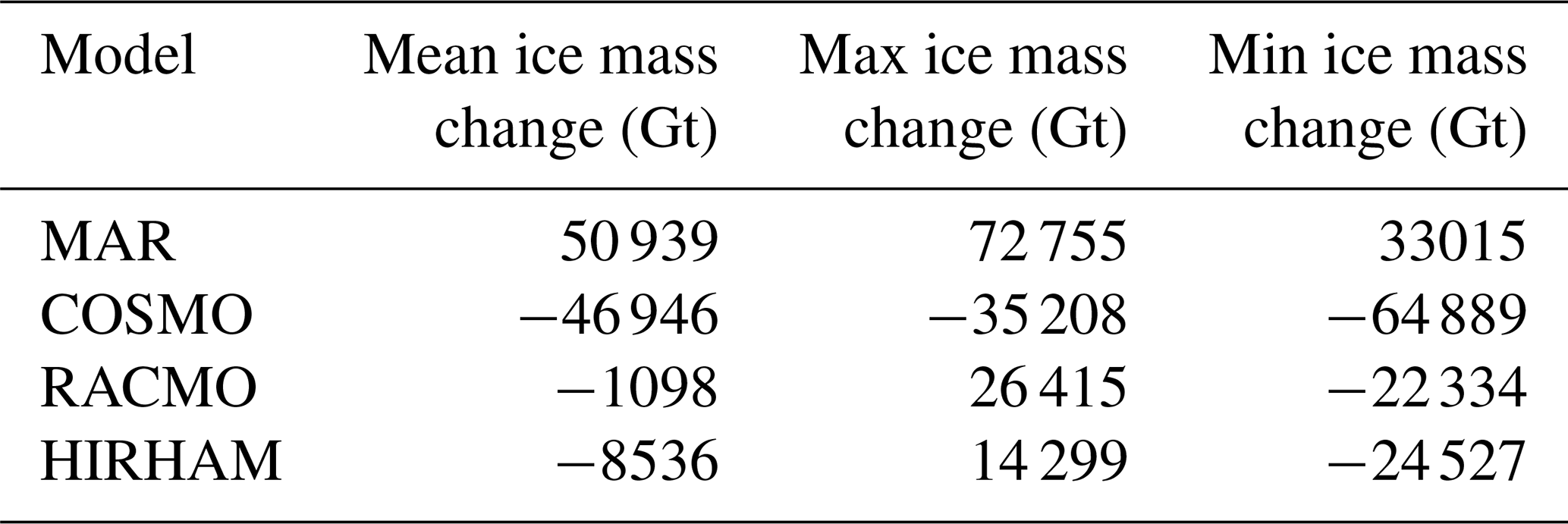
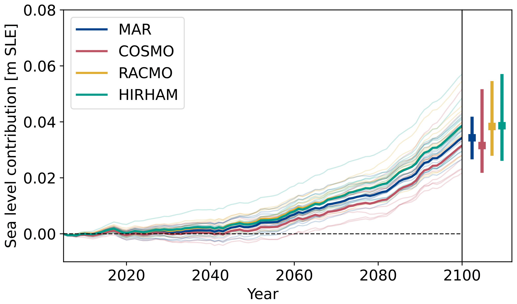
Figure C1 Antarctic sea level rise contribution for the RCP8.5 scenario with different RCM present-day fields until the year 2100. Thin lines show individual simulations, and bold lines show the mean state for the different models.

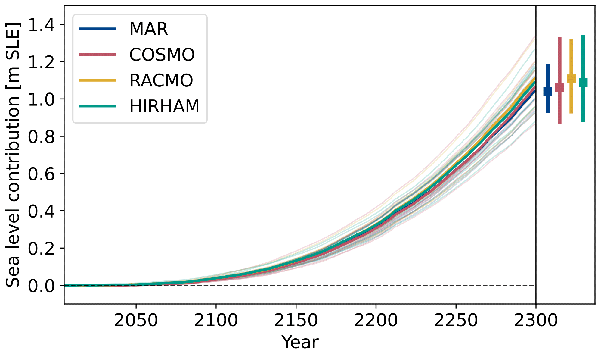
Figure C2 Antarctic sea level rise contribution for the RCP8.5 scenario with different RCM present-day fields until the year 2300. Thin lines show individual simulations, while bold lines show the mean state for the different models.

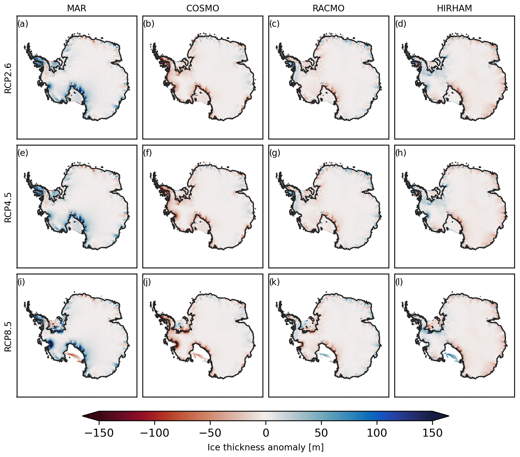
Figure C3 Median ice thickness anomalies from common mean for RCP2.6 (a–d), RCP4.5 (e–h) and RCP8.5 (i–l) together with the position of the simulated median (black) and observed (brown) grounding line at the year 2300. The thin grey lines indicate the simulated grounding line position of the individual ensemble members. Please be aware that the color scale used in this section is smaller than in the previous sections.

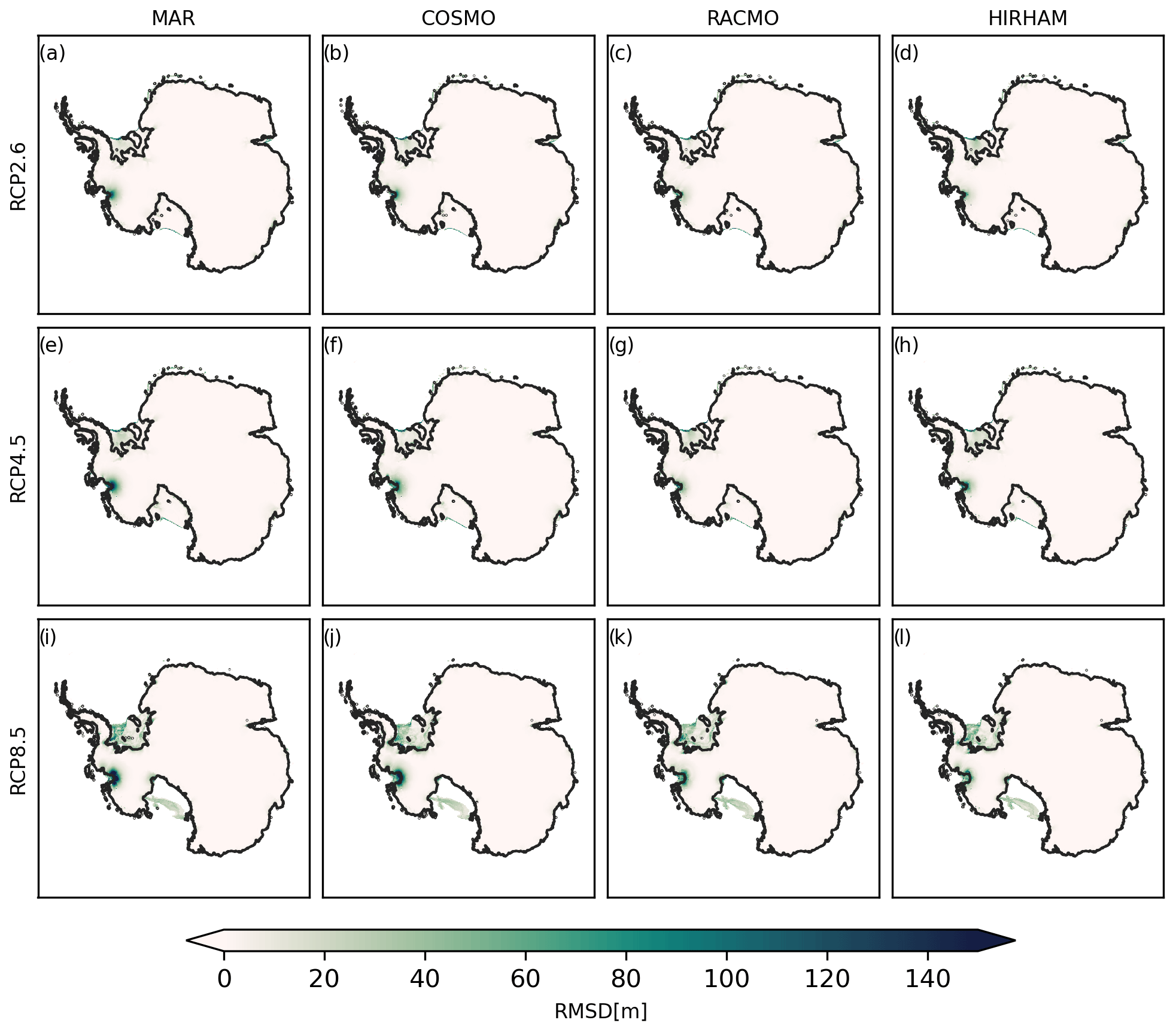
Figure C4 RMSD for RCP2.6 (a–d), RCP4.5 (e–h) and RCP8.5 (i–l) together with the position of the simulated median (black) and observed (brown) grounding line at the year 2300. The thin grey lines indicate the simulated grounding line position of the individual ensemble members. Please be aware that the color scale used in this section is smaller than in the previous sections.

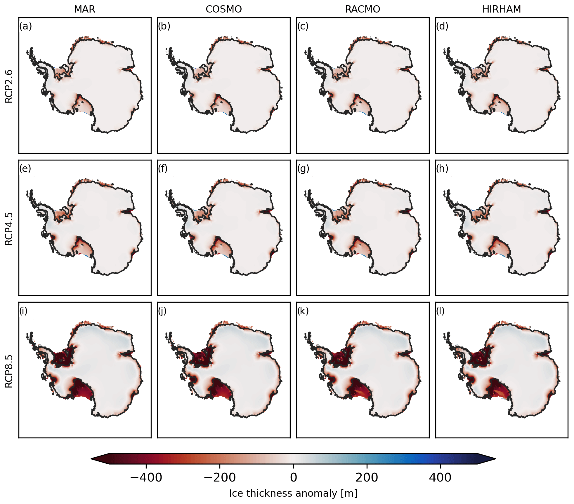
Figure C5 Median ice thickness anomalies with respect to the PI-control simulations for RCP2.6 (a–d), RCP4.5 (e–h) and RCP8.5 (i–l) together with the position of the simulated median (black) grounding line at the year 2300.

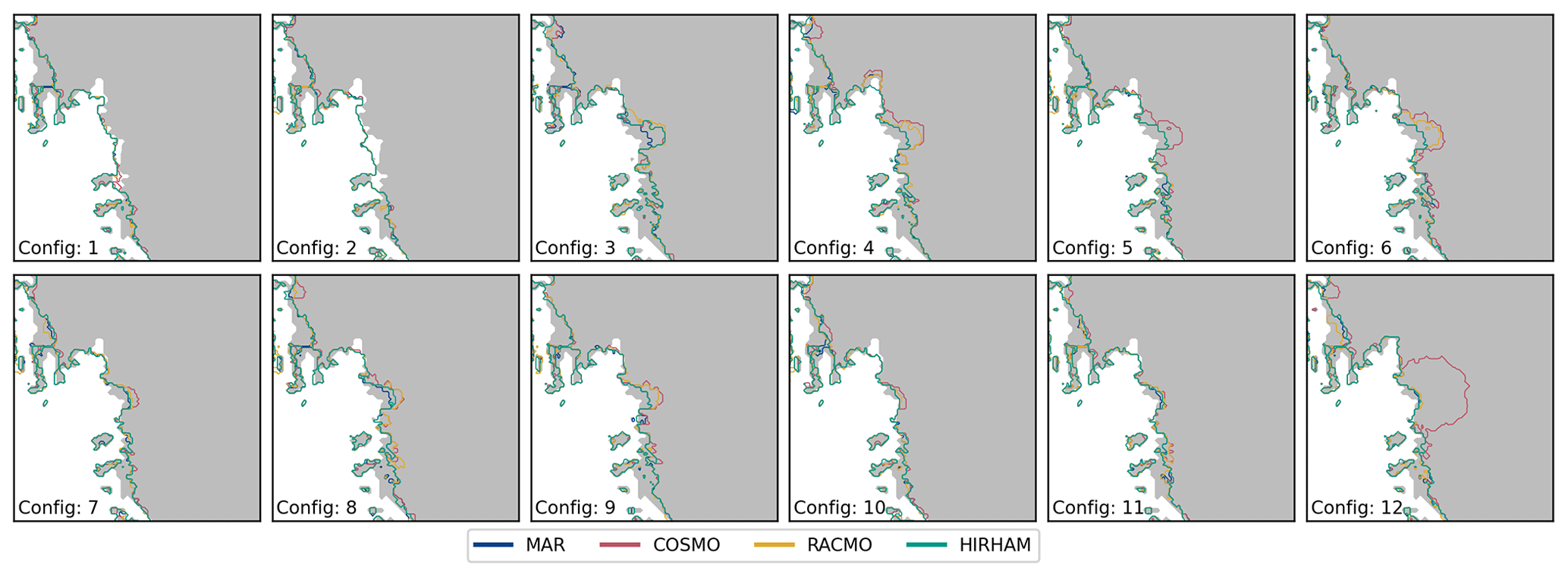
Figure C6 Individual grounding line extent for each individual RCM forcing and parameter configuration (see Table C1) for the PI-control scenario at the year 2300.

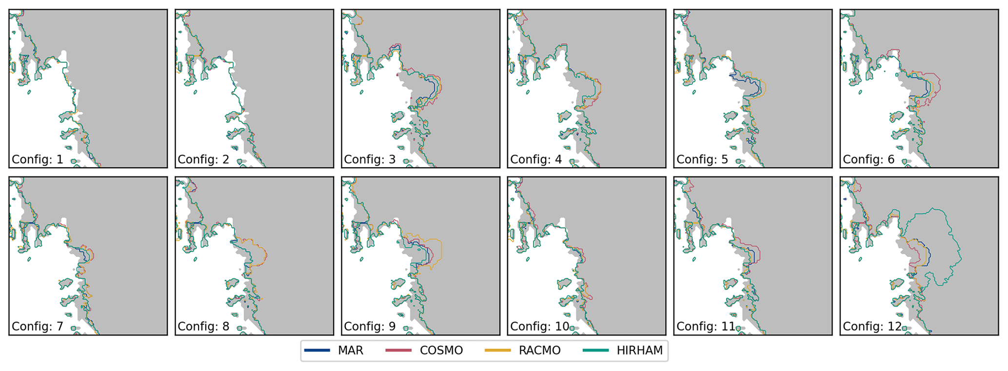
Figure C7 Individual grounding line extent for each individual RCM forcing and parameter configuration (see Table C1) for the RCP2.6 scenario at the year 2300.

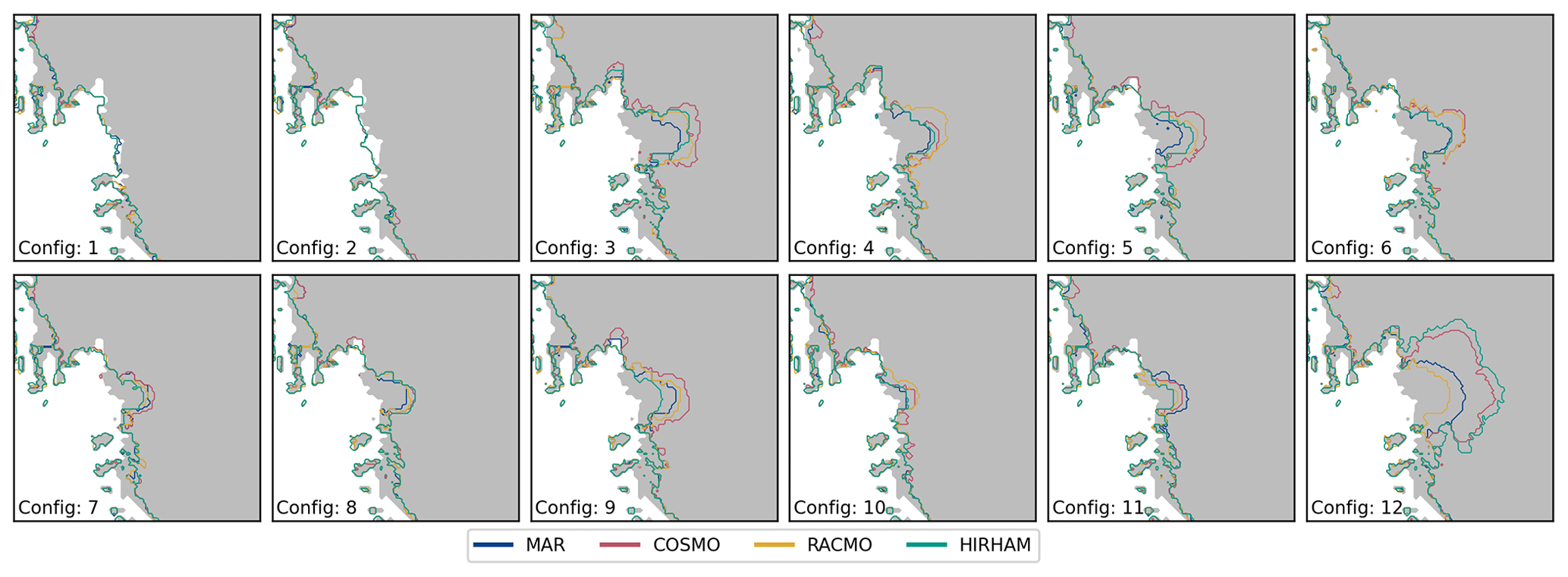
Figure C8 Individual grounding line extent for each individual RCM forcing and parameter configuration (see Table C1) for the RCP4.5 scenario at the year 2300.

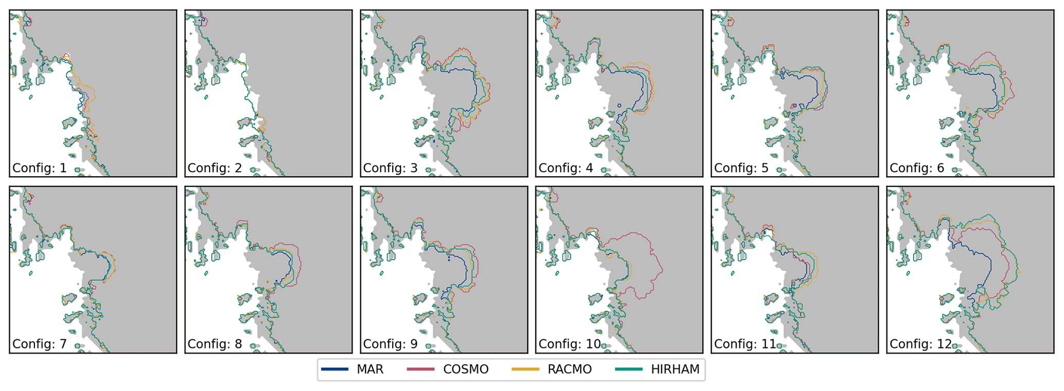
Figure C9 Individual grounding line extent for each individual RCM forcing and parameter configuration (see Table C1) for the RCP8.5 scenario at the year 2300.