Employing automated electrical resistivity tomography for detecting short- and long-term changes in permafrost and active-layer dynamics in the maritime Antarctic

Repeated electrical resistivity tomography (ERT) surveys can substantially advance the understanding of spatial and temporal freeze–thaw dynamics in remote regions, such as Antarctica, where the evolution of permafrost has been poorly investigated. To enable time-lapse ERT surveys in Antarctica, an automated ERT (A-ERT) system is required, as regular site visits are not feasible. In this context, we developed a robust A-ERT prototype and installed it at the Crater Lake CALM-S site on Deception Island, Antarctica, to collect quasi-continuous ERT measurements. We developed an automated data processing workflow to efficiently filter and invert the A-ERT datasets and extract the key information required for a detailed investigation of permafrost and active-layer dynamics.

In this paper, we report on the results of two complete year-round A-ERT datasets collected in 2010 and 2019 at the Crater Lake CALM-S site and compare them with available climate and borehole data. The A-ERT profile has a length of 9.5 m with an electrode spacing of 0.5 m, enabling a maximum investigation depth of approximately 2 m. Our detailed investigation of the A-ERT data and inverted results shows that the A-ERT system can detect the active-layer freezing and thawing events with high temporal resolution. The resistivity of the permafrost zone in 2019 is very similar to the values found in 2010, suggesting the stability of the permafrost over almost 1 decade at this site. The evolution of thaw depth exhibits a similar pattern in both years, with the active-layer thickness fluctuating between 0.20–0.35 m. However, a slight thinning of the active layer is evident in early 2019, compared to the equivalent period in 2010.

These findings show that A-ERT datasets, combined with the new processing workflow that we developed, are an effective tool for studying permafrost and active-layer dynamics with very high resolution and minimal environmental disturbance. The ability of the A-ERT setup to monitor the spatiotemporal progression of thaw depth in two dimensions, and potentially in three dimensions, and to detect brief surficial refreezing and thawing of the active layer reveals the significance of the automatic ERT monitoring system to record continuous resistivity changes. An A-ERT monitoring setup with a longer profile length can investigate greater depths, offering effective monitoring at sites where boreholes are costly and invasive techniques are unsuitable. This shows that the A-ERT setup described in this paper can be a significant addition to the Global Terrestrial Network for Permafrost (GTN-P) and the Circumpolar Active Layer Monitoring (CALM) networks to further investigate the impact of fast-changing climate and extreme meteorological events on the upper soil horizons and to work towards establishing an early warning system for the consequences of climate change.

1 Introduction

Antarctica is home to 90 % of the world's ice, making it a crucial influencer of the Southern Hemisphere and global atmospheric and cryospheric systems (Bockheim, 2004). An understanding of the distribution and properties of Antarctic permafrost is essential for the cryospheric sciences, as well as for ecology and biological sciences, since it is a major control on ecosystem modification following climate-induced changes (Vieira et al., 2010). Despite its significance and compared with other components of the cryosphere, our understanding of Antarctic permafrost and its response to global change remains limited (Biskaborn et al., 2019; Hrbáček et al., 2023). This gap in permafrost knowledge holds true for much of Antarctica, excluding, perhaps, the McMurdo Dry Valleys (MDVs), which have been the focus of substantial research efforts for several decades (Vieira et al., 2010). Systematic investigations on permafrost are less common in other Antarctic regions, and the majority of studies have been conducted in the vicinity of research stations. The harsh climate, environmental conditions, remoteness, and logistical difficulties and expenses impose limitations on permafrost research in Antarctica (Hrbáček et al., 2023).

In the framework of the Global Terrestrial Network for Permafrost (GTN-P), three critical permafrost parameters have been designated as essential climate variables (ECVs) by the Global Climate Observing System (GCOS) of the WMO: (i) the active-layer thickness (ALT), representing the annual thaw depth above permafrost, with a primary focus on data gathered from the Circumpolar Active Layer Monitoring (CALM) network (Brown et al., 2000); (ii) the thermal state of permafrost (TSP), encompassing permafrost temperature, systematically observed through an extensive network of boreholes over the long term (Biskaborn et al., 2019); and (iii) the recently approved rock glacier velocity, which focuses on the movement of these prominent geomorphological features, especially in mountain permafrost environments (RGIK, 2023).

Information on the spatial variability of the ALT in Antarctica primarily stems from monitoring sites under the CALM-South (CALM-S) program. However, beyond the logistical difficulties, also discussed by Hrbáček et al. (2023), the establishment of a CALM-S site in Antarctica faces additional challenges arising from the adverse ground surface conditions such as extensive bedrock outcrops and block fields, as well as mountainous terrains. These conditions hinder mechanical probing and accurate spatial measurements of ALT. Moreover, mechanical probing lacks the capability for real-time monitoring of thaw depth, as it is typically performed only once a year, frequently missing the date of maximum thaw depth. Monitoring of the TSP is also limited in Antarctica, especially concerning depths below the zero annual temperature amplitude, mainly due to logistical and technical constraints (Biskaborn et al., 2019). Furthermore, boreholes record data about discrete ground properties only in one dimension, rendering them impractical for comprehensive coverage. In the context of Antarctic research, logistical and technical constraints and ecologically sensitive ecosystems further discourage the use of invasive methodologies like boreholes (Farzamian et al., 2020).

In light of these challenges, non-invasive geophysical techniques like electrical resistivity tomography (ERT) emerge as a promising avenue to tackle some of these issues. ERT has become a standard tool in permafrost research due to its capability to detect and monitor permafrost and active-layer dynamics in two or three dimensions, leveraging the distinct contrast in electrical resistivity between frozen (more resistive) and unfrozen (more conductive) materials (Herring et al., 2023). Variations in resistivity between repeated ERT surveys are widely used to monitor the dynamics of the active layer, permafrost temperature, and unfrozen water content (Krautblatter, 2010; Oldenborger and LeBlanc, 2018). In this context, time-lapse ERT is an increasingly used tool for exploring permafrost–climate interactions and providing insights into how evolving climatic conditions influence permafrost over varying timescales, spanning decades in some cases (Mollaret et al., 2019; Buckel et al., 2023; Etzelmüller et al., 2020; Scandroglio et al., 2021). However, in the vast majority of cases, the ERT surveys are operated manually, necessitating frequent on-site visits which can be logistically complex and expensive.

Recent advances in instrumentation have enabled automated ERT (A-ERT) data collection in permafrost environments, eliminating the need for repeated site visits. A-ERT equipment has been installed at several sites in the European Alps (e.g., Hilbich et al., 2011; Keuschnig et al., 2017) and more recently in the Arctic (e.g., Uhlemann et al., 2021; Tomaškovičová and Ingeman-Nielsen, 2023; Farzamian et al., 2024a) to monitor changing permafrost conditions. Farzamian et al. (2020) introduced a simple and robust A-ERT prototype for continuous permafrost monitoring in Antarctica. More recently, Farzamian et al. (2024b) reported the hardware details of this prototype with new adjustments to optimize the power demand of the system for better adaptation to monitoring in remote polar areas. This second prototype was installed on Livingston Island, Antarctica. These prototypes are low-cost, low-power, and automated and can be operated with high temporal frequency, enabling the study of the impacts of short-term meteorological events on permafrost terrain, such as infiltration processes in the active layer. The first prototype was installed on Deception Island and tested for year-round operation in 2010 (see Farzamian et al., 2020). More recently, in 2019, the authors upgraded and reinstalled the A-ERT system to study the active-layer and permafrost conditions after almost 1 decade and to further evaluate the potential of its application for permafrost studies in remote areas.

This recent development of A-ERT prototypes presents a new challenge for efficiently processing and inverting large volumes of datasets while extracting essential information from the A-ERT data. In our case, with over 1400 datasets per year, it is not feasible to manually filter and perform a quality control of each individual dataset, necessitating the development of automated data filtering and inversion procedures. This need will become even more critical in the future as the number of A-ERT systems deployed increases, as new long-term monitoring projects are planned to span decades or more. Currently, most available commercial and open-source software packages lack adequate built-in filtering tools and inversion protocols and/or are cumbersome to use for A-ERT data with a very large number of repetitions. Therefore, establishing a suitable automated data processing tool becomes increasingly important. Although an effort has been made to establish best practices for filtering and inverting ERT datasets collected in permafrost environments (Herring et al., 2023), this workflow has not yet been applied to temporally dense time-series data. As discussed by Farzamian et al. (2024b), such time-series data require more sophisticated fine-tuning of data filtering and inversion parameters to process large datasets rapidly and efficiently. Additionally, various built-in analysis tools are necessary for a detailed assessment of permafrost and active-layer dynamics in permafrost regions. These tools enable calculations such as the resistivity at virtual analysis (e.g., Hilbich et al., 2011), the average resistivity over time in a zone of interest (e.g., Etzelmüller et al., 2020), and maximum gradients to delineate the thaw layer and permafrost interface depth (e.g., Herring and Lewkowicz, 2022).

This article has, therefore, two objectives: (1) to describe a new semi-automated processing workflow and show how it efficiently filters and inverts a large number of ERT datasets, extracting the key information required for detailed assessment of permafrost and active-layer dynamics, and (2) to compare the resistivity models obtained in 2019 with those from 2010 (the latter having been presented in Farzamian et al., 2020), in combination with climate, borehole, and soil probing data to assess the active-layer and permafrost conditions after almost 1 decade. The A-ERT data and plots, as well as the companion Jupyter Notebook used to process the A-ERT data, are available at https://github.com/teddiherring/AERT (last access: 10 September 2024; Herring et al., 2024).

2 Material and methods

2.1 Study area and monitoring setup at Crater Lake CALM-S

Deception Island, situated approximately 100 km north of the Antarctic Peninsula in the Bransfield Strait, is part of the South Shetland Islands (Fig. 1). The island is an active stratovolcano with a horseshoe-shaped rim and a diameter of 15 km, with a 9 km diameter caldera open to the sea and a maximum elevation at Mount Pond (539 m) (Prates et al., 2023). Around 57 % of Deception Island is covered by glaciers, while about 47 km² is glacier-free (Smellie and López-Martínez, 2002). The climate of Deception Island is cold–oceanic, characterized by frequent summer rainfalls and a moderate annual temperature range. Mean annual air temperatures near sea level hover around −3 °C. The weather conditions are heavily influenced by polar frontal systems, resulting in highly variable atmospheric circulation, including the possibility of winter rainfall, as well as summer snowfall (Styszynska, 2004). Deception Island was formed by the intercalation of lava flows, pyroclastic deposits, and ash. Many of the island's present-day glaciers are ash-covered, resulting from eruptions in 1967, 1969, and 1970. These eruptions buried the snow mantle, with remnants of buried snow still present in some areas outside the glacier areas. The deposits on the island are highly porous and insulating, with a significant ice content at the permafrost table. The active layer is thin, varying from 0.25 to 1 m depth across different soils, and boreholes show the presence of warm permafrost (Bockheim et al., 2013; Ramos et al., 2017; de Pablo et al., 2020).

The study site, Crater Lake CALM-S, is located on a small, relatively flat plateau-like surface covered with volcanic and pyroclastic deposits. Positioned at an altitude of 85 m above sea level, it lies north of Crater Lake (62°59^′06.7^′′ S, 60°40^′44.8^′′ W). The selection of this site was based on its flat characteristics, absence of summer snow cover, considerable distance from known geothermal anomalies, exposure to regional climate conditions, and proximity to the Spanish station Gabriel de Castilla. The Crater Lake CALM-S site comprises a 100 m × 100 m grid with 121 nodes for mechanical probing spaced at 10 m intervals, as shown in Fig. 1. It was established in January 2006 and has undergone several upgrades since its installation. The site includes the monitoring of air temperature, active-layer and permafrost temperatures, active-layer thickness, and snow thickness.

Air temperature has been monitored since 2009 by using a Tinytag Plus 2 logger device by Gemini, with PT100 external temperature probe inserted into a solar radiation shield installed on a mast at 160 cm above the ground. Data are recorded hourly with a resolution of 0.01 °C and an accuracy of 0.04 °C. Ground temperatures are monitored in the shallow borehole at node x=30 m, y=30 m (see Fig. 1) of the CALM site (S_3,3), down to 160 cm. This borehole, cased with air-filled PVC pipe, contains an array of DS1922L iButton miniature temperature loggers by Maxim at depths of 2.5, 5, 10, 20, 40, 80, and 160 cm to measure ground temperature with a resolution of 0.0625 °C and an accuracy of 0.5 °C. Snow thickness estimation is calculated using near-surface air temperature DS1922L iButton sensors installed on a vertical wood stake at heights of 2.5, 5, 10, 20, 40, 80, and 160 cm above the ground (de Pablo et al., 2016). Snow thickness is derived considering the changes in the thermal behavior of consecutive temperature devices along the mast when snow covers or uncovers one sensor, following the classical method (Lewkowicz, 2008). Manual measurements of thaw depth are conducted annually in the summer, covering 121 nodes spaced at 10 m intervals (Ramos et al., 2017).

The ground surface at the Crater Lake CALM-S site is devoid of vegetation, and the mean annual air temperature (MAAT) recorded between 28 January 2009 and 22 January 2014 was −3.0 °C. Permafrost shows a thickness of about 4.5 m as recorded at the S1 borehole (De Pablo et al., 2016), with temperatures from −0.3 to −0.9 °C. The active-layer thickness varies from 25 to 40 cm (Ramos et al., 2017) and is controlled by differences in surface deposits and snow cover duration, mainly associated with wind exposure.

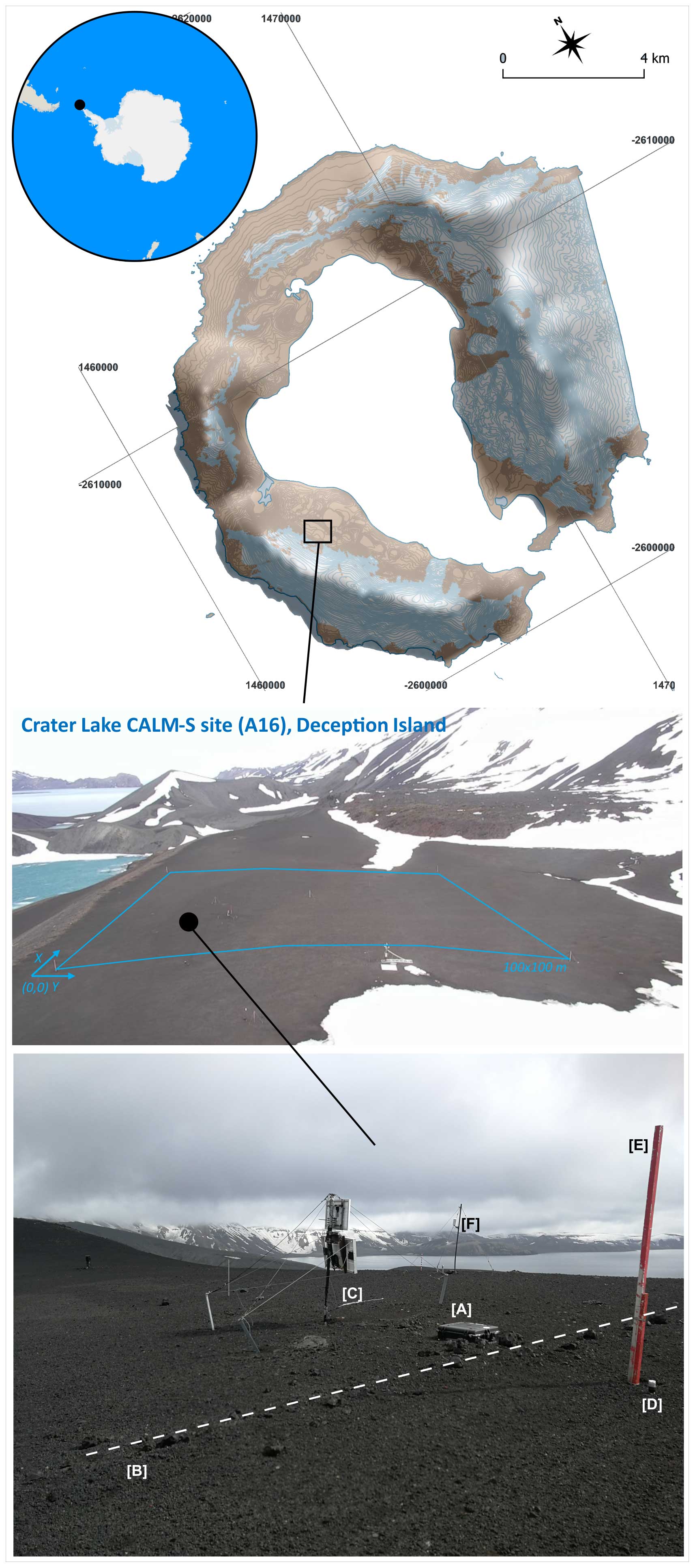
Figure 1 Location of the A-ERT setup at Crater Lake CALM-S site on Deception Island. The A-ERT box encasing the 4POINTLIGHT_10W resistivity meter instrument, solar-panel-driven battery, and multi-electrode connectors (A). Electrodes were buried in the ground and were connected to the cables (B). The solar panels are shown (C). Complementary environmental parameters are monitored close to the A-ERT profile at node x=30 m, y=30 m of the CALM's grid including borehole ground temperatures (D), snow thickness (E), and air temperature (F).

2.2 A-ERT monitoring setup

The A-ERT system, using a 4POINTLIGHT_10W (Lippmann) resistivity meter, originally deployed in 2010 (see Farzamian et al., 2020), was upgraded and reinstalled in February 2019 for long-term quasi-continuous monitoring along the same transect in the vicinity of the ground temperature borehole S_3,3. The upgrades compared to 2010 include the measurement of battery voltage and the temperature of the resistivity meter at the time of each ERT survey. These upgrades allow us to monitor the power demand of the system and the temperature fluctuations to which the resistivity meter is exposed. The hardware details of this A-ERT setup are very similar to those described in detail in Farzamian et al. (2024b) although our setup on Deception Island does not have the timer solution to switch off the system after each survey. The same survey parameters were used to collect A-ERT data in 2010 and 2019, enabling comparison of the two datasets. A-ERT surveys were performed using the Wenner electrode configuration for optimized energy consumption and higher vertical resolution to best differentiate the active-layer–permafrost boundary (Loke, 2002). A total of 20 electrodes with a spacing of 0.5 m were installed at the site, yielding 56 individual data points for each monitoring dataset at six data levels. The measurements started in February 2019 and were repeated every 6 h. The measurements were stored in the internal memory of the 4POINTLIGHT_10W device. This study focuses on A-ERT data collected from February 2019 to February 2020, offering a year-round dataset showcasing the A-ERT data variability and allowing for a comparison with the original A-ERT dataset from 2010. Mechanical probing before the A-ERT installation in 2019 and after data download in 2020 also allows for a comparison with ALT data derived from mechanical probing.

2.3 A-ERT data processing

ERT data can be susceptible to various sources of noise, such as poor galvanic contact, random errors, and polarization effects. In our setup, poor galvanic contact and the measurement of high resistivities at very low currents are considered to be the dominant sources of error. To improve the quality of the data and identify poor-quality measurements, we applied a minimum of five and a maximum of nine stacks per quadrupole, with a target standard deviation of 2 %. While stacking variance can be useful for identifying bad measurements, we observed that it is possible for outlier measurements to have low stacking errors. This suggests that relying solely on stacking error is ineffective for data processing, as has been discussed by other authors (e.g., Tso et al., 2017). Therefore, additional filtering is necessary to automatically identify and remove poor-quality data. Automated data filtering workflows are particularly valuable in our setup, where the large number of datasets per year makes manual data checking and filtering impractical.

Following the automated data filtering routine outlined by Herring et al. (2023), we implemented a series of filtering steps. Each filtering step required quantitative thresholds of data quality, which were determined empirically by iteratively testing the filtering algorithm on random subsets of the data and selecting thresholds that worked well for all datasets. In the first filtering step (step 1), we removed data points where the apparent resistivity was less than or equal to 0, data points with a stacking error greater than 2 %, and measurements with anomalously high apparent resistivity, defined as values greater than 9 times the standard deviation of the entire technically filtered dataset to account for different types of measurement error. This removal of physically unrealistic values is a reasonable data filtering step for any site. Next, in step 2, the moving median filter calculated a moving median of logarithmic apparent resistivities along each depth level in the pseudosection, using a window of five data points (except at the edges of the pseudosection, where a smaller window was necessary). Data points that deviated from the moving median by more than 7 % were removed. We also introduced a filtering step (step 3) that identified “bad” electrodes by evaluating how many data points associated with a particular electrode were removed in the previous steps. If more than 25 % of the data points measured by an electrode were removed, all the remaining data points from that electrode were discarded. Finally, in step 4, any datasets where more than 30 % of the data had been filtered in the previous steps were considered of poor quality and were not inverted, as the results would be too unreliable in a time-lapse modeling context.

2.4 ERT data inversion and analysis

Following the data filtering, all data were inverted using pyGIMLi, an open-source software package for geophysical modeling and inversion (Rücker et al., 2017). An L1 or “blocky” model norm was used due to its ability to better resolve sharp boundaries and large resistivity contrasts (Loke et al., 2003), like those expected between the thawed surface layer and the frozen ground beneath. Since the choice of regularization parameter controls the relative weighting of model and data misfit terms in the inversion, it is important to choose this parameter judiciously to avoid an overly smooth or noisy model. Here, the regularization parameter was optimized by an L-curve method using a built-in pyGIMLi function, a process which tests several regularization values and determines the optimal value (Günther et al., 2006). A simple linear noise model is typically used to estimate data error (Tso et al., 2017). Here, a noise model was created with 4 % relative noise and a small noise floor, taken to be 0.001. The starting model was set to a homogenous model of the average apparent resistivity for the first dataset in each monitoring period, while subsequent inversions used the previous inverted model (i.e., a “cascaded” inversion approach). The inversion proceeded until χ² was equal to 1 (i.e., the data were fit to within the assumed noise levels), a maximum number of iterations was reached (here set to 20 iterations), or the inversion converged (here taken to be when the objective function changed by less than 1 % between iterations).

After inversion, several analyses were conducted in order to extract the key information required for a detailed investigation of permafrost and active-layer dynamics. Similar to Farzamian et al. (2020), inverted resistivities were plotted for a virtual borehole in the center of the profile, close to the existing borehole S_3,3, enabling easy visualization of temporal patterns and comparison of inverted resistivities of A-ERT data from 2019 to 2010. This virtual borehole analysis is also used to compare the A-ERT results to the corresponding temporal borehole thermal variations obtained from S_3,3. In addition, the model coverage, which is calculated with a built-in pyGIMLi function by summing the entries of the Jacobian and normalizing by cell volume, was incorporated as an opacity filter in order to assess the reliability of the models.

To delineate the active layer and permafrost and to map the progression of thaw depth, we used the gradient method. This method is a reliable way to identify structurally simple unfrozen–frozen interfaces (Herring and Lewkowicz, 2022) based on their large resistivity contrast. At Crater Lake, the presence of an ice-rich top of permafrost layer improves this approach, since it results in a very high vertical resistivity contrast. Thaw depths were only interpreted when the near-surface resistivity was low (i.e., unfrozen). The results were then compared to the manual probing data and borehole temperatures. Furthermore, to facilitate assessment of temporal resistivity changes in the permafrost zone, a zone of interest was delineated at the center of the resistivity model from 2–7.5 m along the survey and 0.5–1.5 m depth. This zone of interest represents a well-resolved zone of the permafrost (i.e., beneath the permafrost table and in a region of higher sensitivity away from the edges of the model). Similar methodologies to examine resistivity in a zone of interest have been applied in previous studies (e.g., Etzelmüller et al., 2020; Kneisel et al., 2014; Mollaret et al., 2019).

3 Results

3.1 Analysis of observational data

Figure 2 shows mean monthly air temperatures and snow thickness at Crater Lake from 2010 to 2019, observed close to the middle of the A-ERT transect (see Fig. 1 for the locations of sensors and A-ERT profile), to present the general trends in temperatures and snow thickness in this period. Mean monthly air temperatures at Crater Lake from 2010 to 2019 showed a slight cooling until 2015 followed by a slight warming, with mean annual air temperatures ranging from −3.2 °C in 2015 to −0.8 °C in 2018. Mean monthly snow thickness followed a general trend similar to the air temperature, with years such as 2011 and 2019 showing shallow snow pack (<10 cm), while 2014, 2015, and 2016 showed longer and thicker snow cover (>20 cm). Overall, the data show that interannual conditions are variable both in snow cover and temperature and that 2010 and 2019 have comparable temperatures but different snow regimes.

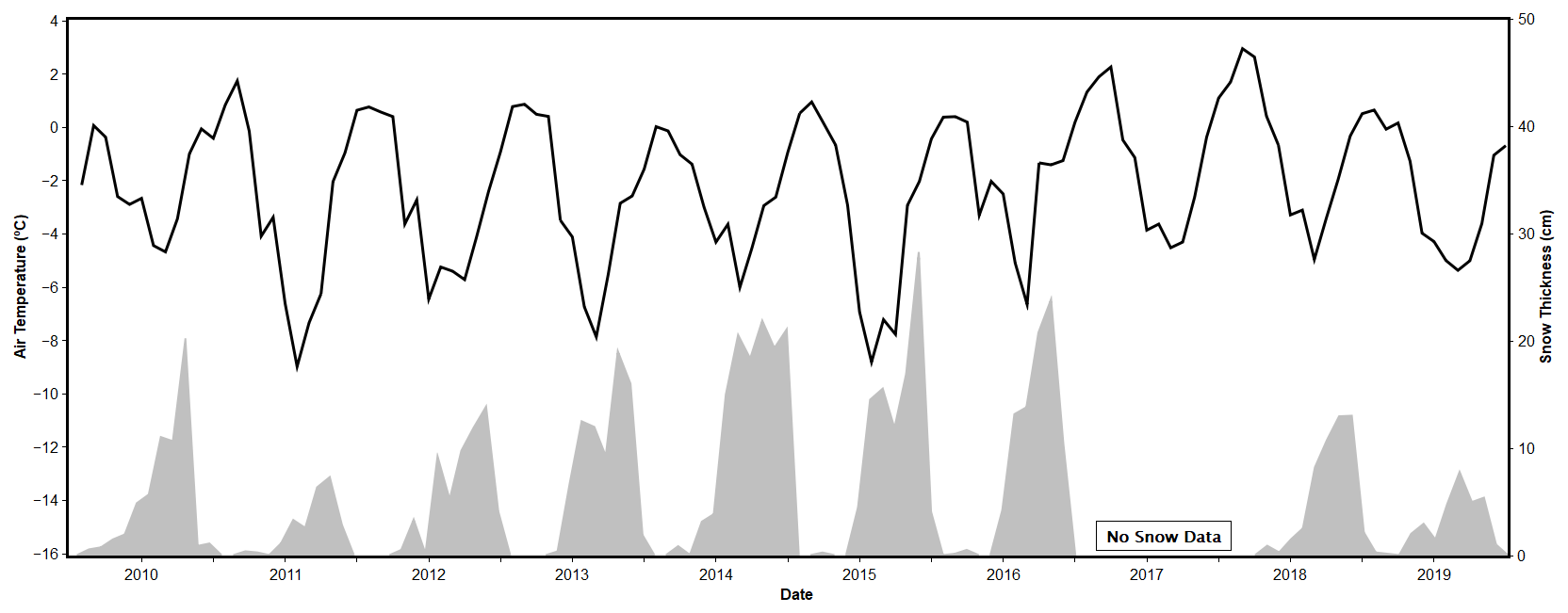
Figure 2 Mean monthly air temperatures and snow thickness at Crater Lake from 2010 to 2019, observed close to the middle of the A-ERT transect.

Figure 3 shows detailed variations in snow cover thickness, air, and borehole temperature during the A-ERT monitoring periods in 2010 and 2019. Snow cover during winter was generally thin, with only 5 to 30 cm thickness and frequent snow-free periods (Fig. 3a). The number of days with snow cover was lower in 2019 (85 d) compared to 2010 (118 d). In addition, the snow thickness was also thinner in general in 2019, and the difference became more evident during October, which showed either snow-free or very thin (i.e., less than 5 cm) snow cover in 2019. The air temperature fluctuation (Fig. 3b) is very similar in 2010 and 2019, ranging from −13.8 to 2.8 °C in 2010 and from −13.9 to 2.8 °C in 2019. The mean annual air average temperature is slightly lower in 2019 (−2.9 °C vs. −2.3 °C in 2010), and the standard deviation was also slightly higher in 2019 (3.4 °C vs. 3.2 °C in 2010), suggesting 2019 was a slightly colder year with slightly larger temperature fluctuations at this site. Air and shallow ground temperature are generally well-coupled when there is no snow cover and with a slight phase lag when snow is present.

The ground temperature at three depths (5, 20, and 80 cm) is shown in Fig. 3c–e for S_3,3. Temperature fluctuates significantly at shallower depths (i.e., within the active layer) during the year, with temperatures at 5 cm depth ranging from −7.5 to 2.1 and −8.6 to 3.1 °C in 2010 and 2019, respectively, and from −6 to 0.5 and −7.1 to 1 °C at 20 cm depth in 2010 and 2019, respectively, reflecting the snow cover variability and air temperature fluctuations. The average ground temperature at these depths was slightly colder (i.e., 0.1 °C) in 2019 compared to 2010. Active-layer freezing started in mid-April in 2010 and in mid-May in 2019, showing a delay of about 1 month between 2010 and 2019. Due to the thin snow cover during freezing and its late onset, as well as the lack of significant soil moisture, no zero-curtain effect is evident in either year. In contrast, there is a zero-curtain phase of almost 1 month during the thawing season starting from mid-October in both years. During both years and apart from seasonal freezing and thawing, brief and superficial changes of the ground temperature around 0 °C are very frequent. A more detailed discussion of these short-lived meteorological events is presented by Farzamian et al. (2020). Similar surficial refreezing events can be also identified in 2019 in April and May.

Temperature fluctuations at the deeper layers (i.e., 80 cm), just below the permafrost table, show smaller amplitudes ranging from −3.9 °C to close to 0 °C in both years (Fig. 3e). While the temperature range of the permafrost is similar between the 2 years, permafrost is slightly warmer during the first 9 months of the year in 2019 and then slightly colder during the last 3 months. These small differences can be attributed to air temperature and snow cover differences, such as the cold event in early October 2019 that penetrated deeper in the absence of snow cover, leading to slightly lower temperatures in the last 3 months of 2019.

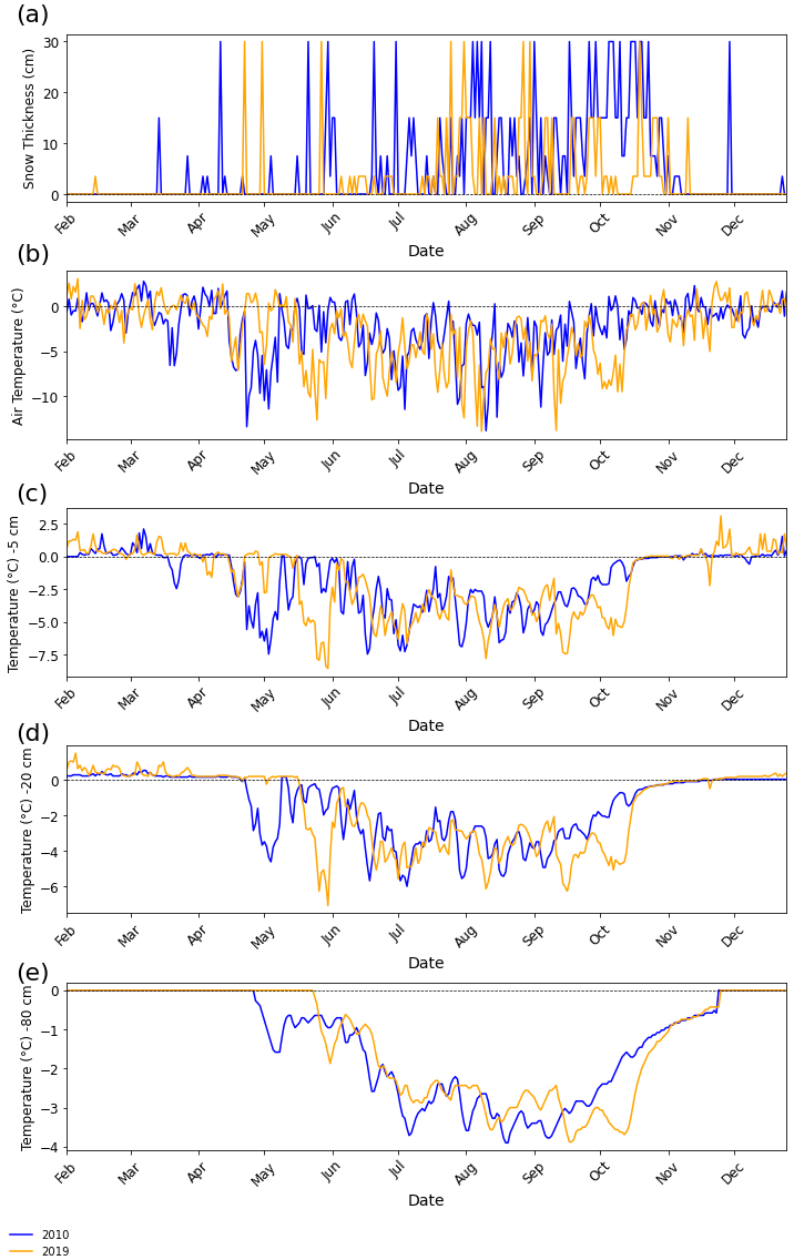
Figure 3 Comparative plots of 2010 and 2019: daily snow cover depth (a), air temperature (160 cm above the surface) (b), and ground temperatures at 5 cm (ground surface) (c), 20 cm (active layer) (d), and 80 cm (permafrost) depths (e).

3.2 Analysis of apparent resistivity data

Figure 4 shows an example of the application of a multi-step data processing workflow. Although the majority of datasets collected in 2010 and 2019 exhibit excellent quality, the presented example serves for illustrative purposes to demonstrate the functionality of the filtering scheme. Figure 4a represents the original data, while Fig. 4b–d display the filtered data after each step of the process. Through this multi-step data processing workflow, poor-quality measurements and anomalous data points were effectively eliminated, showcasing the effectiveness of the filtering procedure. This workflow was automated and applied to all datasets, enabling rapid and efficient identification and elimination of problematic data based on the same qualitative criteria. For other sites and applications, each step should be tested and threshold values adjusted as needed, as optimal values (specifically for steps 2–4) depend on the site conditions and data quality.

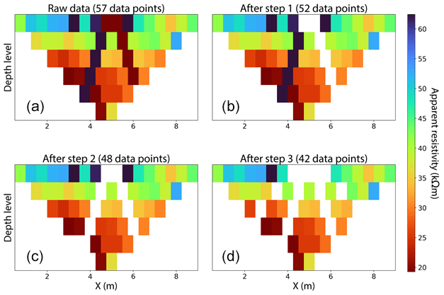
Figure 4 Multi-step data filtering to remove noisy data points: (a) field measurements; (b) data after application of filtering step 1 (removal of measurements that were ≤0, had poor repeatability, or were outliers relative to the rest of the dataset); (c) data after application of filtering step 1 and step 2 (moving median filter); and (d) data after the application of filtering step 1, step 2, and step 3 (bad electrode filter).

Overall, the A-ERT data in both years exhibited high quality, with less than 1 % of data points being removed by filtering and less than 0.5 % of A-ERT datasets being discarded due to poor quality (Fig. 5). Almost all of the discarded datasets were from the winter when the active layer is frozen and contact resistances at the electrodes are high (>100 kΩ). After processing and filtering the measurements, the mean daily apparent resistivity (ρ_a) values for each data level between 2010 and 2019 were plotted (Fig. 6).

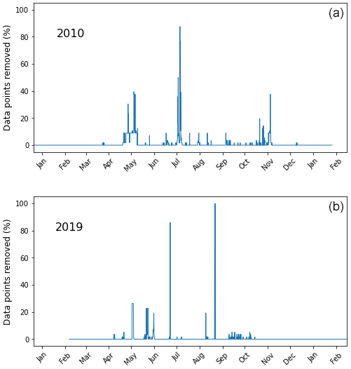
Figure 5 Data points removed using the automated data filtering routine for 2010 (a) and 2019 (b). Overall, less than 1 % of the data were removed.

In general, there is good agreement between the apparent resistivity data from 2010 (ρ_a2010) and 2019 (ρ_a2019), both during winter and summer. The shallow data, corresponding to electrode spacings of 0.5 and 1 m and investigation depths of ∼0.25 and 0.5 m, exhibit the highest temporal variability in both years, as these measurements are more influenced by significant resistivity changes during phase change processes (i.e., freeze and thaw events within the active layer), which are more frequent close to the ground surface. In mid-April, the ρ_a2010 data for 0.5 and 1 m electrode spacing experience a sharp rise in apparent resistivity within a 2-week period, starting from values below 20 kΩ m and exceeding 500 kΩ m by early May, indicating the onset of the seasonal freezing. ρ_a2019 data show a similar sharp rise in apparent resistivity in mid-May from values below 30 kΩ m to larger than 500 kΩ m in mid-May but within a shorter time interval (1 week). This suggests a 1-month delay in the seasonal freezing between 2010 and 2019 and agrees well with borehole information presented in Fig. 3c–e. The sharp increase in apparent resistivity in both years is attributed to the abrupt phase change upon freezing in the absence of a significant snow cover during April and May. Deeper levels, corresponding to electrode spacing of 1.5, 2, 2.5, and 3 m and investigation depths of ∼0.75–1.5 m, exhibit a delayed response, indicating the advancement of the freezing front, which aligns with the gradual decrease in the permafrost temperature with depth (see Fig. 3e).

Conversely, the beginning of the seasonal thawing phase in both years is characterized by a steady decrease in apparent resistivity, starting on 4 October and extending until the end of October in 2010 and starting on 15 October and continuing until mid-November in 2019. The gradual decrease in apparent resistivity during the thawing season, as opposed to the abrupt phase change in autumn, can be attributed to the presence of snow cover (Farzamian et al., 2020). The snow cover acts as an insulating layer, preventing the subsurface from being directly affected by warm-air signals in spring, thereby dampening the thawing process. Furthermore, the melting snow provides infiltrating water into the active layer close to 0 °C, which refreezes in contact with the colder ground (Scherler et al., 2010). During thawing, latent heat is absorbed and the temperature remains at 0 °C (zero-curtain effect). Similar to the temperature evolution, the deeper layers experience a delay in the resistivity decrease compared to shallower layers. Notably, this decrease in apparent resistivity was more gradual in 2010 compared to 2019, particularly at the beginning of the thawing season, where the resistivity decrease is sharper during 15–20 October compared to 2019. This is in good agreement with the temperature and snow cover data (Fig. 3).

Aside from the seasonal resistivity changes, the daily apparent resistivity fluctuations during 2010 and 2019 are generally small. However, there are notable fluctuations observed in both years, which are associated with brief surficial refreezing of near-surface layers during summer or short thawing periods in winter, as reported previously by Farzamian et al. (2020), resulting from short-lived meteorological extreme events with rapid and superficial changes in ground temperature around 0 °C.

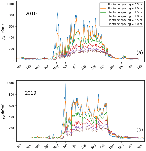
Figure 6 Apparent resistivity data of the A-ERT profile averaged for each electrode spacing for 2010 (a) and 2019 (b).

3.3 Analysis of inverted resistivity models

3.3.1 2D models

Figure 7 shows monthly modeled resistivity results for the years 2010 and 2019. The model coverage was plotted as an opacity filter to show where the model was more sensitive to the data (higher opacity) and less sensitive to the data (lower opacity). The data utilized in this analysis are from the 15th day of each month at 12:00 (in local solar time) for both years, showcased side by side for comparison. The RMSEs indicate that the inverted models are able to reproduce field data reasonably well. RMSEs for ERT data collected in permafrost environments usually range between 2 %–10 %, with higher values typically recorded in winter (Herring et al., 2023), which is in good agreement with the results from the Crater Lake A-ERT dataset.

The resistivity pattern observed along the A-ERT monitoring transect at the CALM-S site exhibits two distinct resistivity zones, and this distinction is evident in both years. The first zone, extending to a maximum depth of approximately 0.4 m during the summer months in both years, corresponds to the active layer, characterized by substantial resistivity changes during freezing and thawing events. The deeper zone captures the permafrost down to a depth of 2 m. The resistivity of both the active-layer and permafrost zones shows minimal lateral variation along this small transect, suggesting spatially homogeneous ground conditions in the study area. This observation aligns well with thaw depth measurements obtained using a mechanical probe, which also indicated limited spatial variability at this CALM site, particularly around the location of the A-ERT setup.

The top 40 cm, representing the active layer, undergoes the largest resistivity changes primarily during seasonal freezing and thawing events. In 2010, the most substantial resistivity changes commenced in May when the active layer froze. However, in 2019, the substantial resistivity changes associated with seasonal freezing are observed a month later in June, as already detected by borehole data (see Fig. 3c–e). Once the active layer freezes, heat is lost from deeper layers (i.e., permafrost zone), reducing unfrozen water content and consequently increasing resistivity in the winter months, as observed in both 2010 and 2019. While resistivity models in 2010 are generally similar to those in 2019 during winter, variations in resistivity values are also evident. For instance, modeling results in September and October show an overall more resistive subsurface in 2019 compared to the equivalent period in 2010, which can be attributed to cooler ground temperatures on 15 September and 15 October 2019, as seen in Fig. 3c–e.

The initiation of seasonal thawing is marked by a resistivity drop in November for both years. As the active layer thaws and heat flows into the permafrost zone, unfrozen water content increases and subsequently resistivity decreases are observed in December and January. An interesting episode that shows the relevance of A-ERT data for monitoring is the resistivity increase in the active layer in December 2010 following seasonal thawing. This indicates a brief surficial refreezing of the near-surface layer during this period, as also evident in the apparent resistivity data (Fig. 6). Shallow ground temperature data at 5 cm (see Fig. 3c) similarly recorded this brief freezing episode, occurring after subzero air temperatures during this period.

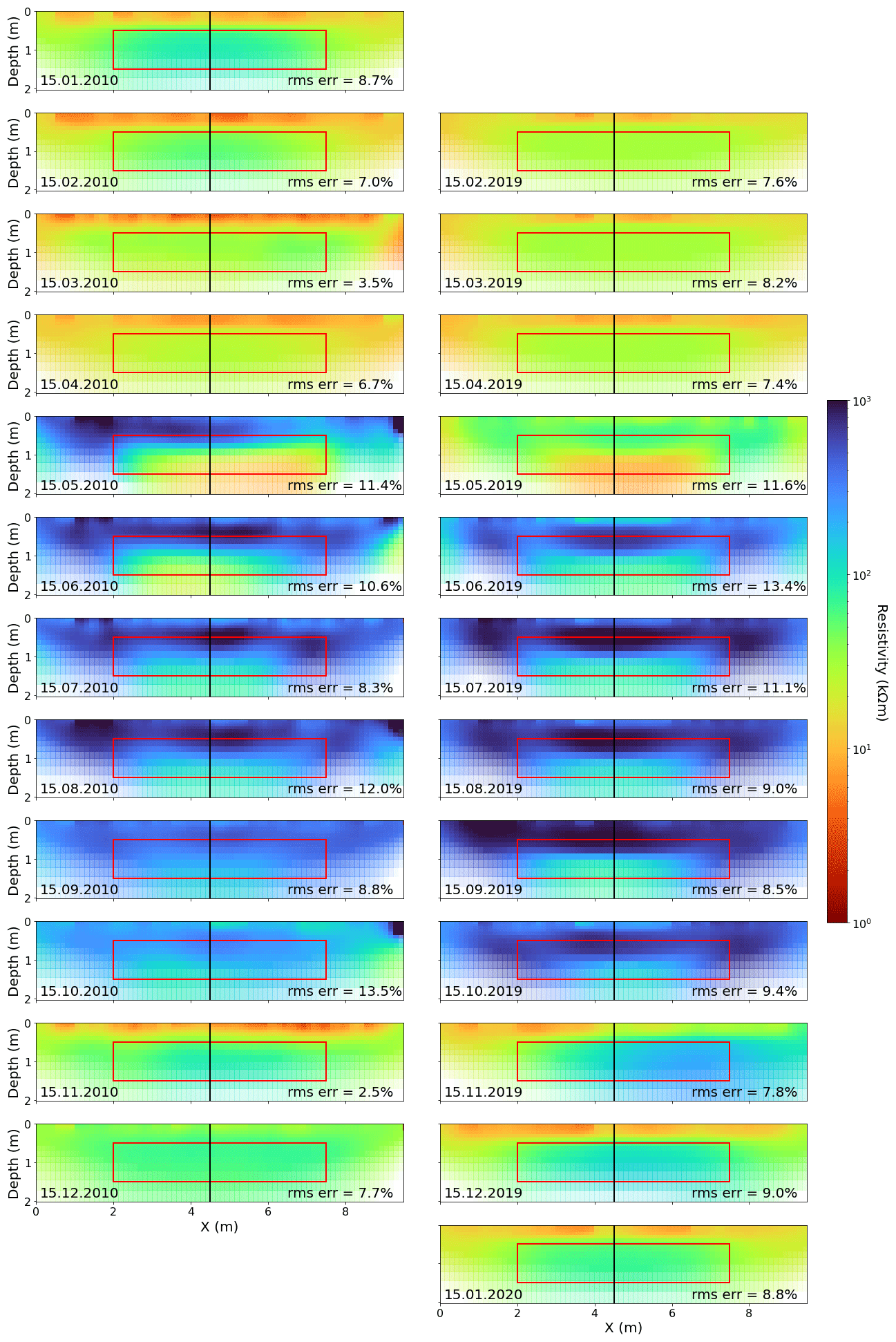
Figure 7 The 2D inverted resistivity models showing mid-month resistivity profiles for 2010 (left) and 2019 (right). The vertical black line denotes the position of the virtual borehole, and the red box denotes the zone of interest.

3.3.2 Virtual borehole

To better interpret temporal patterns in resistivity over time, resistivity values were extracted at a virtual borehole at the midpoint of the survey section. Figure 8 shows the evolution of inverted resistivity over time in the virtual borehole at the S_3,3 location during 2010 and 2019 (see Fig. 7 for the position of the virtual borehole). As in Fig. 7, the model coverage was plotted as an opacity filter to show where the model was more sensitive to the data (higher opacity) and less sensitive to the data (lower opacity). The resistivity values and model sensitivities varied depending on the season. In the summer, lower sensitivity at depth is due to preferential electrical current flow through the thawed active layer (e.g., Herring and Lewkowicz, 2022). Resistivity values in areas of the model with lower sensitivity should therefore be interpreted with caution.

There is good agreement between modeled results from 2010 and 2019 in terms of temporal and vertical resistivity values and their variability both during winter and summer. In both years, the highest resistivity values were observed in winter and near the permafrost table at depths around 0.40 m. This can be attributed to the cyclic process of water infiltration from snow or rain accumulating on top of the permafrost table, which undergoes repeated thawing and refreezing, forming an ice-rich layer (see for example Shur et al., 2005). The most drastic resistivity changes in the active layer occurred during the freezing phases in April 2010 and May 2019, with a 1-month lag between the 2 years. The active layer remained frozen until October in both years, except for a brief surficial thawing event between 7 and 14 May in 2010. Similarly, resistivity changes near the surface during winter coincided with consecutive cooling and warming of the active layer in both years (see Fig. 3).

Overall, the subsurface down to approximately 0.70 m exhibited lower resistivity values in 2010. This is likely due to slightly higher ground temperatures at shallower layers, as discussed in Sect. 3.1. The difference becomes more pronounced in May and June, with frequent warming events in 2010 that were absent in 2019. Increasing temperatures led to higher unfrozen water content and increased ion mobility, resulting in decreased resistivity. Interestingly, the slightly lower subsurface temperatures at greater depths (beyond 0.70 m) during October and November 2019 were reflected in the resistivity models, resulting in higher resistivity compared to the equivalent period in 2010.

The estimated active-layer depth using the maximum gradient method is shown as a red line in Fig. 8. The good agreement between the estimated depths and frost probe measurements (black dots) shows that maximum gradients are a reliable way to determine thaw layer depth and that A-ERT data can be used to infer real-time progression of thaw depth throughout the year. Based on these results, it can be concluded that the active layer at this site remains comparatively stable during the summer months in both years, with minor fluctuations ranging between ∼0.20 and 0.35 m.

The small temporal variability in thaw depth can be attributed to the presence of an ice-rich transient layer and permafrost table at this site and to the cool summers that characterize the maritime Antarctic, which do not significantly heat the soil. In January 2010, the average thaw depth was approximately 0.3 m, exhibiting a slight increase from late January until mid-March. These fluctuations correspond to higher air temperatures and subsequent active-layer warming, as evidenced by the shallow ground temperature measurements. The deepening of the active layer is followed by a rapid and brief freezing phase in mid-March, induced by subzero air temperatures. As the active layer cools and the infiltrating water above the permafrost table potentially refreezes, the active layer thins in late March and April, preceding the seasonal freezing. The thawing of the active layer initiates again at the beginning of November, with a relatively thinner thaw depth (around 0.2 m) at the start of the thawing season. However, the thaw depth gradually increases in late December as the active-layer warming extends to greater depths, influenced by warmer air signals during this period. The abrupt rise in resistivity observed in December coincides with the brief active-layer freezing occurring in that month. In 2019, the thaw depth is slightly thinner before the seasonal freezing (∼0.1 m compared to the equivalent period in 2010). In contrast to 2010, 2019 showed more frequent brief active-layer freezing events before seasonal freezing. This could account for a slightly thinner thaw depth in 2019 compared to the same period in 2010, as these events may lead to the freezing of unfrozen water atop the permafrost table, contributing to the shallowing of the active layer. In contrast, A-ERT did not detect any brief active-layer thawing event in 2019, unlike the occurrence in May 2010.

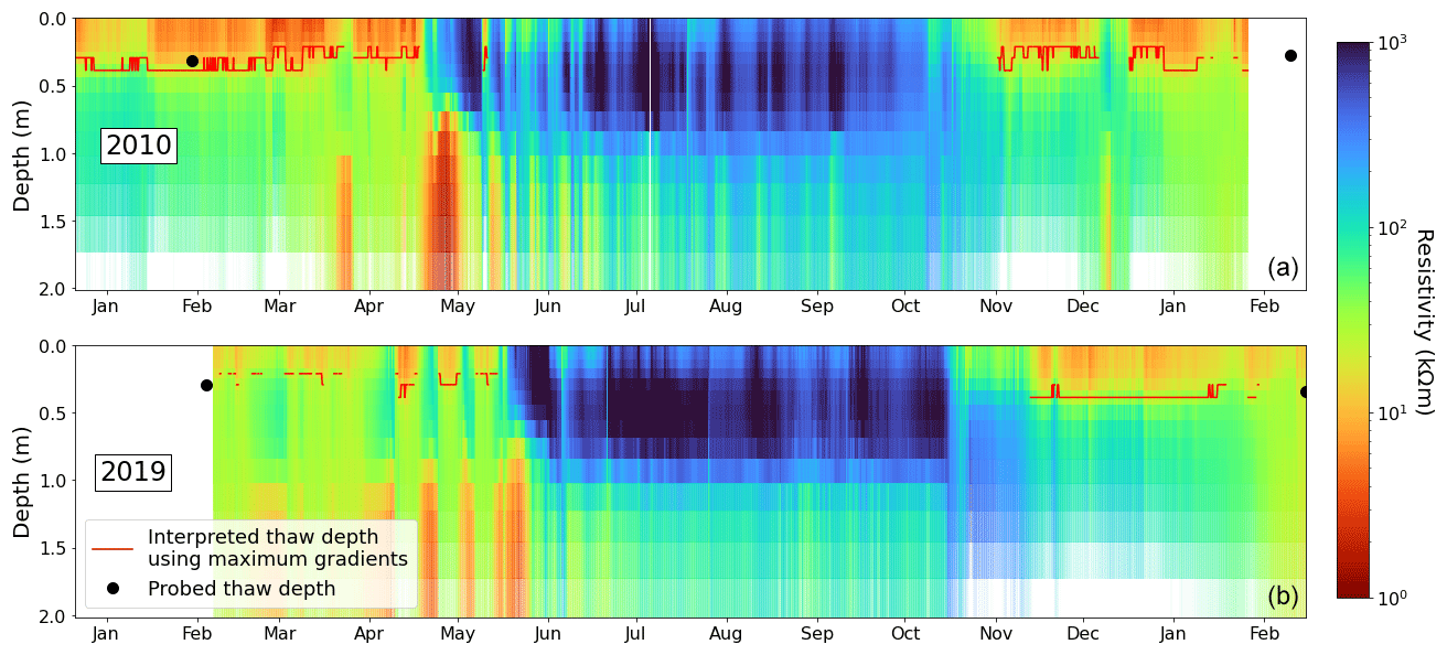
Figure 8 Inverted resistivities at a virtual borehole in the center of the ERT survey for 2010 (a) and 2019 (b) and interpreted thaw depth. Probed thaw depths are shown.

3.3.3 Average resistivity in zone of interest

To gain deeper insight into the resistivity changes within the permafrost zone and to examine the permafrost stability after almost a decade, daily resistivity and monthly average resistivity within the zone of interest ($\mathrm{2}<x<\mathrm{7.5}$ m and $\mathrm{0.5}<z<\mathrm{1.5}$ m; see Fig. 7) were calculated and are presented in Fig. 9. Box plot analysis was conducted on monthly data to depict the variability of resistivity within each month. The daily changes in resistivity within the zone of interest (Fig. 9a) align well with the ground temperature at a depth of 80 cm (permafrost zone; see Fig. 3e), indicating that resistivity variations follow permafrost temperature trends. Generally, there is good agreement between resistivities in 2010 and 2019 during the summer months and before seasonal freezing in April, as well as the winter period from June to September. During these periods, the resistivity difference is minimal, mirroring the small difference in ground temperature at 80 cm depth. A significant disparity in average resistivities occurs in May due to a phase change lag between 2010 and 2019, as seasonal freezing began about 1 month earlier in 2010 than it did in 2019. From October onward, the daily average resistivity tends to be higher in 2019 and remains elevated towards the end of the year. The most substantial difference is observed in October, aligning well with the ground temperature at 80 cm depth, where the temperature difference is most pronounced during this period. In the context of monthly resistivity changes, Fig. 9b also reveals that the monthly average resistivities in 2010 and 2019 are quite similar, except during seasonal freezing, influenced by a 1-month lag, and during the thawing season, influenced by slightly colder permafrost temperatures in late 2019. As anticipated, the most significant resistivity changes within each month and throughout the year occur during seasonal freezing and thawing events, driven by substantial subsurface resistivity changes during phase changes. The ongoing A-ERT monitoring will allow for the calculation of average resistivities at the yearly, seasonal, and monthly intervals, thus potentially providing new parameters that will enable the assessment of long-term permafrost changes. The analysis of parameter variability, such as the box plots in Fig. 9b, will enable the characterization of extreme melt or cooling events and the assessment of their impacts on the ground thermal regime.

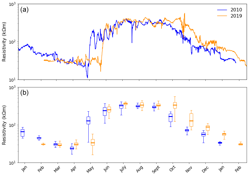
Figure 9 Average resistivity within the zone of interest ($\mathrm{2}<x<\mathrm{7.5}$ m and $\mathrm{0.5}<z<\mathrm{1.5}$ m) for (a) all datasets and (b) data grouped by month. The zone of interest is plotted in Fig. 7.

4 Discussion

The analysis of A-ERT data reveals predominantly good quality, with only a few problematic measurements observed during winter (Fig. 5) when subsurface freezing occurs and electrode contact may consequently be poor. However, the small number of bad measurements does not affect the real-time monitoring of subsurface resistivity and, consequently, thaw depth progression. The applied data processing technique enabled reliable spatiotemporal mapping of the subsurface, providing better insights on seasonal freezing and thawing as well as brief active-layer freezing and thawing events than would be obtained by borehole temperature monitoring alone. However, it is important to note that due to the homogeneity of the study site and the minimal variability of thaw depth along the A-ERT setup, significant lateral variability has not been observed in our modeling results. Additionally, the size of our A-ERT transect is relatively small compared to other A-ERT studies, where more pronounced lateral variations along the ERT transects are typically observed (e.g., Hilbich et al., 2011; Supper et al., 2014; Keuschnig et al., 2017). A-ERT monitoring, particularly using longer profile lengths, is expected to be even more advantageous at heterogeneous sites where point-location monitoring cannot capture lateral variability.

The depth of the maximum resistivity gradient correlated well with probed thaw depth, demonstrating that A-ERT can be used to accurately determine thaw depths over time. It is important to note that the resolution of thaw depth using this method depends on the acquisition parameters (e.g., electrode spacing and array type) that govern the resolution capabilities of the survey and also how finely the model is discretized. In this case, the cell heights in the top 0.4 m of the model were between 5–7 cm, with smaller cell sizes near the ground surface and gradually larger cells towards the base of the model.

The consistent patterns of resistivity changes observed during the seasonal freezing and thawing events in both years indicate that the sharp and rapid rise in resistivity (active-layer freezing) during winter, followed by a gradual and smoother resistivity change over a longer period of time (active-layer thawing), is likely typical for this site. These patterns can be attributed to the dynamics of snow cover and ground moisture, which were well-resolved by A-ERT in both observation periods. The A-ERT modeling results also reveal a consistently stable active layer at this site throughout the summer months in both years, with slight fluctuations within the range of approximately 0.20 to 0.35 m. However, the active layer appears slightly thinner and more resistive in early 2019. This can be attributed to slightly colder air and surface temperatures in early 2019, along with the impact of frequent brief freezing of the active layer before seasonal freezing in 2019, as detected by A-ERT. The ability of the A-ERT system to capture these rapid changes in the active layer, as a result of short-lived meteorological extreme events (see Farzamian et al., 2020), reaffirms the significance of the automatic ERT monitoring system in recording continuous resistivity changes.

The A-ERT setup provided valuable insights into the permafrost condition and evolution of ground ice at this site. Our detailed analysis indicates that there is no significant change in permafrost (e.g., ice degradation) after almost a decade. As shown, most of the differences in resistivity between 2010 and 2019 can be attributed to seasonal temperature variations and a phase change lag between these years. These findings align with the non-statistical insignificant warming trend in mean annual near-surface temperatures in the South Shetlands (0.028 °C yr⁻¹) from 2006 to 2020, as reported by Hrbáček et al. (2023) and from climate data obtained from this site (see Fig. 2). We anticipate that the site-specific conditions of our study site, characterized by an ice-rich permafrost table (confirmed by A-ERT data and cores), contributed to the stability of permafrost against potential degradation. In order to more accurately assess ice content at A-ERT monitoring sites, future work could incorporate additional complementary geophysical surveys, such as seismic surveys, which can significantly enhance our ability to quantify ice content. For example, seismic travel times can be used in a four-phase model (Hauck et al., 2008, 2011) to quantify water, air, and ice contents for a given porosity model. The joint application of ERT and seismic reflection data, combined with petrophysical joint inversion approaches (Wagner et al., 2019; Mollaret et al., 2020), has enabled quantitative estimates of water, air, ice, and rock volumes. These techniques could further improve ice content quantification and monitoring of its temporal evolution.

Compared to current traditional approaches such as boreholes and mechanical probing, A-ERT offers several practical advantages. Boreholes only provide limited 1D depth profiles at specific locations, which is insufficient to capture the variability observed in a spatial context. In addition, and in our case, the thaw depth variability in the 0.2–0.35 m range, seen in the resistivity data plotted at a virtual borehole, cannot be reflected in the ground temperature borehole data due to the lack of sensors in these depths. Furthermore, borehole data cannot offer the insights into the spatial and temporal variability of ground ice needed to evaluate permafrost stability. On the other hand, while mechanical probing can be used to determine the spatial variability of thaw depth over larger areas, it becomes impractical in many Antarctic regions with coarse and bouldery sediments or thick active layers. Moreover, logistical challenges and adverse weather conditions can impede manual probing at consistent time intervals, leading to biased information regarding thaw depth dynamics. These same logistical and weather challenges also apply to manually repeating ERT measurements, as reported by Etzelmüller et al. (2020), making the A-ERT method also advantageous over traditional manual ERT monitoring.

The high-resolution quantitative data from electrical resistivity measurements offer objective insights into changes in ground conditions, influenced by both climate conditions and geothermal heat fluxes. These data reveal variations in thermal state, ice content, and moisture, with the capability of monitoring at short and long time intervals. Given that the Global Climate Observing System defines ECVs as those physical, chemical, or biological variables (or groups of linked variables) that critically contribute to the characterization of Earth's climate (Bojinski et al., 2014), we propose that electrical resistivity has the potential to become a new ECV. This designation would promote its broader application and provide valuable data for understanding permafrost dynamics. Unlike the 1D nature of borehole temperatures, electrical resistivity methods can be used to characterize 2D transects or 3D volumes, enabling the observation of both vertical and lateral permafrost changes, thus bridging the gap between remote sensing observations and point data.

5 Conclusion and outlook

Geophysical techniques, especially ERT measurements, have become increasingly common in permafrost science to study active-layer and permafrost dynamics. Low-cost and low-power monitoring resistivity systems, such as the A-ERT system presented in this study, offer a unique means to investigate detailed freezing and thawing processes in permafrost regions in remote areas. This system can be operated with high temporal frequency, enabling the study of short-term meteorological events on permafrost and active-layer dynamics, as well as consistent analysis of long-term changes. Our detailed investigation of the A-ERT data and inversion modeling results shows that the A-ERT system detected the seasonal and brief surficial active-layer freezing and thawing events, as well as the phase change lag of almost 1 month between 2010 and 2019 during seasonal freezing. Without automated ERT monitoring, an identification of these events and the real-time progression of the thaw depth would not be possible. With the continuation of A-ERT measurements for long-term monitoring at Crater Lake, as well as at other sites in Antarctica (we have recently installed A-ERT systems on Livingston, King George, and James Ross islands), future calculations of monthly and even yearly resistivity changes within the permafrost zone can be conducted to assess permafrost stability. We propose that electrical resistivity could be used as a new essential climate variable for evaluating long-term permafrost changes, and it would be a valuable complement to other climate and borehole data.

Processing large-resistivity time-series data in such harsh environments needs to be carefully executed before any interpretation. The processing tool presented in this work, supported by the companion Jupyter Notebook, forms the basis for a semi-autonomous high-throughput processing workflow for dense temporal datasets collected by A-ERT systems. The implemented filtering tool processes all A-ERT data consistently using the same criteria, identifying and removing bad measurements, ensuring efficient handling of a large number of A-ERT data, and facilitating the prompt extraction of key information. The inversion process was then carried out using the open-source pyGIMLi library, and further processing was performed afterward to extract key information from a large amount of A-ERT data efficiently and quickly to study the active-layer and permafrost dynamics. For example, inverted resistivity plots at a virtual borehole enabled an efficient assessment of changing site conditions over short and long timescales and allowed for comparison to measured temperatures and manual probing. The gradient method applied in this study was an efficient way to delineate the interface between the thawed surface layer and underlying frozen ground. Calculating resistivity averages over a zone of interest (i.e., permafrost zone) also enhanced the assessment of permafrost conditions after almost a decade. Future work could incorporate additional information, like borehole temperatures, probed thaw depths, or other geophysical data, to constrain the inversion and increase model reliability. Furthermore, co-located seismic datasets could be used to quantify subsurface ice content.

Antarctic ice-free regions are facing rapid changes, forced by changes in solar radiation, temperature, snow, and rainfall events. Consequently, alterations of the active layer and permafrost are expected, potentially generating a cascade of effects mainly associated with surface and subsurface hydrology and geomorphic dynamics. These changes have the potential to impact terrestrial ecosystems, infrastructure, and nearshore and lacustrine environments. In this context, future installations of A-ERT monitoring systems will contribute to gaining deeper insights into permafrost and active-layer dynamics in Antarctica and permafrost regions globally.