Modelling subglacial fluvial sediment transport with a graph-based model, Graphical Subglacial Sediment Transport (GraphSSeT)

A quantitative understanding of how sediment discharge from subglacial fluvial systems varies in response to glaciohydrological conditions is essential for understanding marine systems around Greenland and Antarctica and for interpreting sedimentary records of cryosphere evolution. Here we develop a graph-based approach, Graphical Subglacial Sediment Transport (GraphSSeT), to model subglacial fluvial sedimentary transport using subglacial hydrology model outputs as forcing. GraphSSeT includes glacial erosion of bedrock and a dynamic sediment model with exchange between the active transport system and a basal sediment layer. Sediment transport considers transport-limited and supply-limited regimes and includes stochastically evolving grain size, network-scale flow management, and tracking of detrital provenance. GraphSSeT satisfies volume balance and sediment velocity and transport capacity constraints on flow. GraphSSeT is demonstrated for synthetic scenarios that probe the impact of variations in hydrological, geological, and glaciological characteristics on sediment transport over multi-diurnal to seasonal time frames. For steady-state hydrology scenarios on seasonal timescales, we find a primary control from the scale and organisation of the channelised hydrological flow network. The development of grain-size-dependent selective transport is identified as the major secondary control. Non-steady-state hydrology is tested on multi-diurnal timescales for which sediment discharge scales with peak water input, leading to increased sediment discharge compared to the steady state. Subglacial hydrology models are being applied more broadly, and GraphSSeT extends this capacity to quantitatively define the volume, grain-size distribution, and detrital characteristics of sediment discharge that through comparison with the sediment record may enable improved knowledge of the glaciohydrological system and its impact on marine systems.

1 Introduction

Discharge of sediments from subglacial fluvial systems is an important component of the ocean system and impacts the delivery of nutrients (Wadham et al., 2013; Meire et al., 2017; Cape et al., 2019; Overeem et al., 2017), ice-shelf cavity processes (Smith et al., 2019), and marine geomorphology (Dowdeswell et al., 2016, 2015). Turbid sediment plumes provide a means to observe subglacial fluvial inputs into the ocean that are difficult to observe in situ (Schild et al., 2017; Chu et al., 2009). Furthermore, marine sediments from currently or formerly glaciated margins are a primary record of past cryosphere change and are crucial to develop knowledge of global climate evolution (Lepp et al., 2022; Hogan et al., 2020, 2011; Witus et al., 2014; Hogan et al., 2012; Andresen et al., 2024).

In sub-ice sheet settings, subglacial fluvial systems comprise a multi-scale system with flow varying on timescales spanning hours to centuries or more. Of particular interest are events of short duration but with high flow (Dow, 2022; Dow et al., 2022; Chu, 2014; Ashmore and Bingham, 2014), associated with seasonal to diurnal surface melting cycles (Ehrenfeucht et al., 2023) and flood events, including jökulhlaups (Roberts, 2005). Ice stream water piracy involving the re-routing of subglacial water from one ice stream to another may rapidly reorganise the drainage regime, even with small changes in glacial mass balance or bed conditions (McCormack et al., 2023; Alley et al., 1994; Vaughan et al., 2008). It is likely that ongoing changes in cryosphere systems will increase the frequency and intensity of high-flow events in the future and so increase sediment flux to the ocean (Delaney and Adhikari, 2020)

To implement the consequences of cryosphere change on marine systems and to fully comprehend the implications of sedimentary records of the past and present cryosphere, a quantitative understanding of subglacial fluvial sediment transport systems is needed (Delaney and Adhikari, 2020). Here we describe a new graph-based approach to modelling subglacial fluvial sediment transport, Graphical Subglacial Sediment Transport (GraphSSeT). The approach is demonstrated for glaciohydrological scenarios across a range of time- and length-scales using subglacial hydrology model outputs (De Fleurian et al., 2018). We assess the most important hydrological, geological, and glaciological controls on the sediment transport system.

2 Background

GraphSSeT seeks to provide a versatile environment for modelling subglacial sediment transport, including the efficient delineation of channelised hydrology networks, a dynamic sediment model (Delaney et al., 2019), and network-scale flow management. GraphSSeT outputs the key information used to constrain sedimentary systems, including the volume, concentration, and grain-size distribution of sediment and its detrital characteristics. The model is stochastic and is particularly well-suited to developing a representative understanding of the sediment transport system for specific glaciohydrological scenarios.

2.1 Conceptual background

2.1.1 Subglacial hydrology

Under ice, water transport occurs in response to hydraulic potential gradients that drive flow towards lower-potential areas (Shreve, 1972). The subglacial hydrology system comprises input, storage, flow, and output (Ashmore and Bingham, 2014). Water enters the subglacial hydrology flow network by the melting of basal ice, groundwater discharge, subglacial lake discharge, and surface melt transported to the bed through moulins. In the context of the modelling to come, we make a distinction between distributed inputs occurring over a substantial area, e.g. from basal melt, and focused inputs with a high-volume input at specific locations, e.g. from surface water input via moulins. Water may be stored englacially (Fountain et al., 2005) and in subglacial lakes, which may be active lakes that fill and empty in a cyclical to episodic fashion or stable lakes (Livingstone et al., 2022). Water may also be stored in sediments and sedimentary rocks (Christoffersen et al., 2010; Flowers and Clarke, 2002).

Subglacial water flow may be characterised by a distributed, or so-called sheet flow, along the bed interface, which is relatively inefficient, or characterised by flow concentrated into subglacial channels, so-called channelised flow, which is relatively efficient. Distributed flow may be accommodated by several mechanisms including linked-cavity systems (Kamb, 1987), distributed canals eroded into underlying sediment (Walder and Fowler, 1994), thin patchy films (Alley, 1989; Creyts and Schoof, 2009), or flow through permeable basal sediments (Boulton et al., 2007); more generally, the bed may be viewed as a permeable interface (Hewitt, 2011; Flowers et al., 2004). Channels may be incised into the overlying ice, forming so-called Röthlisberger or R channels (Röthlisberger, 1972) that evolve dynamically in response to water and ice flow. Classical R channels are semi-circular in section (Röthlisberger, 1972) but may be more generally viewed as circle segments with a geometry defined by the so-called Hooke angle, allowing for broad, low conduits (Hooke et al., 1990). Alternatively, channels may form by incision into the bed, forming so-called Nye or N channels (Nye, 1976). Outputs from the subglacial hydrology system include discharge to the ocean, re-freezing to the bed (Alley et al., 1998), filling of lakes and englacial reservoirs, or recharge of groundwater aquifers.

The hydrology system is strongly influenced by quasi-stable basal boundary conditions, including bed topography, bed roughness, subglacial geology, and geothermal heat flux, and is intrinsically linked to ice dynamics, including changes in ice thickness and surface slope as well as the thermal state and flow dynamics of the ice. Particularly important are the temporal and spatial variations in hydrological inputs that may occur over timescales from hours to millennia.

2.1.2 Subglacial sediment transport

Glaciers can transport sediment entrained within the basal ice (Licht and Hemming, 2017) and through basal sliding, causing sediment to move with the ice (Evans et al., 2006; Christoffersen et al., 2010). These transport processes have previously been represented in ice sheet models (Pollard and DeConto, 2020) and are not the focus here. Subglacial fluvial transport is the other major component of sediment discharge (Overeem et al., 2017; Andresen et al., 2024) and is more sensitive to changes in the glaciohydrological state. This highly dynamic spatiotemporal transport system is the focus of our model. Important considerations include the dual limits on transport from transport capacity and sediment supply and the interaction of changing hydrology with an evolving basal interface.

The dynamics of subglacial fluvial sediment transport are not well constrained by observations. However, they share similarities with fluvial transport in rivers for which the governing processes are better-established (van Rijn, 2007a, b; Ancey, 2020a, b). The physical description of fluvial transport processes is often uncertain with respect to satisfying empirical data, but several classes of transport law are well-established. One major family of such laws uses the shear stress at the bed to establish transport capacity, using either stochastic or deterministic criteria for sediment mobilisation (Engelund and Hansen, 1967; Meyer-Peter and Müller, 1948; Einstein, 1950). These laws have been applied to develop the first dedicated model for subglacial fluvial sediment transport – the SUbGlacial SEdiment Transport (SUGSET) model – with formulations in one dimension (Delaney et al., 2019) and recently in two dimensions (Delaney et al., 2023). Network-based models are developed for riverine fluvial systems (Czuba, 2018; Wilkinson et al., 2006) but no network-based formulation exists for subglacial fluvial systems.

2.2 Modelling background

2.2.1 Subglacial hydrology models

Subglacial hydrology may be described by models with varying degrees of complexity (Flowers, 2015). The simplest models use the so-called Shreve potential (Shreve, 1972) to define the direction and relative magnitude of water flow (Eq. 1).

$$\begin{array}{}\text{(1)}& \mathit{\phi }={\mathit{\rho }}_{\mathrm{i}}g{z}_{\mathrm{s}}+({\mathit{\rho }}_{\mathrm{w}}-{\mathit{\rho }}_{\mathrm{i}})g{z}_{\mathrm{b}}+N,\end{array}$$

where φ is the hydraulic potential at the bed for an ice surface elevation z_s and bed elevation z_b. ρ_i and ρ_w are the densities of ice and water respectively and g is gravitational acceleration. N is effective pressure, defined as ice overburden pressure minus the basal water pressure. Assuming constant N, the hydraulic potential gradient may be defined as

$$\begin{array}{}\text{(2)}& \mathrm{\nabla }\mathit{\phi }={\mathit{\rho }}_{\mathrm{i}}g\mathrm{\nabla }{z}_{\mathrm{s}}+({\mathit{\rho }}_{\mathrm{w}}-{\mathit{\rho }}_{\mathrm{i}})g\mathrm{\nabla }{z}_{\mathrm{b}}.\end{array}$$

With water input applied to the bed, flow can be accumulated to define regions of enhanced flow (Le Brocq et al., 2009). Shreve potential approaches have the benefit of low computational cost, simplicity, and ease of application. However, with the assumption of constant N, they do not represent the dynamic interactions of distributed and channelised flow well on short timescales or on the length scales of individual channels (De Fleurian et al., 2018).

More-advanced formulations include a network-based approach that considers flow to represent both channels and linked cavities in a unified form as conduits (Schoof, 2010) and approaches that involve a coupled model of channelised and distributed flow regimes, considering the development of each and the transfer of water between them (Flowers et al., 2004; Hewitt, 2011). For GraphSSeT (Fig. 1), any model for which channelised flow can be described on a set of connected edges could be used as input, but the one used as forcing here is the Glacier Drainage System (GlaDS) model based on the finite-element method (FEM) (Werder et al., 2013).

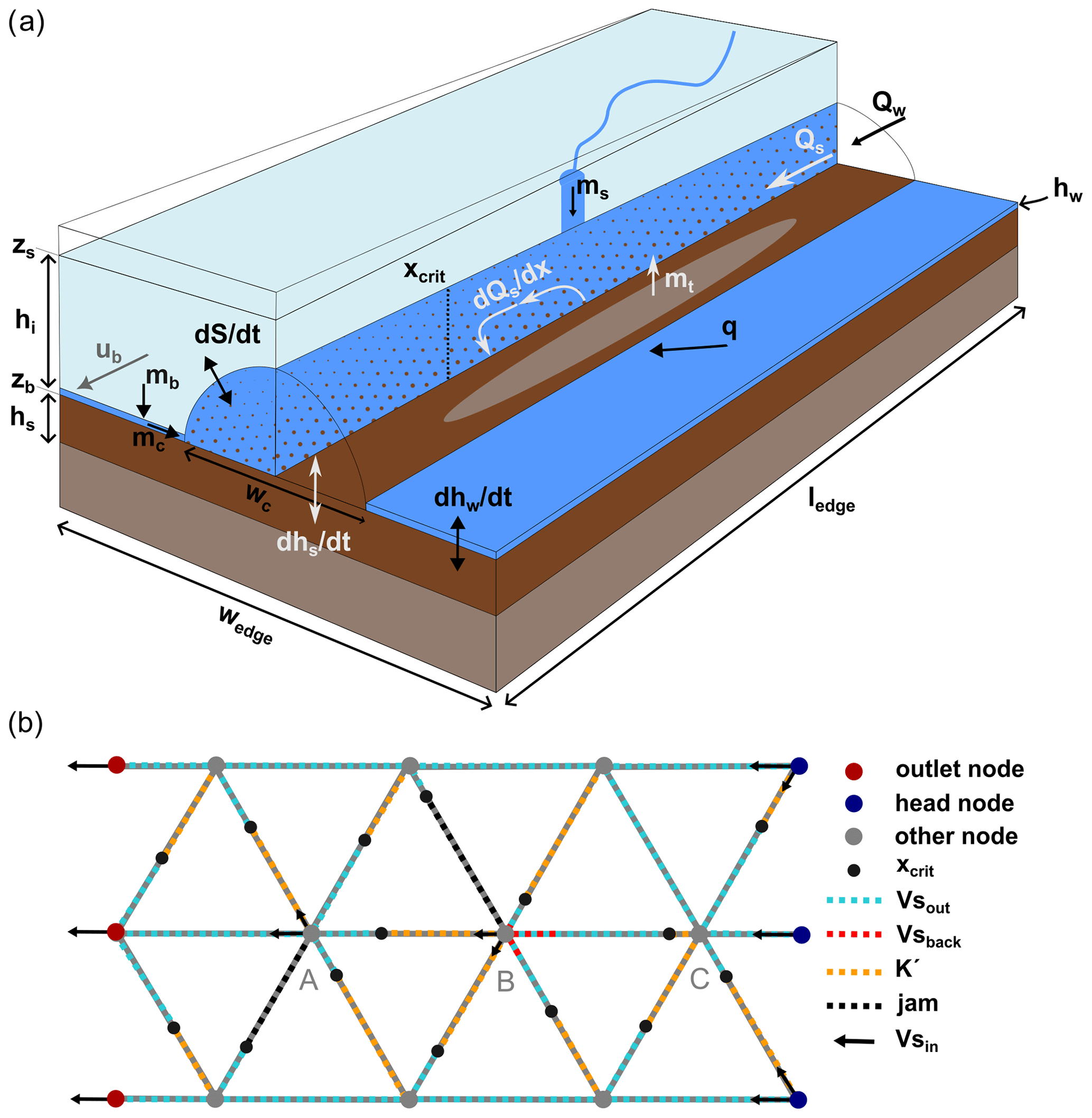
Figure 1 (a) Schematic of a GraphSSeT model edge showing its structure and key model components. Hydrology model components are in black, ice sheet model components are in grey, and sediment model components are in white. Variables and quantities for GlaDS and SUGSET are as in Sect. 2.2.2 and 2.2.3 respectively. (b) Schematic illustrating the network transport model (see Sect. 2.2.4). This example shows three interconnected channels, each with flow from the head node to the outlet node. The northern and southern channels have supply-limited conditions, where all sediment is able to leave the edge ($V_{s_{\mathrm{out}}}$ is sediment leaving the edge). The central channel and connecting edges have transport-capacity-limited conditions, and sediment will only leave the edge from below the critical point x_crit. Furthermore, the edges downstream of node B cannot transport the sediment supplied from upstream. The consequence is that residual sediment volume (as flux density, K^′) accumulates on the downstream edges, and there is ultimately reduced flow ($V_{s_{\mathrm{in}}}$) into the downstream edges, balanced by backflow ($V_{s_{\mathrm{back}}}$) on the upstream edges: excessive flux density causes an edge to jam. Jammed edges cannot receive incoming sediment volume, but sediment can flow out to the downstream edges, allowing the jam to clear.

2.2.2 The GlaDS model

For sheet flow, we begin with the conservation of mass,

$$\begin{array}{}\text{(3)}& {\displaystyle \frac{\partial h_{\mathrm{w}}}{\partial t}}+\mathrm{\nabla }\cdot \mathit{q}=m_{\mathrm{b}},\end{array}$$

where h_w represents the water sheet thickness, and m_b describes water input to the sheet. q is the sheet discharge and is defined as a Darcy–Weisbach turbulent flow parameterisation $\mathit{q}=-k{h}_{\mathrm{w}}^{\mathit{\alpha }}|\mathrm{\nabla }\mathit{\phi }{|}^{\mathit{\beta }-\mathrm{2}}\mathrm{\nabla }\mathit{\phi }$, where k, α, and β are defined appropriately for the flow law (Werder et al., 2013). The evolution of the sheet thickness is modelled on elements and is formulated using a linked cavity approach (Hewitt, 2011),

$$\begin{array}{}\text{(4)}& {\displaystyle \frac{\partial h_{\mathrm{w}}}{\partial t}}=\mathit{\omega }-\mathit{\upsilon },\end{array}$$

where ω represents the cavity opening rate as

$$\begin{array}{}\text{(5)}& \mathit{\omega }\left(h_{\mathrm{w}}\right)=\left\{\begin{array}{ll}{u}_{\mathrm{b}}(h_r-h_{\mathrm{w}})/l_r& \text{if }{h}_{\mathrm{w}}<h_r\\ \mathrm{0}& \text{otherwise},\end{array}\right.\end{array}$$

with u_b representing the basal sliding velocity of ice, and h_r and l_r are the typical bedrock bump height and horizontal cavity spacing respectively. In Eq. (4), υ represents the cavity closing rate as

$$\begin{array}{}\text{(6)}& \mathit{\upsilon }(h_{\mathrm{w}},N)=\stackrel{\mathrm{̃}}{A}{h}_{\mathrm{w}}|N{|}^{\mathit{\eta }-\mathrm{1}}N,\end{array}$$

where $\stackrel{\mathrm{̃}}{A}$ is the ice flow constant scaled for cavities, and η is the Glen's flow law exponent, typically 3.

Channelised flow is modelled on element edges, with each edge representing a potential channel that can open and close according to the balance between ice creep and melting of the channel walls. Again, we begin with the conservation of mass,

$$\begin{array}{}\text{(7)}& {\displaystyle \frac{\partial S}{\partial t}}+{\displaystyle \frac{\partial Q_{\mathrm{w}}}{\partial x}}={\displaystyle \frac{\mathrm{\Xi }-\mathrm{\Pi }}{{\mathit{\rho }}_{\mathrm{w}}L}}+m_{\mathrm{c}},\end{array}$$

where x is the coordinate along the edge, Ξ is the potential energy dissipated per unit length and time, and Π is the sensible heat exchange of water due to melting or refreezing (see Werder et al., 2013, for definitions of Ξ and Π). L is the latent heat of fusion. Q_w is defined as a Darcy–Weisbach turbulent flow parameterisation $Q_{\mathrm{w}}=-k_{\mathrm{c}}{S}^{{\mathit{\alpha }}_{\mathrm{c}}}|\frac{\partial \mathit{\phi }}{\partial x}{|}^{{\mathit{\beta }}_{\mathrm{c}}-\mathrm{2}}\frac{\partial \mathit{\phi }}{\partial x}$, with k_c, α_c, and β_c not necessarily representing the same values as those for sheet flow. m_c is the water entering the channel from the adjacent sheet. The time evolution of channel area S is given by the balance of the opening rate and closing rate,

$$\begin{array}{}\text{(8)}& {\displaystyle \frac{\partial S}{\partial t}}={\displaystyle \frac{\mathrm{\Xi }-\mathrm{\Pi }}{{\mathit{\rho }}_{\mathrm{i}}L}}-{\mathit{\upsilon }}_{\mathrm{c}}.\end{array}$$

The closing rate υ_c is defined similarly to Eq. (6), replacing h_w with S and with potentially different scaling for $\stackrel{\mathrm{̃}}{A}$.

The sheet and the channel model are coupled by requiring that the pressure is continuous; i.e. the pressure in the sheet and in an adjacent channel is equal. The continuity is assured by fixing the water exchange between the sheet and the channels accordingly (via m_c for the channels and via boundary conditions for the sheet).

2.2.3 Subglacial sediment dynamics model

For sediment transport in GraphSSeT, we discretise the one-dimensional form of the SUGSET model (Delaney et al., 2019) to apply to graph edges (Fig. 1). The channel dimensions and flux may be calculated from water inputs or may be obtained a priori from an input hydrology model, which is the approach we use here. With knowledge of the channel sectional area and channelised water flux, the basal shear stress from water flow is

$$\begin{array}{}\text{(9)}& \mathit{\tau }={\displaystyle \frac{\mathrm{1}}{\mathrm{8}}}{f}_r{\mathit{\rho }}_{\mathrm{w}}{u}_{\mathrm{w}}^{\mathrm{2}},\end{array}$$

where u_w is the mean water velocity defined from $Q_{\mathrm{w}}/S$, and f_r is the Darcy–Weisbach friction factor. Once τ is defined, the sediment transport capacity may be determined using one of several sediment transport laws. In this case, we use the formulation for total sediment flux of Engelund and Hansen (1967).

$$\begin{array}{}\text{(10)}& Q_{\mathrm{sc}}={\displaystyle \frac{\mathrm{0.4}}{f_r}}{\displaystyle \frac{\mathrm{1}}{d_{\mathrm{50}}{\left(\frac{{\mathit{\rho }}_{\mathrm{s}}}{{\mathit{\rho }}_{\mathrm{w}}}-\mathrm{1}\right)}^{\mathrm{2}}{g}^{\mathrm{2}}}}{\left({\displaystyle \frac{\mathit{\tau }}{{\mathit{\rho }}_{\mathrm{w}}}}\right)}^{\frac{\mathrm{5}}{\mathrm{2}}}{w}_{\mathrm{c}},\end{array}$$

where d₅₀ is the median sediment grain size, ρ_s the sediment grain density, and w_c the width of the channel floor. Here, w_c is defined from the channel area S using a Hooke angle of π (Delaney et al., 2019; Hooke et al., 1990), consistent with the semi-circular R-channel geometry in GlaDS.

The SUGSET model defines sediment as either in active transport or stored in a basal sediment layer from which sediment can be remobilised. For a channel segment, the amount of sediment in active transport may be limited by either transport capacity (Eq. 10) or a lack of available sediment. SUGSET applies a dynamic bed evolution that accommodates both transport-capacity-limited and supply-limited regimes, with provisions for (a) the generation of new sediment due to glacial erosion of bedrock, (b) mobilisation of existing sediment from the basal sediment layer, and (c) deposition of excess sediment to the basal sediment layer. In GraphSSeT, glacial erosion potential $\dot{e}$ may be defined as either a power law of the sliding velocity at the bed (Herman et al., 2018) or a linear function of the work done by basal sliding if the basal shear stress of the ice is also known (Pollard and DeConto, 2003),

$$\begin{array}{}\text{(11)}& \dot{e}=\mathit{\kappa }{u}_{\mathrm{b}}^{\mathit{\gamma }}\text{ or }\dot{e}=\mathit{\varkappa }{\mathit{\tau }}_{\mathrm{b}}{u}_{\mathrm{b}},\end{array}$$

where κ is generally between $\mathrm{1}\times {\mathrm{10}}^{-\mathrm{4}}$ and $\mathrm{1}\times {\mathrm{10}}^{-\mathrm{7}}$ m^1−γ a${}^{-(\mathrm{1}-\mathit{\gamma })}$ for γ between 1 and 2 (Herman et al., 2018), and the scaling factor ϰ may be defined as $\approx \mathrm{2}\times {\mathrm{10}}^{-\mathrm{10}}$ Pa m s⁻¹ (Pollard and DeConto, 2003; Golledge and Levy, 2011). Importantly, new sediment generation is restricted by the capacity of the ice to access the bedrock through the basal sediment layer, and the following formulation is used:

$$\begin{array}{}\text{(12)}& m_{\mathrm{t}}=\dot{e}\left(\mathrm{1}-{\displaystyle \frac{h_{\mathrm{s}}}{h_{\max }}}\right)w_{\mathrm{edge}},\end{array}$$

where h_max is a limit on the depth to which glacial erosion may penetrate through sediment. This value should not be deeper than the expected depth of deformation in subglacial till, which has been observed to vary from ∼ 0.2 to ∼ 2 m (Evans et al., 2006). Previous modelling studies have used values between 0.5 and 2 m (Pollard and DeConto, 2003; Golledge and Levy, 2011), and here we use 0.75 m following Delaney et al. (2019). w_edge is the width of the bed accessible by the channel segment. For this, we set w_edge×l_edge as one-third the area of an equilateral triangle with side length l_edge. The mobilisation of sediment at the ice sheet bed is defined as

$$\begin{array}{}\text{(13)}& {\displaystyle \frac{\partial Q_{\mathrm{s}}}{\partial x}}=\left\{\begin{array}{llll}\frac{Q_{\mathrm{sc}}-Q_{\mathrm{s}}}{l}& \text{if }& \frac{Q_{\mathrm{sc}}-Q_{\mathrm{s}}}{l}\le m_{\mathrm{t}}& \text{(a)}\\ \mathrm{0}& \text{if }& h_{\mathrm{s}}\ge h_{\lim }& \\ & & \text{ \& }\frac{Q_{\mathrm{sc}}-Q_{\mathrm{s}}}{l}<\mathrm{0}& \text{(b)}\\ \frac{Q_{\mathrm{sc}}-Q_{\mathrm{s}}}{l}\mathit{\sigma }\left(h_{\mathrm{s}}\right)& & & \\ +m_{\mathrm{t}}(\mathrm{1}-\mathit{\sigma }(h_{\mathrm{s}}\left)\right)& \text{ otherwise}& & \text{(c)}.\end{array}\right.\end{array}$$

In Eq. (13), the first case describes the mobilisation of sediment according to a sediment-uptake e-folding length l, here taken to equal l_edge. If transport capacity (Q_sc) exceeds the influx of sediment from upstream (Q_s), mobilisation will be positive and sediment will enter the transport system from the basal sediment layer; in the opposing situation, mobilisation is negative and sediment will be deposited to the basal sediment layer. The second case describes a need to deposit sediment, but the basal sediment layer has already reached the maximum-permitted thickness h_lim and so mobilisation is set to 0 (Eq. 13b). h_lim prevents runaway accumulation of sediment from occurring in areas such as overdeepenings, as the model has no feedback between sediment deposition and hydraulics (Creyts et al., 2013). Equation (13c) describes a more general case where existing sediment may be mobilised to or from the bed, and new sediment may be derived through glacial erosion, depending on the function σ(h_s).

$$\begin{array}{}\text{(14)}& \mathit{\sigma }\left(h_{\mathrm{s}}\right)={\left(\mathrm{1}+\exp \left(\mathrm{10}-\mathrm{5}{\displaystyle \frac{h_{\mathrm{s}}}{\mathrm{\Delta }\mathit{\sigma }}}\right)\right)}^{-\mathrm{1}},\end{array}$$

where Δσ provides a smooth transition between the two terms over the range $h_{\mathrm{s}}=\mathrm{2}\mathrm{\Delta }\mathit{\sigma }\pm \mathrm{\Delta }\mathit{\sigma }$. For discussion of the influence of Δσ, see Delaney et al. (2019, 2023). Finally, from the net sediment mobilisation, the change in the thickness of the basal sediment layer over time is calculated using the Exner equation,

$$\begin{array}{}\text{(15)}& {\displaystyle \frac{\partial h_{\mathrm{s}}}{\partial t}}{w}_{\mathrm{edge}}=-{\displaystyle \frac{\partial Q_{\mathrm{s}}}{\partial x}}{\displaystyle \frac{\mathrm{1}}{\mathrm{1}-\mathit{\lambda }}}+m_{\mathrm{t}}.\end{array}$$

In GraphSSeT, we consider porosity as part of the Exner equation with λ=0.3 in this case, typical of subglacial tills (Evans et al., 2006). In GraphSSeT in addition to under the conditions in Eq. (13), sediment mobilisation $\frac{\partial Q_{\mathrm{s}}}{\partial x}$ is further limited as part of the network transport model, such that the condition $\mathrm{0}\le h_{\mathrm{s}}\le h_{\lim }$ is maintained.

2.2.4 Network transport model

The preceding describes the local co-evolution of the basal sediment layer and active transport, calculated discretely on each graph edge. At the network scale, we construct the transport model on the basis of an evolving flux density defined from the sediment volume in active transport on the edge,

$$\begin{array}{}\text{(16)}& K={\displaystyle \frac{V_{\mathrm{s}}}{l_{\mathrm{edge}}}}.\end{array}$$

A limit on flux density that we cannot exceed is defined from the sediment transport capacity $K_{\max }=Q_{\mathrm{sc}}\mathrm{dt}/l_{\mathrm{edge}}$, where dt is the model time elapsed since the last time step for that edge, which need not be constant. For each time step, we define V_s for each edge, considering the flow of sediment through the network.

$$\begin{array}{}\text{(17)}& V_{\mathrm{s}}=K^{\prime }{l}_{\mathrm{edge}}+Q_{\mathrm{s}}\mathrm{dt}+{\displaystyle \frac{\partial Q_{\mathrm{s}}}{\partial x}}{l}_{\mathrm{edge}}\mathrm{dt},\end{array}$$

where K^′ is the residual flux density from the end of the last time step on that edge, $\frac{\partial Q_{\mathrm{s}}}{\partial x}$ is the mobilisation of sediment on the edge (Eq. 13), and Q_s is the influx to the edge from its upstream node.

In GraphSSeT, we control the network-scale flow using three founding principles.

1. Sediment transport can not involve excessive implied particle velocities for the median grain size.

2. Sediment transport capacity can not be exceeded for any edge.

3. Sediment volume must be conserved, except for addition through erosion and discharge at the outlets.

The first criterion is important in situations where relatively coarse grains are transported on relatively long edges, in which case not all the active sediment is able to leave the edge. To constrain this, we apply an unsteady virtual velocity limit for bedload transport u_s using the empirically defined relationships of Klösch and Habersack (2018). Empirical relationships with grain size are defined for formula types $u_{\mathrm{s}}=a\left({\mathit{\tau }}^{*}-{\mathit{\tau }}_{\mathrm{c}}^{*}\right)\left(\sqrt{{\mathit{\tau }}^{*}}-\sqrt{{\mathit{\tau }}_{\mathrm{c}}^{*}}\right)$ and $u_{\mathrm{s}}=a{\left({\mathit{\tau }}^{*}-{\mathit{\tau }}_{\mathrm{c}}^{*}\right)}^{\frac{\mathrm{3}}{\mathrm{2}}}$. Both of these are available in GraphSSeT. In the model runs presented in this study we use the former, implemented as

$$\begin{array}{}\text{(18)}& u_{\mathrm{s}}=a\sqrt{{\displaystyle \frac{{\mathit{\rho }}_{\mathrm{s}}-{\mathit{\rho }}_{\mathrm{w}}}{{\mathit{\rho }}_{\mathrm{w}}}}g{d}_{\mathrm{50}}}\left({\mathit{\tau }}^{*}-{\mathit{\tau }}_{\mathrm{c}}^{*}\right)\left(\sqrt{{\mathit{\tau }}^{*}}-\sqrt{{\mathit{\tau }}_{\mathrm{c}}^{*}}\right),{\mathit{\tau }}^{*}>{\mathit{\tau }}_{\mathrm{c}}^{*},\end{array}$$

where a is a dimensionless coefficient for which Klösch and Habersack (2018) derive the value 2.30. τ^* is the dimensionless Shields stress $\frac{\mathit{\tau }}{({\mathit{\rho }}_{\mathrm{s}}-{\mathit{\rho }}_{\mathrm{w}})g{d}_{\mathrm{50}}}$ and ${\mathit{\tau }}_{\mathrm{c}}^{*}$ the dimensionless critical Shields stress ${\mathit{\tau }}_{\mathrm{c}}^{*}=b{\left(\frac{d_{\mathrm{50}}}{d_{\mathrm{mean}}}\right)}^c$, with b and c empirically constrained to 0.052 and −0.82 respectively. d_mean is the mean grain size of the population distribution input to the model. For the datasets in Klösch and Habersack (2018), both this formulation and the alternative formulation generated similar results.

From u_s, we define the critical point x_crit on the edge (Fig. 1) as the point below which the sediment is able to reach the downstream node in time step length dt. All active sediment below x_crit is assigned to leave the edge in the current time step. A lower limit on x_crit, l_min, is set to avoid stagnant edges; here it is set at 0.1×l_edge.

$$\begin{array}{}\text{(19)}& x_{\mathrm{crit}}=\left\{\begin{array}{lll}{l}_{\mathrm{edge}}& \text{if }& u_{\mathrm{s}}\mathrm{dt}>l_{\mathrm{edge}}\\ u_{\mathrm{s}}\mathrm{dt}& \text{if }& l_{\min }\le u_{\mathrm{s}}\mathrm{dt}\le l_{\mathrm{edge}}\\ l_{\min }& \text{if }& u_{\mathrm{s}}\mathrm{dt}<l_{\min }\end{array}\right.\end{array}$$

For each edge we define the sediment volume flowing out as $V_{s_{\mathrm{out}}}=V_{\mathrm{s}}\frac{x_{\mathrm{crit}}}{l_{\mathrm{edge}}}$.

The second criterion is important for both controlling the active sediment on the edge and the interactions at nodes where several edges meet. The situation may occur where the maximum flux density for an edge is exceeded due to sediment influx from upstream. The edge cannot receive more sediment without violating condition 2 and is designated as jammed (Fig. 1), meaning that neither sediment influx from upstream nodes nor mobilisation of sediment is permitted. Jammed status does not imply a physical restriction to sediment flow, and outflux to downstream nodes as well as deposition of sediment to the basal sediment layer can occur; therefore the jammed status is inherently transient.

The third criterion is considered at nodes, where we must take the influx from several upstream edges and distribute it between several downstream edges. No volume is stored on nodes, and so to manage the flow distribution, we use a kinematic wave approach (Newell, 1993). Total influx to the node may exceed the combined transport capacity of the downstream edges, in which case a backflow is defined for each node as

$$\begin{array}{}\text{(20)}& v_{s_{\mathrm{back}}}=\left\{\begin{array}{clc}{v}_{s_{\mathrm{node}}}-v_{{\mathrm{sc}}_{\mathrm{out}}}& \text{if }& v_{s_{\mathrm{node}}}-v_{{\mathrm{sc}}_{\mathrm{out}}}>\mathrm{0}\\ \mathrm{0}& \text{if }& v_{s_{\mathrm{node}}}-v_{{\mathrm{sc}}_{\mathrm{out}}}\le \mathrm{0},\end{array}\right.\end{array}$$

and the corresponding outflow from the node is defined as $v_{s_{\mathrm{out}}}=v_{s_{\mathrm{node}}}-v_{s_{\mathrm{back}}}$.

Transient volume components defined on the nodes include the total incoming sediment volume from upstream edges $v_{s_{\mathrm{node}}}$, the combined transport capacity of downstream edges $v_{{\mathrm{sc}}_{\mathrm{out}}}$, the total backflow to upstream edges $v_{s_{\mathrm{back}}}$, and the resulting outflow to downstream edges $v_{s_{\mathrm{out}}}$. While the backflow is nonphysical, the desired outcome is to limit downstream transport where it is not permissible under criterion 2, while also preserving volume balance under criterion 3. The distribution of outflow $v_{s_{\mathrm{out}}}$ between the downstream edges is proportional to each edge's contribution to volumetric sediment transport capacity $v_{{\mathrm{sc}}_{\mathrm{out}}}$, defined as

$$\begin{array}{}\text{(21)}& V_{s_{\mathrm{in}}}=v_{s_{\mathrm{out}}}{\displaystyle \frac{V_{\mathrm{sc}}}{v_{{\mathrm{sc}}_{\mathrm{out}}}}},\end{array}$$

where V_sc=Q_scdt for the edge. Similarly, the backflow $v_{s_{\mathrm{back}}}$ is distributed between upstream edges proportional to their contributions to total volumetric sediment input to the node.

$$\begin{array}{}\text{(22)}& V_{s_{\mathrm{back}}}=v_{s_{\mathrm{back}}}{\displaystyle \frac{V_{s_{\mathrm{out}}}}{v_{s_{\mathrm{node}}}}}\end{array}$$

From these volumes, the flux density $K=(V_{\mathrm{s}}-V_{s_{\mathrm{out}}}+V_{s_{\mathrm{back}}})/l_{\mathrm{edge}}$ and the incoming flux to the edge $Q_{\mathrm{s}}=V_{s_{\mathrm{in}}}/\mathrm{dt}$ are updated, ready for the next time step in which that edge is analysed.

2.2.5 Grain-size distribution tracking

Grain-size distribution is a critical factor for the sediment transport system and is also a key observable for sedimentary records from the ocean and in the subglacial environment. We consider grain size to be a stochastic variable defined by samples from a log-normal population distribution. Studies of till exposures suggest a typical central value on Krumbein's ϕ scale ($\mathit{\varphi }=-{\log }_{\mathrm{2}}d$) of ≈2.2, with a standard deviation between 1 and 2 ϕ (Peterson et al., 2018; Haldorsen, 1981), thus defining the population distribution. The stochastic formulation allows spatial and temporal variability in grain size to be accommodated in the model but also generates variations in sediment transport capacity and virtual velocity, causing time-variable transport conditions.

In the event that new sediment is required, i.e. at the beginning of the model run or due to erosion, we draw a sample from the population distribution and define for that sample a log-normal sample distribution as

$$\begin{array}{}\text{(23)}& \ln \left(d\right)\sim \mathcal{N}(\mathit{\mu },{\mathit{\varsigma }}^{\mathrm{2}}),\end{array}$$

where μ and ς are the mean and standard deviation of the sample.

At several times in the transport model it is necessary to mix sediment volumes; for example, when newly mobilised sediment is added to existing sediment on the edge, the respective grain-size distributions must be combined. For simplicity, the mixture is defined as a new sample composed of the union of volume-weighted samples drawn from each component distribution:

$$\begin{array}{}\text{(24)}& {\mathbb{R}}_{\mathrm{mixture}}={\mathbb{R}}_{\mathrm{residual}}\cup {\mathbb{R}}_{\mathrm{influx}}\cup {\mathbb{R}}_{\mathrm{mobilised}}\cup {\mathbb{R}}_{\mathrm{bedrock}}\end{array}$$

with

$$\begin{array}{}\text{(25)}& \begin{array}{rl}{\mathbb{R}}_{\mathrm{residual}}& \sim e^{{\mathcal{N}}_{\mathrm{edge}}},{\mathbb{R}}_{\mathrm{influx}}\sim e^{{\mathcal{N}}_{\mathrm{node}}},{\mathbb{R}}_{\mathrm{mobilised}}\\ & \sim e^{{\mathcal{N}}_{\mathrm{sediment}}},{\mathbb{R}}_{\mathrm{bedrock}}\sim e^{\mathcal{N}}.\end{array}\end{array}$$

Each component is defined by a sub-sample drawn from the sample distribution for that component, with a size proportional to the relative component volume; i.e. for a desired sample size n, the sub-sample for a component that provides half the volume has size $n/\mathrm{2}$ or the closest integer value. The sub-sample for sediment coming from upstream ℝ_influx is drawn from the distribution for the upstream node $e^{{\mathcal{N}}_{\mathrm{node}}}$, this in turn being defined by the union of volume-weighted samples from the distributions of all incoming edges to the node. The sub-sample for residual sediment ℝ_residual on the edge is drawn from the distribution for that edge $e^{{\mathcal{N}}_{\mathrm{edge}}}$ at the start of the time step; the sub-sample for sediment mobilised from the basal sediment layer ℝ_mobilised is drawn from its distribution $e^{{\mathcal{N}}_{\mathrm{sediment}}}$; and finally, for sediment eroded from bedrock ℝ_bedrock, the sub-sample is drawn from the population distribution e^𝒩. From ℝ_mixture, an updated μ, ς, and d₅₀ are defined for the edge. In the case of deposition to the basal sediment layer, the new distribution for the basal sediment layer is defined as the volume-weighted union of the depositional component ℝ_deposition sampled from the distribution for that edge at the start of the time step and the residual component ℝ_sediment sampled from the distribution for the basal sediment layer.

2.2.6 Detrital provenance tracking

In addition to the grain size, the network transport model can track mixtures of detrital properties, which may represent the source(s) of sediment and its characteristics such as bedrock geology, thus yielding a provenance distribution at the outlet. Detritus tracking is entirely passive and can be omitted to save computational cost. Two modes are enabled in GraphSSeT; the normal mode keeps track of the sediment source when sediment last joined the active transport system. Three source classes are defined: init describes active sediment generated in the first time step; basal describes sediment mobilised from the basal sediment layer; and bedrock describes sediment derived directly from erosion – that is, it has never been deposited. These properties do not persist through cycles of deposition and remobilisation; hence, sediment that has been eroded from bedrock, deposited, and later remobilised will have the basal class.

Bedrock tracers such as isotopic data are important fingerprints of glacial erosion that can be reliably recovered from sediment cores (Licht and Hemming, 2017). Quantitative model-based approaches using these data can constrain cryosphere processes more reliably, but transport is a source of ambiguity in the detrital provenance problem (Aitken and Urosevic, 2021). Supporting this, the second bedrock mode tracks a set of detrital classes linked to bedrock erosion, for example, bedrock geology classes. In contrast to the normal mode, these classes persist through sediment cycles, and the characteristics of the basal sediment layer also become defined by their constituent classes. In this mode, the detrital class is persistent through mobilisation and deposition; hence sediment that has been eroded from bedrock, deposited, and later remobilised will retain its original class.

3 Numerical implementation

Following from the model formulations of Werder et al. (2013) and Delaney et al. (2019), this work considers dynamically evolving R channels as the predominant mode of channelised flow, and only channelised flow is considered to have sufficient flux to mobilise sediment and transport it significant distances over the timescales of interest. Consequently, for a graph representation of the hydrology system, we use the network of channels and their attributes derived from subglacial hydrology models. Sediment entrainment into the ice, englacial sediment transport, and deposition via glacial–hydrological processes are not considered here; glacial transport could be defined to evolve in parallel to the subglacial fluvial transport using a multi-graph representation.

3.1 Graph representations of subglacial hydrology

GraphSSeT is based on the representation of the channelised hydrology as a set of connected edges in a directed graph. Directionality for each edge is derived from the hydraulic potential gradient direction. In this work, all graphs are constructed and manipulated using the NetworkX module in Python (Hagberg et al., 2008). We build the graph directly from the GlaDS FEM mesh edges and nodes. Several different types of edges are defined, including perimeter edges, perimeter-contacting edges, and internal edges. Outlet edges are defined for edges where ice becomes ungrounded (hydraulic potential is zero at either node but not both), thus representing a virtual grounding line, or are defined where edges reach the downstream model boundary. Entirely floating edges, where hydraulic potential is zero at both nodes, are excluded from the graph. The examples studied here do not include any lakes or hydraulic sinks, however, these are automatically handled as follows: lakes with ice at flotation will be ringed by outlet nodes and edges, no sediment transport can occur across the lake, and sediment will leave the model. Hydraulic sinks with grounded ice do not form part of any viable pathways to the outlet nodes, and they are implicitly excluded from the network. Edges are populated with properties for the dynamic sediment model, including spatial coordinates, edge type, edge length, edge direction flag, hydraulic potential gradient magnitude, channel sectional area, and channelised water flux.

Graph nodes contain the characteristics of the ice and distributed water sheet flow. Several node types are defined, including floating nodes (hydraulic potential of zero), perimeter nodes, and predefined moulin nodes where focused water input is to be applied. Head nodes are defined as nodes with no predecessor edges, and outlet nodes are defined as the downstream nodes of outlet edges. Nodes are populated with properties including spatial coordinates, node type, surface and bed elevation, hydraulic potential, effective pressure, basal ice velocity magnitude, and the thickness of the basal water layer. An example of a graph representing a hydrological model scenario is shown in Fig. 2.

Our approach includes the definition, from this main graph, of flow-defined subgraphs that enable a flexible and sparse representation of the channelised flow network and allow more efficient computation and variable return time to edges. Subgraphs are views of the main graph, and so define a hierarchical set of graphs that capture the most essential components of the network without sacrificing generality. For steady-state model runs with no variation in the hydrology conditions, we define these subgraphs only once; however for non-steady-state model runs in which the hydrology conditions vary, a fresh subgraph view is generated at every time step.

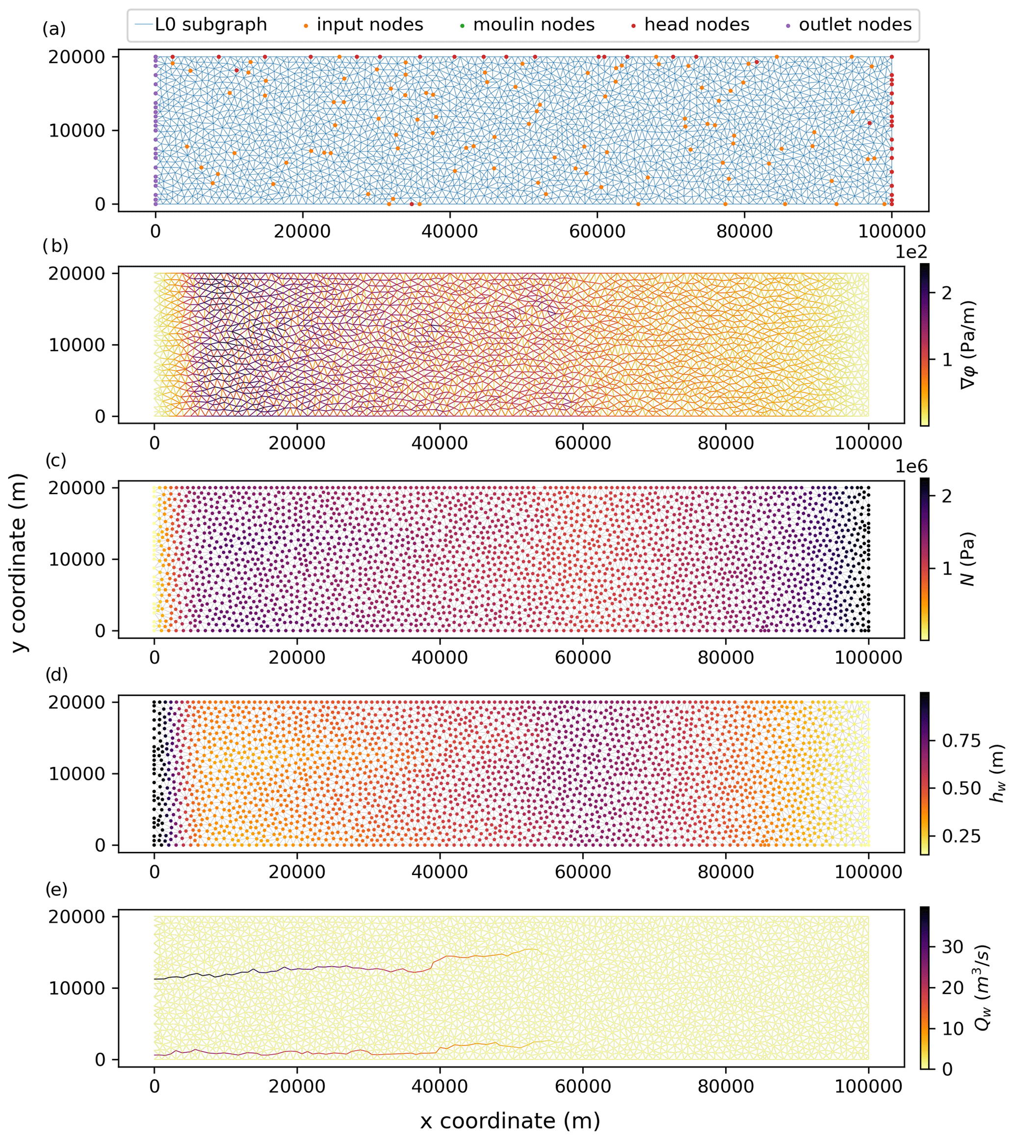
Figure 2 (a) The level 0 graph representation of the SHMIP model scenario A5 comprising edges on all valid paths. Head nodes are nodes with no predecessor nodes, and outlet nodes are defined at the grounding line. Input nodes are a randomly selected subset of nodes used to define the network geometry. This model scenario has no moulin nodes. (b) The hydraulic potential gradient defined on edges, (c) the effective pressure defined on nodes, (d) the thickness of the sheet h_w defined on nodes, and (e) the channelised water flux defined on edges.

3.1.1 Graph connectivity measures for effective hydrology representation

Subgraphs may be defined according to several criteria, but our principal goal is to define the most important edges for a given hydrology model scenario, in order to represent the channelised drainage system effectively and so to reduce the magnitude and complexity of the model. Edge weights are assigned according to the channel area, which is a robust feature of the GlaDS model (Eq. 8) and is closely linked to the magnitude of water flux and the channel width. For the weighted graph, we calculate edge betweenness centrality, which represents the relative frequency that each edge is found on the shortest paths between all source node–target node pairs (Brandes, 2001). For the problems here, we use the formulation

$$\begin{array}{}\text{(26)}& c_B\left(e\right)=\sum _{s,t\in V}{\displaystyle \frac{\mathit{\sigma }(s,t|e)}{\mathit{\sigma }(s,t)}},\end{array}$$

where V is the set of all nodes, s is the set of source nodes, and t the set of target nodes. σ(s,t) is the number of shortest paths for that node pair, while $\mathit{\sigma }(s,t|e)$ is the number of those that pass through the edge e. In this work, we normalise edge betweenness centrality as $\mathrm{1}/\left(\right|s\left|\right(\left|t\right|-\mathrm{1}\left)\right)$ where $\left|s\right|$ and $\left|t\right|$ are the total number of source and target nodes respectively. Therefore, a normalised edge betweenness centrality >0 means that the edge was on at least one shortest path, while an edge betweenness centrality of 1 implies that the edge is on every shortest path.

To define transport on the graph, it is necessary to have enough node pairs to represent the extent of valid flow paths. For maximal precision, all nodes can be used, but to reduce computation time, a sub-selection is used instead. Source nodes include all head nodes and moulin nodes and a random set of n input nodes to represent a spatially distributed hydrological input. Target nodes are the outlet nodes. In this case n=100 with 37 head nodes and 24 outlet nodes, giving ∼ 3000 shortest paths. A directed graph will be less-well-sampled upstream relative to downstream.

For a more focused representation of the high-flux channels using edge betweenness centrality, we define hierarchical subgraphs as views of the level 0 subgraph (Fig. 3). In this case, we define two further subgraph levels, with edge betweenness centrality >0 (level 1), comprising all edges on at least one shortest path, and >0.005 (level 2), comprising edges on 16 or more shortest paths. For example, in model scenario A5 (see Sect. 4), the level 1 subgraph includes 98 % of total channelised flow on 31 % of the edges, while the level 2 subgraph includes 97 % of total channelised flow on 20 % of the edges. Crucially, the high-flux edges are evolving dynamically with much higher sediment transport capacity, and so we may analyse these subgraphs more frequently than the main graph, reducing computation cost without the loss of precision. Besides computational benefit, the graphs for different model scenarios show a diversity of network characteristics that define how water (and sediment) are transported, with significant implications for understanding the sensitivity of sediment flow organisation to changes in the hydrological system.

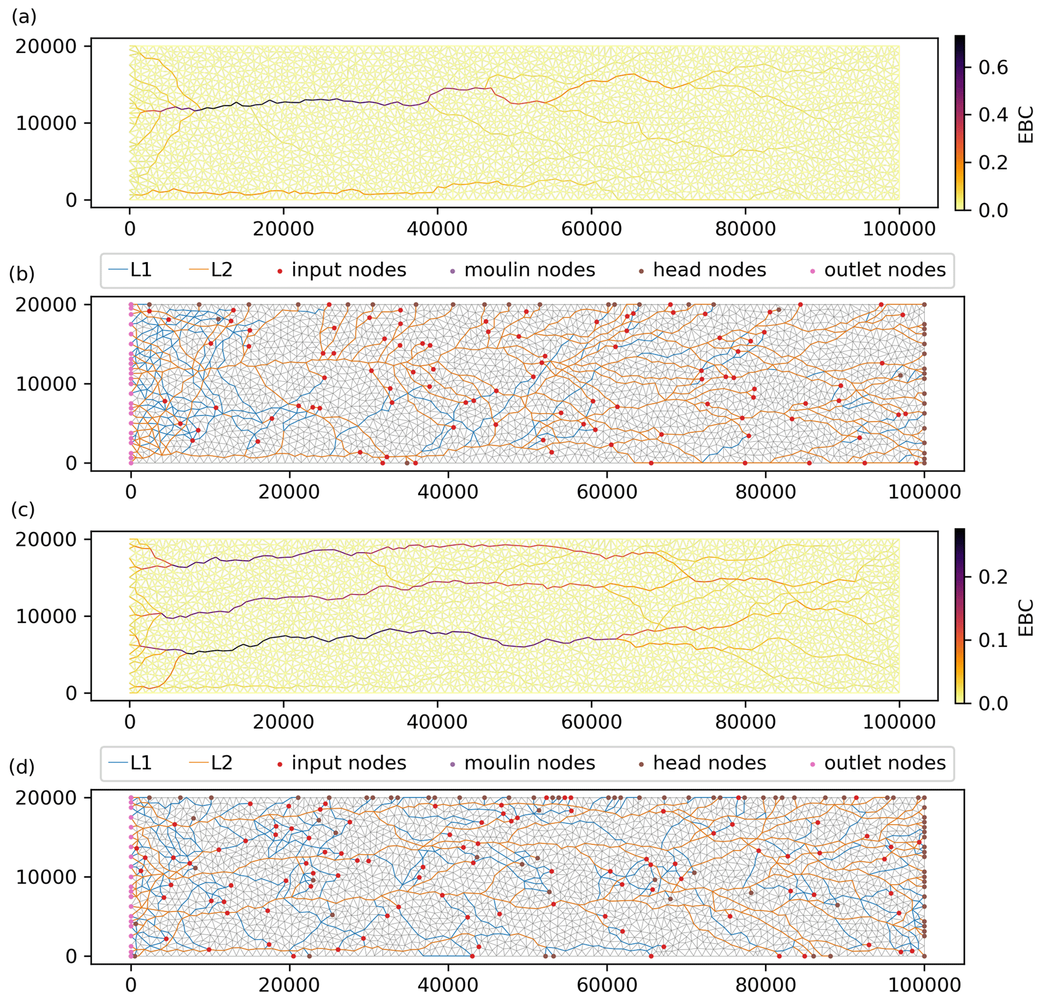
Figure 3 (a) Edge betweenness centrality (EBC) for the SHMIP model scenario A5 computed on the L0 graph: source nodes include moulins, head nodes, and randomly selected input nodes, while target nodes are the outlet nodes. (b) L1 and L2 hierarchical subgraphs derived from EBC thresholds of >0 and ≥0.005 respectively. Panels (c) and (d) show the same as (a) and (b) for model scenario A6. These examples do not have any moulin nodes.

3.2 Sediment modelling approach

In line with Sect. 2.2, we run the sediment transport model in several steps. For each model run, we initialise the graph with the grain-size distribution d50 and the basal sediment thickness as stochastic variables and with the grain density and erosion potential as constants. For each edge, we calculate local transport capacity as in Eq. (10) and sediment mobilisation as in Eq. (13). The network-scale transport model is applied, and we update the bed elevation and basal sediment thickness as defined in Eq. (15). The final, optional stage of the GraphSSeT model is to apply the detrital provenance tracking (Sect. 2.2.6).

For the grain-size distribution, we use a stochastic sampling procedure. For steady-state model runs, the grain-size distribution is seeded with a random number array that has for each edge (or node) at each time step a sample of size n=1000 drawn from the standard normal distribution (mean = 0; standard deviation = 1). The input seed array spans the first 2 weeks of the model time period, after which samples are drawn from a shuffled array. For non-steady-state model runs, every time step we draw a new sample for every edge (or node) from the standard normal distribution. To generate the real valued distributions, each sample is scaled by ς and offset by μ for the relevant distribution.

4 Model scenarios and model inputs for this study

To define controls on the subglacial fluvial sediment transport system, a series of experiments were conducted with synthetic model scenarios derived from the Subglacial Hydrology Model Intercomparison Project, SHMIP (De Fleurian et al., 2018). We do not wish to study here the hydrology model differences, and we consider only the examples computed with GlaDS.

Three series of SHMIP models were used. The A series represents a hydrologic steady state with a distributed water input to the sheet (m_b) applied at a constant rate and distributed equally across all nodes in the domain. The B series represents a hydrologic steady state with both distributed and focused water inputs. Only a small distributed water input to the sheet is included, while focused water input (m_s) is applied through moulin nodes at a constant rate but with differing intensities between scenarios. For these model scenarios, the hydrology network was developed dynamically over a time period of ca. 21 years. The C series represents a hydrologic non-steady state and involves time-varying water input to moulins on a diurnal cycle from $\frac{\mathrm{1}}{\mathrm{4}}$ to 2 times the base input. The C-series models build on the final state of the model scenario B5 with 100 moulins, and the hydrology network was developed over an additional time period of 50 d.

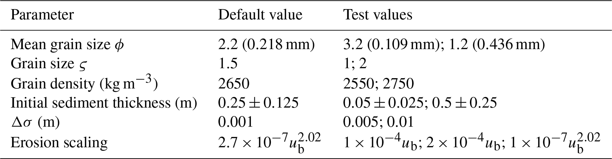
The base scenario is the model scenario A5, with water input to the ice sheet bed at a moderate level ($\mathrm{4.5}\times {\mathrm{10}}^{-\mathrm{8}}$ m s⁻¹ or ∼ 3.93 mm d⁻¹). Default experimental parameters and properties for our experiments are presented in Table 1. For steady-state model scenarios, the last time step of the hydrology model scenario was used to force the sediment model. Most model runs were conducted over a time period of 26 weeks, analogous to a summer season. The model run comprised daily cycles of 8 3 h time steps: the first and last use the level 0 subgraph, and in between a cycle of six time steps alternating between the level 1 and level 2 subgraphs is used. This cycle captures the potential for higher-flux channels to evolve more rapidly, while ensuring that the whole network is covered sufficiently often. For non steady-state model runs, the sediment model is a downsampling of the original hydrology model scenario time steps. This sampling need not be linear, but in this case, the hydrology model state was reported every hour, and we ran the sediment models at this sample interval.

Experiment set 1 was conducted for the A-series model scenarios with default parameters to demonstrate the effect of increasing basal water supply to the model. Experiment set 2 was conducted with the model scenario A5 and establishes the sensitivity to major parameters, including the initial basal sediment layer thickness, the erosion scaling, Δσ, the grain-size distribution, and grain density. Experiment set 3 considers the effect of focused water input using the B-series model scenarios, while experiment set 4 considers diurnally time-varying water input using the C-series model scenarios. Finally, we demonstrate several model runs with the bedrock detrital provenance tracking mode enabled.

4.1 Reference and default models

For each hydrology model scenario, we ran a reference model scenario with no grain-size variation and two model runs with default parameters. The default model has an initial randomly defined basal sediment thickness of 0.25±0.125 m and erosion scaling set to $\mathrm{2.07}\times {\mathrm{10}}^{-\mathrm{7}}{u}_{\mathrm{b}}^{\mathrm{2.02}}$ (Herman et al., 2018). The mean grain size is $\mathit{\varphi }=\mathrm{2.2}\approx \mathrm{0.218}$ mm and ς=1.5, corresponding to typical grain-size distributions of subglacial till (Peterson et al., 2018; Haldorsen, 1981). The reference model scenario has the same variables as the default except that ς is zero.

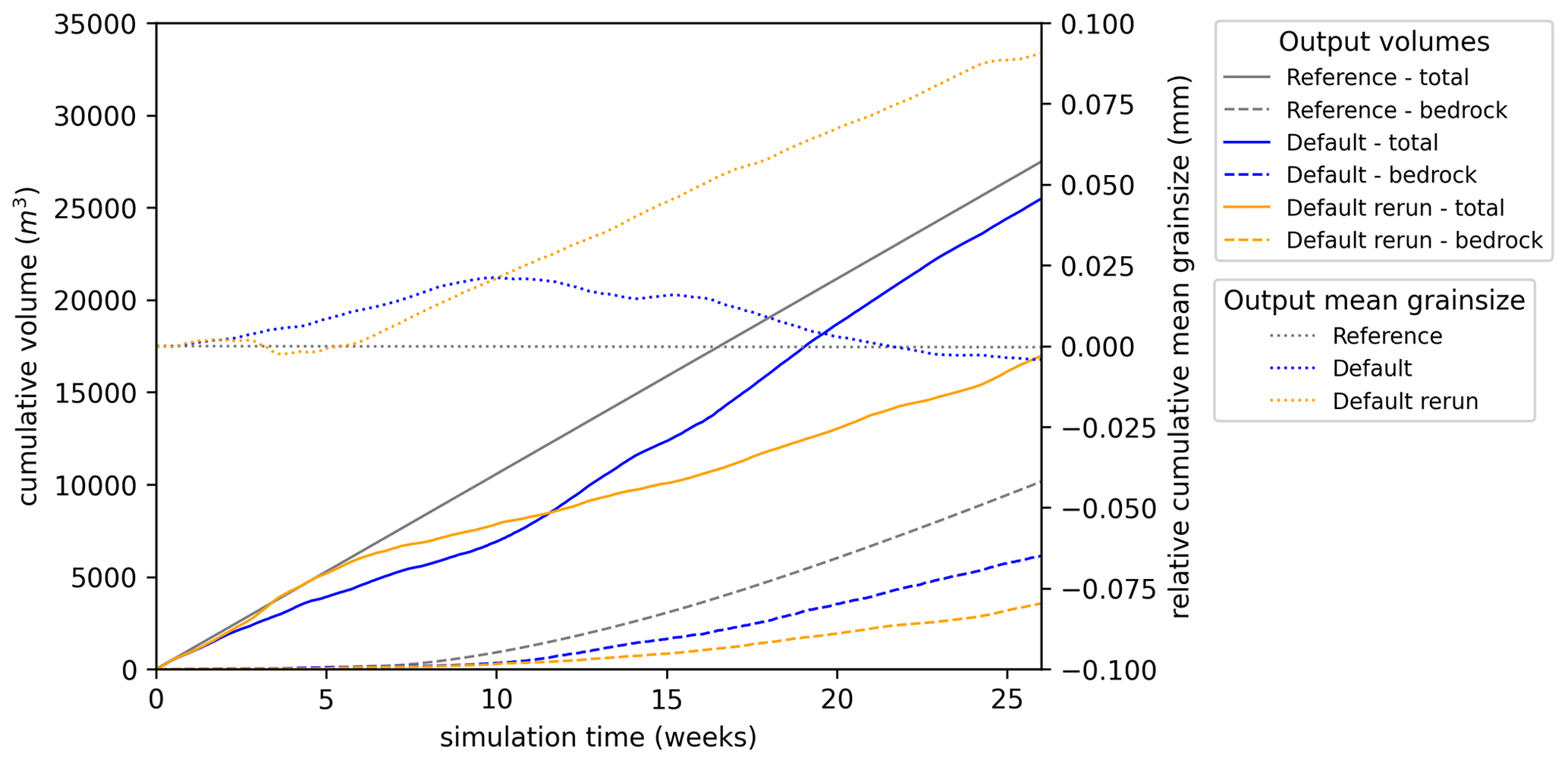
Figure 4 The reference run and two separate runs with default parameters, all using the hydrology model scenario A5. For each, solid lines show the cumulative total sediment discharge, and dashed lines show cumulative bedrock sediment discharge derived directly from erosion of bedrock. The difference is the cumulative sediment discharge from remobilised basal sediments. Dotted lines show cumulative mean grain size relative to the initial mean.

The hydrology model scenario A5 generates two major channels, one in the south of the model and the other more central, which has greater flux (Fig. 2e). Edge betweenness centrality subgraphs define a linear–dendritic network geometry comprising numerous minor channels convergent with the major channels along their length and a divergent network near the outlet nodes. This divergent network accommodates the pathways for flow to all outlet nodes (Fig. 3a). The reference model run generates a nearly constant sediment discharge rate at the outlet nodes (Fig. 4), representing the combined transport capacity of the outlet edges. Total sediment discharge over 26 weeks for the reference model is 2.75×10⁴ m³, with the vast majority from the central subglacial channel. The default models show significant variations in sediment discharge rate, occurring in line with the grain-size distribution (Fig. 4). In these model runs, the initial basal sediment layer is rapidly removed along the major channels, which subsequently remain largely sediment free, but more widespread mobilisation of sediment does not occur. The proportion of bedrock-derived sediment consistently increases from ca. 5 weeks on.

4.2 Experiment set 1

In experiment set 1, we compare the impact of steady-state GlaDS scenarios with variable basal water input, run with default parameters. SHMIP model scenario A4 considers a low level of basal water input of 2.16 mm d⁻¹ and represents threshold conditions for channelised flow. SHMIP model scenario A6 has a much greater input of 50 mm d⁻¹, representing peak water discharge driven by surface melt in Greenland-like conditions (De Fleurian et al., 2018). Two additional GlaDS models were run in between A5 and A6, with flux rates of 21.6 (A7) and 39.3 mm d⁻¹ (A8). The network geometry of all these models is linear–dendritic, with the development of more closely spaced and longer channels as flux increases (Fig. 5).

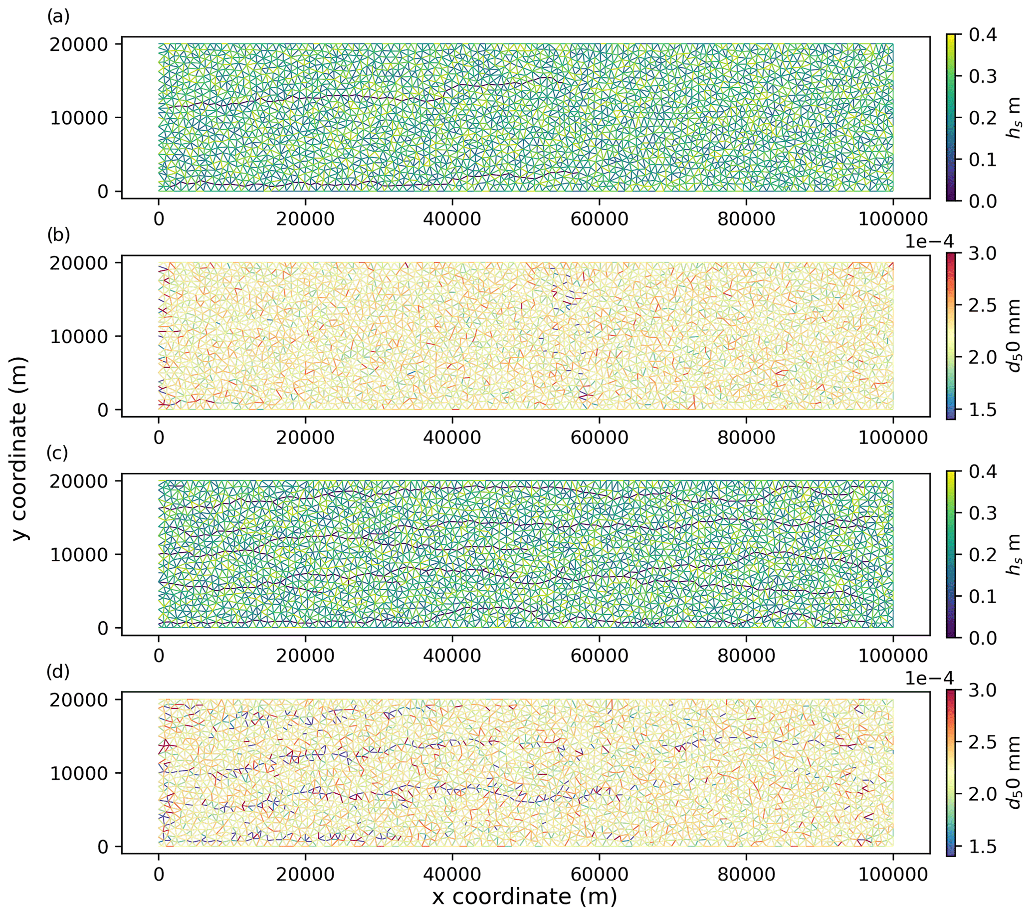
Figure 5 (a) Sedimentary layer thickness and (b) median grain size at the end of the A5 default model run. Panels (c) and (d) show the same for the A6 default model run. Note the selective transport for model A6 with finer-grained sediment in the major channels.

These model scenarios generate substantially different conditions for sediment transport, with total sediment discharge for the default A4 model just 1.79×10³ m³, 2.55×10⁴ m³ for A5, and 4.60×10⁵ m³ for A6; the intermediate models A7 and A8 generate discharge of 1.01×10⁵ and 3.72×10⁵ m³. Grain-size evolutions for the higher-flux model runs show a consistent pattern of initially flat or increasing grain size for 5–10 weeks, followed by a systematic reduction in grain size. These variations in grain size are associated with variations in sediment discharge (Fig. 6). The interpretation is that for higher-flux model runs, the selective transport of finer-grained material from upstream increases discharge rates by increasing sediment transport capacity. Lower-flux model runs show no such grain-size reduction, indicating that selective transport is not as significant in low-flux conditions.

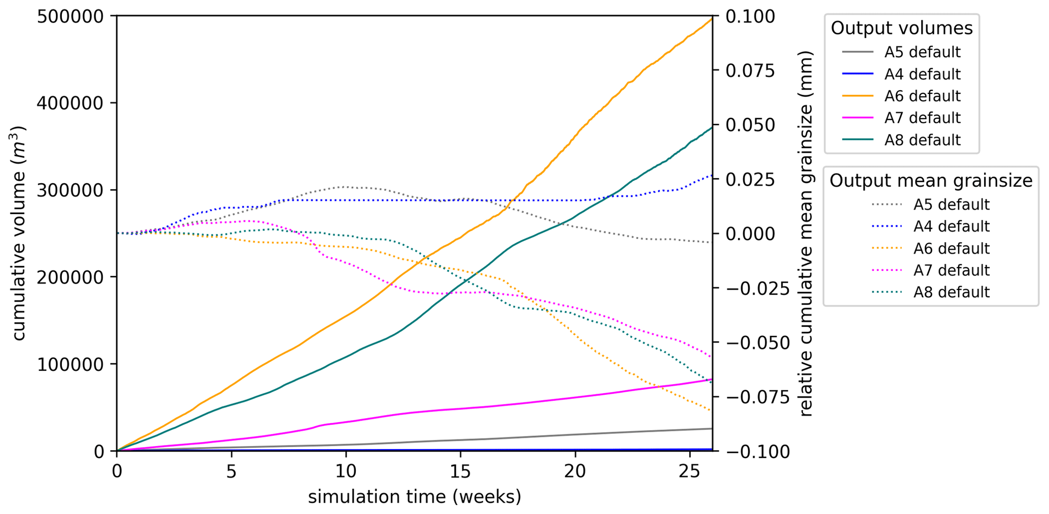
Figure 6 Sedimentary output for all the models of experiment set 1 with default settings. For each, solid lines show the cumulative total sediment discharge, and dotted lines show cumulative mean grain size relative to the initial mean.

4.3 Experiment set 2

Table 1 Tested parameters in experiment set 2, conducted with the model scenario A5.

4.3.1 Grain-size distribution and its variance

In experiment set 2, we vary selected input parameters from the default parameters (Table 1) to gauge their importance for sediment transport. Grain size is fundamental to both transport capacity (Eq. 10) and transport velocity (Eq. 18) and also varies naturally across several orders of magnitude (Peterson et al., 2018; Haldorsen, 1981). Here, we test the impact of this parameter, varying both μ and ς of the population distribution. In the former case (Fig. 7a), we see the profound impact of the value of μ: overall discharge for a mean of ϕ=1.2 (grain size 0.436 mm) is 7.96×10³ m³, but with a mean of ϕ=3.2 (grain size 0.109 mm) discharge is 6.25×10⁴ m³. Changes in the grain-size distribution during the model run indicate that selective transport occurs for the finer-grained model runs, causing a reduction in grain size from 10–15 weeks; however, the coarser-grained model run does not show evidence of selective transport developing (Fig. 7a).

The variability in grain size is also significant with higher variance associated with increased discharge and finer at-outlet grain size, while lower variance is associated with reduced discharge and coarser at-outlet grain size (Fig. 7b). The interpretation is that samples with a coarser median grain size will reduce transport capacity and the associated sediment volume can only be transported slowly. In contrast, samples with finer median grain size should be transported rapidly through the network. Consequently, while higher variance will develop coarse- and fine-grained samples equally, only the fine-grained samples will propagate through the graph and influence discharge at the outlet. In Fig. 7b with ς=2, strong selective transport reduces the grain size markedly from ca. 10 weeks onwards, while for ς=1 the grain size increases steadily.

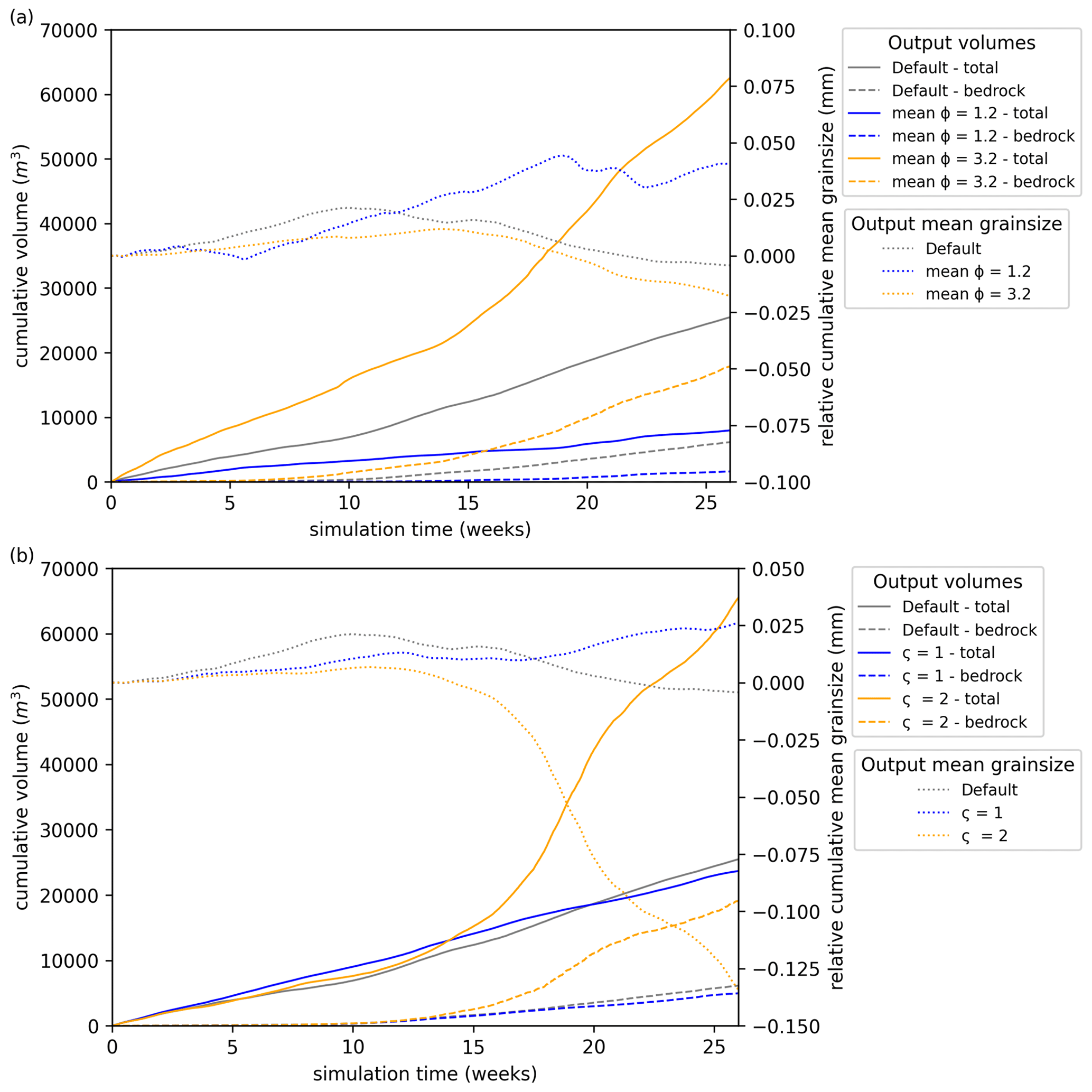
Figure 7 Sediment output with variations in (a) grain-size distribution mean and (b) grain-size distribution standard deviation, using scenario A5. For each, solid lines show the cumulative total sediment discharge, dashed lines show cumulative bedrock sediment discharge derived directly from erosion of bedrock, and dotted lines show cumulative mean grain size relative to the initial mean.

Grain density is in principle a very important factor for sediment transport capacity (Eq. 10), but due to a relatively limited range, its effect is minor in comparison to the grain size. The influence of higher and lower grain density was tested and showed that the model run with lower grain density is not associated with increased discharge overall, while the model run with higher grain density is associated with moderately reduced discharge. This deviation may be explained by changes in grain size rather than necessarily a direct impact of grain density. Overall, grain density does not lead to large variations in either the sediment discharge volume or grain size at the outlet nodes.

4.3.2 Basal sedimentary layer thickness and Δσ

The thickness of the initial basal sediment layer is important for sediment transport because this material is available to be mobilised whenever transport capacity exceeds supply from erosion. We tested the impact of this initial condition with reduced initial thickness of 5±2.5 cm and increased initial thickness of 50±25 cm (Fig. 8). For these model runs, higher initial sediment thickness results in increased total discharge (Fig. 8). Although we may expect enhanced supply for greater initial thickness, the effect is in line with the expected impact of grain-size variations. More significant are the delay in the onset of bedrock erosion to 15 weeks in the high initial thickness run and a much lower proportion of bedrock-derived sediment (Fig. 8).

Sediment mobilisation is modulated by the parameter Δσ, which controls the transition between the supply-limited and transport-capacity-limited regimes (Eq. 13c). Increases of Δσ=0.005 m and Δσ=0.01 m caused little variation in the overall sediment discharge but had a marked effect in reducing the proportion derived from the bedrock. The importance of the basal sediment layer is not only increased supply but also protection of the bedrock from erosion. Along with h_s, h_max and Δσ control access to the bedrock. Higher values for h_s and Δσ sustain the basal sediment layer for longer. This enhances potential sediment supply and reduces the proportion of bedrock-derived sediment. Higher values for h_max will tend to increase the proportion of bedrock-derived sediment. Furthermore, in the case of deposition and remobilisation, a greater volume of basal sediment acts as a buffer in grain-size mixing calculations, which may influence grain-size evolution and selective transport. Although important, the basal sediment layer had, for this model scenario, a small overall effect on the volume and grain size of sediment discharge.

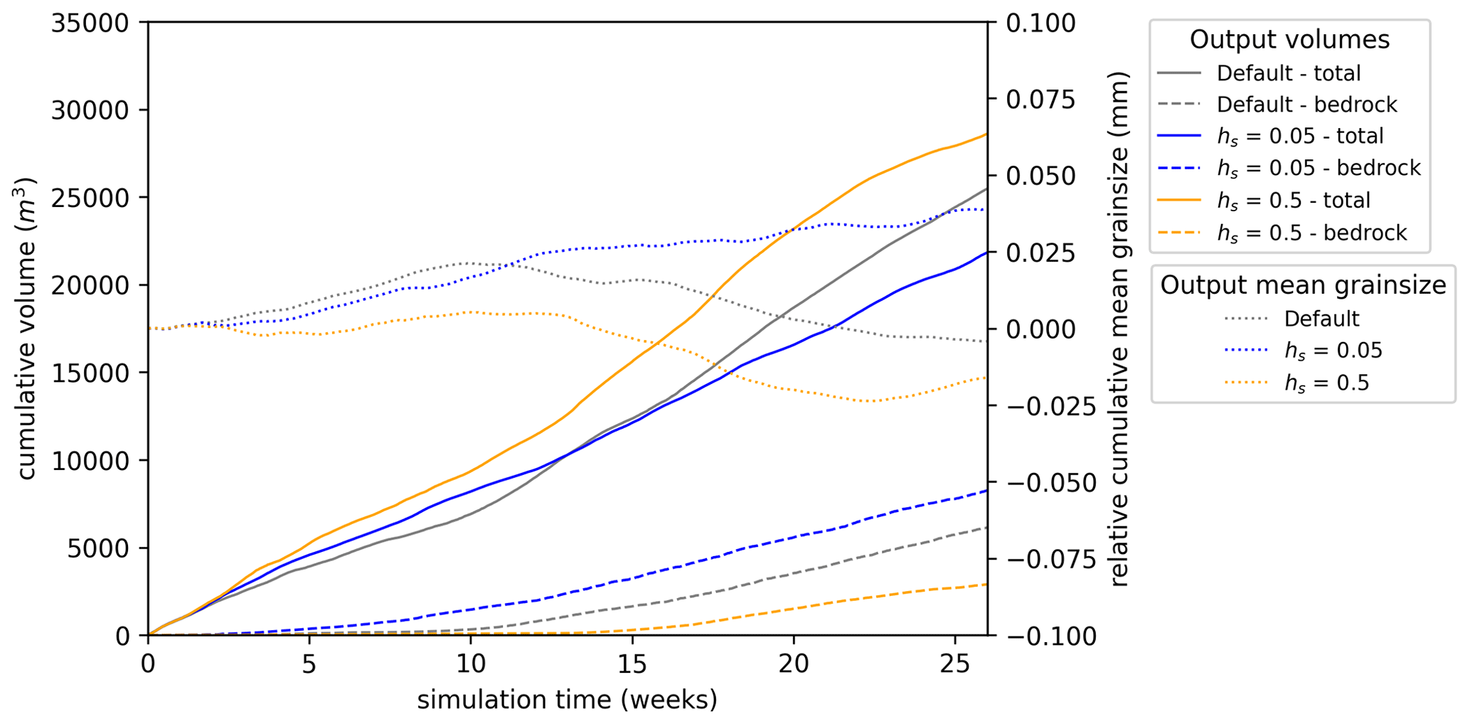
Figure 8 Sedimentary output with variable initial basal sediment layer thickness h_s, using scenario A5. For each, solid lines show the cumulative total sediment discharge, dashed lines show cumulative bedrock sediment discharge derived directly from erosion of bedrock, and dotted lines show cumulative mean grain size relative to the initial mean.

4.3.3 Erosion law scaling

The supply-limited regime and its distinction from the transport-capacity-limited regime are fundamentally constrained by the rate of bedrock erosion (Eq. 12), which in GraphSSeT is controlled first by the protective effect of the basal sediment layer, second by the basal ice velocity (in this case, a constant at $\mathrm{1}\times {\mathrm{10}}^{-\mathrm{06}}$ m s⁻¹), and third by the choice of erosion scaling law. Velocity-based erosion scaling laws with linear and velocity-squared laws are both common, although other exponents are possible (Herman et al., 2018, 2021; Cook et al., 2020). For our model scenario with velocity-squared scaling, reducing the pre-exponent had little effect on the model (Fig. 9). The linear scaling, in general, provided additional discharge and showed greater sensitivity to the scaling parameter (Fig. 9). However, the effect is much less marked than the variation in the erosion potential itself, which is a factor of ∼ 30–60 times greater. The interpretation is that the effects of basal sediment thickness and capacity-limited transport restricted the influence of erosion potential. More generally, if the system is transport-capacity-limited and has an extensive basal sediment layer, then erosion potential will have a limited impact on sediment discharge. The effect on supply is seen in the bedrock-derived sediment, which has a greater volume proportion and earlier onset with the linear scaling law (Fig. 9).

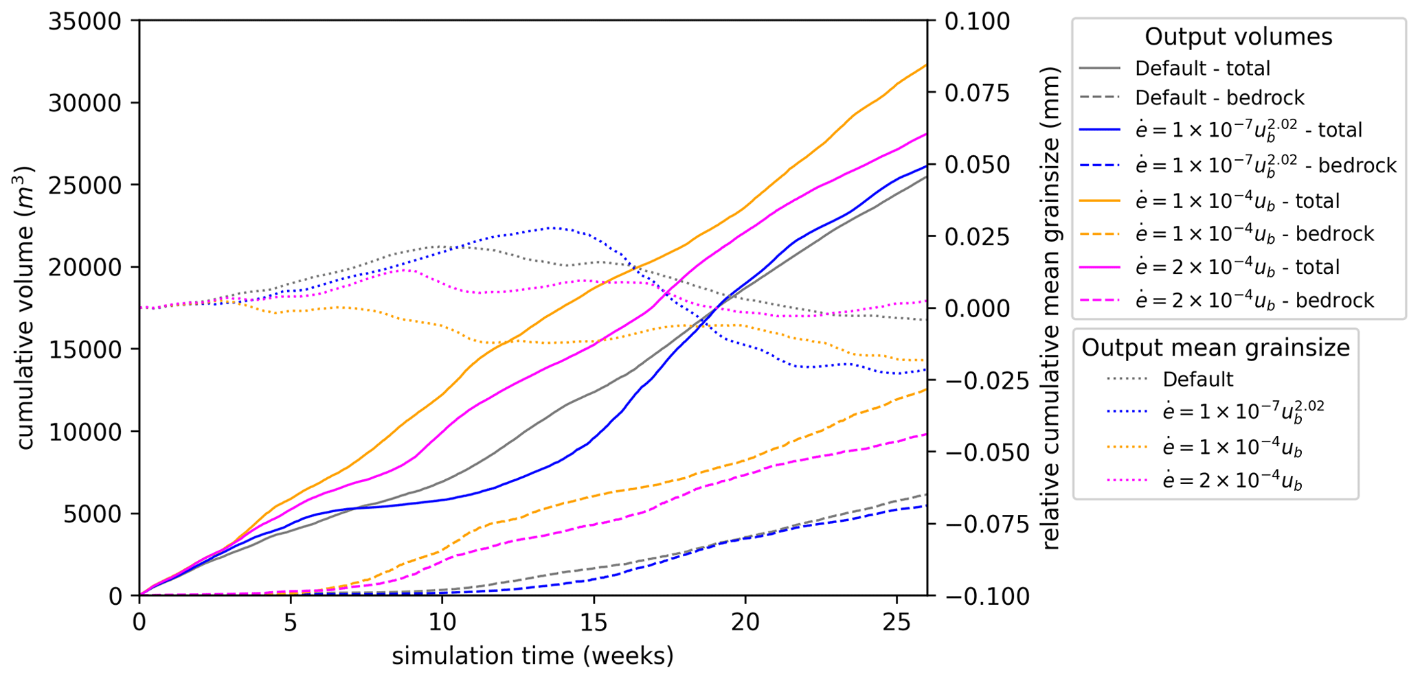
Figure 9 Sedimentary output with different erosion scaling laws using scenario A5. Scaling laws are for velocities expressed in metres per annum. For each, solid lines show the cumulative total sediment discharge, dashed lines show cumulative bedrock sediment discharge derived directly from erosion of bedrock, and dotted lines show cumulative mean grain size relative to the initial mean.

4.4 Experiment set 3

In experiment set 3, we investigated the influence of concentrated hydrological inputs with a scattered distribution (De Fleurian et al., 2018). In this experiment set, the volumetric water input is identical to the A5 model scenario but comprises only a small distributed basal input (0.006 mm d⁻¹), with the remainder split between n randomly selected input nodes representing moulins. Models B1 through B5 investigate this flow for n=1 to n=100, with a corresponding volumetric water input of 90 to 0.9 m³ s⁻¹ for each. For each of these model scenarios, we ran four sediment transport model runs. The results indicate that the distribution and intensity of focused water inputs are significant for sediment flux. The least sediment discharge occurs for the model scenario B1, with total discharge consistently below 5000 m³. B1 has a single moulin that yields a single channel but is not effective in accessing the bed more broadly. The other model runs return variable sediment discharge, but in general the greatest discharge occurs for model B2, while B4 tends to have the least (Fig. 10). These model runs have typically lower discharge than the runs for model scenario A5.

These model scenarios have only small differences in water flux at the outlet and in total channel volume, but they do have significant differences in the distribution and extents of channels, and these are interpreted to dictate the sediment transport. First, relative to model runs for scenario A5, the channel geometry is less well connected from the outlets to the inland areas of the domain, thus limiting the area exposed to channelised flow. Second, the main channels typically have reduced water flux. These combined effects lead to generally lower and more-variable sediment discharge for a given total water input.

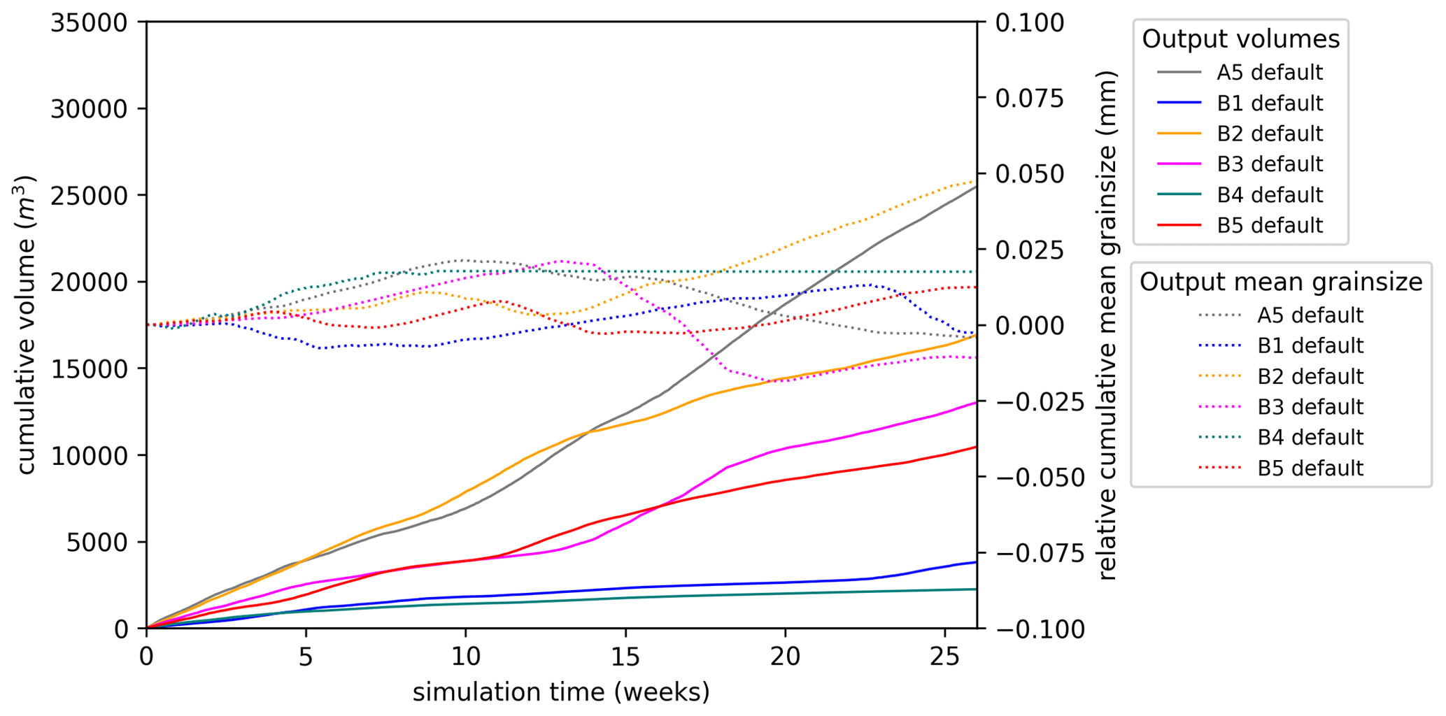
Figure 10 Sedimentary output for the default models of experiment set 3. For each, solid lines show the cumulative total sediment discharge, and dotted lines show cumulative mean grain size relative to the initial mean. Bedrock components are not shown.

4.4.1 Experiment set 4

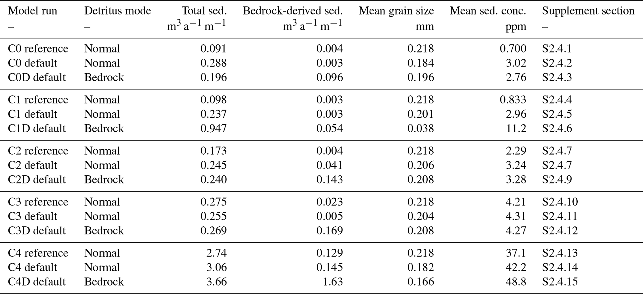
For experiment set 4, we investigate the influence of non-steady-state hydrology with a diurnal time-variable input over a period of 50 d. The total volumetric input and the locations of the moulins are identical to the model scenario B5, but the input is varied according to a diurnal sinusoidal cycle,

$$\begin{array}{}\text{(27)}& R(t,R_{\mathrm{a}})=max\left(\mathrm{0},m_{\mathrm{s}}\left[\mathrm{1}-R_{\mathrm{a}}\sin \left({\displaystyle \frac{\mathrm{2}\mathit{\pi }t}{s_{\mathrm{d}}}}\right)\right]\right),\end{array}$$

where t is the time in seconds, s_d is the number of seconds per day, and m_s=0.9 m³ s⁻¹. The amplification factor R_a is tested across a range from 0.25 (C1) to 2 (C4), noting that for R_a>1 it is necessary to truncate the function to remain non-negative (Eq. 27). This leads to a slight increase in total flux volume for the model scenario C4. In addition to these, we run a C0 model that uses the same run procedure but without any diurnal variation.

For these runs, the sediment model is run with some modifications to the approach. With variable hydrology, edges may change status during the run (e.g. by becoming ungrounded), or flow directions may be reversed. This demands that a fresh graph is constructed for each time step, and from this graph we recompute edge betweenness centrality and generate the desired subgraph. In this way, the network geometry dynamically evolves with the hydrology model. We run the model with a 1 h time step, in line with the hydrology model outputs, and each day run 8 cycles of three iterations, these being run on the L2, L1, and L0 graphs, in that order.

The results (Fig. 11) indicate that the magnitude of the diurnal cycle impacts sediment flux such that higher intensity in the diurnal cycle is associated with increased sediment discharge during periods of peak water input, while the corresponding reduction during low-input periods is limited. The increased discharge is due to increased sediment concentration during daily peak flow, which reaches 60–100 ppm in the C4 runs versus peaks of 10–30 ppm for the C1 runs. The relationship is consistent with increased transport capacity at peak flow due to increased basal shear stress from fast water flow, in line with Eq. (10).

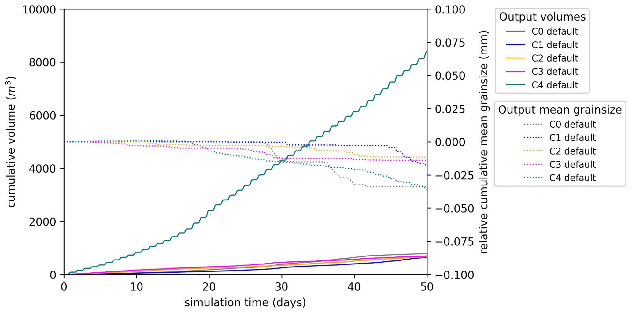
Figure 11 Sedimentary output for the models of experiment set 4. For each, solid lines show the cumulative total sediment discharge, and dotted lines show cumulative mean grain size relative to the initial mean.

4.4.2 Detrital examples

For these model runs, we track the detrital property of bedrock class through the network. For our bedrock classification we use here a graticule (Fig. 12a) with five classes from the front to the back (0, 1, 2, 3, and 4) and three classes across the model width (L, C, and R). These classes represent spatial areas of the same size but in principle could be any property the user wishes to track (for example bedrock geology). Material eroded from nodes possessing the detrital property is assigned to the associated class for the purpose of detritus tracking.

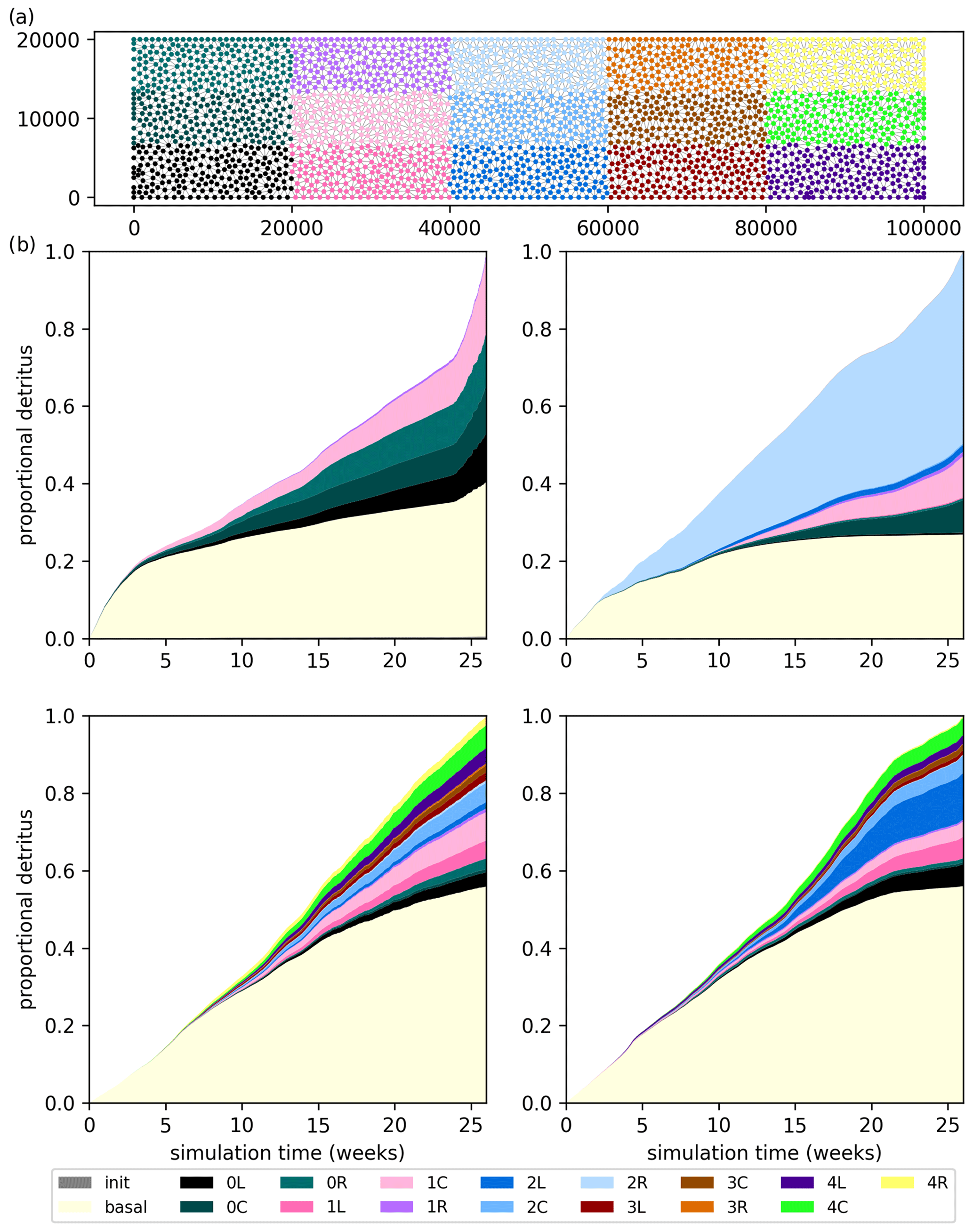
Figure 12 (a) Map of graticule classes. Panels (b) to (e) show stack plots of cumulative volume by class as a proportion of total volume for the model runs A4D, A5D, A8D, and A6D. The class init represents initial active sediment on edges, and basal represents the initial basal sediment layer; neither of these is associated with spatial location.

The distribution of detritus for these model runs indicates significant differences in the erosion, mobilisation, and transport of detritus. Systematic changes are seen in the degree of access to inland classes between models (Fig. 12). For these model scenarios, erosion potential is uniform throughout, and thus the differences seen are due to bed access through sediment cover and to the effectiveness of the transport system.

In all cases, the early part of the model run is dominated by mobilisation of basal sediment, the volume of which reduces significantly during the model run as the initial basal sediment is depleted. For model run A4D, the hydrology network is limited in inland extent, and bedrock-derived detritus is dominated by the classes 0L, 0C, and 0R, reflecting transport at the margin, but with some class 1C due to the central channel. For model run A5D, the detrital signature is different, with the classes 2R 1C, and 0C dominant. These classes underlie the main channel where bedrock is exposed (Fig. 5). Moreover, the dominant class is 2R transported from the upstream catchment: as is expected from Eq. (13), transport of incoming active sediment is prioritised over eroded or remobilised sediment, and thus the downstream classes 1C and 0C are subordinate (Fig. 12). High-flux model runs A8D and A6D are markedly different to the preceding, with first a greater proportion of detritus from basal sediment and second a much more uniform sampling of bedrock classes. This indicates a much-broader sampling of the bed, extending across almost the whole domain. Model run A6D has an enhanced pulse of detritus from class 2L from weeks 15 to 20. This corresponds to a period of low grain size, suggesting a strong grain-size-driven selective transport event stemming from that region and propagating to the outlet.

5 Discussion

5.1 Geological controls on sediment flux

The dominant geological factor is grain-size distribution, which controls transport capacity variations and in particular drives the evolution of selective transport. The transport system self-organises in response to stochastic variations in grain size: coarser grain sizes are not transported efficiently and tend to move slowly through the network; smaller grain sizes are preferentially transported and will tend to progress rapidly through the network. A tendency is seen in many of the model runs for increasing grain size early in the run (up to ca. 10 weeks) and then for most higher-flux runs a systematic reduction in grain size. In contrast, most of the lower-flux model runs do not show any decrease in grain size. The evolution may be explained by the ice sheet geometry, with a region of high potential gradient from 5 to 20 km upstream (Fig. 2) in which relatively coarse-grained sediment can be transported. The coarser-grained sediment can only be transported off the network slowly. In model runs with higher flux, finer-grained sediment is transported from further upstream due to selective transport, leading to a significant increase in transport capacity through time.

The thickness of the basal sediment layer is a key factor for sustained sediment supply and controls access to the bedrock (Delaney and Adhikari, 2020). A further effect of basal sediment thickness occurs during the mixing of sediment, as this layer is an important buffer for the evolving grain-size distribution and through this exerts further control on sediment transport dynamics. In particular, the onset of volumetrically abundant bedrock-derived detritus is in many model runs coincident with significant reductions in the at-outlet grain-size distribution. This is a consequence of the feedback between transport capacity, mobilisation, and grain-size buffering. Under selective transport, sediment flowing into an edge will often have a finer grain-size distribution than the residual sediment, which will increase the transport capacity and is likely to cause remobilisation of basal sediment. In most cases, this will be coarser grained and so partially offset the increased transport capacity, but as basal sediment is lost, the buffering effect of this layer is reduced and thus the selectivity of the transport system is enhanced. For coarser-grained incoming sediment, the reverse effect is expected, and the drop in transport capacity will lead to deposition and coarsening of the basal sediment, leading to inhibited flow through the edge until sufficient finer-grained sediment arrives.

5.2 Glaciological controls on sediment flux

In our experiments, varying the erosion potential scaling law had a limited impact on sediment flux, as this factor is subordinate to the effects of the basal sediment layer and because the model runs are transport-capacity limited. As a consequence, the composition of detritus reflects variations in transport rather than in supply. This suggests that for correct representation of the detrital signatures of glaciers and ice sheets, it is critical to understand transport as well as erosion (Aitken and Urosevic, 2021). Our input model scenarios have no topography; no spatial variations in ice-sheet basal velocity, bed roughness, or bedrock erosive properties; and therefore no variation in erosion potential. In the general case, variable erosion rates may occur due to variations in basal sliding velocity, in bedrock roughness, and in erodibility of the bedrock (Alley et al., 2019). A secondary effect is the potential impact of variations in bedrock lithology, joint frequency, and structure orientation on at-source grain-size distribution (Krabbendam and Glasser, 2011; Hooyer et al., 2012). Variations in erosion rates and at-source grain-size distributions would cause both sediment supply and transport capacity to vary in ways that might significantly impact network-scale transport dynamics.

5.3 Hydrological controls on sediment flux

5.3.1 Water input controls on sediment flux

Experiment set 1 assessed the effect of basal water input on the discharge of sediment. For lower quantities of basal water input, the channel system is less extensive, but with higher quantities of basal water input, these channels become more numerous and extend further inland. With no topography or other constraints on these model scenarios, the network geometry self-organises to form linear–dendritic channel networks with little interaction between channels (Hewitt, 2011). In the model scenarios, the overall relation of sediment discharge to basal water input scaled linearly with the total channel volume. Across all model runs, the best-fit scaling per unit width was $Q_{\mathrm{s}}\approx \mathrm{0.042}\sum {\mathrm{Sl}}_{\mathrm{edge}}-\mathrm{1.28}$ m³ a⁻¹. While low-flux model scenarios have minimal channelisation and low sediment discharge, higher-flux scenarios have extensive and well-formed hydrology networks. These networks have much-greater capacity to access the bed and to mobilise sediment across the broader domain (Figs. 5 and 12), leading to an increase in sediment discharge.

Experiment set 4 tested the effect of diurnal variations in water input via moulins. The model runs in this suite typically generated additional sediment flux relative to an identical series run without temporal variation. Furthermore, the greater the variability, the greater the sediment discharge – in particular for model C4 (Fig. 11). Due to limited capacity of the channel geometry to adjust to short-term variations in water input, water velocity within the channels will increase, causing transient peaks and troughs in sediment transport capacity and therefore discharge. Furthermore, while the discharge peaks may be significantly higher than the background level, the corresponding troughs have little influence on total sediment discharge, and thus systematically higher total sediment discharge is seen.

5.3.2 Network geometry controls on sediment flux

Experiment set 3 tested the effect of different configurations of moulins on the sediment flux, from broadly scattered inputs (100 moulins) to highly focused inputs (1 moulin), with the same overall flux distributed between them in each case. The single-moulin model provided an exceptional result: one major high-volume channel develops but with little capacity to access the bed outside of this channel, and sediment discharge is always small. Sediment discharge for the other results were highly varied but were reduced relative to the model runs for the scenario A5. The configuration of moulin inputs is accompanied by significant changes in the network flow configuration, with less-extensive channel distributions and less-well-connected networks. The interpretation is that the extent and connectivity of channels is a limiting factor for efficient sediment transport at network scale. In the absence of other constraining factors, a completely distributed input will naturally self-organise with respect to forming regularly spaced channels and flow discrimination into catchments within which flow connectivity is high (Hewitt, 2011), generating an efficient sediment transport network. With a network involving higher flux at predefined input locations, network geometries must adjust to hydrological inputs that may not be conveniently located with respect to the development of a channelised flow network (Gulley et al., 2012), and so the capacity to mobilise and transport sediment effectively at the network scale is inhibited.

5.4 Comparison with observational data

We compare our sediment discharge to estimates of total sediment flux from glacial systems around the margins of Greenland, estimates of which exist for Petermann Glacier (between 1080 and 1420 m³ a⁻¹ m⁻¹ Hogan et al., 2012) and Jakobshavn Glacier (1030–2300 m³ a⁻¹ m⁻¹ Hogan et al., 2011) and more general estimates of which exist in the range of hundreds to thousands of cubic metres per annum per metre. In contrast, total sediment discharge from our model runs is typically below 50 m³ a⁻¹ m⁻¹, substantially less than observed volumes. We infer the low volumetric output of these model scenarios to be due to a very small catchment size relative to natural systems, being only 2000 km² versus tens of thousands of square kilometres for the catchments above.

Looking to sediment concentration, in the steady-state models, the mean volumetric sediment concentration varied between 0.5 to 90 ppm and was in the range of ∼ 20–30 ppm for most model runs. For a grain density of 2650 kg m⁻³, these concentrations correspond to a range of ∼ 1.3 to 240 mg L⁻¹ but were typically in the range of 50 to 80 mg L⁻¹. Concentrations during high-flux periods were potentially much higher, often in the range of 200 to 400 ppm (or 500 to 1000 mg L⁻¹). Overall, the sediment concentrations are within expected ranges for subglacial meltwater plumes reported in the literature (Chu et al., 2009; Schild et al., 2017; Overeem et al., 2017)

5.5 Model performance and development

5.5.1 Limitations and further development

The model runs presented here have addressed the main drivers of subglacial fluvial sediment transport with multi-diurnal to seasonal synthetic scenarios. We do not include any long-term runs for which new drivers are superimposed on the above. For example, sustaining ongoing sediment supply becomes a more critical condition (Delaney and Adhikari, 2020), while seasonal to multi-annual variations in hydrology superimpose additional variability on model forcing that may cause systematically different sediment transport conditions. Furthermore, we do not include topography, which is critical for hydrological flow organisation and will significantly control hydrology network geometry and flow routing (Hiester et al., 2016). Variable ice sheet flow through space and time will also impact channelisation and erosion and may be a significant driver of variable sediment supply. The application of subglacial hydrology models to real systems carries some additional challenges, including greater model size and complexity; multi-catchment structure; and the potential presence of hydraulic sinks, lakes, and diffuse, time-variable grounding zones. The current model design is sufficient to address all of the above, and these are being addressed further in applications of GraphSSeT to systems in Greenland and Antarctica.

In the preceding, GraphSSeT used semi-circular R-channel geometry consistent with the GlaDS hydrology model and therefore assumes a flat-bedded channel to calculate basal shear stress and sediment transport capacity (Eqs. 9 and 10). In addition, the mean water velocity is used. In principle, GraphSSeT may accommodate any channel geometry for which the basal shear stress can be determined, potentially including rectangular, U-shaped, and V-shaped incisions into the sediment layer, should these be compatible with the subglacial hydrology model used as forcing.

Grain-size-dependent transport has emerged as a key component of the transport model, with high sensitivity to changes in the grain-size distribution causing selective transport and non-linear behaviour. More tightly constrained grain size may in principle allow more consistent results, but this is unrealistic for glacial sediments that are generally unobserved due to ice cover and in any case are characterised by highly variable grain size (Haldorsen, 1981). Alternatively, model ensembles are needed to mitigate the impact of the stochastic grain-size variations and to define with greater accuracy the expected sediment volume and characteristics for the glacial–hydrological scenario of interest. One limitation of the model presented here is that although multimodal grain-size distributions are likely to develop through mixing processes, these will be poorly represented by the unimodal grain-size distributions used in this implementation. A Gaussian mixture model or a cumulative probability distribution approach could allow multi-modal distributions to be accommodated within the model design.

5.5.2 Computational considerations

Model development has not yet emphasised computational performance; however, some discussion is warranted. All model runs were conducted on a laptop with a 1.7 GHz processor (AMD Ryzen 7 PRO 4750U) and 32 Gb RAM, without parallelisation implemented. Run times were between ca. 1.5 and ca. 4.5 h. Average compute times per time step were ca. 4 s for steady-state hydrology runs with normal detritus tracking, increasing to ca. 4.5 s with bedrock detritus tracking. For non-steady state models, an average time step took ca. 9 s, increasing to ca. 10.5 s with bedrock detritus tracking.

The largest factor in run times was the size of the samples in the grain-size mixture calculations, for which a conservative choice of n=1000 was used here to mitigate excessive non-linear behaviour. A smaller sample size will yield significantly reduced run times but with a greater variability in model outcomes. Significant potential exists for this performance to be improved through parallelisation and optimising the procedure for large-scale ensemble models run on high-performance computing infrastructure.

6 Conclusions

We have developed a graph-based model, GraphSSeT, to represent subglacial hydrology networks and to calculate subglacial fluvial sediment transport through those networks. The model uses the output of a subglacial hydrology model, for example GlaDS (Werder et al., 2013), as forcing, from which the channelised flow network is defined as a directed graph. The graph accommodates the definition of local sediment transport capacity, dynamic sediment evolution, and the management of the flow of sediment at the network scale. GraphSSeT uses stochastically varying grain size, which enables the evolution of the key process of selective transport. Grain size is tracked through the network as a distribution, and detrital properties may be tracked passively through the network.

Using a set of synthetic model scenarios from SHMIP (De Fleurian et al., 2018), four experiment sets were run to investigate the impact of key factors in the model on sediment discharge volume, detrital characteristics, and grain size. These include (1) the scale, degree of development, and organisation of the subglacial hydrology network; (2) grain-size-dependent transport generating evolving selective transport and non-linear flow dynamics at the network scale; (3) the effects of short-term variations in water input for enhanced sediment output relative to the steady state; and (4) the evolving thickness of the basal sediment layer controlling sediment supply, access to the bedrock, and buffering of grain-size mixing processes. Overall, the results from these models generate sedimentary characteristics that are in line with observations of sediment plumes and glacial sediments, although discharge volumes are very low compared to real examples due to the small size of the model catchment. A remaining goal is to test the influence of these key factors for sediment transport in real glacial systems in Greenland and Antarctica, which involve greatly increased scale and complexity.

Appendix A

Table A1 Summary of SHMIP hydrology model runs referred to in this paper (De Fleurian et al., 2018).

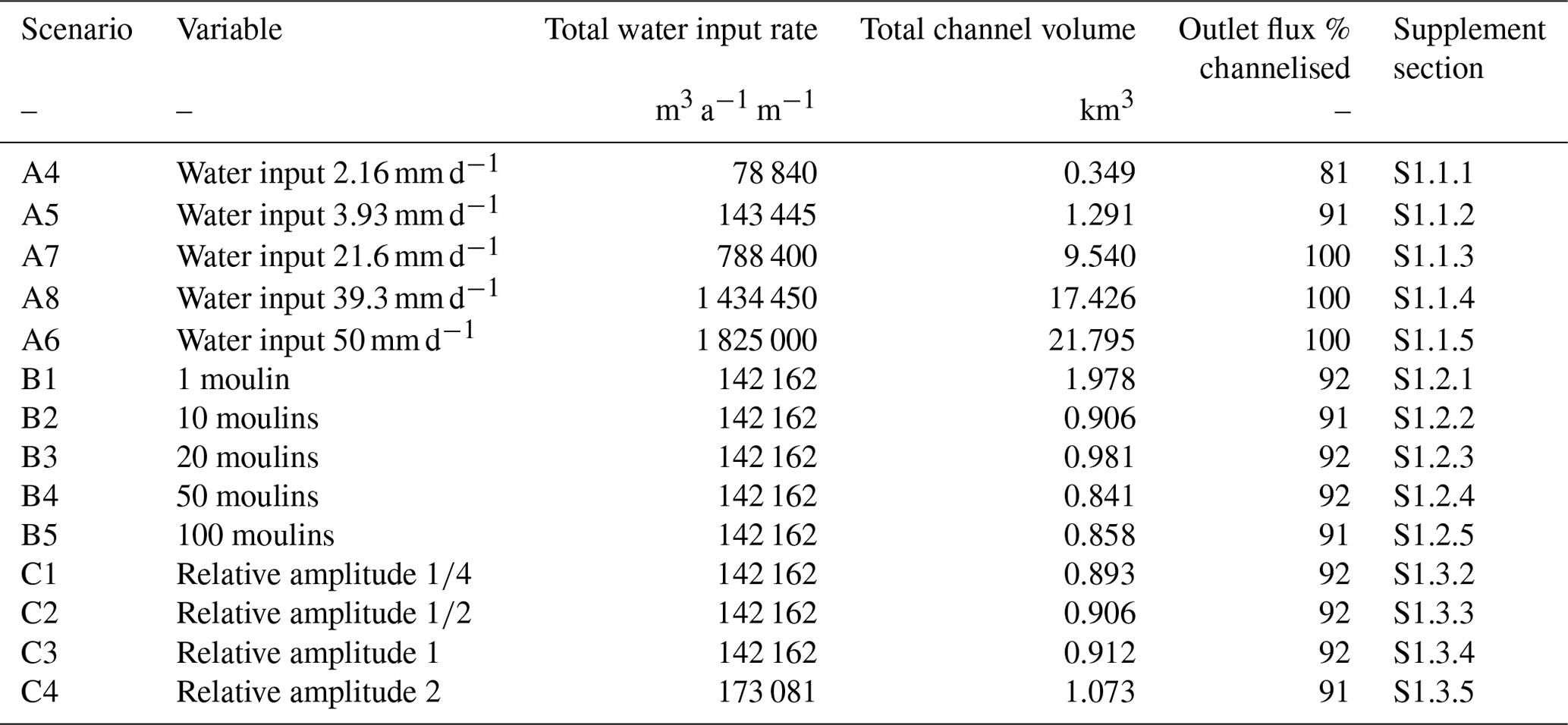
Table A2 Summary of experiment set 1 model runs. Bedrock-derived sediment values for “D” models with bedrock detritus tracking are higher; these values indicate the total erosion-derived component regardless of sediment recycling.

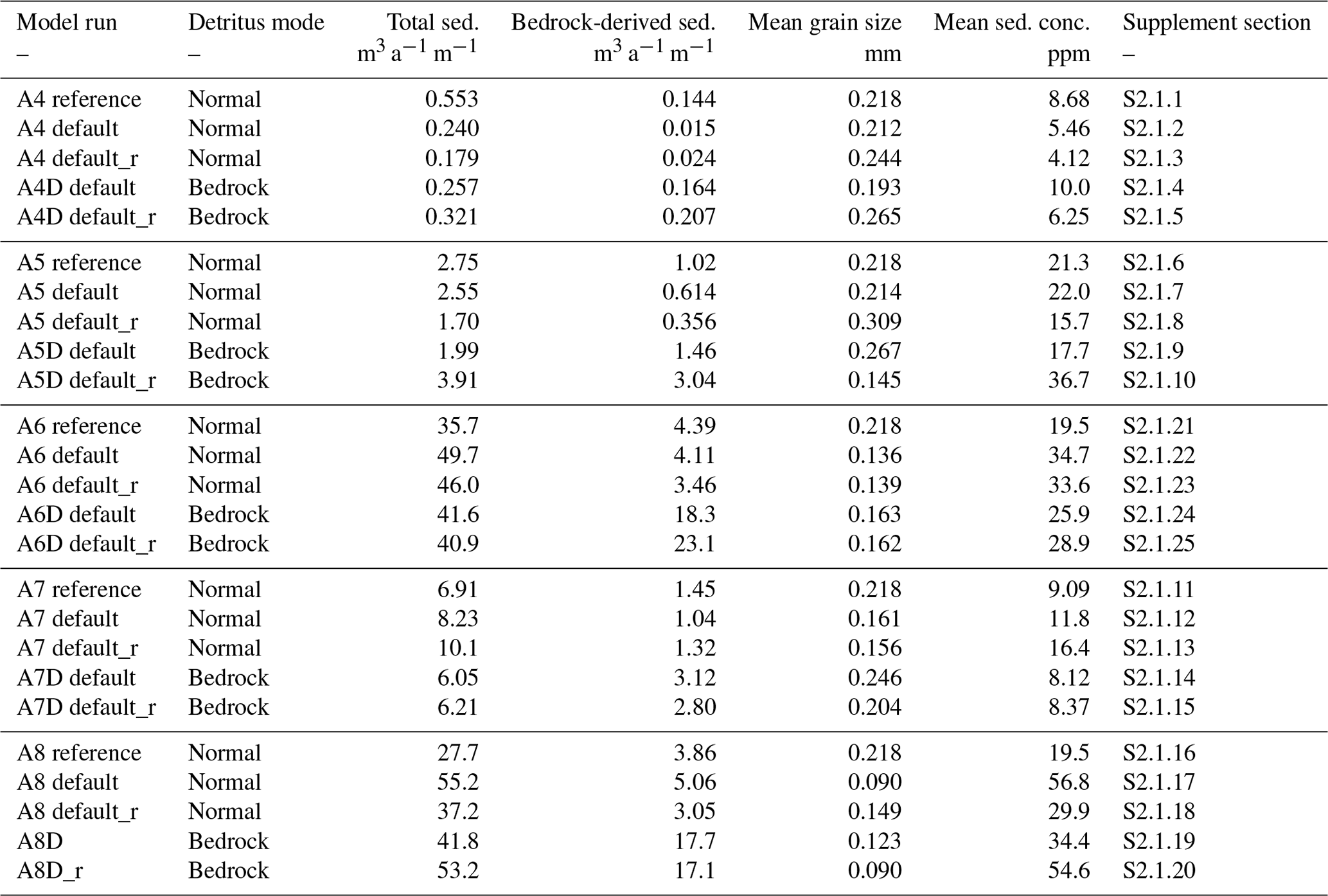
Table A3 Summary of experiment set 2 model runs, all with model scenario A5.

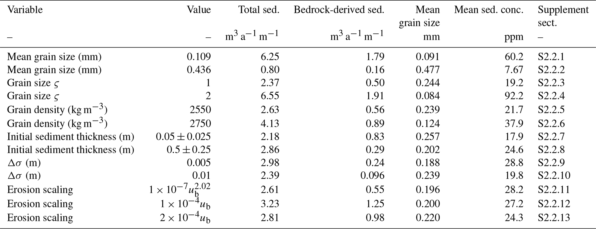
Table A4 Summary of experiment set 3 model runs. Bedrock-derived sediment values for “D” models indicate the total erosion-derived component regardless of sediment recycling.

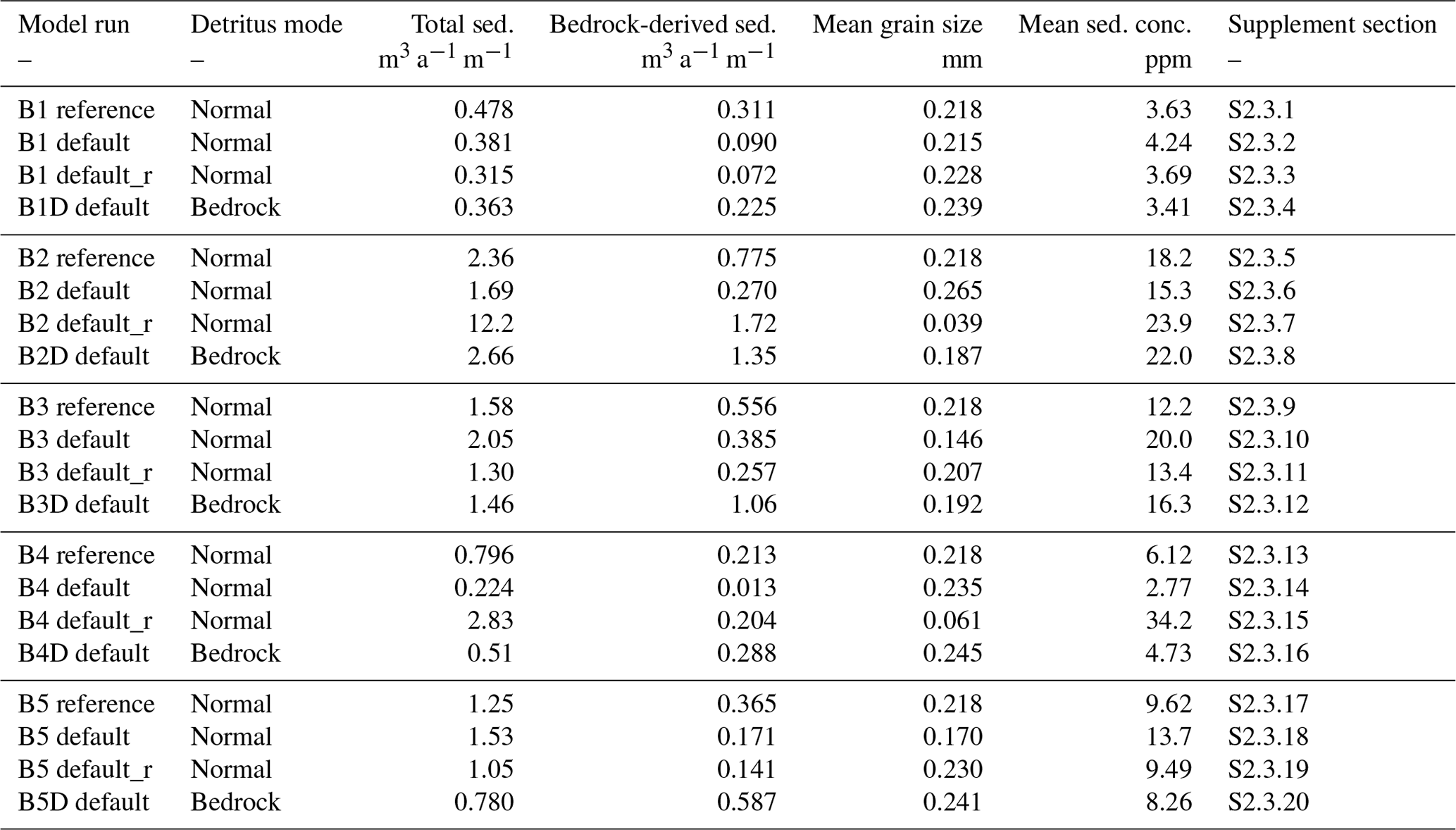
Table A5 Summary of experiment set 4 model runs. Bedrock-derived sediment values for “D” models indicate the total erosion-derived component regardless of sediment recycling.