Monthly velocity and seasonal variations of the Mont Blanc glaciers derived from Sentinel-2 between 2016 and 2024

We investigated the temporal variability of the surface velocity of 30 glaciers in the Mont Blanc massif (European Alps). We calculated the monthly velocity between 2016 and 2024 using digital image correlation of Sentinel-2 optical imagery. The main objectives of the study were (i) to characterize the variability of the velocity fields of such glaciers (referring to both their temporal seasonal and inter-annual and spatial variations) and (ii) to investigate relationships between the morphology of glaciers and their kinematics. We measured monthly velocities varying from 12.7 to 487.4 m yr⁻¹. We observed an overall decrease in the velocity between 2016 and 2019 and an unexpected rise in 2020–2022, which are especially visible in most glaciers on the southern side of the massif. Considering the whole period, half of the glaciers showed positive acceleration, which reached values > 4 m yr⁻² in three glaciers. In general, the trend's absolute value in the cold season is higher in the case of positive acceleration and lower in the case of negative acceleration. We found that smaller glaciers have a more pronounced seasonality, with winter–summer velocity differences of 50 %–100 %. Finally, in 2016, 2018, and 2022, we observed an exceptionally high winter–summer velocity difference in the 0.3 km² wide Charpoua Glacier, when summer velocities increased by 1 order of magnitude.

1 Introduction

Glacier flow has been one of the early drivers of glaciological interest and research since it was first studied. Its understanding and modelling evolved via the observations and findings of Somigliana (1938) in the early 1900s, Glen's laboratory experiments (Glen, 1952), and the interpretations of Nye (1952), to cite just a few, and these have explained how the two main mechanisms of glacier flow rely on ice deformation and basal sliding. However, the motion of Alpine glaciers is largely related to basal sliding (Willis, 1995). Because continuous monitoring of sliding velocities in the field is extremely difficult and rarely achieved (Vincent and Moreau, 2016), measuring surface flow velocities can be a strong alternative approach. Nonetheless, the continuous monitoring of surface velocities of Alpine glaciers is complex at specific study sites, and very rarely has it been performed on a spatially distributed scale.

The flow of glaciers generally depends on a variety of physical parameters. The main physical parameter influencing ice velocity is ice thickness (Jiskoot, 2011), which is indirectly related to the glacier trend in mass balance as it determines an evolution towards an increase or decrease in glacier thickness. Other parameters that influence ice flow are glacier surface slope, ice properties (temperature, density), bedrock conditions (hard, soft, frozen, or thawed ice–bedrock contact), topography, glacier terminal area type (land, sea, ice shelf), air temperature and precipitation, and their seasonality that influences sub-glacial hydrology (Jiskoot, 2011; Humbert et al., 2005; Cuffey and Paterson, 2010; Benn and Evans, 2014; Bindschadler, 1983).

The analysis of glacier surface velocity has a wide array of applications: it is a powerful climate change indicator (Beniston et al., 2018) and also an important input datum for ice thickness models (Millan et al., 2022; Samsonov et al., 2021) and mass balance models that can approximate sea level rise contributions by glaciers (Zekollari et al., 2019). In the field of glacial hazards, it is used as an indicator for the detection of glacier surges with space-borne measurements (Kamb, 1987; Kääb et al., 2021) and accelerations that can result in glacier-related hazards using ground-based sensors (Pralong and Funk, 2006; Giordan et al., 2020). Measurements of the surface velocities of glaciers can be taken using terrestrial techniques (Dematteis et al., 2021) such as topographic measurements of stakes or fixed points on the glacier (Stocker-Waldhuber et al., 2019), Global Navigation Satellite System (GNSS) repeated or continuous surveys (Einarsson et al., 2016), digital image correlation of oblique photographs (Evans, 2000; Ahn and Box, 2010), and terrestrial radar interferometry (Luzi et al., 2007; Allstadt et al., 2015). Considering remote sensing solutions, glacier surface velocities can be measured by different aerial and space-borne sensors. In recent decades, public access to satellite optical and radar data (especially from Sentinel and Landsat constellation satellites), combined with the commercial availability of very-high-resolution (30 cm to 3 m ground resolution) optical imagery (Deilami and Hashim, 2011) and radar data (Rankl et al., 2014), has given great input for glaciological research. In particular, Sentinel-2 optical imagery is widely used in glaciological studies and has been tested in the literature on various environments (Paul et al., 2016; Millan et al., 2019). Nowadays, the automated processing of ice velocity maps with global coverage from satellite imagery is freely available online from web-based platforms such as the GoLIVE datasets (Fahnestock et al., 2016), the ITS_LIVE data portal (https://its-live.jpl.nasa.gov/, last access: 19 March 2022), or the FAU-Glacier portal (RETREAT, 2021; ice surface velocities derived from Sentinel-1, Version 1; http://retreat.geographie.uni-erlangen.de/search, last access: 14 July 2022). The availability of such datasets is very relevant globally. Still, their application to Alpine glaciers is limited due to their relatively coarse spatial resolutions – e.g. 300×300 m (GoLIVE) or 120×120 m (ITS_LIVE) – which can provide data on just a few of the largest Alpine glaciers. Moreover, for the ITS_LIVE dataset, the velocity maps are calculated at a resolution of 240 m and are statistically downscaled to 120 m, which has major limitations for small mountain glaciers. The adopted resolution is a trade-off between computational effort and the best resolution of the output that must cope with the global availability of the analysis. Limiting the processing of images at a regional scale decreases the computational effort compared to global products and makes it easier to obtain higher-resolution velocity maps that allow Alpine glaciers to be investigated (Berthier et al., 2005), even though very small glaciers (i.e. with widths < 250 m) are still difficult to analyse (Millan et al., 2019).

Recent studies using different techniques have measured spatio-temporal variations of ice velocity on large valley glaciers in an Alpine environment like Argentière (Vincent and Moreau, 2016) and Miage (Fyffe, 2012) as well as on steep glacier snouts like Planpincieux (Giordan et al., 2020), but a spatially distributed analysis at a regional scale of the variations of velocities over glaciers with different morphological characteristics is, as of today, still lacking in an Alpine environment. Millan et al. (2022) calculated the velocities of world glaciers, but they considered a specific analysis period (2017–2018) without velocity variations in time, while Rabatel et al. (2023a) made a comparison between yearly aggregated velocity maps between 2015 and 2021 over three different Alpine massifs.

Other studies focused on long-term glacier velocity records in the Mont Blanc massif at Argentière Glacier (Vincent and Moreau, 2016) and Miage Glacier (Smiraglia et al., 2000; Fyffe, 2012). At Argentière Glacier, a unique series of continuous basal sliding measurements existed from 1997 and was still active as of 2022 (Vincent et al., 2022; Nanni et al., 2020). The whole series indicates a general decrease in basal sliding velocities (Vincent and Moreau, 2016) since the end of the 1990s. This general decrease has shown a strong correlation with the negative mass balance of the glacier, which agrees with the conceptual model from Span and Kuhn (2003) in which the glacier flow variation is primarily driven by the mass balance of the accumulation area in the previous year (as it determines glacier thickness variations). Seasonal field surveys conducted at Argentière Glacier from the 1950s document a longer data series than the start of basal sliding measurements in 1997, and an increase in surface velocities was measured during a period of positive mass balances in the early 1980s (Vincent and Moreau, 2016). The same trend was highlighted by Span and Kuhn (2003) for at least six other glaciers: Saint Sorlin in France; Gietro and Corbassiere in Switzerland; and Pasterze, Vernagtferner, and Odenwinkelkees in Austria. At Miage Glacier, surface velocities have historically been measured by different authors (Diolaiuti et al., 2005; Smiraglia et al., 2000; Fyffe, 2012; Lesca, 1974; Pelfini et al., 2007; Deline, 2002) and have also shown a general velocity decrease in recent decades (Smiraglia et al., 2000; Fyffe, 2012). Glaciers such as Miage and Argentière reach a low altitude and have flat and little crevassed valley tongues. For this reason they have historically often been chosen for glaciological field surveys (Span and Kuhn, 2003). Therefore, knowledge of Alpine glacier kinematics is generally mostly related to this type of glacier, which can be significantly different compared to the other glaciers analysed in this study.

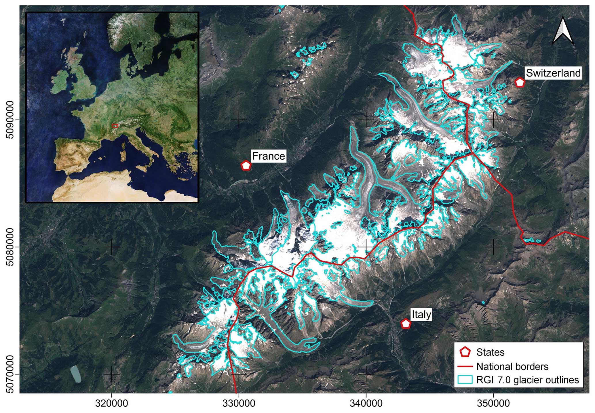
Figure 1 Study area of the Mont Blanc massif. Background: true colour image (cloud-free European mosaic in the upper-left panel) courtesy of the Copernicus Open Access Hub (https://scihub.copernicus.eu, last access: 10 September 2023).

Globally, glacier slowdown linked to a negative mass balance trend was also shown by Heid and Kääb (2012) for six different regions around the globe and for dates spanning from 1953 to 2009 in an analysis of remotely sensed optical images. Specific analysis of velocity trends and glacier mass loss showed generalized decreasing velocity trends over different regions of High-Mountain Asia between 2000 and 2017 and a strong correlation with the negative mass balance trend (Dehecq et al., 2019).

The main purposes of this study are the production of 8-year long velocity time series of the surface velocities of 30 glaciers at a massif scale (derived from Sentinel-2 optical images) and an integrated analysis of the morphological and kinematic features of such glaciers. The identification of possible trends in the velocity time series is a major objective of the present study. We observed different behaviours of surface velocity and identified a relationship between seasonality and glacier size.

2 Study area

The study area is the Mont Blanc massif. It is located in the western part of the European Alps bordering France, Italy, and Switzerland (Fig. 1) and culminates at 4809 m a.s.l. with the Mont Blanc summit, the highest peak in central Europe. Many other peaks in the Mont Blanc massif reach well above 4000 m a.s.l., and the entire area is highly frequented, with famous tourist resorts such as Courmayeur and Chamonix attracting thousands of tourists every year.

The total surface of glaciers in the Mont Blanc massif is equal to 169 km² and contains 116 glaciers, according to the Randolph Glacier Inventory (RGI 7.0) (RGI Consortium, 2023). The inventory refers to 2003 (Pfeffer et al., 2014). Forty of the glaciers are very small (covering an area of less than 0.1 km²), 47 have surfaces between 0.1 and 1 km², 16 are between 1 and 3 km², and 13 have surface areas of more than 4 km².

The geological setting and the geomorphology of the Mont Blanc massif form a high mountain range, with its main ridgeline oriented in a SW–NE direction along the French–Italian border. The valley floors flanking the massif have low altitudes – in the range of 1000–1500 m a.s.l. – resulting in steep slopes originating from the highest peaks with large vertical altitudinal differences. The meteo-climatic local conditions on the massif are of a continental type, but orographic effects on the predominant incoming weather fronts produce higher precipitation compared to the nearby regions (Gottardi et al., 2012).

Argentière Glacier is the only one with regular mass balance measurements in the World Glacier Monitoring Service (WGMS) Reference Glaciers dataset for the Mont Blanc massif (Zemp et al., 2009). It has shown a generally negative mass balance trend since the early 1990s (Vincent and Moreau, 2016), in line with mass balances of other Alpine glaciers and glaciers from other mountain ranges across the globe. Geodetic mass balance measurements of Thoula Glacier, a small glacier on the border between France and Italy at altitudes between 2900 and 3300 m a.s.l., represent well the local meteo-climatic conditions that result in slightly less negative mass balance trends compared to other glaciers in the Alps (Zemp et al., 2021, 2020; Mondardini et al., 2021).

A more spatially distributed analysis of mass balances in the Mont Blanc region has also been outlined in the literature by employing geodetic mass balances of the whole Mont Blanc massif and stereo satellite imagery from the Pléiades and Spot satellite constellations (Berthier et al., 2014; Beraud et al., 2023). The trend outlined by Berthier et al. (2023) at the massif scale reflects data trends comparable to the glaciological mass balances of WGMS reference glaciers in the Alps. Glaciers at lower altitudes show larger ice volume losses and subsequent substantial glacier front retreats (Paul et al., 2020), while glaciers at higher altitudes suffer less acute volume loss and shrinkage. Large differences in the glacier frontal position, especially for the lower-altitude terminating glaciers, can be assessed well by the difference in the terminus position in recent satellite imagery compared to the position outlined in RGI 7.0.

3 Materials and methods

3.1 General workflow

In this paper, we analysed the Copernicus ESA Sentinel-2 optical satellite imagery dataset available for the study area. In addition, we used Pléiades stereo digital elevation models (DEMs) to retrieve morphometric data of glaciers and publicly available modelled ice thickness data from Millan et al. (2022). We used digital image correlation (also known as feature tracking) to produce monthly averaged and multi-year averaged velocity maps to investigate variations of glacier surface velocity in time and space over the selected glaciers. We can hereby summarize the workflow that was used (Fig. 2).

The input data are a DEM of the study area, the RGI glacier outlines, the modelled glacier thickness, and the stack of Sentinel-2 images in the reference period. The input DEM is used to obtain morphometric data of the glacier, while the RGI glacier outlines and the selected satellite imagery are used to choose suitable glaciers for surface glacier velocity analysis. After the glacier selection, we updated the RGI glacier outlines according to the current glacier extensions. The selected imagery is processed with digital image correlation to obtain glacier velocities. The glacier flowlines of the RGI are then used, together with the updated glacier outlines and the mapped equilibrium line altitudes (ELAs), to identify sampling areas to extract velocity time series. The ELAs are manually digitized each year through analysis of the Sentinel-2 imagery. Subsequently, the time series are analysed to identify general trends, seasonal patterns, or particular kinematic behaviours. Finally, the velocity dataset is analysed in relation to the morphological characteristics (in particular their sizes) of the glaciers.

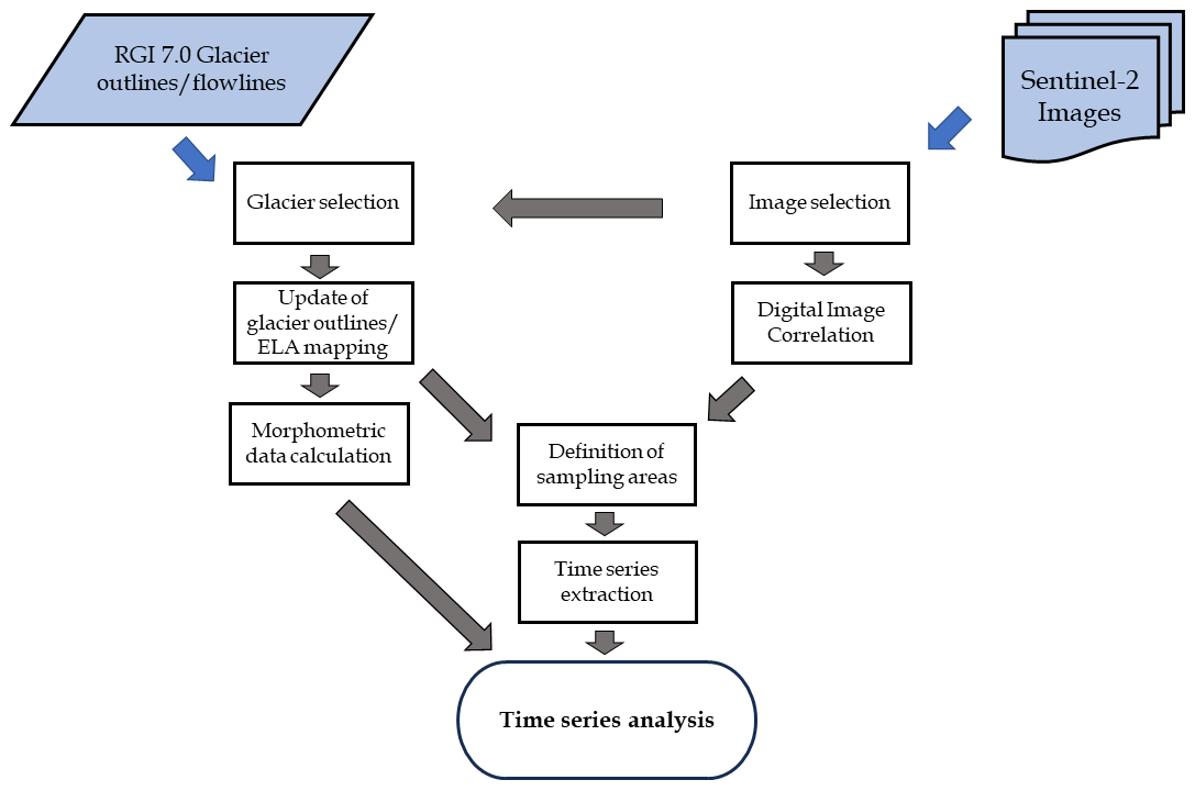
Figure 2 Workflow of the present study. The input datasets are indicated in light blue, while the processing steps are indicated in white.

3.2 Sentinel-2 optical satellite imagery

We adopted Sentinel-2 optical images acquired between February 2016 and February 2024. We chose to start the analysis in 2016 because it was the first full year of acquisition by the satellite. Based on different publications (Kääb et al., 2016; Millan et al., 2019), the geometric misregistration of Sentinel-2 can show up to 1.5 px offsets in the horizontal plane even if it can usually be closer to a value of 0.5 px, which corresponds to the absolute geolocation specification by the ESA. Therefore, an image co-registration process or a correction of stable ground shifts is normally needed for multi-temporal analyses.

To select the images, we defined the presented approach. (i) To maximize the geometric and georeferencing precision, we adopted images acquired from the same orbit and tile (GRANULE T32TLR, relative orbit 108). (ii) To reduce the impact of clouds, we carried out a visual check of all images with a cloud cover percentage lower than 80 % (as detected by the Copernicus cloud cover estimation algorithm) on the whole tile, which totalled 323 (150 from Sentinel-2B and 173 from Sentinel-2A). From this dataset, we extracted a subset of 123 cloud-free images of the selected glacier areas via visual inspection of the individual images. We adopted this manual selection to maximize the quality of the images; in the case of the Mont Blanc massif (like in most mountainous areas worldwide), the local distribution of clouds can be extremely variable. In many cases, this can contribute a considerable cloud percentage, even though high-altitude areas may still be cloud-free.

The number of suitable images available per year varies from 10 to 20, with a yearly mean of 15 images in the following distribution: 2016: 10; 2017: 18; 2018: 11; 2019: 14; 2020: 13; 2021: 16; 2022: 20; 2023: 19; 2024: 2. The year 2016 and partially the year 2017 are influenced by the lack of Sentinel-2B images, which were launched on 7 March 2017.

To apply image correlation, we used the near-infrared band B08 at the processing level L1C, as suggested by previous studies (Kääb et al., 2016).

3.3 Glacier selection

To minimize the presence of noisy and unreliable velocity data, we made a selection of glaciers from the RGI 7.0 dataset. In particular, we did not include in our study (a) glaciers with an area of < 0.1 km², as these would be too small for reliable extraction of velocity maps with 10 m resolution optical satellite imagery (Millan et al., 2019); (b) glaciers showing strong variations of cast shadows; or (c) glaciers that lack surface features to be tracked (e.g. ice caps).

Point (b) was selected by creating a stack of images acquired between October and March, when cast shadows appear on satellite imagery, especially on north-facing slopes. Subsequently, we manually identified glaciers that are subject to large variations of shadow on their surfaces. We used the scene classification map (SCL) class 11 (cast shadows), available in processing level L2A of the Sentinel-2 images. However, since shadows on glaciers may often be misclassified, we conducted a manual check to correct potential errors. Point (c) was selected manually by choosing glaciers that show very even surfaces on Sentinel-2 images. This is normally noted in ice caps at higher altitudes or in flat valley tongues.

The glacier selection process identified 30 glaciers with a total glacierized surface (in 2018) of 85.8 km². Compared to the total glacierized surface of the massif from RGI 7.0, this represents 50.8 % of the total of 169 km² and 25.9 % in terms of the number of glaciers. This rises to 39.5 % if we consider the subset of 76 glaciers with a glacierized surface of more than 0.1 km². The selected glaciers are highlighted in Fig. 3 and listed in Table 1. Two of the selected glaciers are located in Switzerland, 10 in France, and 18 in Italy. This distribution is mainly due to a small portion of the massif being located in Switzerland and the presence of more fragmented glacierized bodies on the Italian side. Seven of the 30 glaciers have been mapped as sub-areas compared to RGI 7.0 individual glacier bodies. A brief description of all the glaciers we analysed is found in Sect. S1.1 in the Supplement to give the location and geomorphological setting of the glaciers as well as to highlight when a single glacier complex from RGI 7.0 was divided into independent glacial bodies because of very distinct kinematic behaviour.

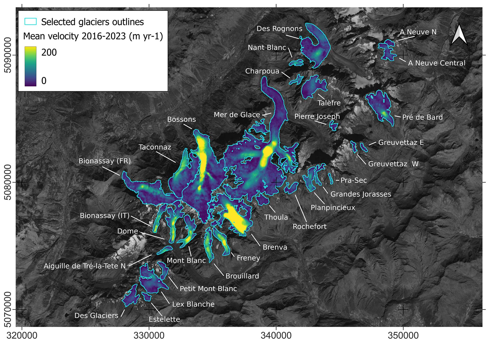
Figure 3 Surface glacier velocity map averaged in the 2016–2024 period. Selected glaciers for specific analyses are outlined in cyan. Background: Sentinel-2 image (B08 band), courtesy of the Copernicus Open Access Hub (https://scihub.copernicus.eu, last access: 10 September 2023).

3.4 Glacier outline delineation and morphometric data calculation

Since the RGI 7.0 glacier outlines refer to 2003, we updated them to fit the present glacier extensions and manually outlined them from Sentinel-2 imagery. We selected a cloud-free scene acquired on 28 August 2018 that represents the conditions of the glaciers in the study period well; True Color Image was used for this purpose. The main morphometric data that were determined for each glacier are summarized in Table 1. In some cases, a morphological indication that some parts of the glaciers could be considered independently of others and divided into individual kinematic domains was considered (Paul et al., 2022; Zemp et al., 2021). As the velocity maps confirmed distinct behaviours of some glacier parts, those glaciers were divided and mapped accordingly. The main examples are the tributary glaciers of the larger Miage Glacier complex, which all have distinct kinematic behaviour well-differentiated from the slow-moving, debris-covered main central valley tongue. Another example is the Talèfre Glacier, where, over the past 20 years, the western part of the glacier has become independent of the eastern part.

The determination of morphometric data of sample glaciers was performed using altitudinal data from a 2 m resolution DEM obtained by processing Pléiades stereo pairs acquired in August 2018 (Berthier et al., 2014), while the mean glacier thicknesses were extrapolated from globally modelled ice thickness data (Millan et al., 2022), which have an average uncertainty of 30 %.

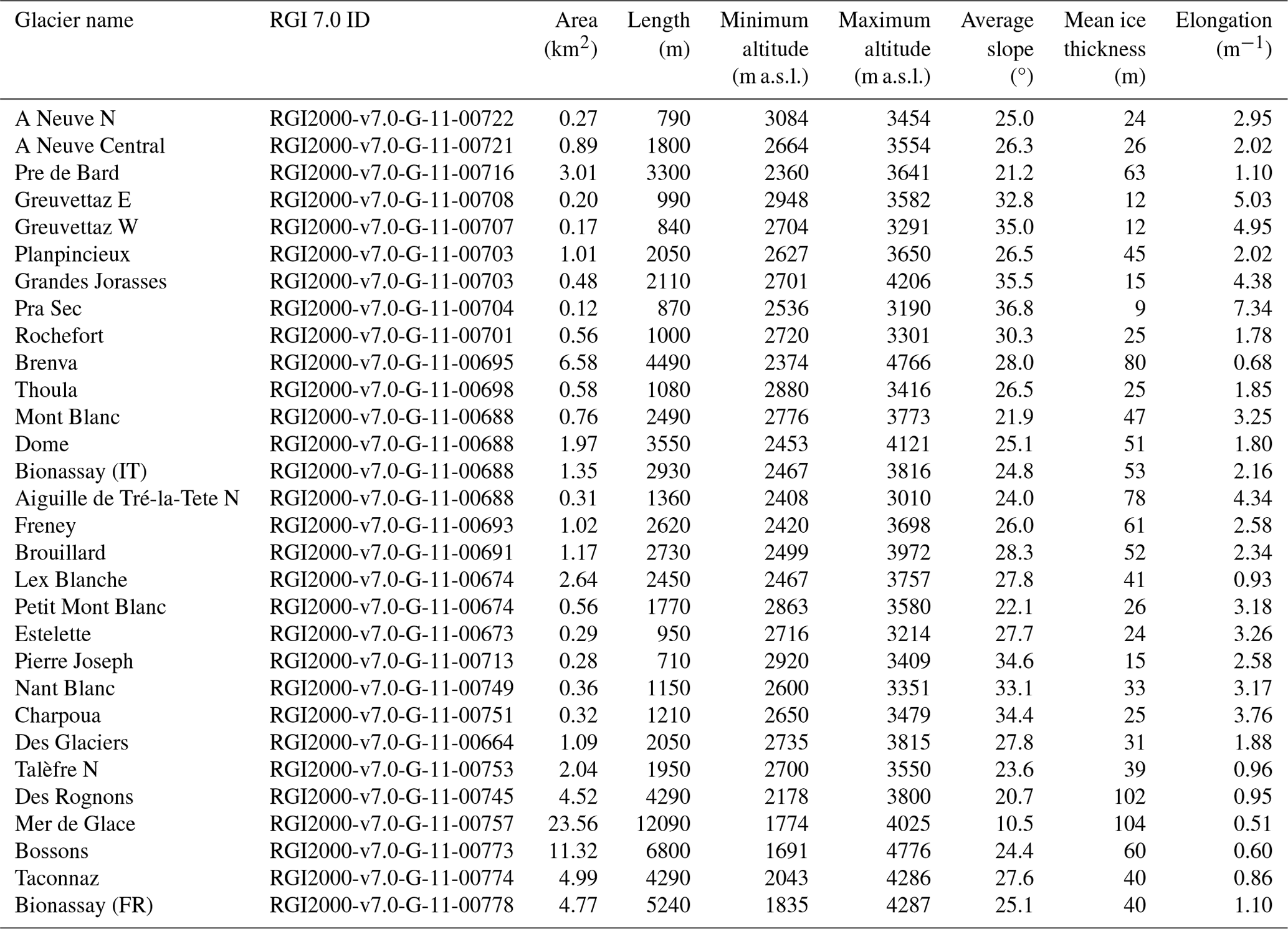
Table 1 Table with the names and RGI identification codes of the glaciers selected for analysis in the present study, together with the main morphometric parameters. The elongation is the glacier length divided by its area.

3.5 Glacier surface velocity calculation

Digital image correlation is a common technique used to measure surface displacements using proximal (Evans, 2000; Ahn and Box, 2010; Schwalbe and Maas, 2017; Dematteis et al., 2024) and remotely sensed imagery (Scambos et al., 1992; Heid and Kääb, 2012; Marsy et al., 2021; Dematteis and Giordan, 2021). The processing chain performed in the present study uses the open-source Glacier Image Velocimetry (GIV) toolbox (Van Wyk De Vries and Wickert, 2021). GIV uses frequency-based correlation, can efficiently process large datasets, and has been shown to perform well on glacier surface velocity measurements at different test sites (Van Wyk De Vries and Wickert, 2021). GIV calculates stable ground shifts to correct for georeferencing errors; therefore, we created a stable ground mask composed of non-glacierized terrain surrounding the massif and fitted a two-dimensional second-degree polynomial to the residual velocities over stable ground in the x and y directions. To measure glacier surface velocities, we adopted the “multi-pass” option, which updates displacement estimates over multiple iterations, refining initial coarse chip size displacement calculations using progressively smaller chip sizes. The initial chip size is automatically defined by GIV and cannot be smaller than 32×32 px. The overlap between matching windows was 0.5. Velocities higher than 1500 m yr⁻¹ were considered unrealistic and were discarded. The velocity map resolution was set to 40 m without resampling. Finally, we smoothed the velocity maps by applying a 3×3 median filter.

To produce the time series, given a specific image, we processed the first and second subsequent images (GIV second-order time oversampling). The minimum and maximum temporal repeat cycles were 10 and 120 d, respectively. We calculated 218 image pairs, with an average temporal baseline of 35 d (Sect. S8 in the Supplement).

Subsequently, the velocities of image pairs were averaged on a monthly basis. We applied the weighted average included in GIV, where the weights are proportional to the fraction of time included in a given month over the total time gap between the image pairs. The presence of clouds or snow on the glacier surface made it impossible to extract reliable data in the following months: (i) January 2017, (ii) December 2020 and January and February 2021, and (iii) September 2021. The gaps only represent 5 months in which we did not retrieve velocity data out of the 8 years considered in the study (i.e. < 5 %). In Fig. 3, we present a velocity map with a resolution of 40 m. This was obtained by averaging all the single monthly velocity maps in the study period (2016–2024). In Fig. 4, we present an example of the obtained velocity map and the distribution of sampling areas over several chosen glaciers. All other parameters of the GIV processing were set as default parameters (Supplement Sect. S5).

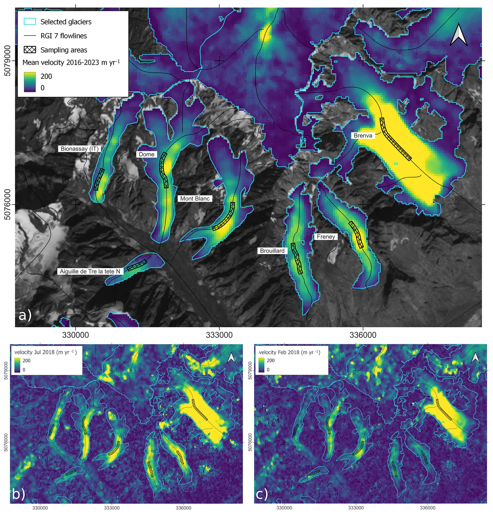
Figure 4 (a) Details of the glacier surface velocity map averaged in the 2016–2024 period and sampling areas of selected sample glaciers. Panels (b) and (c) show monthly velocity maps of July and February 2018, respectively. Sentinel-2 imagery base map (B08 band), courtesy of the Copernicus Open Access Hub (https://scihub.copernicus.eu, last access: 10 September 2023).

3.6 Velocity time series analysis

Sampling areas were identified on the velocity maps to analyse the time series of the selected glaciers. Since the surface velocities of land-terminating glaciers are expected to be highest in correspondence to the ELA (Nesje, 1992), we cropped the RGI 7.0 flowlines at the upper and lower altitudinal limits of the ELAs mapped between 2016 and 2023. Around this section of the ELA, we buffered an area of 40 m (Fig. 4). The velocity values included in the obtained polygons were averaged to produce the time series (i.e. the velocity was not calculated over all the glaciers, but only in the region of the ELA).

Subsequently, we applied quadratic locally weighted scatterplot smoothing (LOWESS) (Cappellari et al., 2013) evaluated on a rolling window of 12 months. Finally, we calculated the linear trend of the smoothed series using the Huber loss regressor (Huber, 1992). The Huber fit is robust against outliers; thus, sharp velocity fluctuations should not affect the obtained linear trends. To evaluate the statistical significance level of the fit, we consider the t statistics, i.e. the ratio between the coefficient values and their standard errors. According to its definition, the t statistics are expected to be low when the slope of the linear fit is low and/or when the slope is relatively low compared to the data variability.

We performed a principal component analysis (PCA) of the time series to investigate the overall behaviour of all the considered glaciers, and we weighted the time series according to the glacier area. PCA is a multi-variate analysis technique that allows a reduction in the dimensionality of a given dataset, increasing interpretability but minimizing information loss. This is achieved by creating new, uncorrelated variables that successively maximize the variance of the dataset (Jolliffe and Cadima, 2016).

4 Results and discussion

4.1 Distributions of monthly velocities

Overall, considering the 30 glaciers we investigated in this study, the monthly velocity values range from 30–40 m yr⁻¹, typically reached during winter months by smaller glaciers, to > 400 m yr⁻¹, typically reached in summer or late summer by faster glaciers. Brenva and Bossons glaciers attain the highest velocities. In particular, monthly extreme values vary from 11.8 ± 9.8 m yr⁻¹, reached in January 2022 by Des Glaciers Glacier, to 487.4 ± 10.8 m yr⁻¹, reached by Brenva Glacier in July 2016. The mean surface velocities averaged over the period range from 29.9 ± 10.9 m yr⁻¹ at Pierre Joseph Glacier to 375.9 ± 10.9 m yr⁻¹ at Brenva Glacier. The standard deviation of the velocity time series of single glaciers varies from 10.3 m yr⁻¹ at Pierre Joseph Glacier to 70.7 m yr⁻¹ at Charpoua Glacier. Figure 5 presents the distributions of the raw monthly velocity of the considered glaciers.

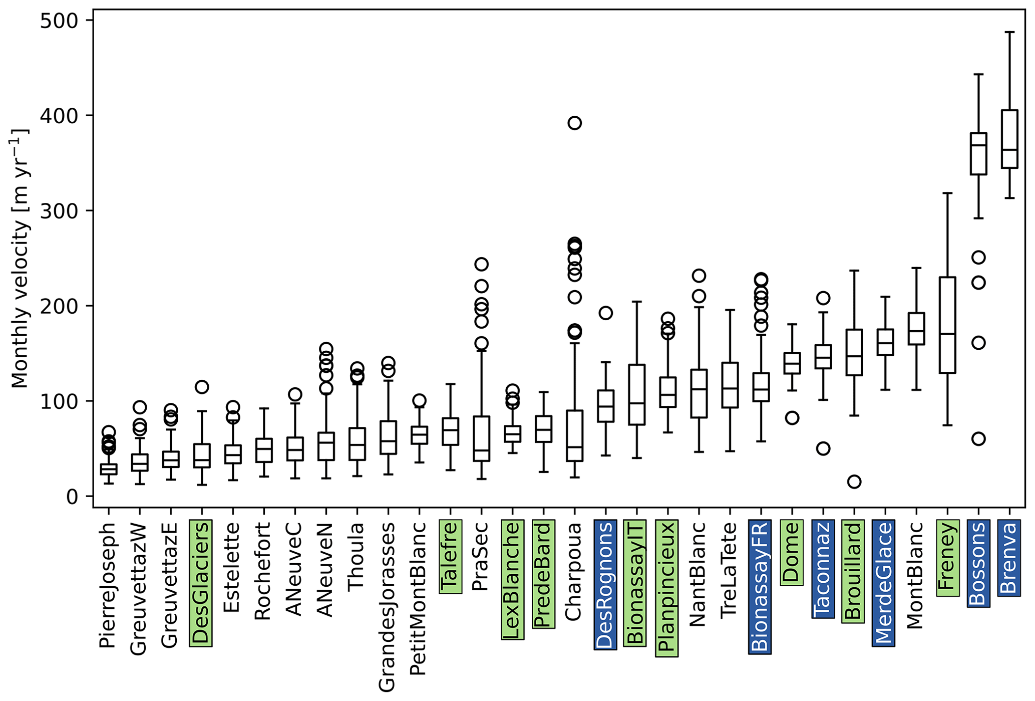
Figure 5 Boxplot showing the glaciers' raw monthly velocity distributions. Glaciers are sorted by their median velocity. The background colours of the glacier names indicate their size: white < 1 km²; green 1–4 km²; blue > 4 km². The box limits and central line represent the first, second (i.e. the median), and third quartiles, respectively. The whiskers indicate the first or third quartiles minus or plus 1.5 IQR (inter-quartile range). The white circles are outliers.

4.2 Velocity time series

Large and thick glaciers generally have high velocities: two (Brenva and Bossons) show the highest values. The velocity values remain high throughout the year (Fig. 6). Brenva displays irregular seasonality variations, while Bossons has an almost absent seasonal cycle. Their morphology is complex: for example, the slope varies considerably along their extent. In the present study, we concentrated the analyses on the middle sectors (near the ELA) of the glaciers, which are the fastest (Nesje, 1992). In the time series, the biggest glacier (Mer de Glace) appears slower because we extracted the monthly velocity over an area which does not entirely include the most active sector of Mer de Glace Glacier (i.e. the Géant icefall), where the velocity reached values > 400 m yr⁻¹.

Medium-sized glacier morphology is less homogeneous, although most are generally gentler and thicker than average. We can divide the group into two sets based on the elongation ratio. Medium-sized glaciers, which are more elongated, generally feature strong kinematic activity. Their velocity is higher than average with marked variability, and they often show a pronounced regular annual cycle, as in the cases of Bionassay (IT), Brouillard, Mont Blanc, and Freney glaciers. The second set of more “compact” glaciers shows lower mean velocities and has a minor amplitude of the seasonal variability. In particular, even though some display a regular seasonal cycle (e.g. Planpincieux, Dome, Rochefort), their velocity variability is much lower (Fig. 6).

Small glaciers show lower average velocities, but most show marked and regular seasonality. In this group, some very small glaciers (e.g. Greuvettaz W, Greuvettaz E, A Neuve N, Pierre Joseph) show a modest, irregular, or even non-detectable seasonal cycle since the velocity in winter is close to the measurement uncertainty (Fig. 6). It is worth highlighting that signals of potential velocity fluctuations could exist, but remotely sensed data are not currently suitable for analysing such small glaciers.

On the other hand, Pra Sec and Charpoua, small steep elongated glaciers, feature very low minimum velocities (between 25 and 50 m yr⁻¹) and very marked peaks during which the velocity increased by 1 order of magnitude. These high-velocity periods appear in summer or late summer, and extreme velocity changes from winter to summer can be noted. In 2016, 2018, and 2022, the summer velocity of Charpoua Glacier was exceptionally high compared to the usual velocity. Moreover, in these years, the spatial distribution of velocities varied. The highest velocities were registered towards the frontal part of the glacier. At the same time, normally they were higher in the upper sector (Fig. 7). Pra Sec Glacier displays more regular annual speedups in the period analysed: every summer it had a clear velocity peak (except in 2018) that was particularly pronounced in 2016, 2020, and 2022. In both glaciers, possible glacier advances are prevented by the steep bedrock cliff at the snout, which causes the disintegration of the glacier by repeated ice falls from the terminus (Giordan et al., 2020; Pralong and Funk, 2006).

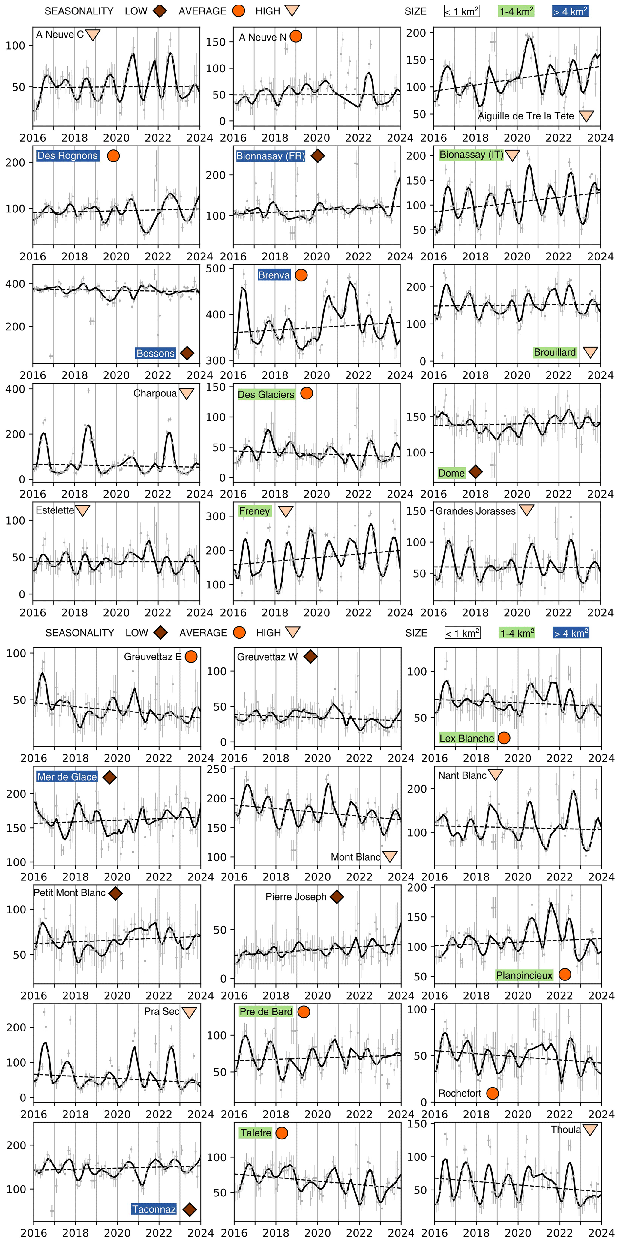
Figure 6 Time series of monthly glacier surface velocities over the 2016–2024 period. Monthly raw data and the corresponding uncertainty are depicted as grey dots and bars, while the solid black lines represent the LOWESS interpolation. The robust linear trends are represented in dashed black lines. The background colour of the glaciers' names denotes their size: white, green, and blue are for small, medium, and large glaciers, respectively. The velocity seasonality is indicated with markers: brown diamonds (low seasonality), orange circles (average seasonality), and pink rectangles (high seasonality).

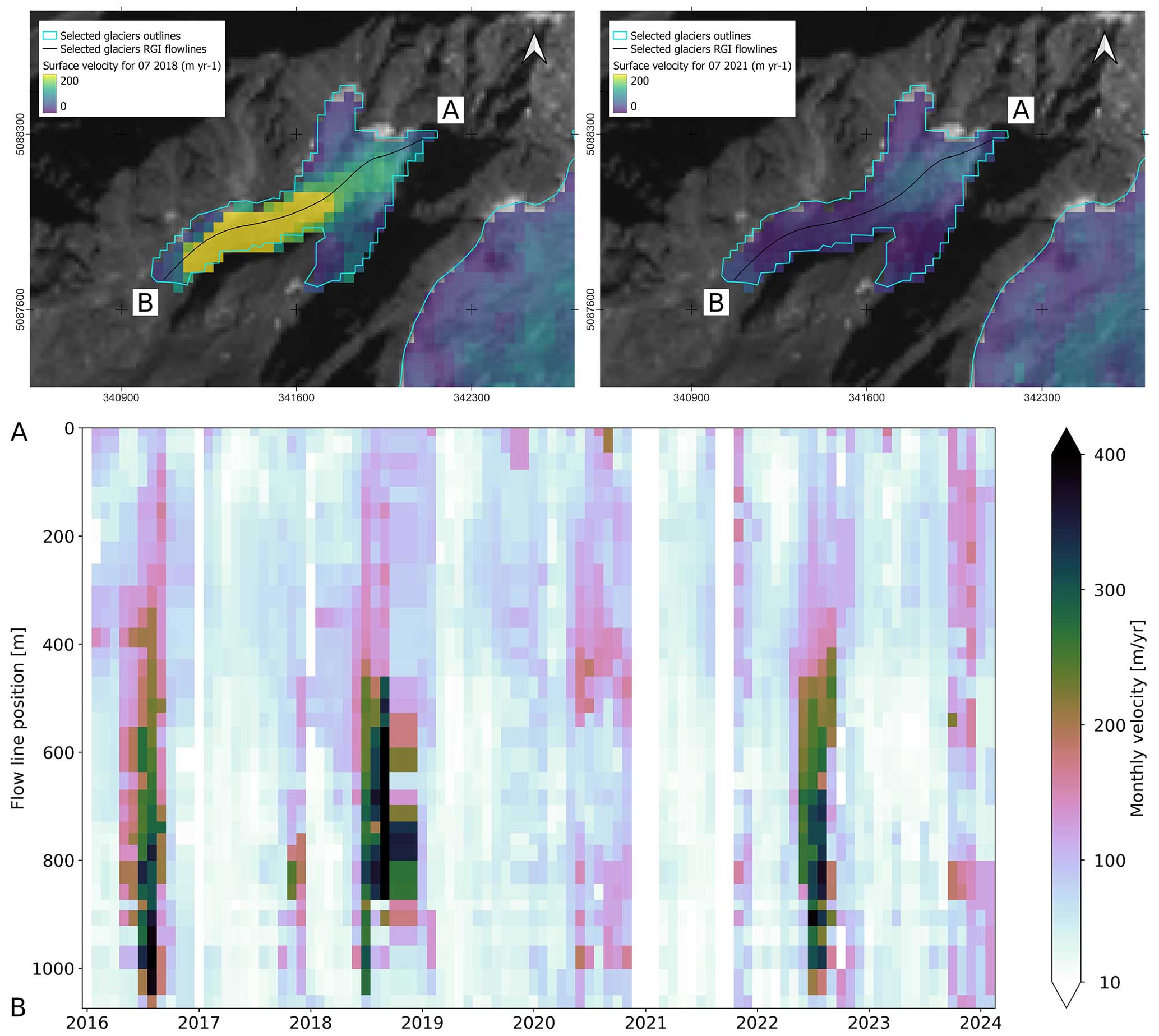
Figure 7 Charpoua Glacier monthly surface velocity maps showing the spatial variation of the velocity patterns between July 2018 (upper left) and July 2021 (upper right). The lower half shows the monthly velocity profiles along a longitudinal east–west AB profile (in black on the maps) over the study period. Sentinel-2 imagery base map (B08 band), courtesy of the Copernicus Open Access Hub (https://scihub.copernicus.eu, last access: 10 September 2023).

4.3 Inter-annual velocity variability and trend

The overall behaviour of the glacier velocity can be represented well by the PCA of the time series, weighted by the glacier area. Figure 8 shows the first principal component (PC), which explained > 50 % of the variance. In general, this analysis reflects a common trend of many time series: a first period between 2016 and 2019 showing decreasing velocities, an anomaly of higher velocities between 2020 and 2022, and a new velocity decrease in 2023 (Fig. 6). According to historical observations at Argentière and Miage glaciers, the velocity decrease from the early 2000s can be linked to continuous negative mass balances (Vincent and Moreau, 2016) of most Alpine glaciers since the 2000s (Zemp et al., 2021). The results of our study agree with this negative trend in the first part of the considered period (i.e. 2016–2019). Still, we detected a rupture in the trend and a velocity rise from 2020 to 2022 in many of the glaciers under study. An interesting remark about the geographical distribution of the trends is that the glaciers showing a clear velocity anomaly during 2020–2022 are located on the south-eastern side of the massif ridgeline along the Italian and Swiss parts of the massif (e.g. A Neuve Central, Bionassay (IT), Brenva, Planpincieux, and Lex Blanche glaciers). This might be linked to different dominant meteorological condition distributions on the two sides of the massif. A specific analysis of seasonal meteorologic data in the different areas could give more insights into this hypothesis, even though existing stations are located far from the glacier accumulation areas and could not get a specific signal present in the higher-altitude sectors.

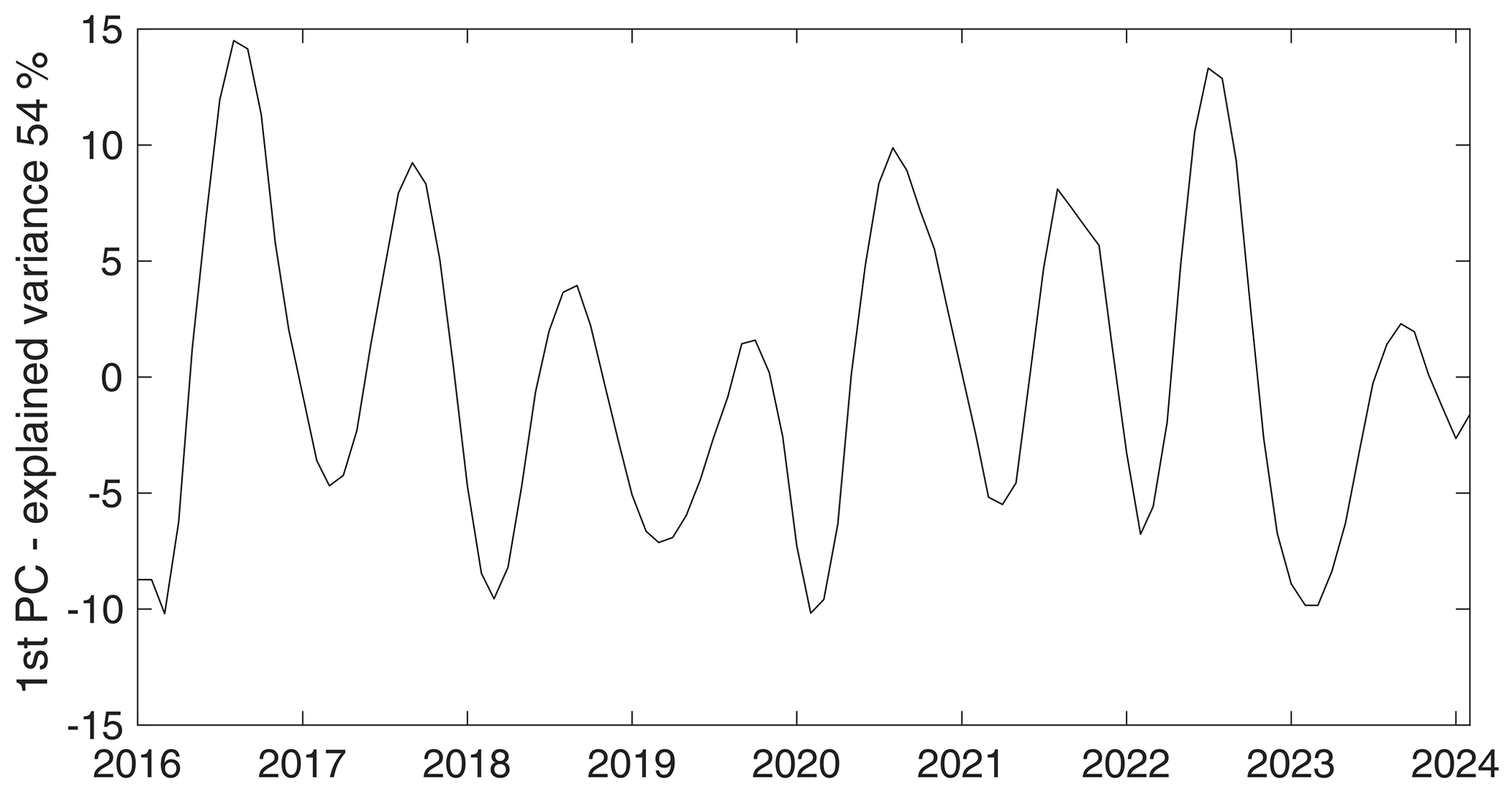
Figure 8 First principal component (PC) of the LOWESS velocity values of all the time series of glacier monthly velocity.

The glacier velocities shown in Fig. 6 have different linear trends over the full period of the study (Fig. 9). In general, the linear trends of each glacier calculated using winter, summer, or the whole year have similar behaviour (i.e. they are always negative or positive), with winter trends having higher absolute values than summer ones in the case of positive acceleration and lower absolute values in the case of negative acceleration (∼ 30 % difference on average). As expected, lower absolute linear trends (i.e. 1 m yr⁻²) have t statistics < 2. Besides, although Brenva's trend is high (2.8 m yr⁻²), its velocity is very high, thus lowering the t statistics. Most trends lie in a relatively tight cluster which crosses the domain diagonally, except for Charpoua and Planpincieux, which have dissimilar seasonal values. In the Charpoua case, this is probably related to the strong velocity fluctuations occurring only in some years in summer, while the Planpincieux positive summer trend is likely led by the anomaly of 2020–2022, which is particularly strong in this glacier. Notably, the three glaciers with the highest linear trends (i.e. Freney, Bionassay (IT), and Aiguille de Tré-la-Tete) are all located in Val Veny, on the southern side of the massif. Bionassay (IT) and Freney have a very similar morphology (Table 1): they are both medium-sized (1.3 and 1.02 km²), relatively elongated (2.2 and 2.5 m⁻¹) glaciers, with slopes of ∼ 25° and elevations between 2400 m a.s.l. and 3800 m a.s.l. Differently, Aiguille de Tré-la-Tete is a small (0.3 km²), much-elongated (4.34 m⁻¹), and low-altitude glacier (2408–3010 m a.s.l.). Aiguille de Tré-la-Tete and Bionassay (IT) are both tributaries of Miage Glacier.

An accelerating trend (5 m yr⁻² between 2015 and 2021) has recently been shown for Brenva Glacier through an analysis of remotely sensed optical images (Rabatel et al., 2023b) while detecting decelerating trends on many other glaciers of the massif. Our study showed that Brenva Glacier had an accelerating trend of 3 m yr⁻² between 2016 and 2024, which is in good agreement considering the velocity decrease shown in 2022 and 2023 (a detailed comparison between this study and Rabatel et al. (2023b) is presented in Sect. S4 in the Supplement). In addition, Rabatel et al. (2023b) observed a slight ice thickening (∼ 1 m between 2000 and 2019) in an upper sector of Brenva Glacier, which agrees with the findings of Berthier et al. (2023) between 2012 and 2021 obtained with high-resolution satellite images. They proposed three hypotheses to explain the acceleration of Brenva Glacier: (a) a glacier thickening, (b) a change in the thermal regime, and (c) a change in the sub-glacial hydrology possibly related to increased ablation in the upper reaches of the glacier.

Even though the hypothesis of glacier thickening could explain the specific case of Brenva Glacier, the glacier surface elevation change across the Mont Blanc massif has generally been negative in recent years, as evidenced by the negative mass balance of the reference glaciers in the area (Zemp et al., 2021, 2009) as well as massif-scale studies (Berthier et al., 2023). Local anomalies of positive mass balance could explain an increase in velocity, but the lack of measurements at higher altitudes does not allow us to confirm this behaviour. However, the meteorological conditions in recent years have remained approximately constant, which makes a general glacier thickening in the region unlikely (see Sect. S6 in the Supplement, “Meteorological conditions”). Localized higher-than-usual accumulation rates due to increased avalanche activity and wind accumulation could also contribute to the ice thickening (thus yielding an acceleration) but cannot be investigated at this stage. It is worth noting that the three glaciers with high winter accelerating trends in Fig. 9 (Bionassay (IT), Aiguille de Tré-la-Tete, and Freney) are near each other and located in a small part of the massif on its south-eastern side.

A change in the glaciers' thermal regime could explain accelerating trends, but it would explain long-term trends and not short-term variations such as the one highlighted in 2020–2022, as basal temperature measurements show a warming at the ice–bedrock interface on a decadal to multi-decadal timescale on the Mont Blanc massif (Vincent et al., 2007).

Variation of the hydrology of groups of glaciers is a plausible hypothesis for the explanation of accelerating trends, but it would result in stronger trends in summer than in winter, as basal sliding is enhanced over deformation during summer. Such a combination of trends is not shown by most glaciers, as highlighted in Fig. 9. Only the trends of Planpincieux and Mer de Glace glaciers could relate well to this hypothesis, showing almost no trend in winter and an accelerating trend during the summer months.

The distribution of the acceleration trend over different areas of the massif and different types of glaciers could suggest the existence of a meteo-climatic driver of the phenomenon, even though this is not evident, limiting the analysis to the period 2015–2023 (Sect. S6). A definitive answer cannot be formulated at present, and further research is necessary to understand the processes involved in this trend.

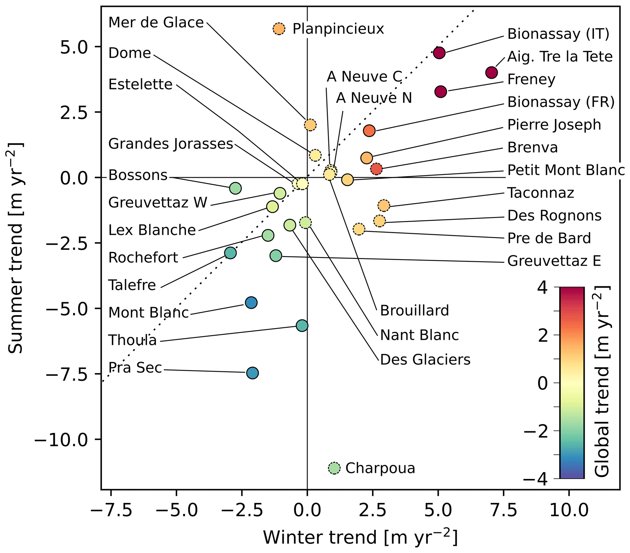
Figure 9 Linear trends of the glacier monthly velocity. The x and y axes refer to the trends calculated using winter (from November to April) and summer (from June to September) months, respectively. The colours indicate the global trend. The glaciers with linear trends with t statistics < 2 have markers with dashed edge lines.

4.4 Relationship between glacier size, velocity, and seasonal behaviour

We examined the relationship between glacier size, seasonal velocity behaviour, and monthly velocity distribution. To this end, we divided the glaciers into three classes for each feature. Concerning the size, we considered very small glaciers with an area of < 1 km², according to Bahr and Radić (2012), while medium and large glaciers have areas between 1 and 4 km² and > 4 km², respectively. Concerning the velocity distribution, we observed that, besides Brenva and Bossons, which have much higher velocities compared to the rest of the glaciers, a group of 16 glaciers has a 75th percentile of monthly velocity < 100 m yr⁻¹ (from Pierre Joseph to Charpoua in Fig. 5). Finally, 12 glaciers have their 25th and 75th percentiles between ∼ 100 and ∼ 200 m yr⁻¹ (from Des Rognons to Freney in Fig. 5).

Concerning the seasonal velocity behaviour, we analysed the raw time series (Fig. 6) and the LOWESS smoothed time series normalized by their median value (Fig. S6 in the Supplement). Glaciers such as Freney, Brouillard, and Bionassay (IT) show evident and regular seasonal behaviour and large winter–summer differences; in these cases, summer velocities (occurring between July and October) are 50 % to 100 % higher than winter ones (occurring between January and April). Another group of glaciers has smaller winter–summer differences or pronounced but irregular variability (e.g. Planpincieux, Pre de Bard, Talèfre). A third group does not show evident or regular seasonal behaviour (e.g. Taconnaz, Mer de Glace, Pierre Joseph), with winter–summer differences below 10 %. Overall, the maximum velocity occurs in August–September, while the annual minimum is reached in March (Fig. 8).

The double-entry heatmaps are presented in Fig. 10 and show a tendency for the smaller glaciers to have more pronounced seasonality, while the larger glaciers show a more homogeneous velocity throughout the year. Since the glacier area is strongly correlated with its thickness (Cuffey and Paterson, 2010), a possible cause of this phenomenon could be enhanced basal sliding during the accelerating period. In fact, a thicker glacier could be less prone to exhibiting enhanced sliding because of the larger mass to be uplifted by positive basal water pressures. In contrast, shallower glaciers could more easily benefit from enhanced sliding by pressure build-up at the ice–bedrock interface through increasing inputs in the hydrological sub-glacial drainage network. Moreover, in winter, the bases of thin glaciers could freeze, thus preventing the sliding and determining lower winter velocities, causing even larger summer–winter velocity differences.

On the other hand, as expected, larger (and thicker) glaciers tend to be faster than smaller ones.

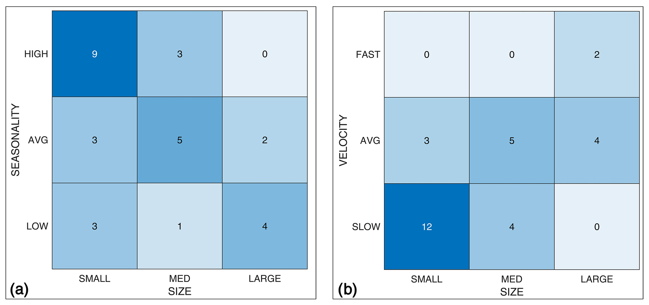
Figure 10 Glacier classification according to size (small: < 1 km²; medium: 1–4 km²; large: > 4 km²) and (a) seasonal velocity behaviour (qualitatively estimated) and (b) median velocity (slow: < 100 m yr⁻¹; average: 100–300 m yr⁻¹; fast: > 300 m yr⁻¹). The digits within the grid tiles indicate the number of glaciers belonging to each group.

4.5 Uncertainty analysis

To estimate the quality of our data, we performed two investigations. First, following the method proposed by Millan et al. (2019), we calculated the median absolute deviation of the velocity obtained on stable terrain for each monthly datum. In these areas, we applied an outliers spatial filter to the velocity maps according to Rabatel et al. (2023a). The median value of the monthly uncertainty was 10.9 m yr⁻¹. In their study, Millan et al. (2019) estimated the nominal precision according to the temporal baseline between the correlated images, which they found to be between 6 and 16 m yr⁻¹ for baselines of 40 and 20 d, which is the typical range of the temporal gaps between the images used in our study. Moreover, the value of 10.9 m yr⁻¹ is in close agreement with the uncertainty found by Mouginot et al. (2023), who obtained a root mean squared error of 10.5 m yr⁻¹ between glacier velocities measured over Mer de Glace and Argéntiere glaciers using image correlation of Sentinel-2 images and GNSS in situ data (https://glacioclim.osug.fr/, last access: 1 May 2023). A comparison with the data from Rabatel et al. (2023a) is proposed in the Supplement (Sect. S4, Fig. S3, and Table S1) for the glaciers of Brenva, Bionassay (FR), Bossons, and Brouillard over the time span that overlaps the two studies (from February 2016 to December 2021), which shows high agreement between the two studies.

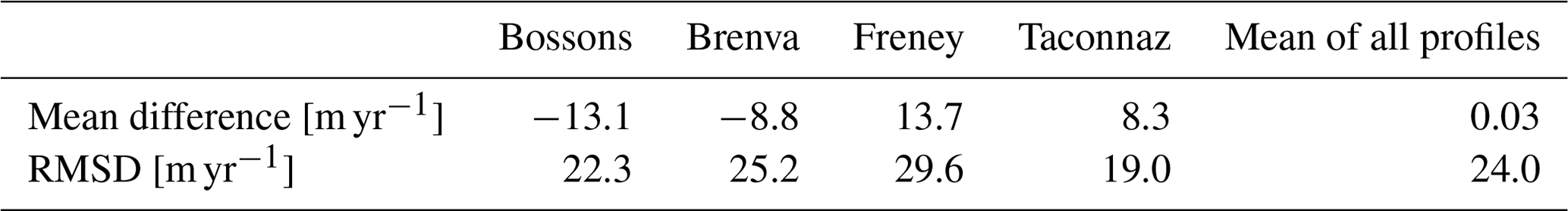
Second, we considered the glacier velocity from Millan et al. (2019), who published mean annual velocity in the period 2017–2018 on a 50×50 m regular grid. They adopted normalized cross-correlation and chip size refinement (initial size of 16×16 px). They estimated an overall uncertainty of glacier surface velocity time series of ∼ 12 m yr⁻¹ over the Mont Blanc glaciers and, specifically at Brenva and Bosson glaciers, an uncertainty of 15–20 m yr⁻¹. We compared these data and ours along four glacier longitudinal central lines (i.e. in Bossons, Brenva, Freney, and Taconnaz), obtaining good agreement (Fig. 11). The largest differences (> 50 m yr⁻¹) were found in a specific sector of Taconnaz Glacier (Fig. 11d), where the ice flux is highly channelized in a narrow passage. There, the data of Millan et al. (2019) show a large velocity decrease that seems unlikely considering the site's geometry. Our data show a similar but less pronounced velocity decrease. However, the velocity profiles are similar elsewhere. On average, the surface velocities we obtained are slightly higher, with a mean difference of 0.03 m yr⁻¹ and a root mean squared deviation (RMSD) of 24.0 m yr⁻¹ (Table 2). The slightly higher RMSD compared to the expected uncertainty could be because the error over glacierized areas is probably larger than in ice-free zones because the surface texture is different and changes (e.g. snow precipitation, surface melt, or glacier movement) occur more rapidly, thereby causing more decorrelation (Millan et al., 2019).

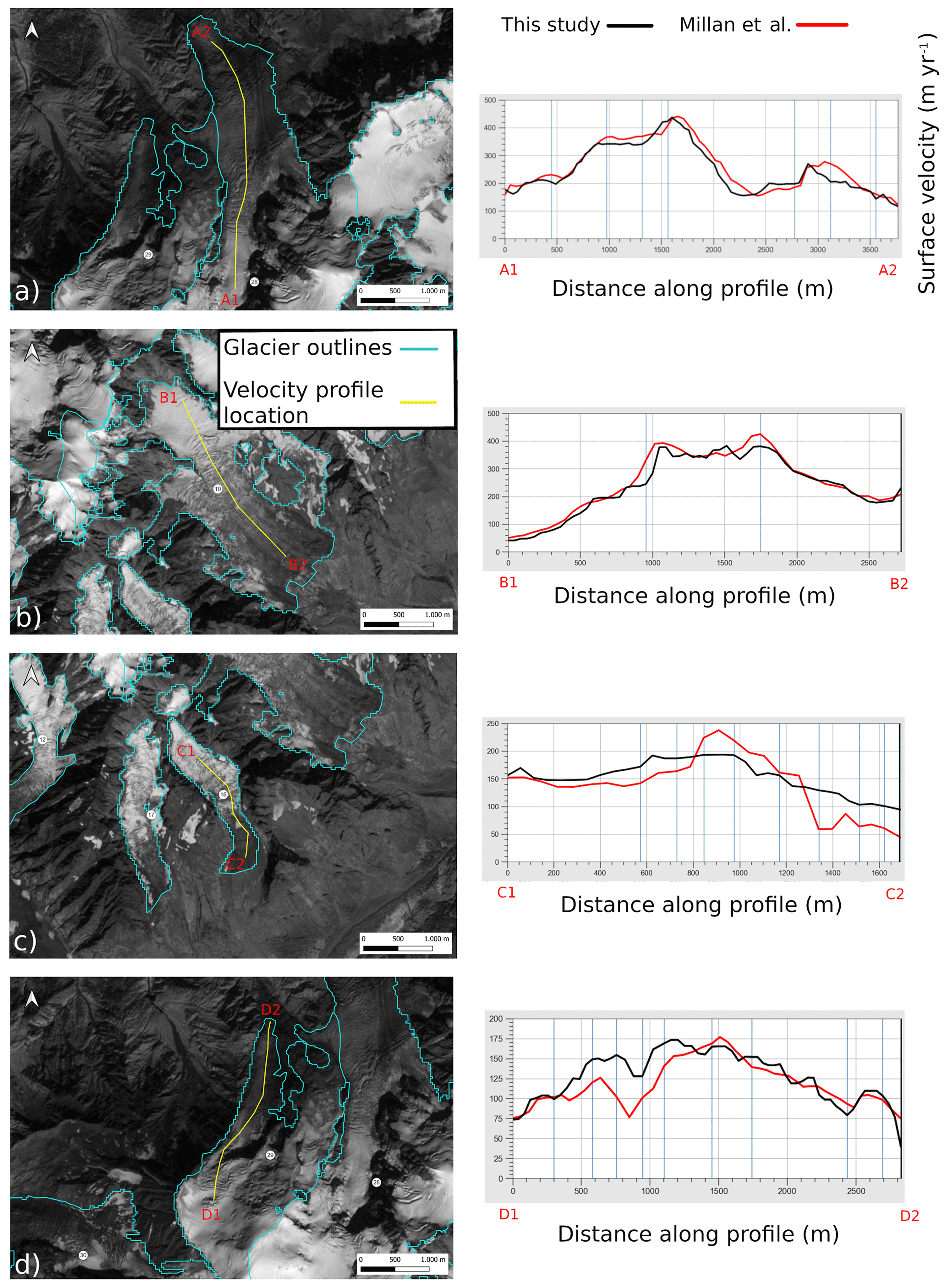
Figure 11 Comparison of velocity profiles from Millan et al. (2022) (red) and from this study (black) at (a) Bossons Glacier, (b) Brenva Glacier, (c) Freney Glacier, and (d) Taconnaz Glacier. The velocity profiles are represented in yellow on the maps on the left, and the velocity profiles go from the upper to lower altitudes. Sentinel-2 image base map (B08 band), courtesy of the Copernicus Open Access Hub (https://scihub.copernicus.eu, last access: 10 September 2023).

Table 2 Mean difference and root mean squared deviation (RMSD) between this study and Millan et al. (2022) along velocity longitudinal profiles.

4.6 Uses and limits of the proposed methodology

The methodology presented in this study allows the detection of monthly changes in glacier velocity, which can be precursors of ice avalanches (Pralong et al., 2005; Faillettaz et al., 2008; Giordan et al., 2020). For example, ice avalanches from Pra Sec Glacier occurred in 2020 (Forestry Service of Aosta Valley). In our study, we observed high velocities in 2020, which could have led to the break-off. At Charpoua Glacier, an ice avalanche of 45 000 ± 15 000 m³ occurred in 2018 (Lehmann, 2018 – https://news.unil.ch/display/1536777918113, last access: 11 October 2023), when we measured velocities > 200 m yr⁻¹ that were much higher than usual.

In this framework, measuring and knowing the typical velocity fluctuations of specific glaciers under stable conditions would be very relevant. This could allow an assessment of the extent to which a suspect acceleration may be anomalous and potentially destabilizing, bearing in mind that high-rate monitoring is essential for detecting glacial instabilities since the expected sharp increase in velocity in the weeks before the failure (Pralong and Funk, 2006) could be barely detectable by remote sensing (e.g. due to scarce visibility, image decorrelation, or low resolution).

Limits of the methodology presented in this study should also be considered: glaciers moving at slow rates can be surveyed using temporal baselines of 1 year (Millan et al., 2019; Mouginot et al., 2023), but this implies losing the ability to catch short-term velocity fluctuations, like those observed at Charpoua and Pra Sec glaciers. Another known issue pertains to the lack of features of the glacier surface that makes it impossible to track movements using optical imagery. Satellite optical imagery is limited and can be strongly influenced by the presence of clouds that could yield extensive periods without data acquisition, even though, in the present study, we only had 4 out of 96 months with no data. Anomalies due to image decorrelation for the presence of shadows, snow, or morphological surface modifications can occur, and an expert-based visual check may be required to discriminate between anomalous velocities.

5 Conclusions

We produced ice velocity maps and time series of 30 glaciers of the Mont Blanc massif during the period 2016–2024. The proposed results are different compared to the existing publicly available automatically processed velocity datasets that have a coarse resolution (i.e. > 100 m) and that cannot correctly detect the kinematics of most Alpine glaciers due to their small sizes. Therefore, specific processing and studies are needed to characterize the surface kinematics of Alpine glaciers. In our study, we used Sentinel-2 imagery due to its free availability, good ground resolution, and high revisit time in the study area to obtain monthly surface velocity time series. In addition, we proposed a classification of different groups of glaciers based on their morpho-kinematic features. We also observed a significant acceleration trend in many of the studied glaciers in the last years (2020–2022), but the causes are still poorly understood.

From a methodological point of view, the proposed approach can be very useful for processing and analysing available satellite images of other massifs in the Alps and other parts of the world. This approach could stimulate innovative research on high-resolution spatio-temporal variations of velocities in Alpine glaciers and, especially, on understanding the variations in the motion of mountain glaciers. A large research question remains open and deals with understanding and measuring the drivers of change in the motion of Alpine glaciers. This implies the complex acquisition of data related to the possible drivers of the variations, such as mass balances, water inputs, and temporal variations in the sub-glacial hydrology of individual glaciers. However, to delve further into these investigations, velocity databases at higher spatial and temporal resolutions, such as those presented in this study, are needed to build future research on the topic.