the Creative Commons Attribution 4.0 License.
the Creative Commons Attribution 4.0 License.
 | 25 Jul 2024
Spectral induced polarization imaging to monitor seasonal and annual dynamics of frozen ground at a mountain permafrost site in the Italian Alps
Theresa Maierhofer
Adrian Flores Orozco
Nathalie Roser
Jonas K. Limbrock
Christin Hilbich
Clemens Moser
Andreas Kemna
Elisabetta Drigo
Umberto Morra di Cella
Christian Hauck
We investigate the application of spectral induced polarization (SIP) monitoring to understand seasonal and annual variations in the freeze–thaw processes in permafrost by examining the frequency dependence of subsurface electrical properties. We installed a permanent SIP monitoring profile at a high-mountain permafrost site in the Italian Alps in 2019 and collected SIP data in the frequency range between 0.1–75 Hz over 3 years. The SIP imaging results were interpreted in conjunction with complementary seismic and borehole data sets. In particular, we investigated the phase frequency effect (ϕFE), i.e., the change in the resistivity phase with frequency. We observe that this parameter (ϕFE) is strongly sensitive to temperature changes and might be used as a proxy to delineate spatial and temporal changes in the ice content in the subsurface, providing information not accessible through electrical resistivity tomography (ERT) or single-frequency IP measurements. Temporal changes in ϕFE are validated through laboratory SIP measurements on samples from the site in controlled freeze–thaw experiments. We demonstrate that SIP is capable of resolving temporal changes in the thermal state and the ice water ratio associated with seasonal freeze–thaw processes. We investigate the consistency between the ϕFE observed in field data and groundwater and ice content estimates derived from petrophysical modeling of ERT and seismic data.
- Article
(18189 KB) - Full-text XML
- BibTeX
- EndNote


High-mountain environments are facing a rapid increase in air temperatures due to the amplification of the warming rate with elevation (Pepin et al., 2015), accelerating the rate of change in the mountain permafrost systems and leading to increased permafrost temperatures, active layer (AL) thickening and decreasing ice contents (e.g., Biskaborn et al., 2019; Etzelmüller et al., 2020; Smith et al., 2022; Wu and Zhang, 2010). The change in the thermal state of the subsurface impacts slope stability (e.g., Ravanel et al., 2017) and water storage capacities (e.g., Harrington et al., 2018; Hilbich et al., 2022; Mathys et al., 2022; Rangecroft et al., 2016), making continuous temperature monitoring of the permafrost evolution in mountainous regions more and more important, i.e., as part of global (Global Terrestrial Network for Permafrost, GTNP), continental (Permafrost and Climate in Europe, PACE project), and regional (such as the Swiss Permafrost Monitoring Network) monitoring programs (e.g., Biskaborn et al., 2015; Harris et al., 2001; PERMOS, 2021).
Electrical resistivity tomography (ERT) is known to provide high-resolution spatial estimates of subsurface electrical properties sensitive to variations in temperature and water content, complementing spatially sparse borehole monitoring observations (e.g., Hauck, 2002; Hauck et al., 2013; Krautblatter et al., 2010; Oldenborger and LeBlanc 2018; Parkhomenko, 1982). Hence, in the last decades, electrical monitoring arrays were set up at several permafrost sites throughout different European mountain ranges to assess the temporal evolution of subsurface properties and processes relevant for permafrost investigations (e.g., Etzelmüller et al., 2020; Hauck, 2002; Hilbich et al., 2008; Isaksen et al., 2011; Keuschnig et al., 2017; Krautblatter and Hauck, 2007; Mollaret et al., 2019; Pogliotti et al., 2015; Supper et al., 2014). In unfrozen conditions, comparatively low-resistivity values are observed due to electrolytic conduction taking place within the interconnected pore space and along the electrical double layer (EDL) formed at the interface between water and mineral surfaces (e.g., Revil and Glover, 1998; Ward, 1990; Waxman and Smits, 1968). Below the freezing point, the mobility of the ions is reduced, and part of the liquid pore water is transformed into ice, leading to an exponential increase in the electrical resistivity with decreasing temperatures (e.g., Hauck, 2002; Oldenborger and LeBlanc, 2018; Oldenborger, 2021). Additionally, repeated electrical resistivity surveys were used to estimate relative changes in the unfrozen water content (UWC) (Hauck, 2002; Hilbich et al., 2008; Oldenborger and LeBlanc, 2018) that is the fraction of water remaining unfrozen below the freezing point even at relatively low temperatures.
Nonetheless, the interpretation of electrical signatures in terms of ice, air, and rock is still open to discussion, and uncertainties remain (Hauck and Kneisel, 2008) that are often reduced by combining ERT investigations with complementary geophysical methods such as refraction seismic tomography (RST), due to its sensitivity to changes in mechanical properties between unfrozen and frozen materials (e.g., Hausmann et al., 2007; Hilbich, 2010; Mollaret et al., 2020; Steiner et al., 2021). Seismic and electrical data sets were combined in various studies to estimate volumetric ice, water, and air contents using the so-called four-phase model (4PM) approach (by Hauck et al., 2011). The 4PM has been implemented in a petrophysical joint inversion (PJI) framework for a simultaneous inversion of geophysical data sets (Wagner et al., 2019). However, the presence of ice and the electrical double layer (EDL) formed at the water–ice interface requires the consideration of surface conduction (e.g., Bullemer and Riehl, 1966; Caranti and Illingworth 1982), which has not yet been implemented in the PJI.
To account for surface conduction, the induced polarization (IP), also known as the complex resistivity method, has been tested for permafrost applications (e.g., Doetsch et al., 2015; Bazin et al., 2019; Duvillard et al., 2018, 2021). Expressed in terms of the complex resistivity, the real component relates to the resistivity measured through ERT, while the imaginary component relates to surface conductivity arising e.g., from the accumulation and polarization of charges at the EDL formed in the ice–water or rock–water interface, as well as protonic defects in the ice surface. While IP measurements are typically collected in a frequency range between 0.1 and 1000 Hz (in the so-called spectral IP, SIP) (Lesmes and Frye, 2001), the measurement of the full ice-relaxation process requires the use of the high-frequency IP (HFIP) with frequencies up to 100 kHz. HFIP field measurements (Przyklenk et al., 2016) have revealed an improved delineation of the ground ice content, as shown in Mudler et al. (2022). The enhanced polarization response of water ice at high frequencies is due to the motion of charge defects in the hydrogen-bonded ice lattice dominant at frequencies between 4 and 11 kHz for pure ice (Auty and Cole, 1952). The collection of high-frequency IP data remains challenging due to electromagnetic coupling effects, e.g., arising due to current leakage associated with the high impedance of soil, electrodes, and cables (e.g., Binley et al., 2005; Flores Orozco et al., 2018; Ingeman-Nielsen, 2006; Kemna et al., 2012; Wang and Slater, 2019; Zimmerman et al., 2008). For lower frequencies, Kemna et al. (2014a) and Revil et al. (2019) attributed the SIP freezing–thawing behavior in saturated rocks to both residual water films (bound water) at the ice and mineral surfaces, as well as the presence of water in smaller pores with a sufficiently reduced melting point, as governed by the Gibbs–Thomson effect.
Duvillard et al. (2021) applied a petrophysical model calibrated through laboratory data to quantify the temperature distribution of a permafrost-affected rock ridge from time domain IP data. Maierhofer et al. (2022) showed that SIP data reduce the ambiguity in the interpretation of electrical resistivity data in a talus slope, a typical mountain permafrost landform consisting of coarse blocks and heterogeneously distributed ground ice contents. They show that ice-rich blocky material, unfrozen coarse-blocky environments, and bedrock (unfrozen and frozen) can result in similarly high-resistivity values but can be distinguished by distinct IP responses. Moreover, they demonstrate that ice-rich areas are associated with a significant increase in the IP response for data collected above 10 Hz. Grimm and Stillman (2015) found temperature-dependent relationships between the ice volume fraction and the resistivity frequency effect (RFE) (see, e.g., Vinegar and Waxman, 1984) in the laboratory and were able to estimate ice volumes at a frozen silt permafrost site. Mudler et al. (2022) estimated the ice content obtained from broadband SIP inversion results conducted at a permafrost site in Siberia. By fitting a two-component Cole–Cole model to the SIP data either for single laboratory measurements (Limbrock et al., 2021) or within a 2D inversion for field data, Mudler et al. (2022) separated the different polarization responses and estimated subsurface ice content using an existing two-component complex resistivity model of frozen soil and considering the ice relaxation as the dominant process. However, such a broadband spectral induced polarization measurement device (i.e., the Chameleon-2 used in the study of Mudler et al., 2022) is not suited to extensive mapping and monitoring studies. Considering that field SIP devices are often limited in the frequency range and do not capture the ice relaxation peak, we cannot use petrophysical models linking relaxation parameters and ice content or the fitting of Cole–Cole parameters.
Laboratory studies have investigated SIP responses in a frequency range between 0.01 Hz and 40 kHz during freezing–thawing periods observed on various types of porous media (e.g., sandstone, granite, soil, and sands) within a temperature range varying between −15 and +20 °C (e.g., Coperey et al., 2019; Kemna et al., 2014a; Limbrock et al., 2021; Olhoeft, 1977; Revil et al., 2019; Stillman et al., 2010; Wu et al., 2017). However, SIP signals of natural permafrost soils and rocks during freeze–thaw cycles have rarely been explored. Doetsch et al. (2015) presented IP monitoring data acquired in the Arctic for a period of 4 months during freezing of the ground and hypothesize that changes in Cole–Cole parameters obtained from time domain IP (TDIP) time-lapse inversions can reliably image freezing patterns. However, in their study, they did not measure the actual frequency dependence of the IP response but rather assumed a predefined relaxation model to explain the decay curve in the TDIP data. To our knowledge, there have been no studies investigating the changes in the frequency dependence of the IP signatures (i.e., SIP signatures) due to subsurface seasonal freezing and thawing processes, as well as processes on longer timescales. Such investigations are important to extend petrophysical models such as the 4PM and PJI to improve ice content estimations, while also taking into account the effect of surface conductivity and its spatial and temporal variability.
In this study, we apply the SIP imaging method in a high-mountain permafrost terrain in the Italian Alps, where long-term borehole temperature and meteorological data are available for validation (Pogliotti et al., 2015). In particular, we investigate the frequency dependence of the imaging results covering a frequency range between 0.1 and 75 Hz for seasonal and annual variations along the 3-year SIP monitoring period. We hypothesize that the frequency dependence of IP resolves temporal changes in the thermal state, and the ice water ratio of bedrock permafrost and the active layer (changes attributed to seasonal freezing and thawing processes). We propose the use of the phase frequency effect (ϕFE) (the difference in phase between high and low frequencies) as a proxy describing SIP responses without the necessity of fitting a relaxation model (e.g., the Cole–Cole). The approach presented here might be applicable to other monitoring studies and surveys conducted with electrical devices available on the market but limited in the frequency range. We demonstrate that such a frequency effect can be used to evaluate seasonal changes in measured and estimated volumetric water content (VWC) and UWC, as well as PJI-derived ice content at one time instance. Laboratory results are used to evaluate our field observations, in particular the phase frequency effect.
2.1 Field site
The Cime Bianche monitoring site is located at the Cime Bianche Pass above Cervinia, Aosta Valley (Valtournenche municipality), in the Italian Alps (Fig. 1), at an altitude of 3100 m a.s.l. (meters above sea level; N, E). The lithology of the Cime Bianche plateau is dominated by garnetiferous mica schists, calc-schists, and amphibolites with a deeply weathered and fractured bedrock surface. The bedrock surface is covered with a layer of fine-grained to coarse-blocky debris deposits with a thickness ranging from a few centimeters to a couple of meters (Pogliotti et al., 2015). Gelifluction lobes, which is a type of mass-wasting process, and sorted polygons of fine material indicate the presence of permafrost, which was first recognized in 1990 (Guglielmin and Vannuzzo, 1995). Permafrost-monitoring activities started in the late 1990s, and the site was consecutively instrumented between 2004 and 2006 by the Environmental Protection Agency of Aosta Valley (ARPA VdA). Temperature measurements are conducted at different depths in a shallow borehole (SBH; reaching a depth of 7 m) and deep borehole (DBH; reaching a depth of 42 m), as well as a spatial grid of ground surface temperature loggers. An automatic weather station continuously monitors air temperature, soil moisture, net radiation, and snow depth, plus wind speed and direction (Pogliotti et al., 2015; Pellet et al., 2016).
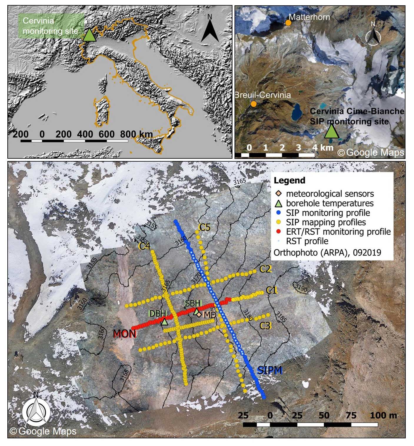
Figure 1The Cervinia Cime Bianche study site located in the Italian Alps, with the SIP monitoring profile (SIPM), ERT/RST monitoring profile (MON), borehole (shallow borehole (SBH) and deep borehole (DBH)), and meteorological sensor (MD) positions indicated. SIP data were collected along seven profiles, namely the SIP monitoring profile (SIPM), the SIP profiles C1–C5 collected for a spatial characterization of the site, and the long-term ERT/RST monitoring profile MON (red part of C1). The TINITALY digital elevation model (CC BY 4.0) was used as a base layer in the top-left panel. The satellite background image in the bottom panel is overlaid by an orthophoto of the survey area, including contour lines derived from the digital elevation model (ARPA).
In addition to the thermal and meteorological monitoring, annual ERT and RST (refraction seismic tomography) measurements have been collected since 2013 to observe long-term spatiotemporal permafrost dynamics at the site (Pogliotti et al., 2015; Pellet et al., 2016; Mollaret et al., 2019). Mollaret et al. (2019) observed a significant warming in the boreholes and electrical resistivity decrease from August 2013 and 2017 along the entire ERT/RST monitoring profile with estimated maximum ice contents of around 25 % (Mollaret et al., 2020).
2.2 Ground temperatures and meteorological data
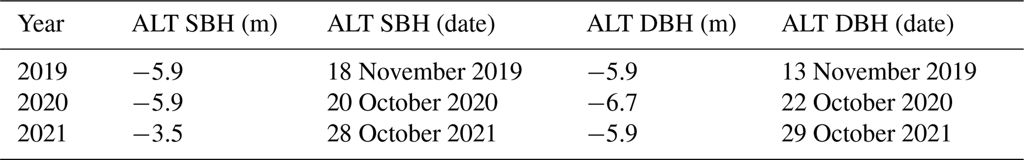
During the SIP monitoring period between September 2019 and September 2022, a mean annual air temperature (MAAT) of about −2.3 °C and a mean annual precipitation of about 1200 mm yr−1 were measured at the site. Strong winds contribute to the spatially changing snow cover thickness at the site, with less snow recorded at SBH compared to the DBH (Pogliotti et al., 2015), with a snow cover duration of ∼ 260 d yr−1 within the SIP monitoring period (i.e., Fig. 2a). The borehole temperature data indicate that the permafrost is at least 42 m thick (maximum depth of DBH; not shown in Fig. 2), with permafrost temperatures that vary between −0.3 and −1 °C (at 10 m depth; DBH), during the 3 years. Table 1 summarizes active layer thickness (ALT) evolution for the two boreholes with the highest values measured in October 2020 and lowest values reported in October 2021. The observed spatial variability in the ALT between the two boreholes (i.e., ∼ 2.5 m difference in ALT between SBH and DBH in 2021) can most likely be attributed to different ice water contents due to different surface and subsurface conditions in terms of the weathering and fracturing of the bedrock (Pogliotti et al., 2015).
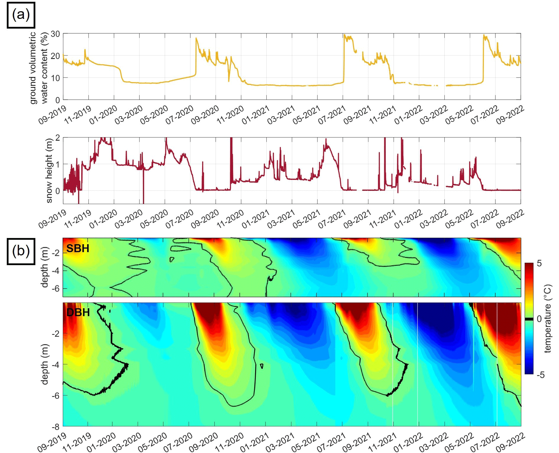
Figure 2(a) Ground volumetric water content measured at a depth of 20 cm and snow height measured at the position of the meteorological sensors and (b) borehole temperatures of the DBH and SBH for the SIP monitoring period between October 2019 and November 2022.
Seasonal variations in borehole temperature are consistent and correlate with air temperature, water content, and snow height. From Fig. 2, it is seen that the surface was covered by snow for about 260 d a year, with larger average snow heights in winter 2019/2020 (0.9 m) compared to 2020/2021 (260 d, 0.5 m) and 2021/2022 (190 d, 0.2 m). Due to the reduced insulating effect of relatively low snow height (e.g., Zhang, 2005), borehole temperatures reached the lowest values in winter 2021/2022. The highest air/surface temperatures were recorded in summer 2020 (not shown). And borehole temperatures were the highest in summer 2022 (due to earlier snowmelt). During the monitoring period under investigation, the behavior of the VWC is characterized by a steady minimum throughout the winter (6 %–7.5 %), followed by a strong increase at the beginning of the summer period (∼ 20 %) due to snowmelt (Fig. 2 and Pellet et al., 2016). The highest variability in the VWC can be observed during summer when precipitation is high.
Table 1Active layer thickness (ALT) evolution for the SIP monitoring period between October 2019 and August 2022.
2.3 Spectral induced polarization as monitoring method in frozen ground
2.3.1 The complex resistivity method
The induced polarization (IP) method, also referred to as the complex resistivity (CR) method, is a geophysical electrical technique which is based on measurements of the electrical impedance that can be performed in the time or frequency domain. When conducted in the frequency domain (as in our study), two electrodes are used to inject a sinusoidal current into the ground, and a second pair measures the resultant phase-shifted voltage. The impedance (Z∗) is then given as the amplitude ratio and phase shift between the measured voltage and the injected current. When performed at different frequencies (in the mHz–kHz range), commonly referred to as spectral IP (SIP), information on the frequency dependence of the electrical properties is gained. Multi-electrode measurements, in combination with inversion algorithms (e.g., Binley and Kemna, 2005), permit us to resolve for variations in the complex electrical resistivity (ρ∗) (or its inverse, the complex electrical conductivity (σ∗)) in the subsurface (e.g., Kemna et al., 2012). The complex resistivity can be written as its magnitude (|ρ(ω)|) (Ω m) and phase shift (ϕ) (rad) or expressed in terms of the real (ρ′(ω)) (Ω m) and imaginary (ρ′′(ω)) (Ω m) components, such as (e.g., Binley and Slater, 2020; Wait, 1984)
where ω represents the angular frequency (ω=2πf; f is the excitation frequency), and i is the imaginary unit (). The real and imaginary components of the complex resistivity account for energy loss associated with conduction and energy storage associated with polarization (capacitive property). In natural media, with a negligible number of electronic conductors, conduction takes place in the pore fluid through the migration of ions (electrolytic conduction; σel) and within the electrical double layer (EDL) present at the interface between grains and electrolyte (surface conduction; ) (e.g., Schwarz, 1962; Leroy et al., 2008). The EDL results from the attraction of counterions by charged mineral surfaces, depending on the surface charge and surface area. In the presence of an external electric field, charges in the EDL polarize resulting in the polarization effect (measured by the imaginary component of complex conductivity; ). Accordingly, for frequencies < 1 kHz, the complex conductivity σ∗ (or ρ∗)) can be written as (e.g., Binley and Slater, 2020)
In the measured frequency band, its frequency dependence can often be described by the Cole–Cole model (Cole and Cole, 1941).
Considering that field SIP devices are often limited in the frequency range and might lack the possibility for recovering the frequency maximum required to reliably fit a dispersion model such as the Cole–Cole, we propose here to quantify the frequency dependence in the SIP signatures using the phase frequency effect (ϕFE). Such a parameter represents the difference between the logarithms of the low-frequency and high-frequency ϕ values over a spread of frequencies (A) and normalized by the difference in the logarithms of the two frequencies, according to
where ω0 is the lowest frequency (in Hz), and the product Aω0 represents the maximum frequency investigated (in Hz). Grimm and Stillman (2015) proposed a similar analysis, but they only took into account the change in electrical resistivity over a spread of frequencies and ignored the polarization parameters (ϕ and σ′′).
2.3.2 Temperature dependence of electrical properties
The dependence of rock electrical properties on temperature differs for temperatures above and below the freezing point. Above the freezing temperature, in the presence of liquid pore water in a metal-free porous rock, the bulk electrical conductivity is controlled by the electrolytic conductivity of the liquid pore water and the surface conductivity, while the polarization effect for frequencies below 1 kHz is mainly related to electrochemical (ionic) polarization in the EDL at the pore water–solid matrix interface (Kemna et al., 2012). The temperature dependence of the electrical conductivity is controlled by the temperature dependence of the ionic mobility which is inversely related to the viscosity of the fluid and can be approximated by a linear relationship (Revil and Glover, 1998; Revil and Skold, 2011; Zisser et al., 2010). Within our analysis, we use a model by Oldenborger (2021) for the temperature correction of the bulk electrical resistivity, which can be written as
where αT and βT are temperature compensation factors for a fluid that depends on the choice of the reference temperature T0, and T is the temperature at which ρ is measured. Oldenborger (2021) derived different αT values of Eq. (6) (i.e., αT=0.02 °C−1, T0=20 °C; αT=0.0254 °C−1, T0=10 °C; αT=0.0321 °C−1, T0=0 °C).
Binley et al. (2010) measured the change in real and imaginary conductivity with positive temperature and reported an approximate increase in σ′ and σ′′ (at 1.5 Hz) with temperature of 2 % °C−1 using Eq. (6). Other empirical formulations modeled the temperature dependence of electrolytic conduction by an Arrhenius fit (e.g., Oldenborger, 2021).
When water changes its phase from liquid to solid, the salinity of the remaining liquid pore water phase increases (e.g., Hobbs, 1974; McKenzie et al., 2007). Above the eutectic temperature (i.e., the temperature at which water starts to crystallize) and below the freezing temperature, ionic exclusion leads to remaining salt within the pore water (e.g., Coperey et al., 2019; Oldenborger and LeBlanc, 2018; Revil et al., 2019) and an increase in fluid conductivity. During ice formation, the decrease in water content with temperature is gradual and follows a freezing curve (or thawing curve) (e.g., McKenzie et al., 2007). The saline unfrozen water is composed of residual water films (i.e., bound water) at the ice and mineral surfaces and water in smaller pores with a reduced melting point related to capillary and adsorptive forces according to the Gibbs–Thomson effect (see, e.g., Dash et al., 2006; Kemna et al., 2014a; Mohammed et al., 2018). Duvillard et al. (2018) and Coperey et al. (2019) extended the Stern layer model of Revil (2012, 2013b, a) to freezing conditions to describe the dependence of the electrical conductivity and the normalized chargeability on temperature below 0 °C, including parameters such as the residual water content, porosity, freezing, and characteristic temperature. Similar resistivity–temperature models were used to account for the temperature dependence of the electrical resistivity upon freezing for geophysical investigations in permafrost terrain (Oldenborger and LeBlanc 2018; Oldenborger, 2021).
2.3.3 Prediction of unfrozen water content and volumetric water content from petrophysical relationships
The distribution of subsurface electrical resistivity depends on soil properties such as saturation (Sw), fluid resistivity (ρw), or conductivity (σw) porosity (Φ) and surface conduction () (e.g., Lesmes and Frye, 2001), which can be written as
where m is defined as the cementation exponent, and n is the saturation exponent. While the saturation exponent varies in the range , the cementation exponent can range from 1 (for rocks with a low porosity but well-developed fracture network) to around 5 (for rocks with a low connectedness of the pore and fracture network) (Glover, 2009).
Neglecting the surface conduction, Oldenborger (2021) computes the volumetric water content (in percent) as a function of porosity and saturation (Sw), such as
with saturation being resolved from ERT data using the following relationship:
Within our study, we used the same value (i.e., 100 Ω m) for the pore water resistivity (ρw) as previous studies at the site (Mollaret et al., 2020) and estimated the cementation exponent for a given measurement of VWC with a constant factor a=1 and assuming n=2. In Eq. (9), ρcorr is the temperature-corrected bulk electrical resistivity at 0.5 Hz of Eq. (6). Upon freezing, Sw decreases and ρw increases due to ionic exclusion and estimates of the unfrozen water content S0, which is the fraction of water remaining unfrozen even at temperatures below 0 °C, can be derived by (Daniels et al., 1976)
with ρF being the resistivity of frozen and ρ0 of unfrozen material for which it is assumed that the pore space was completely saturated prior to freezing (S0=1). Using an exponential relationship for subfreezing temperatures,
Hauck (2002) and Oldenborger and LeBlanc (2018) derived estimates of the unfrozen water content as follows:
with the constant b being a function of depth.
2.3.4 Monitoring setup and acquisition of SIP imaging data
An array of 64 stainless steel electrodes with a separation of 3 m between electrodes connected with coaxial (shielded) cables, resulting in a profile length of 189 m, was permanently installed in October 2019 at the Cime Bianche plateau. The position of the SIP monitoring (SIPM) profile was chosen away from boreholes (see Fig. 1) and other metallic structures to avoid interferences due to high electrical conductivity. The position of the profile aimed at covering different surface characteristics, namely fine-grained and coarse-blocky areas and parts dominated by bedrock outcrops found along the study area towards the understanding of spatiotemporal SIP imaging results associated with different substrates during the SIP monitoring period.
Measurements were conducted with an eight-channel data acquisition system (DAS-1; manufactured by Multi-Phase Technologies). The configuration protocols consisted of dipole–dipole (DD) and multiple-gradient (MG) arrays and deployed coaxial cables to reduce cross-talking (e.g., Flores Orozco et al., 2013). During the SIP monitoring period, between October 2019 and August 2022, SIP data were collected at 12 different frequencies in the range between 0.1–225 Hz, using a DD configuration with dipole lengths of 12 m (skip-3) as normal and reciprocal (NandR) pairs for the quantification of data error (e.g., LaBrecque et al., 1996; Flores Orozco et al., 2012; Slater et al., 2000) and yielding a total number of 1474 quadrupoles (Table A1 in the Appendix). The MG configuration was deployed with a total number of 744 quadrupoles using four potential dipole lengths of 3, 6, 9, and 12 m within the current dipole in order to collect data sets with a higher signal-to-noise ratio (e.g., Dahlin and Zhou, 2006) compared to the DD configuration. The MG setup performed better during the winter period (between November and June), as poor galvanic contact between electrodes and the ground (also called contact resistance Rs) and low-current densities injected in frozen terrain covered by snow deteriorated the quality of the DD measurements. Mean current injections (I) varied between 0.2–15 mA throughout the whole SIP monitoring period and are listed for every measurement date in Table A1 in the Appendix.
Rs were recorded before each data acquisition with observed mean values between 20–160 kΩ. The highest Rs values were measured in the coarse-blocky part with observed values of 30–90 kΩ in the summer period and 125–190 kΩ in the winter months. Lowest values were observed for electrodes located in the fine-grained part of the profile with Rs values between 5–20 kΩ in summer and between 40–90 kΩ in winter.
During the SIP monitoring period, we avoided artificially wetting the electrodes for a reduction in Rs (e.g., Mollaret et al., 2019; Maierhofer et al., 2022) to ensure comparable conditions throughout the year (as proposed by e.g., Hilbich et al., 2011). We aimed at collecting an entire SIP data set once a month during a period of 2 years (between October 2019 and October 2021) to capture seasonal and annual changes in the polarization response. However, inaccessibility to the study area during the COVID-19 pandemic and technical problems led to gaps in the SIP monitoring data in December 2019 and December 2020, as well as the period between March and June 2020. In addition to the monthly measurements, we collected another end-of-summer data set in August 2022.
2.3.5 Data filtering, data error analysis, and inversion procedure of SIP monitoring data
We processed DD and MG data for every frequency and monitoring date independently, following the automated processing procedure presented in Fig. 3. For all DD data sets, we removed as erroneous readings those values that related to Rs>200 kΩ (considered an open circuit) and/or negative impedance magnitude (Z) values, as well as positive impedance phase values (ϕ). In case of DD measurements, outliers were identified (and removed) as those quadrupoles for which the misfit between normal and reciprocal impedance magnitude (ΔZ) and phase (Δϕ) readings was larger than 50 % of the average value (ZNR, ϕNR) and larger than twice the standard deviation of the NandR misfit of the entire data set, similar to Maierhofer et al. (2022). For MG surveys, where no reciprocals were measured, we developed an analysis scheme for data quality that considers the relationship between phase and voltage readings to assess signal strength and a moving average filter to remove spatial outliers and erroneous measurements (see Fig. 3). In other words, we removed isolated readings based on plots from phase readings plotted against their associated voltages. The resulting numbers of data after filtering are summarized in Table A1 (Appendix) for each survey.
After the analysis of the independent data sets, we analyzed the temporal evolution of the number of quadrupoles for each frequency. This is needed to ensure that imaging results obtained from different times are related to a similar resolution. Due to the high number of outliers detected for winter measurements (up to 80 % for 75 Hz), we did not systematically remove unrepeated quadrupoles for the entire SIP monitoring period. We performed the analysis for detailed processes: (1) the thawing of the active layer during the summer period (June to October 2020) and (2) the inter-annual changes based on summer measurements (August 2020, 2021, and 2022). For those two specific analyses, only repeated quadrupoles were used for inversion.
For the quantification of data error in the inversion, we used a linear model describing the uncertainty in impedance magnitude (s(ZNR)) as a function of ZNR (i.e., LaBrecque et al., 1996)
with parameters a and b denoted as the absolute (Ω) and the relative (%) error
For the quantification of data error in the impedance phase readings, we applied a constant error model (i.e., no dependence on the impedance magnitude or phase values), obtained as sd(ϕNR) (mrad), similar to the approach by Slater and Binley (2006).
The NandR analysis revealed a significant increase of 30 %–50 % in the error parameters (i.e., a and b) for the winter measurements, demonstrating lower signal-to-noise (S/N) ratios in winter which are expected to result in higher uncertainties in the imaging results obtained for measurements between January and May. Different SIP monitoring studies (e.g., Lesparre et al., 2017; Flores Orozco et al., 2019) use the same error parameters for the inversion of the entire monitoring period, assuming that this permits the comparison of imaging results obtained with the same level of contrasts, i.e., sensitivity. However, such an approach assumes a fairly consistent S/N across the monitoring data set. Accordingly, within our analysis, assuming the same error parameters for the entire SIP monitoring period leads to either under-fitting the readings in summer (assuming the error level from winter measurements) or over-fitting the winter data when inverted to the error parameters observed in summer measurements. Hence, we define error parameters for each data set collected at different times and frequencies, which also considers the frequency dependence observed in our data with higher misfits detected for higher frequencies compared to lower frequencies (similar to Flores Orozco et al., 2011). Additionally, we used the same error parameters for DD and MG data, since error models allow the use of the same error parameters for configurations where no reciprocals are available.
For the inversion of the SIP data, we used the finite-element smoothness–constraint inversion code CRTomo (complex resistivity tomography; Kemna, 2000) which computes the distribution of the complex resistivity in the subsurface from a given data set of impedance magnitude and phase values at a distinct frequency. Data error estimates are defined in the inversion and permit fitting the observed data within its noise level, which is defined by an error model (Kemna, 2000). The iteration is stopped if the root mean square (rms) difference between model response and data, which includes a normalization of the individual misfits by the error taken from the error model, reaches a value below its target value of 1, after which smoothing is again increased until the rms value is equal to 1 (within a tolerance interval). The inversions converge to the target value fitting the observed data within their estimated noise level for the smoothest possible model.
To assess the reliability of the monitoring inversion results, especially regarding the resolved electrical properties at depth, we make use of the depth of investigation (DOI) index, introduced by Oldenburg and Li (1999), which is based on two 2D inversions of the data set using different values of the reference complex resistivity model. In our analysis, we calculated the DOI value for a model cell given by
where m1r=1000 Ω m, −5 mrad is the first reference model, m2r=10 000 Ω m, −75 mrad is the second reference model, and m1(x,z) and m2(x,z) are the model cell resistivity and phase values from the first and second inversion. DOI values are computed for resistivity and phase images and applied separately to the corresponding images. We chose the values of the reference models as mean minimum and maximum resistivity and phase values observed in all SIP images. We blank model regions with large DOI values (i.e., > 0.2, as proposed by Oldenburg and Li, 1999) in all imaging results for all frequencies presented in this study.
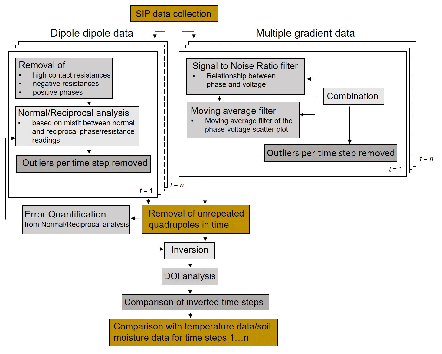
Figure 3Workflow of SIP data processing for the monitoring data set at Cime Bianche, Cervinia.
2.4 Complementary geophysical data sets
In September 2019, we collected ERT data along five profiles, C1, C2, C3, C4, and C5 (Fig. 1), using the DAS-1 device with a DD configuration with dipole lengths of 12 m (skip-3). For profiles C2, C3, and C5, 32 electrodes and a separation of 4 m were chosen, whereas profiles C1 (prolongation of the ERT/RST monitoring profile) and C4 consist of 64 electrodes and a 2 m separation. Data quality was evaluated by means of NandR analysis, and the inversion of the resistivity data at 0.5 Hz was performed in 3D using the modules of the open-source library pyGIMLi (Rücker et al., 2017). We used mean error parameters (α=0.1 Ω, b=5 %) from NandR analysis for the inversion of the ERT data sets to fit all data to the same error level enabling a better comparison of the multi-dimensional (different profiles and frequencies) inversion results, similar to Lesparre et al. (2017).
Refraction seismic tomography (RST) measurements were conducted along the SIP monitoring profile in August 2020 with a 24-channel Geode instrument (manufactured by Geometrics) and 24 geophones (corner frequency of 30 Hz) with a roll-along of a 12-geophone overlap. In total, 36 receiver and 14 shot locations were used, with ∼ 15 individual shots recorded between electrode 12 and 48 (between profile meter 33 and 141), keeping the same geophone spacing as for electrodes. We used a sledgehammer as a source of the seismic waves with hit points between every second geophone along the seismic refraction line. The individual shots were stacked ∼ 10 times to improve the signal-to-noise ratio of the seismic data. First-break travel time picking was manually done, using the open-source library formikoj (Steiner and Flores Orozco, 2023), which provides modeling, reading, and basic processing of seismic waveform data. A 120 Hz low-pass filter was applied to the seismic traces to mitigate the influence of high-frequency noise. For the independent inversion of the picked P-wave travel times, we used the modules of the open-source library pyGIMLi with an estimated RST data error of 2.2 ms from comparing a subset of travel times that was picked twice.
We used the PJI framework developed by Wagner et al. (2019) to quantify the four volumetric fractions of ice (fi), water (fw), air (fa), and rock matrix (fr), based on the filtered apparent resistivity values and picked P-wave travel times. We used the same porosity and seismic velocity values as in Mollaret et al. (2020), i.e., an initial porosity of 40 % and constituent velocities (vp) of 1500 m s−1 for pore water, 3750 m s−1 for ice, 4000 m s−1 for the rock matrix, and 330 m s−1 for air. We accounted for surface conductivity in addition to electrolytic conduction by introducing a constant surface conductivity term in Archie's law. We tested inversions with a surface conductivity range between 0.001 and 0.01 S m−1 (based on laboratory studies on pure ice (Bullemer and Riehl, 1966; Caranti and Illingworth, 1982) and rock samples under freezing conditions (Coperey et al., 2019)) and chose a final constant value across the imaging plane of 0.01 S m−1 as it resulted in the lowest chi-square (χ2). A relative error of 5 % was used for the ERT data following the NandR analysis and an absolute error of 2.2 ms for the picked travel times in the inversion, which resulted in an error-weighted χ2 fit of 1.0. The final PJI results are presented in Appendix C.
2.5 Complementary SIP laboratory data
Laboratory measurements were performed on a cylindrical solid-rock sample of 10 cm length and 3 cm diameter of amphibolite (with a porosity of 3.5 %) and a loose-sediment surface sample, both collected close to the SIP monitoring profile. The electrical impedance was measured in a frequency range of 10 mHz to 45 kHz during controlled freeze–thaw cycles (+20 to −40 to +20 °C) using a four-channel SIP-04 impedance spectrometer (Zimmermann et al., 2008) and is shown in the Appendix B. The solid-rock sample was fully saturated with water of similar fluid conductivity to that in field conditions (0.01 S m−1). For this purpose, diluted tap water was used to obtain an electrolyte with a distribution of ions that resembles realistic field conditions. Afterwards, the sample was sealed in a shrinking tube and placed in a climate chamber where it was cooled down from +20 to −40 °C by successively changing the temperature in steps of 0.2–4 °C with a duration of 120 to 180 min for each temperature step. Limbrock et al. (2021) found such settings to be sufficient for the given size and thermal properties of the sample to reach thermal equilibrium. After one freezing cycle, the samples were heated up again, following the same temperature procedure. For potential measurements, we used ring electrodes made out of tinned copper with a distance of 3 cm and plate electrodes made out of stainless steel for current injection. The loose-sediment sample was saturated up to a volumetric water content of about 20 %, with the same type of water and placed in a cylindrical container with a total length of 18 cm, a diameter of 4 cm, and a potential electrode separation of 6 cm. Potential electrodes were made out of copper and current electrodes out of bronze. Due to the increased sample size, the duration of each temperature step was increased by 60 min. During freezing, we had to ensure a direct contact of the potential electrodes and the measured sample. Investigations concerning possible sources of error arising due to the contact between potential electrodes and the tested sample were out of scope of this study and are further discussed in, e.g., Wang and Slater (2019).
3.1 Site characterization
In Fig. 4, we present 3D electrical resistivity results as slices extracted at different depths parallel to the surface obtained from the 3D inversion of the five ERT profiles (C1–C5) collected in September 2019. Figure 4 shows lower electrical resistivity values in the shallow subsurface (0–4 m depth) than for deeper layers (> 5 m depth), with slightly lower values observed in the western compared to the eastern part of the study area. The thickness of the low-resistive surface layer (inflection point in electrical resistivity) is slightly overestimated compared to the thaw depth measured in the boreholes at the date of the geophysical measurements (Fig. 4g), most likely due to the smoothing in the inversion. Low electrical resistivity values (< 8000 Ω m) are observed in the northern and the central–western part of the study area for all depths, whereas the highest electrical resistivity values (∼ 30 000 Ω m) are observed at > 5 m depth in the central, central–eastern, and central–southern parts of the study area. Between 6 and 20 m depth, we observe no strong resistivity changes associated with the permafrost body.
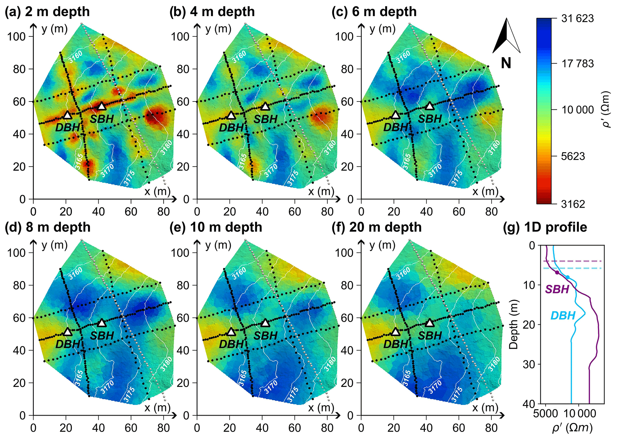
Figure 4Spatial characterization of the Cime Bianche monitoring site based on the 3D electrical resistivity inversion results from five profiles collected in September 2020 (dotted black lines). Panels (a)–(f) represent slices parallel to the surface at six different depths. The borehole location of the SBH and the DBH are marked, and white contour lines represent the surface elevation. The coordinates of the SIP monitoring profile are shown in addition (dotted grey line), but these data were not used for inversion due to a differing measurement date (October 2020). Panel (g) represents the resistivity–depth profiles at the location of the two boreholes with the measured thaw depth (dashed lines) and the inflection point in the resistivity data (dots).
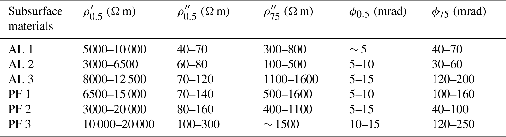
The baseline SIP imaging results along the permanent SIP monitoring profile of October 2019 are presented in Fig. 5 and expressed in terms of the phase (ϕ), the real (ρ′), and the imaginary (ρ′′) components of the CR, as obtained for data collected along the SIP monitoring profile for low (0.5 Hz) and high (75 Hz) frequencies. While the frequency dependence is pronounced in the polarization parameters (for ρ′′ and ϕ), we observe no significant variation in ρ′ with increasing frequency for the whole imaging plane. Similar to the results shown in Maierhofer et al. (2022), absolute ρ′′ and ϕ values are higher for 75 Hz (hereafter and ϕ75) than for 0.5 Hz ( and ϕ0.5). Comparatively low values are resolved at depths < 4 m for , , and ϕ75 and < 5 m for ϕ0.5, which can be related to the 4 m thick thaw layer composed of fine- to coarse-grained material (see the surface characteristics shown in Fig. 5a). The thaw layer is underlaid by a high-resistivity layer with high absolute ϕ0.5 and ϕ75 values, which is representative of the permafrost body (e.g., Table 2). The contrast between the two layers is highest for and ϕ75.
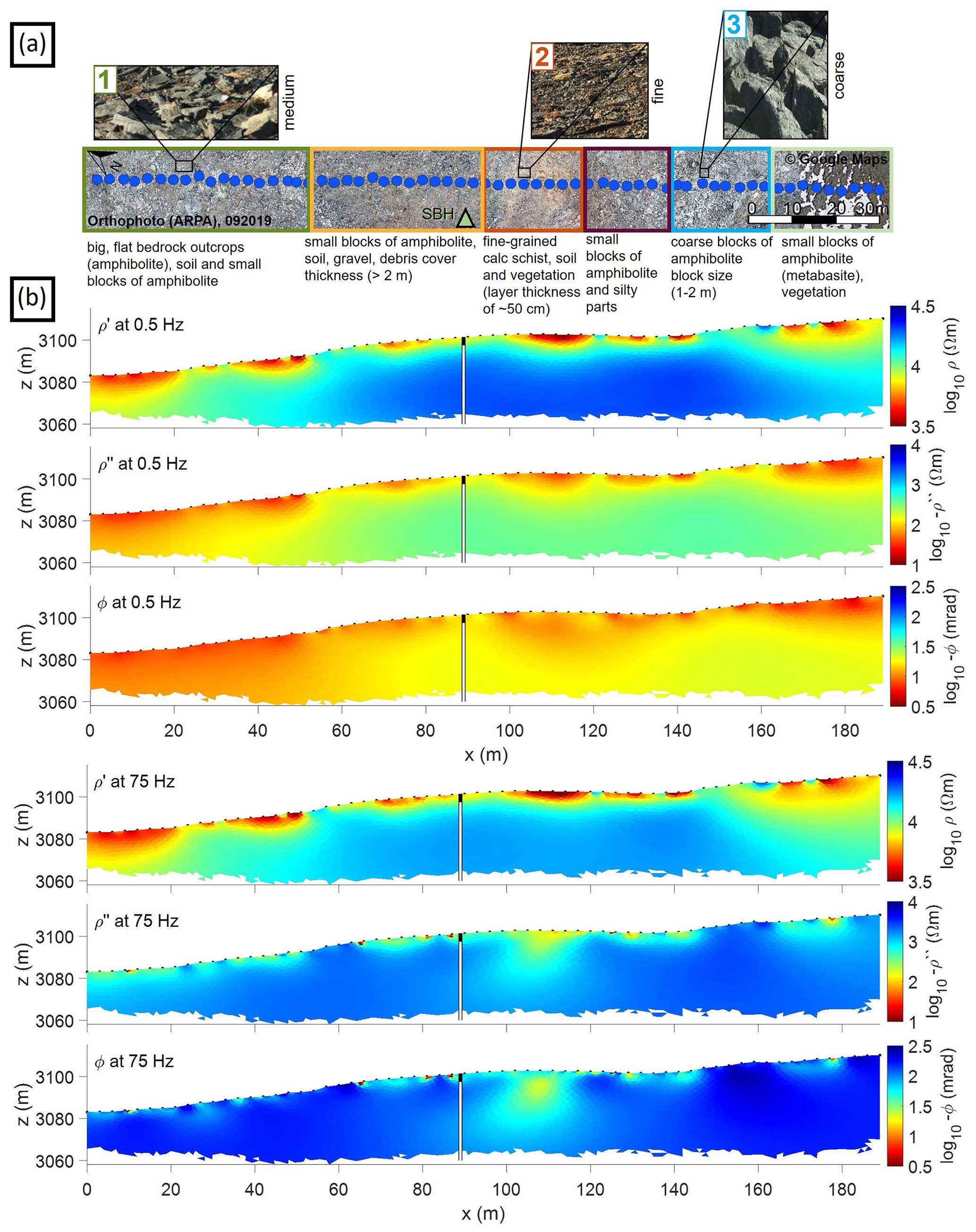
Figure 5SIP baseline imaging results, corresponding to data collected in October 2019. Panel (a) represents different substrate classes, which are discussed in more detail in Sect. 4. (b) Baseline complex resistivity model (October 2019) are shown at two frequencies (0.5 and 75 Hz) with the two boreholes located at the center of the profile (the SBH 20 m away; the DBH 50 m away), and the black layer represents the thaw depth at the measurement date. The satellite background image in panel (a) is overlaid by an orthophoto of the survey area derived from the digital elevation model (ARPA).
Concerning lateral changes in the SIP images, the highest electrical resistivity and absolute ϕ75 are observed for all depths between profile meter 138 and 162 (e.g., within the permafrost (PF) 3 in Table 2), corresponding to the coarsest amphibolite blocks of 1–2 m size found at the surface of the SIP monitoring profile (see Fig. 5a). The uppermost 1–3 m of profile meter 93 to 117 reveal the lowest resistivity values and absolute phase values at 75 Hz (e.g., PF 2 in Table 2) along the profile, which can be related to a thin layer of silty soil with some vegetation and fine-grained calc-schists observed at the surface (see Fig. 5a). The contrast to the frozen bedrock (∼ 1.2 m) is clearly visible for this part of the profile for all components of the complex resistivity, except for and ϕ75, where we resolve a low-polarizable anomaly also at depth ( Ω m, ϕ75<60 mrad). In the northern part of the monitoring profile with intermediate grain size (between 0 and 51 m), we observe low real resistivities and absolute phase values at the surface (e.g., within the active layer (AL) 1 in Table 2) and at depth (e.g., PF 1 in Table 2) for 0.5 Hz and intermediate absolute phase values for 75 Hz (see Table 2).
Table 2Range of complex resistivity values observed along the SIP monitoring profile within the active layer (AL) and the permafrost body (PF).
3.2 The temperature dependence of the SIP method
Figure 5 reveals clear variations in the polarization for different depths (i.e., temperatures) and frequencies. To better understand the temperature dependence of the polarization response, we show in Fig. 6a the measured impedance field data (apparent resistivity magnitude ρapp and phase ϕapp) in the active layer in a frequency range of 1–75 Hz between October 2019 and November 2021, including the warm (i.e., summer months from July to October) and cold (i.e., winter months from November to May) periods. For comparison, Fig. 6b shows SIP laboratory data in the same frequency range measured over a thawing cycle from −10 to +10 °C.
For both laboratory and field data, we observe a clear distinction in the polarization response between unfrozen and frozen states. Absolute phase values are low for positive temperatures (summer months) and show no significant frequency dependence, whereas if temperature decreases (during winter), we observe an increase in absolute ϕapp values 8 times higher than in unfrozen state between 1 and 75 Hz. This increase in the absolute phase for subfreezing temperatures starts at a frequency of 7.5 Hz for the field data, at ∼ 10 Hz for the loose-sediment sample, and at ∼ 50 Hz for the solid-rock sample. Thus, the inflection point seems to change depending on the texture/ice content. Such an effect can be related to the well-known temperature-dependent relaxation behavior of ice, with its maximum in the kilohertz range (as shown for the full spectrum between 10 mHz and 45 kHz in Appendix B). Additionally, the increase in absolute ϕapp values with increasing frequency is more pronounced for the loose-sediment sample (45 mrad at −10 °C) than for the solid-rock sample (15 mrad at −10 °C), suggesting an enhanced response with increasing ice contents. Accordingly, the frequency dependence in the phase measurements might be used as a proxy to discriminate between regions with no ice and regions richer in ice, as also observed in Maierhofer et al. (2022). Clearly, the frequency range in the SIP data needs to extend above this sensitive frequency, which corresponds to an inflection point between the low response (likely due to the geology) and the high values associated with ice. When comparing the SIP monitoring and laboratory data, we find a similar behavior in the polarization during freezing and thawing cycles; however, the increase in absolute phase is smaller for laboratory data (2–15/5–45 mrad for the rock/sediment sample) than for field data (35–290 mrad) in the temperature range covered by both data sets (−8 to +10 °C observed within the active layer at our field site).
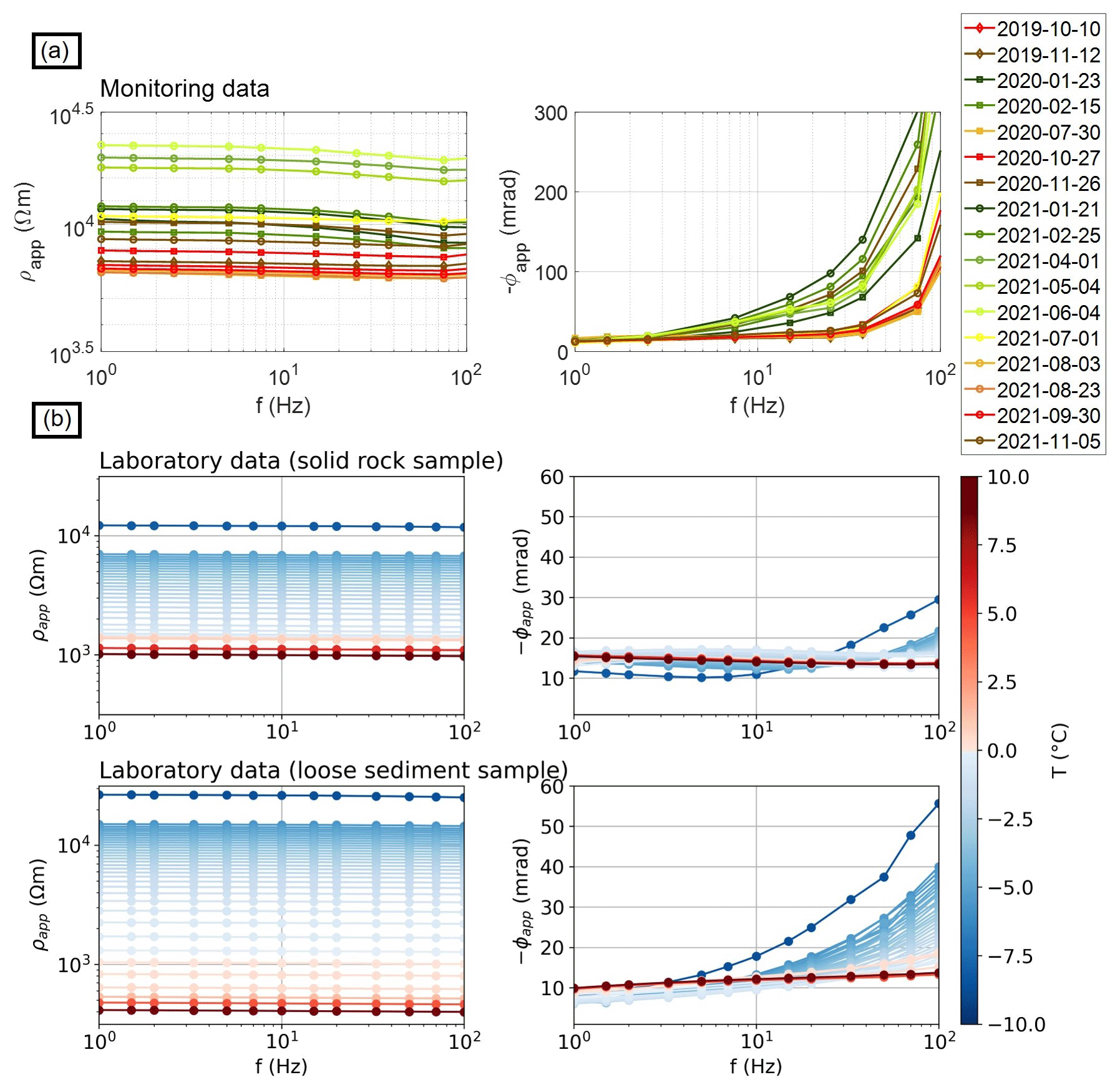
Figure 6(a) Temporal changes in SIP measurements between October 2019 and November 2021 (frequency range 0.5–75 Hz). Impedance magnitude is expressed in terms of its phase and magnitude (converted to apparent resistivity) values and shown for level 1 and 2 (i.e., 3 and 6 m electrode separation between current and potential dipoles, which corresponds to the active layer) at a horizontal distance of 80 m. Different symbols and colors represent different years and months, respectively. Variations in ρapp and ϕapp between summer and winter are linked to seasonal temperature variations between +10 and −8 °C measured in the borehole close to the subsurface. (b) SIP laboratory measurements on a solid-rock sample and a loose-sediment sample collected at the site close to the monitoring profile for a frequency range between 1 and 75 Hz and temperatures between −10 and +10 °C.
3.3 The phase frequency effect and its link to temperature, water content, and ice content estimates
Figure 6a shows that our SIP field data do not capture the peak in the frequency dependence, which, according to, e.g., Auty and Cole (1952), would be expected between 4 and 11 kHz for pure ice but extend above the inflection point associated with a sensitive frequency, where phase values increase with increasing frequency and ice content. Hence, we propose to analyze the phase frequency effect (ϕFE) presented in Eq. (5). To evaluate the applicability of such parameter, we present in Fig. 7 the lab measurements collected during freezing and thawing cycles in terms of Eq. (7a) apparent resistivity (ρapp at 0.5 Hz) and for the Eq. (7b) ϕFE (calculated between 70 and 0.5 Hz).
After saturating and during cooling both samples from +10 to ∼ 0 °C, both ρapp and ϕFE follow a linear trend, with values increasing with decreasing temperature. During initial freezing, supercooled conditions (i.e., water remaining liquid below its freezing point) with constant ρapp and ϕFE values occur between 0 and −2.8 °C for the loose-sediment sample and between 0 and −2.8 °C for the solid-rock sample. An exponential increase in ρapp (3 kΩ m °C−1 for the sediment sample; 1.9 kΩ m °C−1 for the rock sample) and ϕFE (0.044 °C−1 for the sediment sample; 0.031 °C−1 for the rock sample) is observed below this temperature, which is indicative of abrupt ice formation in the pores of the samples. During thawing from −10 to −0.1 °C (for the loose-sediment sample), respectively, −0.7 °C (for the solid-rock sample), ρapp and ϕFE gradually decrease with a smaller average rate of change for the rock sample (1.4 kΩ m °C−1, 0.021 °C−1) than for the sediment sample (3 kΩ m °C−1, 0.03 °C−1), suggesting continuous melting of ice in the pore space.
During thawing, ρapp and ϕFE are generally higher than during freezing (ΔϕFE=0.05). Upon freezing, supercooling leads to a remaining unfrozen pore fluid below the freezing point until ice starts to form, thus resulting in a larger amount of unfrozen water compared to thawing processes at the same temperature (Wu et al., 2017). Additionally, we observe a lowering of the freezing point of water (from 0 to −2.5 °C), which can be explained by an exclusion of ions from ice formation and accumulation in the liquid phase (as further discussed by Bittelli et al., 2004). At subfreezing temperatures, ρapp and ϕFE values are generally higher for the loose-sediment sample, which can be explained by a higher ice content of the loose-sediment sample compared to the solid-rock sample. Hence, from Fig. 7, we depict a clear dependence of the ϕFE on temperature and ice content.
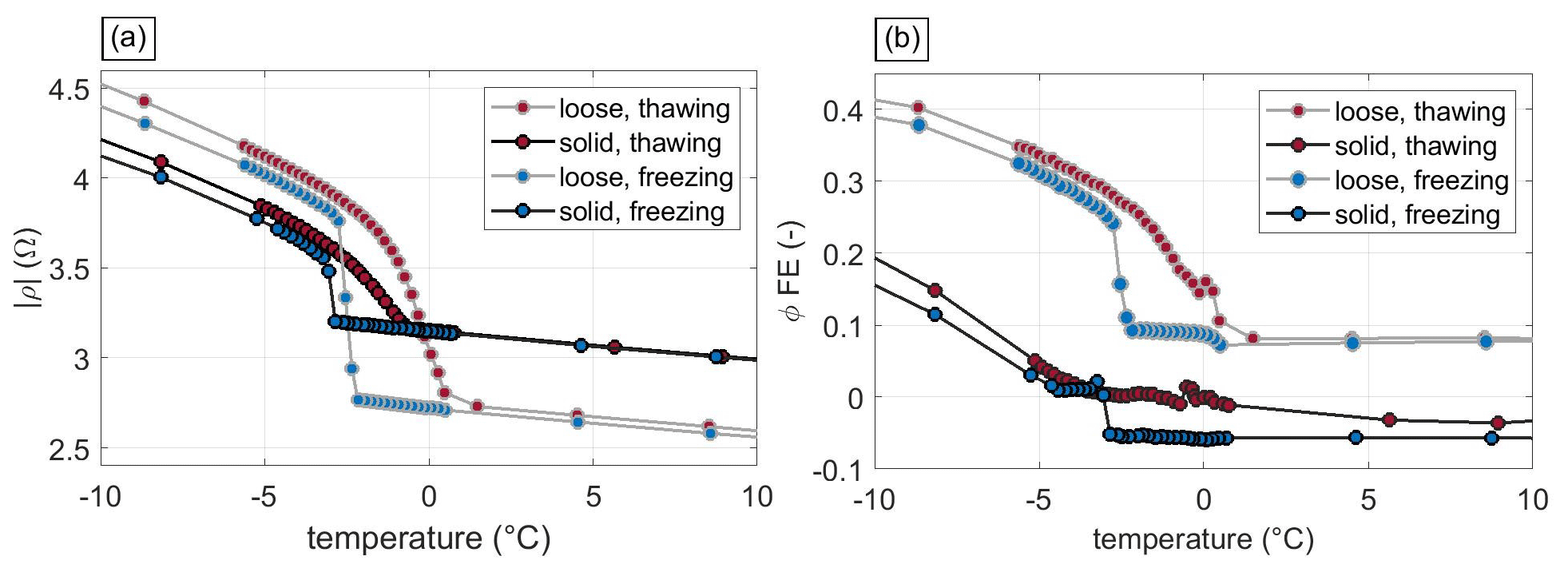
Figure 7Temperature dependence of (a) the impedance magnitude (at 0.5 Hz) and (b) for the ϕFE (calculated between 70 and 0.5 Hz) measured on solid-rock (solid) and loose-sediment (loose) samples during freezing (blue) and thawing (red) in the laboratory (same experiments as shown in Fig. 6).
Figure 8 shows the spatial variation in the ϕFE computed from the inversion of field data collected in August 2020 along the SIP monitoring profile. To investigate a possible correlation with ice and water content, we compare this image with PJI-estimated volumetric ice and water contents (fi, fw) based on ERT and RST data collected on the same day in the same profile. The complete PJI results (electrical resistivity, seismic velocities, and rock and air contents) are presented in Appendix B.
The ϕFE in Fig. 8c ranges from 0.2 to 0.4, similar to the values observed in the laboratory, and is highest at 5–10 m depth (∼ 0.35 at the borehole location) and lowest in the thaw layer (< 0.3 at the borehole location). Figure 8a–b reveal that PJI-estimated fi values are minimal (∼ 7 %–10 %), and fw reaches its maximum (10 %–33 %) in the thaw layer. Highest fi (∼ 22 % at the borehole location) and lowest fw (∼ 4 % at the borehole location) are encountered between 5 and 10 m depth. The comparison of vertical 1D logs of ϕFE, fi (Fig. 8d) and fw (Fig. 8e) extracted at the borehole location from the 2D sections suggests a high and positive linear correlation between ϕFE and fi (r2=0.9) and a lower and negative correlation between ϕFE and fw (r2=0.5). In general, there is a good correlation between low ϕFE and low fi and high fw, while high-ϕFE values correspond also with high fi and low fw, supporting our hypothesis that the phase frequency effect can be used as a proxy for the ice content – and indirectly temperature and water content. The main inconsistency between the three parameters can be observed between 90 and 115 m, where a low-ϕFE anomaly coincides with high fi. Within this part of the profile, we observe at the surface the material with the finest texture (i.e., silty soil; box 2 in Fig. 5a) with calc-schists visible at the surface. Hence, the polarization parameter might be able to resolve a decrease in ice content that the PJI is not able to resolve due to the lack of sensitivity of electrical resistivity and seismic velocities to textural properties.
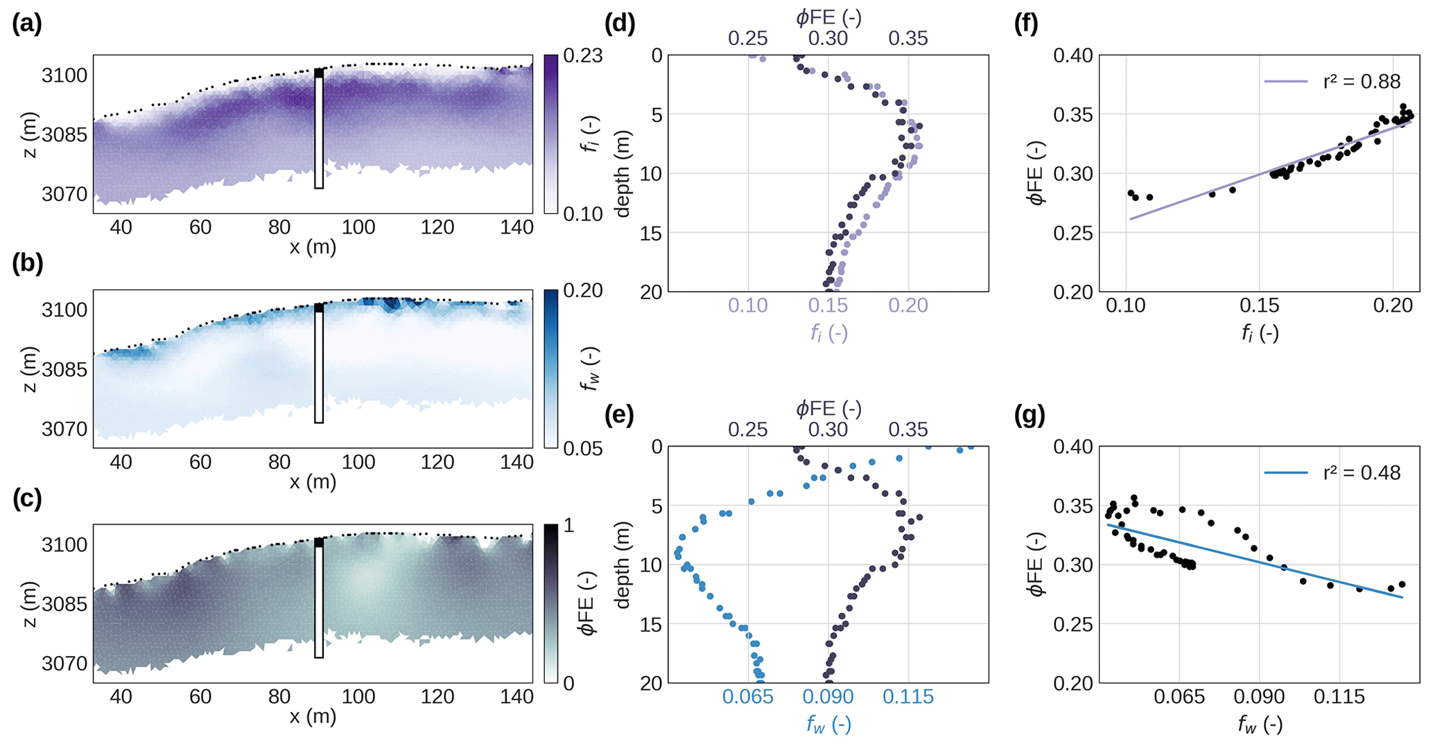
Figure 8(a–c) Calculated ϕFE for the phase of the complex resistivity imaging results between 75 and 0.5 Hz and visualized for the whole tomogram for the SIP monitoring profile (between profile meter 33 and 141) and comparison with water and ice content estimates from PJI results. (d) Vertical 1D logs of the ϕFE and the ice content and (e) water content extracted at the borehole location from 2D sections.
3.4 Temporal changes in the SIP results
In Fig. 9, we show the temporal evolution in borehole temperatures and the complex resistivity at different frequencies (0.5, 7.5, 25, and 75 Hz) extracted for the borehole location at different depths. During the 2-year monitoring period, we observe that complex resistivity results mainly follow the thermal evolution but with distinct differences between the 2 years. Freezing started in both years (2019 and 2020) in November, with the advance of the freezing front reflected in a decrease in temperature and an accelerated increase in the electrical parameters. The winter of 2020/2021 was much colder than that of 2019/2020, which is represented by ∼ 2 times higher ρ′, similar ϕ0.5 and more than 3 times higher Δϕ75 values in January 2021 compared to January 2020. Borehole temperatures, ρ′, and ϕ reached their minimum and maximum values, respectively, between January and March 2021 ( °C, kΩ m, ϕ0.5=60 mrad, ϕ7.5=180 mrad, ϕ25=450 mrad, and ϕ75=2000 mrad). During spring 2021 (April–June), a steady increase in shallow-borehole temperatures lead to seasonal ice melt in the uppermost layer and a small decrease in shallow electrical parameters. An abrupt increase in subsurface temperatures at the end of June 2021 is reflected in a decrease of 30 % in ρ′, a decrease of 85 % in ϕ0.5, and a decrease of 90 % in ϕ75. Between March and June 2020, no SIP measurements were conducted. During summer 2021, we observe smaller shallow absolute ϕ values compared to the summer period in 2020, which can be explained by a higher VWC observed in summer 2021 than in summer 2020 (i.e., Fig. 2).
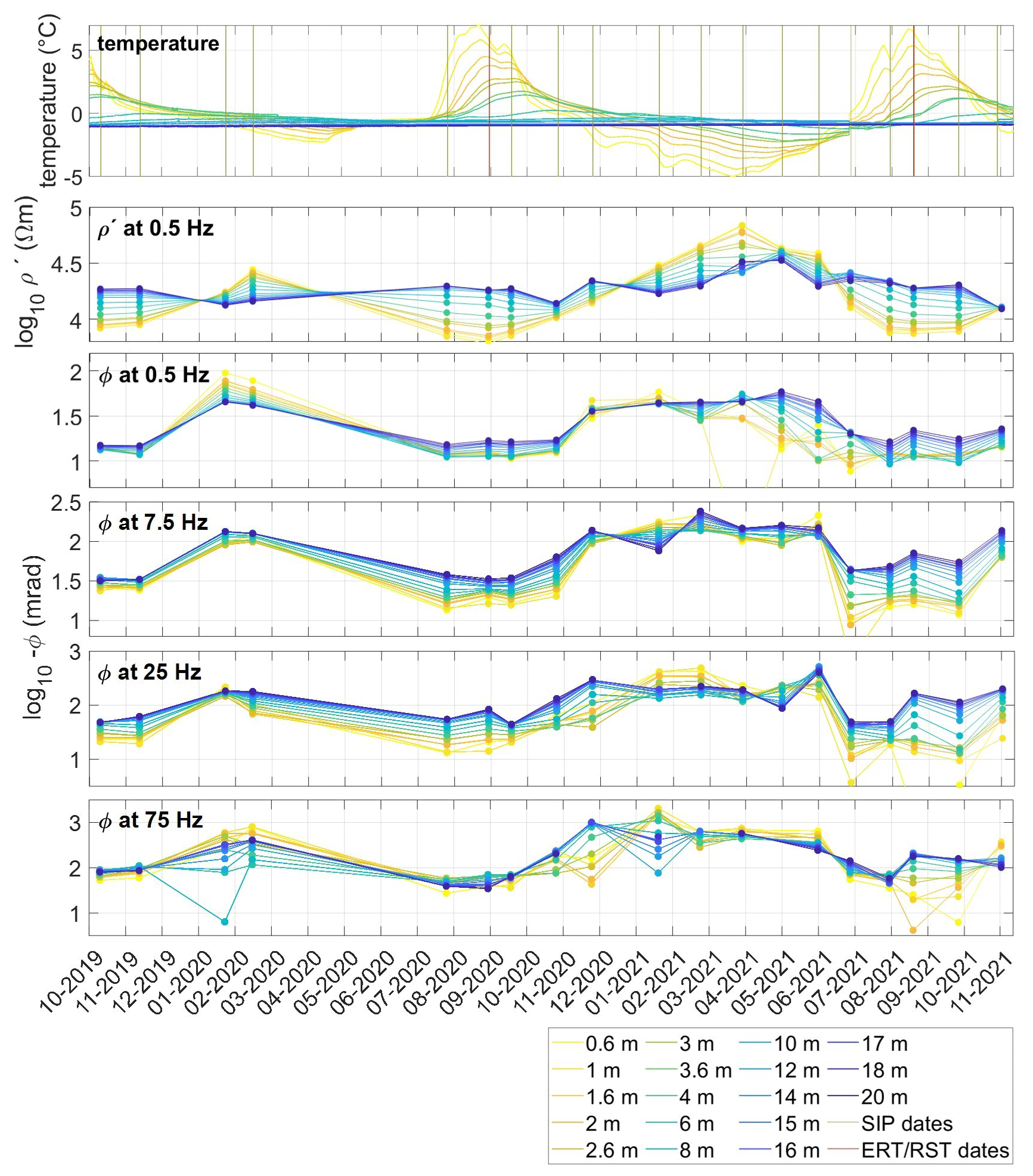
Figure 9Comparison of borehole temperatures with complex resistivity results at different frequencies (0.5, 7.5, 25, and 75 Hz) extracted at the borehole position in the borehole temperature sensor depths.
3.5 Complex resistivity–temperature relationship
Figure 10 presents the complex resistivity (ρ∗) data extracted from the SIPM inversion results at the borehole location for four frequencies and a comparison to the borehole temperatures (T). The T-ρ∗ relationship is shown for two material compositions: debris (Fig. 10a) and bedrock (Fig. 10b), with the transition between debris and bedrock at the borehole location estimated at a depth of 1.2 m (for further details, see Appendix B). The T-ρ∗ relationship was fitted for each frequency using a linear model for positive temperatures and an exponential model for subzero temperatures with the coefficients of determination obtained for the two regions and different frequencies summarized in Table D1 of Appendix D.
For unfrozen conditions, we observe that ρ′ and absolute ϕ values are similar for debris and bedrock and show a linear increase in both parameters with decreasing but still positive temperature. The increase is higher for ρ′ compared to ϕ. Additionally, ρ′ and ϕ values are higher at 75 Hz than at 0.5 Hz (with a difference between them of 700 Ω m and 50 mrad).
Below the freezing point and for both material compositions, ρ′ and absolute ϕ increase exponentially with decreasing temperatures, with the highest absolute ϕ and lower ρ′ values observed at 75 Hz compared to 0.5 Hz. The frequency effect in ϕ at −1 °C is different for debris and bedrock, with a pronounced increase in ϕ for the debris (310 mrad) resolved for data at 0.5 and 75 Hz. Such high ϕFE reflects the expected high ice contents in winter periods in the small to coarse blocks found at the surface. Accordingly, we observe a modest change in the phase values (70 mrad) for the bedrock, where we have lower porosity and, thus, also lower ice contents. These results correspond to the laboratory results in Fig. 7, indicating that ϕFE is higher for loose sediment at subfreezing temperatures.
In the freeze–thaw transition processes, hysteresis effects are often also observed at the field scale, as shown by Mollaret et al. (2019) and Wu et al. (2013). In Fig. 10c, we present the seasonal cycle at shallow depths (within the debris layer), where freezing and thawing processes can be distinguished in ρ′ and ϕ at 7.5 Hz (which represents the sensitive frequency) and for the ϕFE calculated between 0.5 and 75 Hz. Similar to the laboratory results, we also observe at the field scale lower ρ′ and ϕ values and slightly lower ϕFE during freezing (from October to January) than during thawing (from May to July), which is related to the difference in liquid water content for the two processes. While ρ′, ϕ, and ϕFE values are small in October/November, an increase occurred in January–February, with peak values detected between February and May. During snowmelt in May–June, the ρ′, ϕ, and ϕFE values drop abruptly, with the absolute phase at 7.5 Hz decreasing from 100 to 10 mrad and the ϕFE falling below 0.25 as soon as water content increases. The zero-curtain effect could not be observed during the phase change as the temporal resolution of the monitoring was too low during this period.
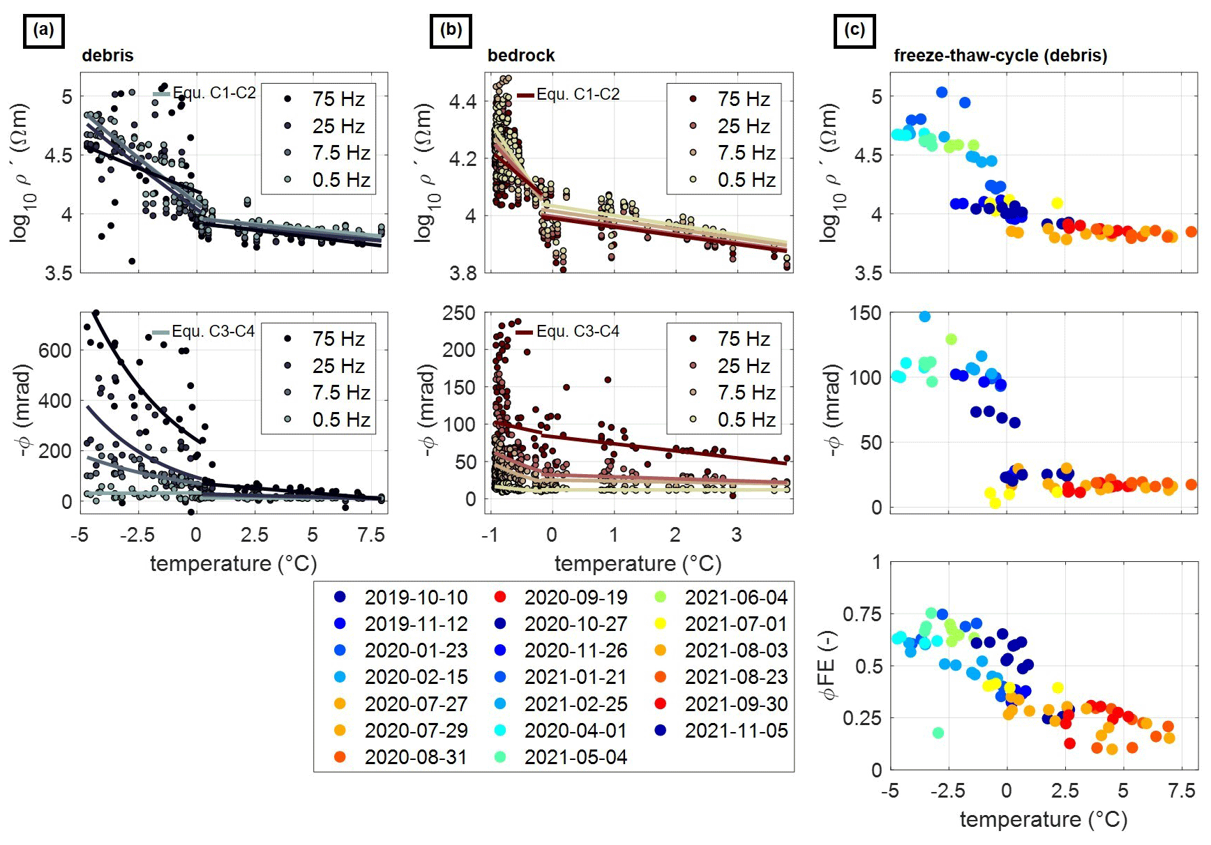
Figure 10Temperature dependence of the complex resistivity at different frequencies (0.5, 7.5, 25, and 75 Hz) obtained from 2-year SIP monitoring data extracted at borehole location for all temperature sensor depths down to 20 m. (a) Debris (< 1.2 m depth). (b) Bedrock (> 1.2 m depth). The data were fitted for each frequency using a linear model for positive temperatures and an exponential model for subzero temperatures, according to Eqs. (D1)–(D4) in Appendix D. In panel (c), we show the temperature–resistivity relation, temperature–phase relation at 7.5 Hz, and the temperature–phase frequency effect relation for the debris for all available dates.
4.1 Reliability of SIP monitoring measurements
We investigated the subsurface polarization properties for both seasonal and inter-annual changes along a transect located in a mountain permafrost environment in the Italian Alps. Our monitoring results reveal an overall increase in resistivity and phase of the complex resistivity during the winter months. However, such an increase is also observed at larger depths (i.e., > 10 m) where expected changes in temperature, water content, and ice content are small. High phase readings in winter are partly due to low current densities injected in frozen terrain covered by snow, resulting in low S/N ratios, and partly also due to parasitic electromagnetic fields in the measurements. While inductive coupling effects can be neglected in our case, as the high resistivity of the substrate shifts inductive coupling to higher frequencies mainly affecting data in the kHz range, parasitic capacitive coupling (PCC) needs to be considered due to current leakage associated with the high impedance of soil, electrodes, and cables (Binley et al., 2005; Flores Orozco et al., 2018; Ingeman-Nielsen, 2006; Kemna et al., 2012; Zimmerman et al., 2008). Especially at frequencies > 100 Hz, significant phase errors occur due to PCC effects among electronic components and wires within the instrument, making the reliability of the acquired phase spectra in different SIP studies uncertain (Wang and Slater, 2019). PCC effects create pathways through which leakage currents can flow from high- to low-potential surfaces or conductors, as described for field measurements by Dahlin and Leroux (2012). Ingeman-Nielsen (2006) proposed an electric circuit model in order to describe the effects of electrode contact resistance and PCC on complex resistivity measurements and found that an increase in frequency, dipole size, contact resistance, or wire-to-ground capacitance leads to an increase in phase errors. Wang and Slater (2019) developed a model for the prediction of high-frequency phase errors at the lab scale and suggested a phase-correction method that results in accurate SIP data up to 20 kHz.
To quantitatively assess the effect of a high sample resistance and PCC on SIP measurements and examine the lower bound of the expectable error within our SIP monitoring measurements, we present in Appendix E an electric circuit experiment (see Fig. E1). Concerning our SIP monitoring measurements, such analysis shows that phase errors due to the PCC of the instrumentation or cables can be neglected for frequencies between 0.1 and 75 Hz. The phase frequency effect proves to be a stable measure with phase frequency errors smaller than 4 % for resistances < 1 kΩ for the laboratory and the field devices. However, if sample resistances exceed 1 kΩ, as could be the case for winter measurements, phase errors increase, leading to a high data uncertainty. Nonetheless, freeze–thaw transitions are well resolved and reveal consistent seasonal trends; hence, our analysis focuses on the summer period, as well as the freezing and thawing period. For a detailed interpretation of winter SIP measurements, future studies should consider the correction of the effect of high contact impedances of current and potential electrodes. At frequencies above 100 Hz, phase values strongly deviate from the theoretical response (i.e., Fig. E1), highlighting the need for correction methods such as those proposed by Pelton et al. (1978), Zimmermann et al. (2008), Huisman et al. (2016), and Wang and Slater (2019). Such studies highlight that an increase in phase values with increasing frequency observed within our study does not automatically indicate a high ice content but can also be related to PCC effects. Accurate SIP measurements at high frequencies are needed in order to extend the information on polarization mechanisms at high frequencies such as the polarization of ice; thus, care has to be taken in the quantification and removal of such phase errors.
4.2 Temporal variability in the phase frequency effect and unfrozen water content
Our results suggest a correlation between ice content and the increase in the frequency dependence of the polarization, in particular the resistivity phase values. Frolov (1973) showed that the electrical properties of the frozen soil are determined by the specific surface area of the soil, the ice, and the unfrozen water content. Figure 11a illustrates how the ϕFE changes as a function of time and depth at the borehole location with a comparison to volumetric water content (VWC) (Fig. 11b) and the unfrozen water content (UWC) (Fig. 11c) variations during freeze–thaw processes.
As discussed above, the ϕFE shows up to 3 times higher values than those for the summer period due to the high sample resistance, leading to high phase errors and, hence, data uncertainty in winter measurements. Nonetheless, freeze–thaw transitions are well resolved and reveal consistent seasonal trends for the parameters ϕFE, VWC, and UWC, as observed in Fig. 12. Supercooling leads to a higher unfrozen/volumetric water content and lower ϕFE compared with thawing processes at the same temperature (as depicted in Fig. 7), with differences of ΔVWC≈6 % and ΔϕFE≈0.15 for the two processes (i.e., Fig. 12). During the freezing period in 2019, measured VWC is high until January 2020 (measured VWC = 18 %), while in the subsequent years water contents drop to their yearly minimum (VWC = 8 %) as early as November. The ϕFE follows the same trend. The drop in water content due to ice formation is always accompanied by an increase in the ϕFE. Similar to our study, Wu et al. (2017) observed an increase in phase at 1 Hz between −2 and −4 °C in saline permafrost, which they relate to supercooling effects and the initiation of ice nucleation. In spring (beginning of July 2020 to the end of June 2021), the shallow ϕFE values decrease abruptly (ΔϕFE∼0.17) as soon as VWC increases to its maximum (17 %–30 %). In late summer and autumn, we observe a steady decrease in water content and increase in phase frequency effect with decreasing air and subsurface temperatures.
Although measured VWC and those derived from ρ′ show similar trends and lie in the same range, we observe wetter conditions at the beginning of the snowmelt which only affect the measured VWC. This can be attributed to the different volumes of investigation from electrical measurements and the in situ sensor, as well as possible inaccuracies in the calibration of the petrophysical model. Additionally, water content estimates can be improved by taking into account surface conductivity from SIP studies. Within time-domain-induced polarization (TDIP) measurements performed at a rock glacier in France, Duvillard et al. (2018) established a relationship to account for surface conduction. Their relationship is based on the normalized chargeability, which is an average value that accounts for the polarization over the frequency bandwidth recovered through the sampling of the decay curve. Accordingly, TDIP data collected with long pulses (1 and 1.5 s) will relate to processes taking place at the solid–fluid EDL (as observed in our case < 7.5 Hz) and not to the polarization of ice observed in our lab and field measurements at higher frequencies. The imaginary conductivity at different frequencies is considered a direct measure of surface conductivity (e.g., Binley and Slater, 2020); thus, the parameters ρ′′ and ϕ can also be used as approximations to understand variations in surface conductivity. Hence, to account for the surface conductivity of ice, SIP data and the representation of the ϕFE could therefore help to assess changes in the surface conductivity accompanying temperature changes and to delineate spatial changes in water and ice content in monitoring and mapping applications.
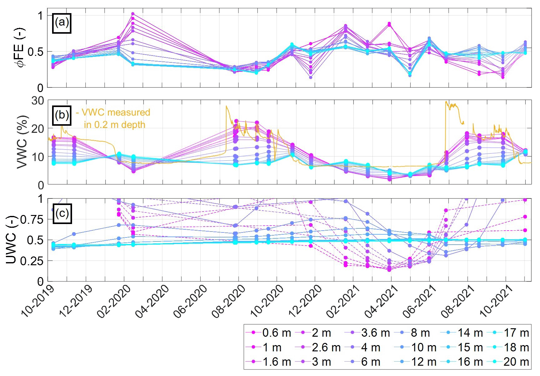
Figure 11Temporal changes in (a) ϕFE. (b) Measured and estimated volumetric water content (VWC) and (c) unfrozen water content (UWC) at the borehole location at various depths (0.6–20 m). The cementation exponent was estimated for a given measurement of VWC (baseline date in October 2019) within the debris layer (Φ=0.6). Porosity, fluid resistivity (ρω=220 Ω m), cementation exponent (m=2.2), and saturation exponent (n=2) were kept constant over time, and VWC was calculated using Eqs. (7), (9), and (10). To obtain the UWC (Eq. 12), the parameter b was fitted for each depth according to the exponential behavior of the corresponding resistivity data at 0.5 Hz using Eq. (11) with ρ0=9.331 Ωm and °C.
4.3 Spatiotemporal variability in the phase frequency effect
Pogliotti et al. (2015) found a pronounced spatial variability in the active layer thickness at the two boreholes in Cervinia Cime Bianche (see Table 1) and argue that the difference can be related to contrasting water contents and varying surface and subsurface conditions in terms of weathering and fracturing of the bedrock. They suggest a higher ice content in the SBH compared to the DBH, which was further supported by PJI results of Mollaret et al. (2020), indicating ice contents of up to 10 % at the DBH and up to 17 % at the SBH. Additionally, our results show (see Fig. 4) an overall shallower uppermost layer in the northeast of the study site (1–2 m difference to southwest) with lower ρ′ at depth close to the DBH compared to the SBH.
While Fig. 8d demonstrates a clear relation of the ϕFE and the PJI-estimated ice content, and Fig. 11 shows consistent temporal changes in ϕFE at the borehole position, Fig. 12 evaluates the applicability of ϕFE for spatiotemporal changes across the entire imaging plane. Figure 13a shows the resolved ϕFE along the SIPM profile and the computed annual changes in ϕFE between August 2020 and August 2022, and Fig. 12c and d compare the ϕFE values at the borehole position with ground temperature readings of both boreholes. Both the distribution with depth, as well as the inter-annual differences, show a consistent pattern between ϕFE and borehole temperatures. At the borehole location, we observe, for all three dates, lower ϕFE (< 0.35) in the unfrozen active layer compared to zones at > 5 m depth related to the permafrost body, with ϕFE values ranging from 0.35 to 0.45. From numerical modeling (not shown), we found that an electrode separation of 3 m with dipole lengths of 3 and 12 m were small enough to delineate the transition between the thawed active layer and the permafrost using the ϕFE. Previous geophysical investigations along the ERT/RST monitoring profile in August 2017 report low seismic P-wave velocities of <1000 m s−1 and low electrical resistivities of <10 kΩ m within the uppermost 4–5 m thick layer and intermediate electrical resistivities (10–50 kΩ m) and high seismic velocities (2000–5000 m s−1) for the permafrost zone below (Mollaret et al., 2020). PJI results of the seismic and electrical data yielded ice contents of ∼ 15 % within the permafrost body at the SBH, where also the ϕFE shows high values. In accordance with borehole temperatures, Fig. 12a also reveals clearly lower ϕFE in the permafrost at depths between 8 and 15 m in 2020 (ϕFE≈0.36), compared to the colder year 2022, with ϕFE values in the range of 0.45 (see the yellow box in Fig. 12a). Hence, our results suggest that inter-annual temperature changes of ≈0.2 °C at depth can be resolved by the change of 0.05 in the ϕFE, implying a high sensitivity of SIPM to small changes in temperature that might not be resolved through ERT monitoring alone. Below 20 m, we assign low credibility to the ϕFE values due to large DOI values (i.e., > 0.2) and low sensitivity in the computed images.
The general tendency of ϕFE for the entire imaging plane of the SIPM profile is similar to that of the borehole location (Fig. 12a and d); however, the lateral heterogeneity is more pronounced than a vertically homogeneous pattern. In the northern part of the SIPM profile (i.e., between 0–30 m), with lowest ρ′ values and small ϕFE for all dates, also ϕFE changes are the smallest during the SIP monitoring period, with a slight decrease in ϕFE (ϕFE difference ) between August 2020 and August 2021 and an increase between 2021 and 2022 (ϕFE difference ∼ 0.1). Due to the low ϕFE and ρ′ values at all depths in the north of the study site (see, e.g., Fig. 4), we interpret this part of the monitoring profile as an area of low ice content. The highest ρ′ and ϕFE values are observed in the south between 140 and 189 m profile length, where the surface is dominated by the coarsest blocks within the study site. Here, we find a consistent increase in ϕFE over the 2 years, with positive ϕFE differences of ≈ 0.3 between 2020 and 2022 indicating a high change in the temperature/ice content within this part of the SIPM profile. Between profile meter 40 and 60, as well as between 90 and 115 m, two anomalies are resolved, characterized by inconsistent changes in the ϕFE during the SIP monitoring period. Such a ϕFE anomaly corresponds to high water content resolved from PJI (see Figs. 8, C1). Between 90 and 115 m, the surface cover is fine-grained and consists of silt, soil, and vegetation and revealed the highest water content, as well as small ρ′ and ϕFE values. While the permafrost body is generally assumed to be completely frozen for consecutive years with only small ice content changes at depth, strong spatiotemporal dynamics in the ϕFE at depth need to be considered with caution, as the data are inverted independently for measurements at different frequencies and time lapses and, thus, may be subject to uncertainties associated with inversions with different regularization, sensitivity, and contrasts. Such uncertainties could be reduced by the simultaneous inversion of SIP data measured over a range of frequencies (e.g., Günther and Martin, 2016; Kemna et al., 2014b; Son et al., 2007) and the inclusion of a spatiotemporal constraint. Yet, the small changes in temperature (0.2 K) observed in the borehole demonstrate that there is a change at depth, which seems to be captured with the ϕFE. Whether the magnitude of the ϕFE is biased by the smoothness constraint inversion is something that needs to be further explored in future studies.
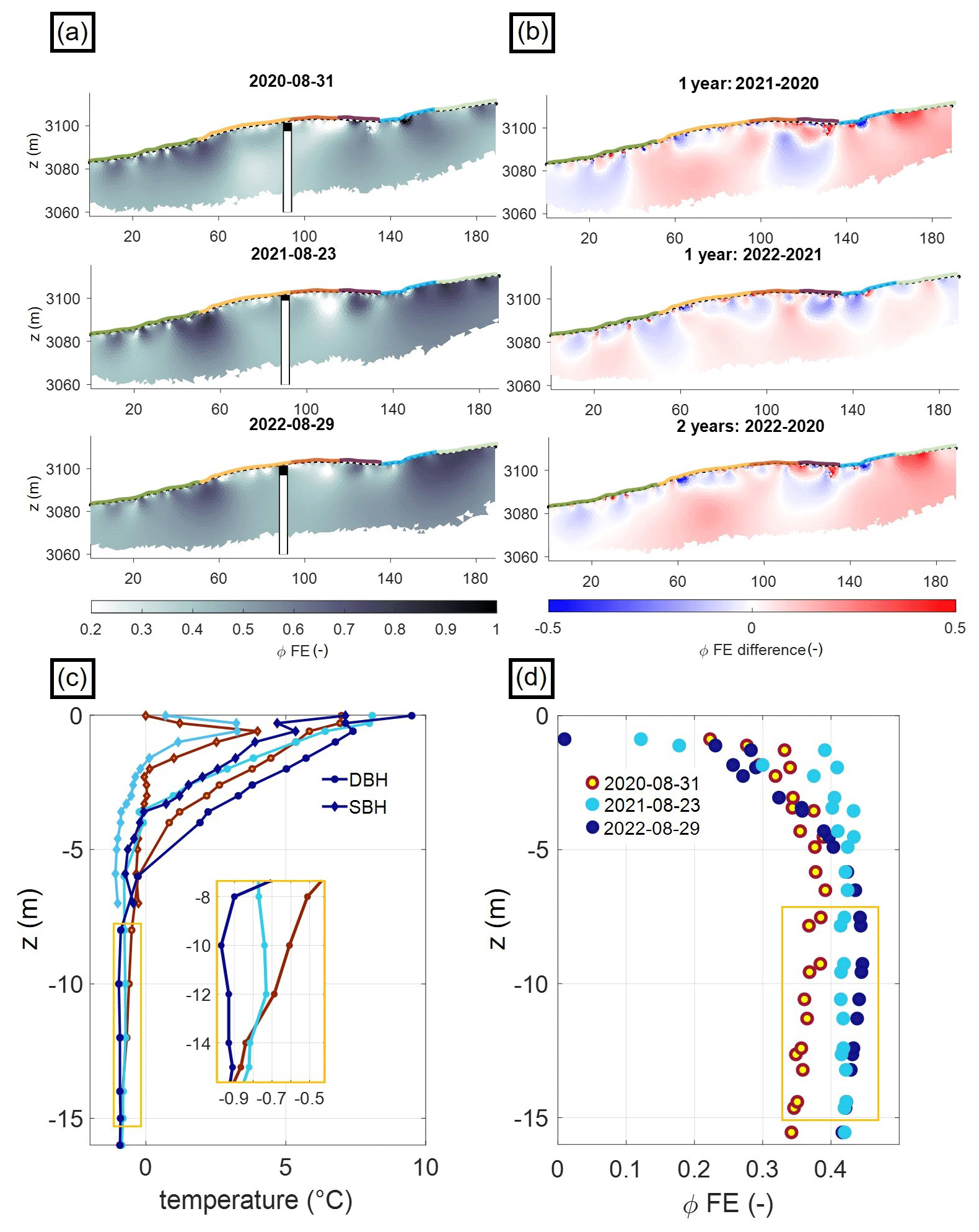
Figure 12(a) The phase frequency effect (ϕFE) and (b) the difference in ϕFE (i.e., ϕFE difference =ϕFE Aug22 – ϕFE Aug20) is visualized between August 2020 and August 2022 for the entire imaging plane (borehole position and thaw depths are highlighted). (c) Borehole temperature data of SBH and DBH and the (d) ϕFE extracted at the borehole position for the dates of the respective SIP measurements.
4.4 Comparison of the phase frequency effect and PJI ice and water content estimations
Our analysis, based on field and laboratory data, suggests that temperature, water, and ice content are dominant factors controlling the frequency dependence of the SIP data throughout the freeze–thaw transition. Ice content has not been directly quantified at the study area, hindering a direct comparison between ϕFE and this key parameter. The only information about the ice content at the site has been presented by Mollaret et al. (2020) through a PJI of the data collected in the ERT/RST profile. We have seen that at the borehole location (see Fig. 8), ϕFE and PJI-estimated ice content are strongly correlated. In this regard, the ϕFE could be an initial way to incorporate SIP information into the 4PM and improve the estimation of ice content in the PJI.
Figure 13 evaluates the correlation between the ϕFE and the ice and water contents estimated from the PJI for selected zones of interest (ZOIs) in different parts of the tomogram and for depths representative of the active layer and the permafrost body. The results show that a specific relationship, such as observed at the borehole location, is not observed in all regions of the tomogram. High ϕFE values in the permafrost body mostly coincide with high ice contents and low water contents, and vice versa; however, it is not observed in all ZOIs, for instance, in ZOI4 linked to fine-grained surface material. Additionally, ϕFE fluctuations within the active layer are high, and ϕFE values are in the range of the permafrost body for some of these ZOIs in the active layer. Such variations in the active layer could be minimized in the future by regularization strategies like, for example, the minimal gradient support (Blascheck et al., 2008), which permits us to solve for sharp contrasts between interfaces, and still ensure smooth variations within the different zones. Also, further studies should investigate the regularizations across time and space dimensions to enhance the consistency between the resolved electrical models and improve the quantitative meaning of the ϕFE
Differences observed in Fig. 13 between the ϕFE and PJI-derived ice contents at depth might indicate that ice contents might be overestimated in some areas due to the anisotropic smoothness constraint inversion or the insensitivity of RST and ERT to possible fractures so that lateral changes in ice content are not resolved. As mentioned above, the PJI is strongly controlled by the porosity model defined as a start model for the inversion (see, e.g., Steiner et al., 2021, for a discussion), and the gradient model forces a lateral smoothness in the parameters, which might not be present at the site. Such lateral variations will be better resolved in the SIP imaging and likely better retrieved in the frequency dependence. Additionally, Maierhofer et al. (2022) demonstrated that surface conduction changes spatially, with a large polarization (σ′′) associated with ice-rich areas (even at low frequencies due to EDL polarization at the ice–water interface). In addition, our results (see Figs. 5 and 9) reveal temporal and spatial changes in surface conductivity, with ρ′′ and ϕ changing across different positions of the profile (geological changes) and different seasons. The inclusion of a constant value for the surface conduction improves the overall ice content estimations based on the PJI (e.g., Mollaret et al., 2020); yet, the chosen value is only representative of pure ice, where variations due to a mixture of ice, sediment, and rock are ignored. To obtain reliable petrophysical parameters based on a PJI, the spatially and temporally varying surface conduction, as observed in our SIP results, needs to be considered additionally.
The occurrence of non-zero ice content estimates in regions where they are unlikely, such as in areas where temperatures are positive, shows an over-estimation of the ice content in the active layer through the PJI. Similar observations have been made by Pellet et al. (2016) and Wagner et al. (2019), who proposed and implemented physical constraints on water content (based on soil moisture measurements) or temperature-dependent constraints on ice occurrence during inversion. However, such ice constraints are limited to sparsely distributed point locations and might bias the constraints used in the inversions for those areas without information. Figure 13 shows that the minimal fi is about 10 %, even for the ZOIs retrieved from the AL. This problem can be resolved by fixing a spatial constraint with an ice content of 0 % in the active layer, yet such an inversion would require exact information about the geometry of the active layer.
The quantitative interpretation of ϕFE is likely still open to debate; however, its applicability is supported in our study through the analysis of independent measurements in well-controlled experiments conducted in the laboratory (Figs. 6 and 7). These analyses reveal a clear distinction in the polarization response between unfrozen and frozen states and a significant frequency dependence in the absolute ϕ values with decreasing temperature, which in turn is related to the well-known temperature-dependent relaxation behavior of ice (Auty and Cole, 1952), with the full spectrum presented in the Appendix B. Laboratory and field results reveal that between 5 and 8 Hz an inflection point between the low-polarization response at low frequencies associated with the polarization of grain–water interfaces and the increase in the response at high frequencies exist due to the polarization of ice. Such an inflection point depends on the texture of the rock, as well as the ice content (and temperature), as evidenced in our laboratory measurements. Additionally, at temperatures < 0 °C, a higher increase in absolute ϕ values for the loose-sediment sample and the debris compared to the solid-rock sample and the bedrock suggests a correlation of ϕ with ice. Even though a similar behavior in the polarization during freezing and thawing cycles is observed for laboratory and field data, the increase in the absolute phase is smaller for laboratory data (as shown for Fig. 7). The discrepancy between laboratory and field data sets can be related to larger heterogeneities (according to Fig. 5a) and variations in the volumes of investigation at the field scale, as well as different sources of contamination in the data such as electromagnetic coupling effects, which can be reduced to a minimum within the laboratory. Additionally, we observe large contrasts along the SIP monitoring profile with large variations due to changes in porosity, water, and ice contents. These changes play a big role in the inversion of the field data, especially when inverted at different frequencies. Hence, future investigations should consider investigating the influence of small heterogeneities within the debris layer using small electrode spacings. We also note here that the ϕFE needs to be analyzed for measurements at other sites, corresponding to different lithology, porosity, and ice content. Moreover, other polarization processes occurring at higher frequencies, for example, related to high clay content, metallic minerals, or peat within the subsurface, would also influence the ϕFE and need to be addressed in future studies. In this regard, the ϕFE offers qualitative information about the geometry and temporal changes in areas rich in ice. Further studies might attempt to include such information – at least as a spatial constraint – within the PJI.
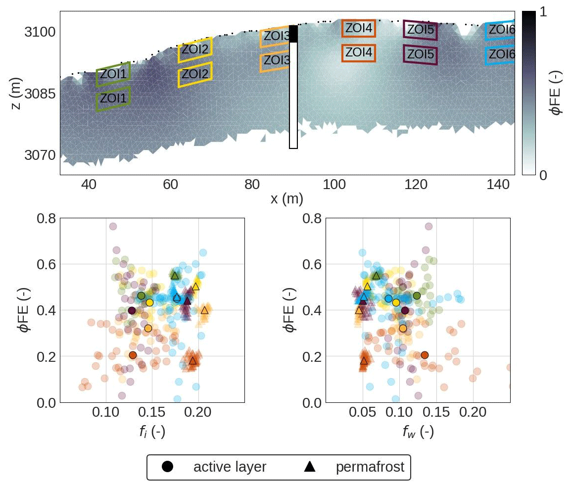
Figure 13Correlation between PJI-derived ice and water content estimates and the phase frequency effect for selected zones of interest (ZOIs) within the active layer and the permafrost body along the SIP monitoring profile.
Additional investigations are needed to find petrophysical models linking SIP parameters and ice content (e.g., Zorin and Ageev, 2017), where the ϕFE could be another option. Such a model could explicitly account for surface conduction and thereby help to reduce the uncertainty in the PJI inversion. However, to that end, further SIP measurements at different sites and ice content are required (Maierhofer et al., 2021).
In this study, we presented time-lapse SIP imaging data collected at a mountain permafrost site during a measurement period of 3 years. The data were obtained in the frequency domain between 0.1–75 Hz using a combination of dipole–dipole normal and reciprocal and multiple gradient protocols. Our analysis highlights clear seasonal changes in the complex resistivity images for all frequencies, with an increase in late autumn and a decrease in early summer and most prominent changes at shallow depths in the active layer. Characteristic changes in polarization can be attributed either to the freezing period in autumn (September–November), before a permanent snow cover has been established, or to subsurface thawing processes in late spring and early summer (June–July), when melting snow and rain lead to a decrease in phase values. During winter, complex resistivity values increase to their maximum for all frequencies and depths, which can partly be explained by the high resistance leading to an increase in phase errors and data uncertainty. This is demonstrated within electric circuit tests in the laboratory to assess the effect of a high sample resistance and electromagnetic fields (i.e., parasitic capacitive coupling) on SIP measurements and examine the lower bound of the error level of the phase measurements to be expected in the field.
Complex resistivity–temperature relationships at the borehole location show a linear dependency for positive temperatures and an exponential relation for subzero temperatures with different amplitudes for different substrates (debris and bedrock). Clear hysteresis effects are observed in the freeze–thaw transition processes relating the change in polarization signals to a difference in water content for these phase changes. Supercooling effects are observed through lower complex resistivity values during freezing than during thawing, which is due to higher unfrozen water contents during freezing compared to thawing processes at the same temperature. This interpretation is confirmed by laboratory measurements on rock samples from the site, which, upon freezing and thawing, exhibit an absolute phase increase with decreasing temperature at higher frequencies, with the general spectral behavior being consistent with the known polarization properties of ice.
Our analysis based on field and laboratory freeze–thaw cycles, as well as on spatial patterns of the SIP behavior in freezing conditions, suggests that temperature, water, and ice content are dominant factors controlling the polarization at the frequencies measured in this study. Considering that field SIP devices are often limited in the frequency range and might lack the possibility of recovering the frequency of the polarization maximum (in our case, the full process of ice relaxation) required to fit a dispersion model such as the Cole–Cole model, this study focuses on the investigation of the phase frequency effect, exploiting the spectral information gained through SIP field measurements in a frequency range between 0.1–75 Hz. Yet, it is important that the frequency range in the SIP data extends above a sensitive frequency which corresponds to an inflection point between the low-polarization values (due to the polarization of rock–water interface) and the high values associated with the polarization of ice. We propose the resistivity phase frequency effect (ϕFE) as a proxy to discriminate between regions with no ice and regions richer in ice (i.e., also to discriminate temporal changes in ice content). Laboratory and field data show a clear exponential increase in the temperature dependence of the ϕFE during freezing and higher amplitudes for higher ice contents (i.e., in the pores of the sediment sample and within the debris layer). Inter-annual changes in the ϕFE at the field scale are spatially heterogeneous, which is interpreted to be related to varying surface/subsurface conditions, temperature changes, and ice and water contents along the monitoring profile. Small changes in temperature at depth can be resolved by SIP through examining changes in the ϕFE.
When comparing the phase frequency effect with ice content estimates from electric and seismic data sets using the petrophysical joint inversion scheme (PJI), we observe a high consistency at the borehole location but do not obtain the same relationship for the entire imaging plane. These inconsistencies highlight the difficulty of obtaining ice content data sets for validation, as also PJI-derived ice content estimates are based on various assumptions within the petrophysical model with inherent uncertainties. Future investigations should focus on the integration of IP data in the PJI approach as structural constraints or as an additional parameter in the underlying petrophysical model for an improved estimation of the ice content with applications in different permafrost landforms. In the presence of ice within the subsurface, polarization increases, and thus spatially and temporally varying surface conduction has to be considered additionally to electrolytic conduction within the PJI to obtain reliable petrophysical parameters. Thus, further investigations are needed to find a petrophysical model linking IP and ice content, such as a combination of the phase frequency effect with additional laboratory studies required to link the phase frequency effect with ice contents.
In Table A1, we present the measurement setup for SIP data collected along the monitoring profile between October 2019 and October 2022 and additional filtering parameters.
Table A1Filtering of SIP time-lapse data–monitoring setup (electrode configuration and frequency range) and remaining quadrupoles after filtering for each measuring date. N&R stands for normal and reciprocal.
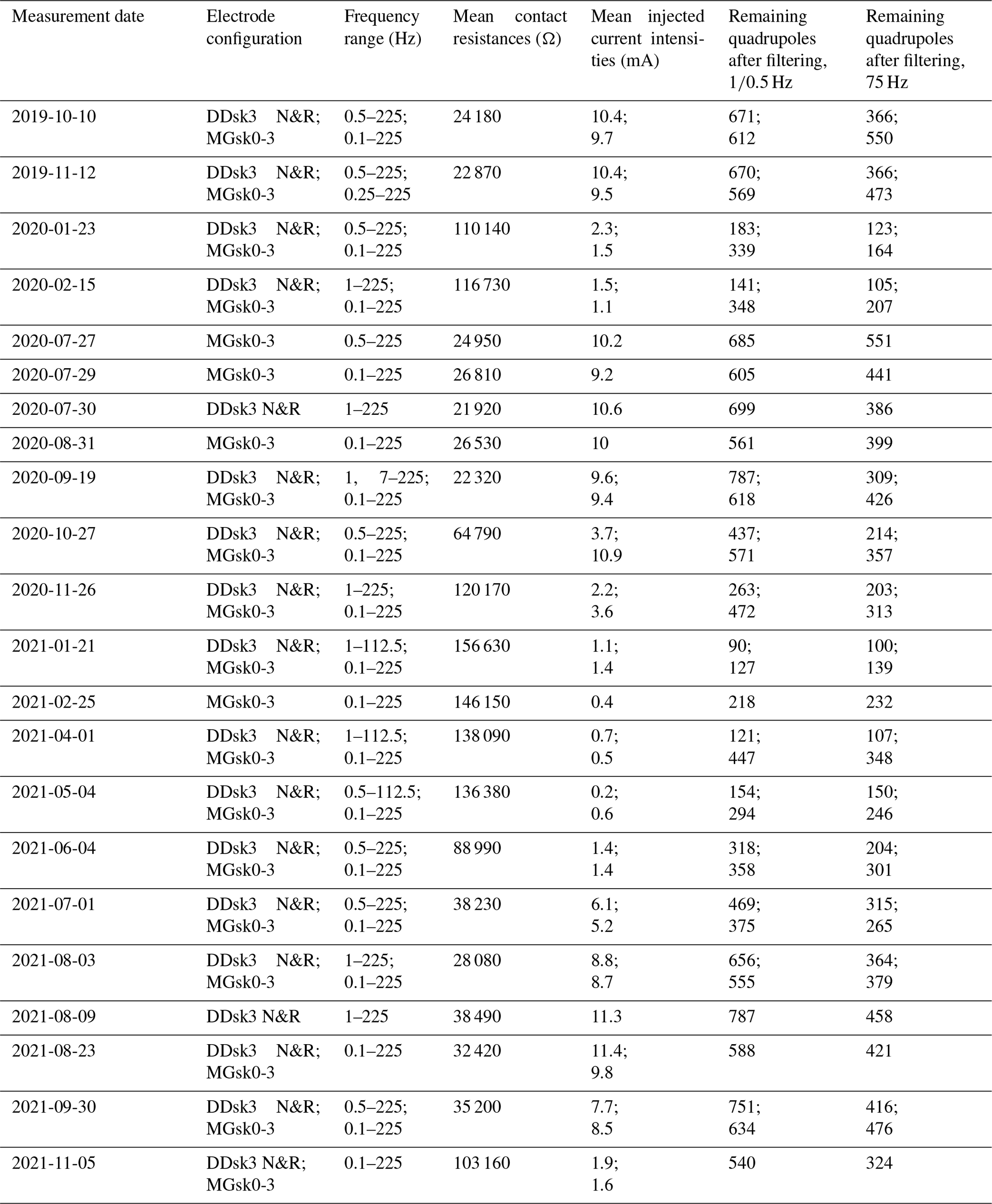
In Fig. B1, we show laboratory measurements performed on a cylindrical solid-rock sample of 10 cm length and 3 cm diameter of amphibolite (with a porosity of 3.5 %) and a loose-sediment surface sample, both collected close to the SIP monitoring profile. The electrical impedance was measured in a frequency range of 10 mHz to 45 kHz during controlled freeze–thaw cycles (+20 to −40 to +20 °C).
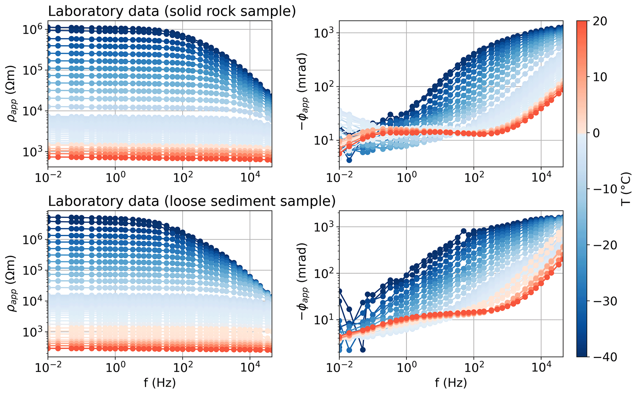
Figure B1Broadband SIP laboratory measurements on a solid-rock sample and a loose-sediment sample collected at the site close to the monitoring profile. Apparent resistivity and phase values are shown in a frequency range between 10 mHz and 45 kHz during controlled freeze–thaw cycles (+20 to −40 to +20 °C).
In Fig. C1, we show PJI results for seismic travel times and electrical resistivity measurements collected along the SIP monitoring profile. Differing velocities can be observed between the debris and bedrock, with the lowest velocities occurring in the near-surface within the porous debris layer, ranging from roughly 500 to 1500 m s−1 and corresponding to a high air content. Maximum rock contents with a porosity of ∼ 20 % and minimum rock contents reaching a porosity of 70 % are encountered in the bedrock and surface debris layer, respectively. Accordingly, the transition between debris and bedrock at the borehole location was estimated at a depth of 1.2 m by calculating the inflection point in the rock content at the borehole position.
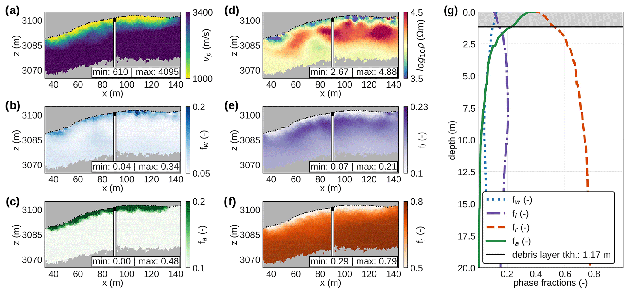
Figure C1Petrophysical joint inversion results for August 2020. (a–f) Imaging results in terms of geophysical parameters, i.e., the seismic P-wave velocity (vp) and electrical resistivity (ρ), and petrophysical parameters, i.e., the ice, water, air, and rock contents resolved through the petrophysical joint inversion. (g) Virtual 1D logs extracted from the imaging results at the borehole location and estimated debris layer thickness.
The complex resistivity data were fitted for each frequency using a linear model for positive temperatures and an exponential model for subzero temperatures according to
with the coefficients for different frequencies for debris and bedrock summarized in Table D1.
Table D1Coefficients for complex resistivity with temperature fits for two frequencies (0.5 and 75 Hz) and for two material compositions (debris and bedrock).
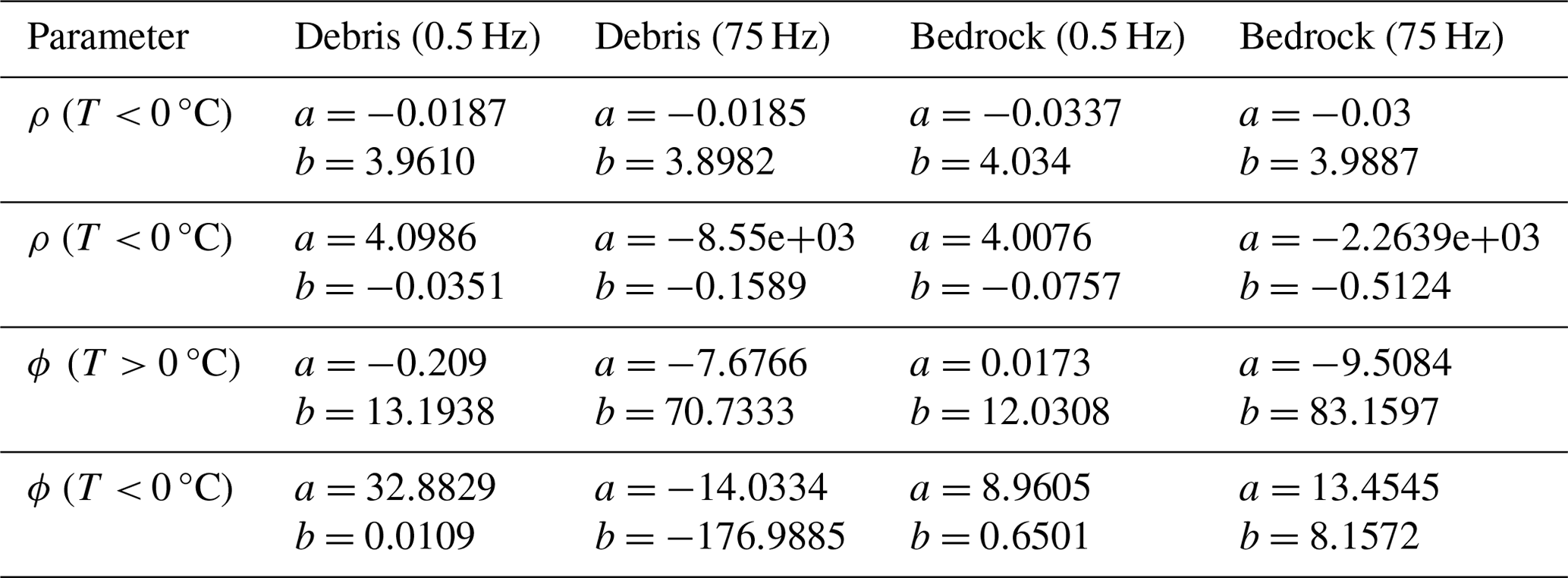
To quantitatively assess the effect of a high sample resistance and PCC on SIP measurements and examine the accuracy of the DAS-1 measurement device in our SIP monitoring measurements, we built an electric circuit using commercial resistors and capacitors with known values (see Fig. E1) and performed measurements with the DAS-1 field device and the Portable Spectral Induced Polarization (PSIP) laboratory unit (Ontash & Ermac Inc., NJ, USA). Coaxial cables were used to connect the circuit and instrument ports to reduce cross-talking, similar to field conditions. We first collected impedance measurements on a resistor network with varying resistances from 10 Ω to 15 kΩ (Fig. 11a). For the PSIP instrument we observe high accuracy for both magnitude and phase measurements, where the measured values confirm the theoretical response for all resistors. The SIP field instrument proves high accuracy from 0.1 to 75 Hz for resistances up to 1 kΩ, which demonstrates that the coupling effects of the device and the cables can be neglected. If R exceeds 1 kΩ, the magnitude of the impedance is underestimated, and the phase response increases with frequency due to the capacitive load of the amplifiers similar to Zimmerman et al. (2008). Above 100 Hz, phase errors of 10 mrad occur, whereas before these measurement frequencies were not considered in our SIP monitoring analysis. In Fig. 11b, we show impedance measurements of the PSIP and DAS-1 devices of a known resistance in parallel to a known capacitance. At low frequencies and resistances, both devices show phase errors smaller than 0.5 %. At frequencies above 100 Hz, phase values strongly deviate from the theoretical response. For measurements above 10 Hz, a sudden decrease in the phase values leads to an underestimation of the theoretical response of the DAS-1 measurements, which is consistently observed for all measurements. Yet, the phase frequency effect is still a stable measure, with phase frequency errors smaller than 4 % for resistances < 1kΩ for the laboratory and the field devices.
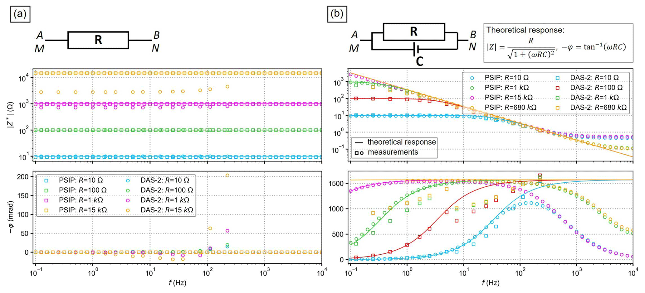
Figure E1Test of the phase accuracy of the SIP measurement device used in our field surveys. We show the measured (with the PSIP lab device and the DAS-1 field device) and calculated the magnitude and phase response of a resistor network with varying resistances (a) and for a known resistance in parallel to a known capacitance (C=470 µF) (b).
The borehole temperature data from the ARPA office, as well as the SIP field and laboratory data that support the findings of this study, are available from the corresponding author upon request.
TM, AFO, and CHa designed the experimental setup. TM, ED, UMD, and AFO planned and coordinated the field logistics of the installation and conduction of the monitoring measurements. ED and UMD provided further background information on the site. TM, AFO, and NR processed the geophysical field data, and CM helped with the preparation of a figure. JL and AK collected and processed the laboratory data. AFO, CHa, CHi, and TM interpreted the geophysical signatures. CHa, AFO, NR, CHi, AK, JL, and TM discussed the results. TM led the preparation of the draft and wrote the major part of the text with the essential help of CHa, AFO, and CHi, while all authors contributed actively to the intermediate and final version of the paper.
At least one of the (co-)authors is a member of the editorial board of The Cryosphere. The peer-review process was guided by an independent editor, and the authors also have no other competing interests to declare.
Publisher’s note: Copernicus Publications remains neutral with regard to jurisdictional claims made in the text, published maps, institutional affiliations, or any other geographical representation in this paper. While Copernicus Publications makes every effort to include appropriate place names, the final responsibility lies with the authors.
This study has been supported by the Swiss National Science Foundation (SNSF) (project no. 200021L_1788236) and the German Research Foundation (DFG) (project no. 403089687). We are, furthermore, thankful to the ARPA office for providing the borehole temperature data and ARPA, as well as the cable car company Cervino Spa for the logistical support of our research activities at the Cervinia Cime Bianche field site. We also thank Michel Isabellon, Lukas Aigner, Paolo Pogliotti, Doris Schlögelhofer, Alberto Carrera, Walter Loderer, and Sarah Morard for their help in the preparation of the equipment, the installation of the geophysical monitoring profile, and the collection of the geophysical monitoring data.
This research has been supported by the Swiss National Science Foundation (SNSF) (project no. 200021L_1788236).
This paper was edited by Ylva Sjöberg and reviewed by Matthias Bücker and one anonymous referee.
Auty, R. P. and Cole, R. H.: Dielectric properties of ice and solid D2O, J. Chem. Phys., 20, 1309–1314, https://doi.org/10.1063/1.1700726, 1952.
Bazin, S., Lysdahl, A., Olaus Harstad, A., and Frauenfelder, R.: Resistivity and Induced Polarization (ERT/IP) survey for bedrock mapping in Permafrost, Svalbard, 25th Eur. Meet. Environ. Eng. Geophys. Held Near Surf. Geosci. Conf. Exhib. 2019, NSG 2019, The Hague, The Netherlands, 8–12 September 2019, 1–5, https://doi.org/10.3997/2214-4609.201902362, 2019.
Binley, A. and Kemna, A.: DC Resistivity and Induced Polarization Methods, in: Hydrogeophysics, Water Science and Technology Library book series, edited by: Rubin, Y. and Hubbard, S. S., volume 50, 129–156, https://doi.org/10.1007/1-4020-3102-5_5, 2005.
Binley, A. and Slater, L.: Resistivity and Induced Polarization: theory and Applications to the Near-Surface Earth, Cambridge, United Kingdom, New York, USA, New Delhi, India, ISBN 9781108685955, https://doi.org/10.1017/9781108685955, 2020.
Binley, A., Slater, L. D., Fukes, M., and Cassiani, G.: Relationship between spectral induced polarization and hydraulic properties of saturated and unsaturated sandstone, Water Resour. Res., 41, W12417, https://doi.org/10.1029/2005WR004202, 2005.
Binley, A., Kruschwitz, S., Lesmes, D., and Kettridge, N.: Exploiting the temperature effects on low frequency electrical spectra of sandstone: A comparison of effective diffusion path lengths, Geophysics, 75, 10–13, https://doi.org/10.1190/1.3483815, 2010.
Biskaborn, B. K., Smith, S. L., Noetzli, J., Matthes, H., Vieira, G., Streletskiy, D. A., Schoeneich, P., Romanovsky, V. E., Lewkowicz, A. G., Abramov, A., Allard, M., Boike, J., Cable, W. L., Christiansen, H. H., Delaloye, R., Diekmann, B., Drozdov, D., Etzelmüller, B., Grosse, G., Guglielmin, M., Ingeman-Nielsen, T., Isaksen, K., Ishikawa, M., Johansson, M., Johannsson, H., Joo, A., Kaverin, D., Kholodov, A., Konstantinov, P., Kröger, T., Lambiel, C., Lanckman, J. P., Luo, D., Malkova, G., Meiklejohn, I., Moskalenko, N., Oliva, M., Phillips, M., Ramos, M., Sannel, A. B. K., Sergeev, D., Seybold, C., Skryabin, P., Vasiliev, A., Wu, Q., Yoshikawa, K., Zheleznyak, M., and Lantuit, H.: Permafrost is warming at a global scale, Nat. Commun., 10, 264, https://doi.org/10.1038/s41467-018-08240-4, 2019.
Bittelli, M., Flury, M., and Roth, K.: Use of dielectric spectroscopy to estimate ice content in frozen porous media, Water Resour. Res., 40, W04212, https://doi.org/10.1029/2003WR002343, 2004.
Blaschek, R., Hördt, A., and Kemna, A.: A new sensitivity-controlled focusing regularization scheme for the inversion of induced polarization data based on the minimum gradient support, Geophysics, 73, F45–F54, https://doi.org/10.1190/1.2824820, 2008.
Bullemer, B. and Riehl, N.: Bulk and Surface Conductivity of Ice, Solid State Commun., 4, 447–448, https://doi.org/10.1016/0038-1098(66)90325-5, 1996.
Caranti, J. M. and Illingworth, A. J.: Frequency Dependence of the Surface Conductivity of Ice, J. Phys. Chem., 87, 4078–4083, https://doi.org/10.1021/j100244a016, 1983.
Cole, K. S. and Cole, R. H.: Dispersion and absorption in dielectrics I. Alternating current characteristics, J. Chem. Phys., 9, 341–351, https://doi.org/10.1063/1.1750906, 1941.
Coperey, A., Revil, A., Abdulsamad, F., Stutz, B., Duvillard, P. A., and Ravanel, L.: Low-Frequency Induced Polarization of Porous Media Undergoing Freezing: Preliminary Observations and Modeling, J. Geophys. Res.-Sol. Ea., 124, 4523–4544, https://doi.org/10.1029/2018JB017015, 2019.
Dahlin, T. and Zhou, B.: Multiple-gradient array measurements for multi-channel 2D resistivity imaging, Near Surf. Geophys, 4, 113–123, 2006.
Daniels, J. J., Keller, G. V., and Jacobson, J. J.: Computer-assisted interpretation of electromagnetic soundings over a permafrost section, Geophysics, 41, 752–765, https://doi.org/10.1190/1.1440647, 1976.
Dash, J. G., Rempel, A. W., and Wettlaufer, J. S.: The physics of premelted ice and its geophysical consequences, Rev. Mod. Phys., 78, 695–741, https://doi.org/10.1103/RevModPhys.78.695, 2006.
Doetsch, J., Ingeman-Nielsen, T., Christiansen, A. V., Fiandaca, G., Auken, E., and Elberling, B.: Direct current (DC) resistivity and induced polarization (IP) monitoring of active layer dynamics at high temporal resolution, Cold Reg. Sci. Technol., 119, 16–28, https://doi.org/10.1016/j.coldregions.2015.07.002, 2015.
Duvillard, P., Magnin, F., Revil, A., Legay, A., Ravanel, L., Abdulsamad, F., and Coperey, A.: Temperature distribution in a permafrost-affected rock ridge from conductivity and induced polarization tomography, Geophys. J. Int., 225, 1207–1221, https://doi.org/10.1093/gji/ggaa597, 2021.
Duvillard, P. A., Revil, A., Qi, Y., Soueid Ahmed, A., Coperey, A., and Ravanel, L.: Three-Dimensional Electrical Conductivity and Induced Polarization Tomography of a Rock Glacier, J. Geophys. Res.-Sol. Ea., 123, 9528–9554, https://doi.org/10.1029/2018JB015965, 2018.
Etzelmüller, B., Guglielmin, M., Hauck, C., Hilbich, C., Hoelzle, M., Isaksen, K., Noetzli, J., Oliva, M., and Ramos, M.: Twenty years of European mountain permafrost dynamics – the PACE legacy, Environ. Res. Lett., 15, 10, https://doi.org/10.1088/1748-9326/abae9d, 2020.
Flores Orozco, A., Williams, K. H., Long, P. E., Hubbard, S. S., and Kemna, A.: Using complex resistivity imaging to infer biogeochemical processes associated with bioremediation of an uranium-contaminated aquifer, J. Geophys. Res.-Biogeo., 116, G03001, https://doi.org/10.1029/2010JG001591, 2011.
Flores Orozco, A., Kemna, A., and Zimmermann, E.: Data error quantification in spectral induced polarization imaging, Geophysics, 77, E227–E237, https://doi.org/10.1190/geo2010-0194.1, 2012.
Flores Orozco, A., Williams, K. H., and Kemna, A.: Timelapse spectral induced polarization imaging of stimulated uranium bioremediation, Near Surf. Geophys., 11, 531–544, https://doi.org/10.3997/1873-0604.2013020, 2013.
Flores Orozco, A., Bücker, M., Steiner, M., and Malet, J.-P.: Complex-conductivity imaging for the understanding of landslide architecture, Eng. Geol., 243, 241–252, https://doi.org/10.1016/j.enggeo.2018.07.009, 2018.
Flores Orozco, A., Kemna, A., Binley, A., and Cassiani, G.: Analysis of time-lapse data error in complex conductivity imaging to alleviate anthropogenic noise for site characterization, Geophysics, 84, B181–B193, https://doi.org/10.1190/GEO2017-0755.1, 2019.
Frolov, A. D.: Elastic and electrical properties of frozen ground, in: Proceedings at 2nd International Conference on Permafrost (USSR contribution), edited by: Sanger and Hyde, H., National Academy of Sciences, Washington DC, 307–312, 1973.
Glover, P.: What is the cementation exponent? A new interpretation, Leading Edge, 28, 82–85, https://doi.org/10.1190/1.3064150, 2009.
Grimm, R. E. and Stillman, D. E.: Field test of detection and characterisation of subsurface ice using broadband spectral induced polarisation, Permafrost Periglac., 26, 28–38, https://doi.org/10.1002/ppp.1833, 2015.
Guglielmin, M. and Vannuzzo, C.: Studio della distribuzione del permafrost e delle relazioni con i ghiacciai della piccola età glaciale nell'alta valtournenche (Valle d'Aosta, Italia), Atti Ticinesi di Scienze della Terra, 38, 119–127, 1995.
Günther, T. and Martin, T.: Spectral two-dimensional inversion of frequency-domain induced polarization data from a mining slag heap, J. Appl. Geophys., 135, 436–448, https://doi.org/10.1016/j.jappgeo.2016.01.008, 2016.
Harris, C., Haeberli, W., Vonder Mühll, D., and King, L.: Permafrost monitoring in the high mountains of Europe: the PACE Project in its global context, Permafrost Periglac., 12, 3–11, https://doi.org/10.1002/ppp.377, 2001.
Hauck, C.: Frozen ground monitoring using DC resistivity tomography, Geophys. Res. Lett., 29, 10–13, https://doi.org/10.1029/2002GL014995, 2002.
Hauck, C.: New Concepts in Geophysical Surveying and Data Interpretation for Permafrost Terrain, Permafrost Periglac., 137, 131–137, https://doi.org/10.1002/ppp.1774, 2013.
Hauck, C. and Kneisel, C.: Applied geophysics in periglacial environments, Cambridge University Press, 256 pp., ISBN 9780511535628, https://doi.org/10.1017/CBO9780511535628, 2008.
Hauck, C., Böttcher, M., and Maurer, H.: A new model for estimating subsurface ice content based on combined electrical and seismic data sets, The Cryosphere, 5, 453–468, https://doi.org/10.5194/tc-5-453-2011, 2011.
Hausmann, H., Krainer, K., Brückl, E., and Mostler, W.: Internal structure and ice content of Reichenkar rock glacier (Stubai Alps, Austria) assessed by geophysical investigations, Permafrost Periglac., 18, 351–367, https://doi.org/10.1002/ppp.601, 2007.
Harrington, J. S., Mozil, A., Hayashi, M., and Bentley, L. R.: Groundwater flow and storage processes in an inactive rock glacier, Hydrol. Process., 32, 3070–3088, https://doi.org/10.1002/hyp.13248, 2018.
Hilbich, C.: Time-lapse refraction seismic tomography for the detection of ground ice degradation, The Cryosphere, 4, 243–259, https://doi.org/10.5194/tc-4-243-2010, 2010.
Hilbich, C., Hauck, C., Hoelzle, M., Scherler, M., Schudel, L., Völksch, I., Vonder Mühll, D., and Mäusbacher, R.: Monitoring mountain permafrost evolution using electrical resistivity tomography: A 7-year study of seasonal, annual, and long-term variations at Schilthorn, Swiss Alps, J. Geophys. Res.-Earth, 113, F01S90, https://doi.org/10.1029/2007JF000799, 2008.
Hilbich, C., Fuss, C., and Hauck, C.: Automated time-lapse ERT for improved process analysis and monitoring of frozen ground, Permafrost Periglac., 22, 306–319, https://doi.org/10.1002/ppp.732, 2011.
Hilbich, C., Hauck, C., Mollaret, C., Wainstein, P., and Arenson, L. U.: Towards accurate quantification of ice content in permafrost of the Central Andes – Part 1: Geophysics-based estimates from three different regions, The Cryosphere, 16, 1845–1872, https://doi.org/10.5194/tc-16-1845-2022, 2022.
Hobbs, P. V.: Ice Physics, Clarendon, Oxford, 837 pp., ISBN 978-0-19-958771-1, 1974.
Huisman, J. A., Zimmermann, E., Esser, O., Haegel, F. H., Treichel, A., and Vereecken, H.: Evaluation of a novel correction procedure to remove electrode impedance effects from broadband SIP measurements, J. Appl. Geophys., 135, 466–473, https://doi.org/10.1016/j.jappgeo.2015.11.008, 2016.
Ingeman-Nielsen, T.: The effect of electrode contact resistance and capacitive coupling on complex resistivity measurements, SEG Technical Program Expanded Abstracts, 1376–1380, https://doi.org/10.1190/1.2369776, 2006.
Isaksen, K., Ødegård, R. S., Etzelmüller, B., Hilbich, C., Hauck, C., Farbrot, H., Eiken, T., Hygen, H. O., and Hipp, T.: degrading mountain permafrost in southern Norway: spatial and temporal variability of mean ground temperatures, 1999–2009, Permafrost Periglac., 22, 361–377, 2011.
Kemna, A.: Tomographic inversion of complex resistivity: Theory and application, PhD thesis, Ruhr-University of Bochum, ISBN 3-934366-92-9, 2000.
Kemna, A., Binley, A., Cassiani, G., Niederleithinger, E., Revil, A., Slater, L., Williams, K. H., Orozco, A. F., Haegel, F. H., Hördt, A., Kruschwitz, S., Leroux, V., Titov, K., and Zimmermann, E.: An overview of the spectral induced polarization method for near-surface applications, Near Surf. Geophys., 10, 453–468, https://doi.org/10.3997/1873-0604.2012027, 2012.
Kemna, A., Weigand, M., and Zimmermann, E.: Resistivity and SIP response of rocks during freezing and thawing, in: Proceedings of the 3rd International Workshop on Induced Polarization, Ile d'Oléron, France, 6–9 April 2014, https://ip.geosciences. mines-paristech.fr/s1_kemna (last access: 17 May 2022), 2014a.
Kemna, A., Huisman, J. A., Zimmermann, E., Martin, R., Zhao, Y., Treichel, A., Flores-Orozco, A., and Fechner, T.: Broadband Electrical Impedance Tomography for Subsurface Characterization Using Improved Corrections of Electromagnetic Coupling and Spectral Regularization, in: Tomography of the Earth's Crust: From Geophysical Sounding to Real-Time Monitoring, Springer, 1–20 https://doi.org/10.1007/978-3-319-04205-3_1, 2014b.
Keuschnig, M., Krautblatter, M., Hartmeyer, I., Fuss, C., and Schrott, L.: Automated Electrical Resistivity Tomography Testing for Early Warning in Unstable Permafrost Rock Walls Around Alpine Infrastructure, Permafr. Periglac., 28, 158–171, https://doi.org/10.1002/ppp.1916, 2017.
Krautblatter, M. and Hauck, C.: Electrical resistivity tomography monitoring of permafrost in solid rock walls, J. Geophys. Res., 112, F02S20, https://doi.org/10.1029/2006JF000546, 2007.
Krautblatter, M., Verleysdonk, S., Flores Orozco, A., and Kemna, A.: Temperature – calibrated imaging of seasonal changes in permafrost rock walls by quantitative electrical resistivity tomography (Zugspitze, German/Austrian Alps), J. Geophys. Res., 115, F02003, https://doi.org/10.1029/2008JF001209, 2010.
LaBrecque, D. J., Miletto, M., Daily, W., Ramirez, A., and Owen, E.: The effects of noise on Occam's inversion of resistivity tomography data, Geophysics, 61, 538–548, https://doi.org/10.1190/1.1443980, 1996.
Leroy, P., Revil, A., Kemna, A., Cosenza, P., and Ghorbani, A.: Complex conductivity of water-saturated packs of glass beads, J. Colloid Interface Sci., 321, 103–117, https://doi.org/10.1016/j.jcis.2007.12.031, 2008.
Lesmes, D. P. and Frye, K. M.: Influence of pore fluid chemistry on the complex conductivity and induced polarization responses of Berea sandstone, J. Geophys. Res.-Sol. Ea., 106, 4079–4090, 2001.
Lesparre, N., Nguyen, F., Kemna, A., Robert, T., Hermans, T., Daoudi, M., and Flores Orozco, A.: A new approach for time-lapse data weighting in electrical resistivity tomography, Geophysics, 82, E325–E333, https://doi.org/10.1190/GEO2017-0024.1, 2017.
Limbrock, J. K., Weigand, M., and Kemna, A.: Textural and mineralogical controls on temperature dependent SIP behavior during freezing and thawing, EGU General Assembly 2021, online, 19–30 April 2021, EGU21-14273, https://doi.org/10.5194/egusphere-egu21-14273, 2021.
Maierhofer, T., Hauck, C., Hilbich, C., and Flores-Orozco, A.: Spectral Induced Polarization Applied at Different Mountain Permafrost Sites in the European Alps, NSG2021 1st Conference on Hydrogeophysics, European Association of Geoscientists and Engineers, Bordeaux, France, 29 August–2 September 2021, 2021, 1–5, https://doi.org/10.3997/2214-4609.202120172, 2021.
Maierhofer, T., Hauck, C., Hilbich, C., Kemna, A., and Flores-Orozco, A.: Spectral induced polarization imaging to investigate an ice-rich mountain permafrost site in Switzerland, The Cryosphere, 16, 1903–1925, https://doi.org/10.5194/tc-16-1903-2022, 2022.
Mathys, T., Hilbich, C., Arenson, L. U., Wainstein, P. A., and Hauck, C.: Towards accurate quantification of ice content in permafrost of the Central Andes – Part 2: An upscaling strategy of geophysical measurements to the catchment scale at two study sites, The Cryosphere, 16, 2595–2615, https://doi.org/10.5194/tc-16-2595-2022, 2022.
McKenzie, J. M., Voss, C. I., and Siegel, D. I.: Groundwater flow with energy transport and water-ice phase change: Numerical simulations, benchmarks, and application to freezing in peat bogs, Adv. Water Resour., 30, 966–983, https://doi.org/10.1016/j.advwatres.2006.08.008, 2007.
Mollaret, C., Hilbich, C., Pellet, C., Flores-Orozco, A., Delaloye, R., and Hauck, C.: Mountain permafrost degradation documented through a network of permanent electrical resistivity tomography sites, The Cryosphere, 13, 2557–2578, https://doi.org/10.5194/tc-13-2557-2019, 2019.
Mollaret, C., Wagner, F. M., Hilbich, C., Scapozza, C., and Hauck, C.: Petrophysical Joint Inversion Applied to Alpine Permafrost Field Sites to Image Subsurface Ice, Water, Air, and Rock Contents, Front. Earth Sci., 8, 1–25, https://doi.org/10.3389/feart.2020.00085, 2020.
Mohammed, A. A., Kurylyk, B. L., Cey, E. E., and Hayashi, M.: Snowmelt infiltration and macropore flow in frozen soils: Overview, knowledge gaps, and a conceptual framework, Vadose Zone J., 17, 180084, https://doi.org/10.2136/vzj2018.04.0084, 2018.
Mudler, J., Hördt, A., Kreith, D., Sugand, M., Bazhin, K., Lebedeva, L., and Radić, T.: Broadband spectral induced polarization for the detection of Permafrost and an approach to ice content estimation – a case study from Yakutia, Russia, The Cryosphere, 16, 4727–4744, https://doi.org/10.5194/tc-16-4727-2022, 2022.
Oldenborger, G. A.: Subzero temperature dependence of electrical conductivity for permafrost geophysics, Cold Reg. Sci. Technol., 182, 103214, https://doi.org/10.1016/j.coldregions.2020.103214, 2021.
Oldenborger, G. A. and LeBlanc, A. M.: Monitoring changes in unfrozen water content with electrical resistivity surveys in cold continuous permafrost, Geophys. J. Int., 215, 965–977, https://doi.org/10.1093/GJI/GGY321, 2018.
Oldenburg, D. W. and Li, Y.: Estimating depth of investigation in DC resistivity and IP surveys, Geophysics, 64, 403–416, https://doi.org/10.1190/1.1444545, 1999.
Olhoeft, G. R.: Electrical properties of natural clay permafrost, Can. J. Earth Sci., 14, 16–24, 1977.
Parkhomenko, E. I.: Electrical Resistivity of Minerals and Rocks at High Temperature and Pressure, Rev. Geophys. Sp. Phys., 20, 193–218, 1982.
Pellet, C., Hilbich, C., Marmy, A., and Hauck, C.: Soil moisture data for the validation of permafrost models using direct and indirect measurement approaches at three alpine sites, Front. Earth Sci., 3, 91, https://doi.org/10.3389/feart.2015.00091, 2016.
Pelton, W. H., Rijo, L., and Swift Jr., C. M.: Inversion of two-dimensional resistivity and induced-polarization data, Geophysics, 43, 788-803, https://doi.org/10.1190/1.1440854, 1978.
Pepin, N., Bradley, R. S., Diaz, H. F., Baraer, M., Caceres, E. B., Forsythe, N., Fowler, H., Greenwood, G., Hashmi, M. Z., Liu, X. D., Miller, J. R., Ning, L., Ohmura, A., Palazzi, E., Rangwala, I., Schöner, W., Severskiy, I., Shahgedanova, M., Wang, M. B., Williamson, S. N., and Yang, D. Q.: Elevation-dependent warming in mountain regions of the world, Nat. Clim. Change, 5, 424–430, https://doi.org/10.1038/nclimate2563, 2015.
PERMOS: PERMOS Database, Swiss Permafrost Monitoring Network, Fribourg and Davos, Switzerland, PERMOS [data set], http://www.permos.ch/doi/permos-2021-01.html (last access: 17 May 2022), 2021.
Pogliotti, P., Guglielmin, M., Cremonese, E., Morra di Cella, U., Filippa, G., Pellet, C., and Hauck, C.: Warming permafrost and active layer variability at Cime Bianche, Western European Alps, The Cryosphere, 9, 647–661, https://doi.org/10.5194/tc-9-647-2015, 2015.
Przyklenk, A., Hördt, A., Radić, T., Capacitively Coupled Resistivity measurements to determine frequency-dependent electrical parameters in periglacial environment – theoretical considerations and first field tests, Geophys. J. Int., 206, 1352–1365, https://doi.org/10.1093/gji/ggw178, 2016.
Rangecroft, S., Suggitt, A. J., Anderson, K., and Harrison, S.: Future climate warming and changes to mountain permafrost in the Bolivian Andes, Climatic Change, 137, 231–243, https://doi.org/10.1007/s10584-016-1655-8, 2016.
Ravanel, L., Magnin, F., and Deline, P.: Impacts of the 2003 and 2015 summer heat waves on permafrost-affected rock-walls in the Mont Blanc massif, Sci. Total Environ., 609, 132–143, https://doi.org/10.1016/j.scitotenv.2017.07.055, 2017.
Revil, A.: Spectral induced polarization of shaly sands: Influence of the electrical double layer, Water Resour. Res., 48, W02517, https://doi.org/10.1029/2011WR011260, 2012.
Revil, A.: Effective conductivity and permittivity of unsaturated porous materials in the frequency range 1 mHz–1 GHz, Water Resour. Res., 49, 306–327, https://doi.org/10.1029/2012WR012700, 2013a.
Revil, A.: On charge accumulation in heterogeneous porous rocks under the influence of an external electric field, Geophysics, 78, 1JA-Z103, https://doi.org/10.1190/geo2012-0503.1, 2013b.
Revil, A. and Glover, P. W. J.: Nature of surface electrical conductivity in natural sands, sandstones, and clays, Geophys. Res. Lett., 25, 691–694, 1998.
Revil, A. and Skold, M.: Salinity dependence of spectral induced polarization in sands and sandstones, Geophys. J. Int., 187, 813–824, https://doi.org/10.1111/j.1365-246X.2011.05181.x, 2011.
Revil, A., Razdan, M., Julien, S., Coperey, A., Abdulsamad, F., Ghorbani, A., Gasquet, D., Sharma, R., and Rossi, M.: Induced polarization response of porous media with metallic particles – Part 9: Influence of permafrost, Geophysics, 84, E337–E355, https://doi.org/10.1190/geo2019-0013.1, 2019.
Rücker, C., Günther, T., and Wagner, F. M.: pyGIMLi: An open-source library for modelling and inversion in geophysics, Comput. Geosci., 109, 106–123, https://doi.org/10.1016/j.cageo.2017.07.011, 2017.
Schwarz, G.: A theory of the low-frequency dielectric dispersion of colloidal particles in electrolyte solution, J. Phys. Chem., 66, 2636–2642, https://doi.org/10.1021/j100818a067, 1962.
Slater, L. and Binley, A.: Synthetic and field-based electrical imaging of a zerovalent iron barrier: Implications for monitoring long-term barrier performance, Geophysics, 71, B129–B137, https://doi.org/10.1190/1.2235931, 2006.
Slater, L., Binley, A. M., Daily, W., and Johnson, R.: Cross-hole electrical imaging of a controlled saline tracer injection, J. Appl. Geophys., 44, 85–102, 2000.
Smith, S., O'Neill, H., Isaksen, K., Noetzli, J., and Romanovsky, V.: The changing thermal state of permafrost, Nat. Rev. Earth Environ., 3, 10–23, https://doi.org/10.1038/s43017-021-00240-1, 2022.
Son, J.-S., Kim, J.-H., and Yi, M.: A new algorithm for SIP parameter estimation from multi-frequency IP data: preliminary results. A new algorithm for SIP parameter estimation from multifrequency IP data: preliminary results, Explor. Geophys., 38, 60–68, https://doi.org/10.1071/EG07009, 2007.
Steiner, M. and Flores Orozco, A.: formikoj: A flexible library for data management and processing in geophysics – Application for seismic refraction data, Comput. Geosci., 176, 105339, https://doi.org/10.1016/j.cageo.2023.105339, 2023.
Steiner, M., Wagner, F. M., Maierhofer, T., Schöner, W., and Flores Orozco, A.: Improved estimation of ice and water contents in alpine permafrost through constrained petrophysical joint inversion: The Hoher Sonnblick case study, Geophysics, 86, WB119–WB133, https://doi.org/10.1190/geo2020-0592.1, 2021.
Stillman, D. E., Grimm, R. E., and Dec, S. F.: Low-Frequency Electrical Properties of Ice – Silicate Mixtures, J. Phys. Chem., 114, 6065–6073, https://doi.org/10.1021/jp9070778, 2010.
Supper, R., Ottowitz, D., Jochum, B., Kim, J.-H., Römer, A., Baron, I., Pfeiler, S., Lovisolo, M., Gruber, S., and Vecchiotti, F.: Geoelectrical monitoring: an innovative method to supplement landslide surveillance and early warning, Near Surf. Geophys., 12, 133–150, https://doi.org/10.3997/1873-0604.2013060, 2014.
Vinegar, H. J. and Waxman, M. H.: Induced polarization of shaly sands – the effect of clay counterion type, Geophysics, 49, 1267, https://doi.org/10.1190/1.1441755, 1984.
Wagner, F. M., Mollaret, C., Kemna, A., and Hauck, C.: Quantitative imaging of water, ice and air in permafrost systems through petrophysical joint inversion of seismic refraction and electrical resistivity data, Geophys. J. Int., 219, 1866–1875, https://doi.org/10.1093/gji/ggz402, 2019.
Wait, J. R.: Relaxation phenomena and induced polarization, Geoexploration, 22, 107–127, 1984.
Wang, C. and Slater L. D.: Extending accurate spectral induced polarization measurements into the kHz range: modelling and removal of errors from interactions between the parasitic capacitive coupling and the sample holder, Geophysical J. Int., 218, 895–912, https://doi.org/10.1093/gji/ggz199, 2019.
Ward, S.: The Resistivity And Induced Polarization Methods, in: Conference Proceedings, 1st EEGS Symposium on the Application of Geophysics to Engineering and Environmental Problems Conference, Golden, Colorado, USA, 28–31 March 1988, cp214-00002, European Association of Geoscientists and Engineers, https://doi.org/10.3997/2214-4609-pdb.214.1988_002, 1990.
Waxman, M. H. and Smits, L. J. M.: Electrical conductivities in oilbearing shaly sands, Soc. Pet. Eng. J., 243, 107–122, 1968.
Wu, Q. and Zhang, T.: Changes in active layer thickness over the Qinghai-Tibetan Plateau from 1995 to 2007, J. Geophys. Res., 115, D09107, https://doi.org/10.1029/2009JD012974, 2010.
Wu, Q., Hubbard S. S., Ulrich, C., and Wullschleger, S. D.: Remote Monitoring of Freeze–Thaw Transitions in Arctic Soils Using the Complex Resistivity Method, Vadose Zone J., 12, vzj2012.0062, https://doi.org/10.2136/vzj2012.0062, 2013.
Wu, Y., Nakagawa, S., Kneafsey, T. J., Dafflon, B., and Hubbard, S.: Electrical and seismic response of saline permafrost soil during freeze – Thaw transition, J. Appl. Geophys., 146, 16–26, https://doi.org/10.1016/j.jappgeo.2017.08.008, 2017.
Zhang, T.: Influence of the seasonal snow cover on the ground thermal regime: an overview, Rev. Geophys., 43, RG4002, https://doi.org/10.1029/2004RG000157, 2005.
Zimmermann, E., Kemna, A., Berwix, J., Glaas, W., and Vereecken, H.: EIT measurement system with high phase accuracy for the imaging of spectral induced polarization properties of soils and sediments, Meas. Sci. Technol., 19, 094010, https://doi.org/10.1088/0957-0233/19/9/094010, 2008.
Zisser, N., Kemna, A., and Nover, G.: Dependence of spectral – induced polarization response of sandstone on temperature and its relevance to permeability estimation, J. Geophys. Res., 115, B09214, https://doi.org/10.1029/2010JB007526, 2010.
Zorin, N. and Ageev, D.: Electrical properties of two-component mixtures and their application to high-frequency IP exploration of permafrost, Near Surf. Geophys., 15, 603–613, https://doi.org/10.3997/1873-0604.2017043, 2017.