Multi-scale variations of subglacial hydro-mechanical conditions at Kongsvegen glacier, Svalbard

The flow of glaciers is largely controlled by changes at the ice–bed interface, where basal slip and sediment deformation drive basal glacier motion. Determining subglacial conditions and their responses to hydraulic forcing remains challenging due to the difficulty of accessing the glacier bed. Here, we monitor the interplay between surface runoff and hydro-mechanical conditions at the base of the Kongsvegen glacier in Svalbard. From July 2021 to August 2022, we measured both subglacial water pressure and till strength. Additionally, we derived median values of subglacial hydraulic gradient and radius of channelized subglacial drainage system from seismic power, recorded at the glacier surface. To characterize the variations in the subglacial conditions caused by changes in surface runoff, we investigate the variations of the following hydro-mechanical properties: measured water pressure, measured sediment ploughing forces, and derived hydraulic gradient and radius, over seasonal, multi-day, and diurnal timescales. We discuss our results in light of existing theories of subglacial hydrology and till mechanics to describe subglacial conditions. We find that during the short, low-melt-rate season in 2021, the subglacial drainage system evolved at equilibrium with runoff, increasing its capacity as the melt season progressed. In contrast, during the long and high-melt-rate season in 2022, the subglacial drainage system evolved transiently to respond to the abrupt and large water supply. We suggest that in the latter configuration, the drainage capacity of the preferential drainage axis was exceeded, promoting the expansion of hydraulically connected regions and local weakening of ice–bed coupling and, hence, enhanced sliding.

1 Introduction

Glacier ice loss represents one of the greatest global environmental risks in a changing climate due to its contribution to sea level rise (IPCC, 2021). Glacier flow is controlled by (i) viscous deformation of the ice, (ii) slip at the ice–bed interface, and (iii) subglacial sediment deformation. Basal motion (ii and iii) is responsible for most of the short-term velocity variations and rapid ice flow (e.g., Lliboutry, 1968; Weertman, 1957; Kamb, 1987; Vincent and Moreau, 2016), but underlying processes are still poorly understood due to the difficulty in observing the subglacial environment (e.g., Rada and Schoof, 2018; Gimbert et al., 2021a). Unraveling the response of subglacial conditions to surface water input and its consequences for glacier dynamics is key to reduce uncertainties in future projections of ice mass loss to the oceans (e.g., Maier et al., 2022; Rounce et al., 2023).

Rates of basal motion depend on the gravitational driving stress imposed by the glacier geometry and on frictional properties at the base of the glacier, which, in turn, are governed by the thermal regime and hydro-mechanical conditions (e.g., Lliboutry, 1968; Gilbert et al., 2022, 2014). The rate of water supply from the glacier surface to the glacier base and the state of the subglacial drainage system controls the basal water pressure (Röthlisberger, 1972). Basal conditions therefore vary on several timescales (e.g., hourly, daily, seasonally), inherited from typical variations of glacier surface runoff (hereafter referred to as runoff), and subglacial drainage system evolution. Following the variations of surface energy balance and rainfall, runoff typically displays characteristic diurnal variations, superimposed on multi-day weather cycles and a pronounced seasonality (Sugiyama and Gudmundsson, 2003; Nanni et al., 2023). Variations in water pressure are caused both by variations in runoff as well as the efficiency of the subglacial drainage system (Rada and Schoof, 2018). Previous studies have identified different components of the subglacial drainage system that convey and store water along the glacier bed. These include water sheets (Weertman, 1972; Walder, 1982; Creyts and Schoof, 2009), cavities in the lee side of bedrock obstacles (Lliboutry, 1968; Iken, 1981), linked cavities (Kamb, 1987; Walder, 1986; Nanni et al., 2021), and channels incised into the ice or subglacial substrate (Röthlisberger, 1972; Nye, 1976; Gulley, 2009). Water sheet and cavity systems are spatially distributed across the glacier bed. Flow pathways are typically tortuous, and these systems are characterized as hydraulically inefficient, operating at high water pressures. In contrast, channelized drainage systems along preferential drainage axes are localized and often hydraulically efficient, operating typically at low water pressures.

For glaciers resting on deformable sediments, i.e., till, the subglacial drainage system is more complex. For instance, Flowers and Clarke (2002a, b) proposed a macro-porous horizon as a continuum concept to comprise inter-granular pore spaces, thin films, cavities, or larger gaps. Additionally, water may circulate through channel-like structures called canals that are incised into the sediment and/or ice by erosion and close through the creep of ice and sediments (Walder and Fowler, 1994; Ng, 2000). Water pressure at the glacier base directly influences the shear strength of the till and the ice–bed coupling (Damsgaard et al., 2020; Zoet and Iverson, 2020; Hansen and Zoet, 2022; Tsai et al., 2022). This influence leads to complex behavior in the relationship between water pressure and basal motion, with an exact formulation still being debated (de Fleurian et al., 2014; Zoet and Iverson, 2020). Currently, till deformation is best described by a Coulomb plastic rheology. Motivations for this rheology come from granular and soil mechanics (e.g., Schofield and Wroth, 1968; Terzaghi et al., 1996; Mitchell and Soga, 2005), field measurements on subglacial till deformation (Hooke et al., 1997; Kavanaugh and Clarke, 2006), laboratory experiments on till (e.g., Iverson et al., 1998, 2007; Zoet and Iverson, 2020), inversion of subglacial mechanics from ice-surface velocities (e.g., Tulaczyk et al., 2000; Walker et al., 2012; Goldberg et al., 2014; Minchew et al., 2016; Gillet-Chaulet et al., 2016), and numerical experiments (Iverson and Iverson, 2001; Kavanaugh and Clarke, 2006; Damsgaard et al., 2013, 2016; Schoof, 2023). Pressure-gradient-driven transport of water into or out of the till pore space affects rheological properties of the till and thus influences rates of sediment deformation (Iverson et al., 1995; Warburton et al., 2023). Alterations in subglacial hydro-mechanical conditions have the capacity to change the overall glacier dynamics, sometimes leading to partial or complete destabilization (Thøgersen et al., 2019; Zhan, 2019). An example of glacier destabilization is glacier surge, characterized by significant ice flow accelerations often accompanied by sudden and rapid advances of glaciers (Truffer et al., 2021).

To investigate subglacial properties, borehole measurements have provided direct access to the glacier bed and have often been instrumented to monitor water pressure (e.g., Hubbard et al., 1995; Lüthi et al., 2002; Sugiyama et al., 2011; Andrews et al., 2014; Doyle et al., 2018; Sugiyama et al., 2019; Rada and Schoof, 2018; Rada Giacaman and Schoof, 2023). Studies based on numerous boreholes show the spatial and temporal heterogeneity of water pressure variations, even at small spatial scales (Murray and Clarke, 1995; Iken and Truffer, 1997; Fudge et al., 2008; Andrews et al., 2014; Rada and Schoof, 2018), indicative of reorganization of the drainage system (Gordon et al., 1998; Kavanaugh and Clarke, 2000; Schuler et al., 2002), and the presence of hydraulic isolation (e.g., Murray and Clarke, 1995; Andrews et al., 2014; Hoffman et al., 2016; Rada and Schoof, 2018). Adequately representing such heterogeneity remains a challenge for subglacial drainage models (Flowers, 2015), although some progress have been made recently (Downs et al., 2018; Gilbert et al., 2022; Sommers et al., 2023). Borehole instrumentation has also been used to collect information on till shear strength using ploughmeters, on sliding rates using drag spools, and on till deformation using inclinometers (e.g., Fischer and Clarke, 1994; Fischer et al., 1998, 1999, 2001; Porter et al., 1997). Borehole studies have therefore provided crucial information on the local hydro-mechanical adaptation of the subglacial environment to changes in runoff and its impact on glacier dynamic. Due to the co-existence of different subglacial drainage system components and their temporal evolution, the interpretation of the hydro-mechanical conditions from borehole studies solely remains very local and challenging to extrapolate to the glacier scale.

Recent studies have shown the potential of near-surface cryoseismology to bridge the gap between observations at different scales (Podolskiy and Walter, 2016), for instance, to detect brittle fractures related to crevasse opening (e.g., Roux et al., 2008; Nanni et al., 2022), stick-slip motion at the glacier base (e.g., Wiens et al., 2008; Gräff et al., 2021; Köpfli et al., 2022; Hudson et al., 2023), and iceberg calving (e.g., Köhler et al., 2015) or to infer subglacial hydraulic conditions across various temporal (sub-daily to multi-year) and spatial (decameter to kilometer) scales (Bartholomaus et al., 2015; Nanni et al., 2020; Lindner et al., 2020; Nanni et al., 2021; Labedz et al., 2022). The latter case is based on the principle that turbulent water flow generates high-frequency seismic vibrations that can be used to quantify relative changes in the most active part of the subglacial drainage system (Gimbert et al., 2016; Nanni et al., 2021).

Given the wide range of subglacial conditions and the multitude of processes at play, appropriate sampling and analysis strategies are essential to understand how the drainage system evolves, how till behaves, and the consequences for basal motion. Here, we present the analysis of a comprehensive, subglacial multi-sensor record dataset, all simultaneously acquired at Kongsvegen glacier, a surge-type glacier in Svalbard. From June 2021 to August 2022, we measured both subglacial water pressure and till strength and derived subglacial hydraulic gradient and radius of channelized subglacial drainage from cryoseismology. The field instrumentation has been designed to optimize interpretation by co-locating the instruments in a single borehole and accompanying measurements of glacier surface velocity and energy-balance-driven estimates of surface runoff. Our results document runoff-induced variations in the subglacial hydro-mechanical conditions at different glaciologically significant timescales (diurnal, multi-day, and seasonal).

2 Study area

Kongsvegen glacier (hereafter, Kongsvegen; 78°48^′ N, 12°59^′ E) is located near the Ny-Ålesund research station on the northwestern coast of Svalbard (Fig. 1a). The glacier covers a surface area of ∼ 108 km², is ∼ 25.5 km long (in 2010; RGI, 2017), and its ice thickness at the drilling site (78°18^′ N, 17°13^′ E) is ∼ 350 m. The surface slope ranges from 0.5 to 2.5° with a northwestern orientation (Hagen et al., 1993). The glacier drains into Kongsfjorden, and its terminus is grounded below sea level. Typical for an Arctic glacier, its ice is polythermal with an upper layer of 50–130 m thick cold ice covering temperate ice until the bed. Ice in the accumulation zone is temperate while it is frozen to the lateral margins in the ablation zone (Björnsson et al., 1996). The glacier rests on fine-grained sandstone and sand/silt glacio-marine sediments (Hjelle, 1993; Murray and Booth, 2010).

Kongsvegen is a surge-type glacier, with surges reported around 1800, 1869, and 1948 (Liestøl, 1988; Woodward et al., 2002). Since the last surge, the glacier exhibits low velocities of about 3 m a⁻¹. Melvold and Hagen (1998) showed that the mass transported down glacier is only about 3 %–20 % of the annual mass gained in the accumulation area, symptomatic for a surge-type glacier in its quiescent stage. Surface velocities recorded near the equilibrium line indicate that the glacier has been accelerating since 2014, indicating the possibility for an imminent surge (Fig. 1b).

We conducted field campaigns to install and maintain a set of instruments at Kongsvegen starting in September 2020. Borehole and surface instrumentation were completed in April 2021, and the data collected span from 26 June 2021 to 8 August 2022. The following section details the instrumentation, the data collected, and the associated processing.

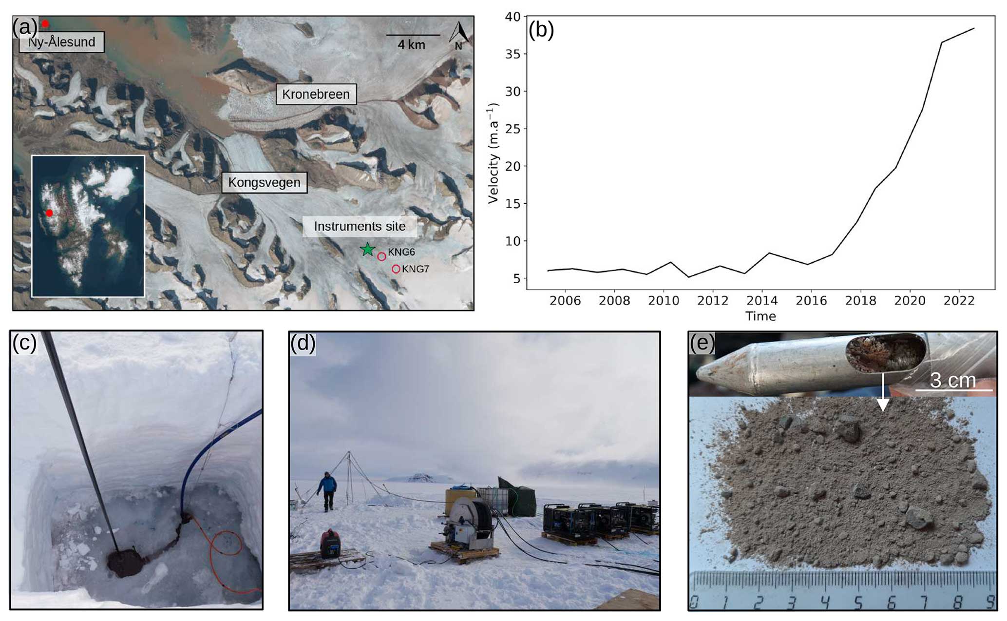
Figure 1 Study site and field methods. (a) Location of Kongsvegen in Svalbard. The green star indicates the instrument site where data were collected, and the red circles indicate the position of the GNSS KNG6 and KNG7 (credits: NPI/Copernicus Sentinel data). (b) Annual surface velocity near the equilibrium line of Kongsvegen glacier from 2005 to 2022, with an acceleration around 2014 witnessing that this glacier is closer to a surge event. (c) Main borehole with the smaller secondary borehole where the return pump is installed. (d) Drilling installation. (e) Sediment sample recovered with a sediment sampling tool at the bottom of the borehole.

3 Methods

3.1 Borehole

On 25 April 2021, we drilled a borehole near the long-term equilibrium line (78°18^′ N, 17°13^′ E; Fig. 1a) of Kongsvegen and placed instruments along the borehole and at its base. The borehole was drilled using a hot-water drilling system, consisting of three high-pressure hot-water machines (Kärcher HDS1000D), a $\mathrm{1}/\mathrm{2}$ in. diameter high-pressure hose, a 2 m drill stem with a 2.3 mm diameter nozzle, a pulley, a tripod, and water tanks (three 1000 L IBC tanks; Fig. 1d). Since the glacier was in winter conditions and liquid water was not available, the water flowing out of the borehole was captured in an auxiliary hole for recycling (Fig. 1c). During drilling, the level of water in the borehole started to drop when the drilling reached a depth of 260 m, indicating a connection to an active part of the drainage system. A sediment sample collected at the bottom of the ∼ 350 m borehole provides evidence for the existence of a sediment layer at the glacier bed (Fig. 1e). The borehole location has been chosen based on the work of Scholzen et al. (2021) and Pramanik et al. (2020), who suggested the existence of a preferential drainage axis in close proximity to this site.

At the bottom of the borehole, we installed a ploughmeter, i.e., a 1.4 m long steel rod equipped with strain gauges, to monitor mechanical conditions of the subglacial till (e.g., Humphrey et al., 1993; Iverson et al., 1994; Fischer and Clarke, 1994; Porter et al., 1997; Fischer et al., 1998, 2001; Murray and Porter, 2001; Boulton et al., 2001). The tip of the instrument penetrates into the till, whereas its upper part remains in the borehole and is trapped in the ice. As the glacier moves across its bed, the ploughmeter tip is dragged through the sediment and the device bends, which is sensed by the strain gauges. Strain on the ploughmeter is measured using a Wheatstone bridge for each pair of strain gauges in two perpendicular axes (Hoffmann, 1974). The exact insertion depth of the device into the till is uncertain. However, based on previous experiences with identical devices, we estimate the penetration depth to be in between 10 and 40 cm, which is sufficient to ensure that all strain gauges are immersed in the subglacial till. Just above the upper end of the ploughmeter (which is about 1 m above the glacier bed), we installed a vibrating wire pressure sensor (Geokon 4500SH, <2 kPa accuracy and 0.5 kPa resolution) to monitor subglacial water pressure, p. Sensor readings and data recording are performed using a Campbell Scientific CR1000X data logger, recording data at 1 min intervals. Ploughmeter measurements are converted to force experienced by the instrument while being dragged through the sediment, F. To do the conversion, we performed a calibration in the laboratory before the field deployment: masses of 10 and 50 kg (∼100 and ∼500 N) have been applied to the free end of the horizontally fixed ploughmeter in eight orientations (0 to 315° every 45°). After applying the calibration componentwise, we derive F from the x and y components using Pythagoras' theorem.

3.2 Near-surface instrumentation

At ∼ 100 m from the borehole, we installed a three-component geophone (DiGOS, 4.5 Hz) ∼ 1.5 m into the ice to ensure good coupling with the ice and to prevent meltout during summer. A DiGOS DATA-CUBE, which comprises a digitizer and a data logger, controlled the sampling rate (100 Hz) and recorded the signals. In this study, we analyze seismicity in the 3–10 Hz frequency band as a proxy for hydraulic conditions (Bartholomaus et al., 2015; Gimbert et al., 2016; Nanni et al., 2020; Lindner et al., 2020; Labedz et al., 2022). In addition, we used data from two surface stations (KNG6 and KNG7) that recorded positions using Global Navigation Satellite System (GNSS), from which we derived surface velocities. The stations are located at distances of 740 ± 10 m (KNG6; 78.78067° N, 13.15153° E) and 3100 ± 10 m (KNG7; 78.76770° N, 13.23962° E) upstream of the drill site. Data are continuously recorded at 5 s intervals between 1 April and 1 September, when solar panels help conserve battery capacity, but only for 1 h per day during the rest of the year. Gaps occurred in the time series when low battery voltage caused the data logger to fail. The GNSS data are processed assuming that the rover station is static for 1 h. Then the velocities are averaged daily to reduce the velocity uncertainties caused by the relatively low speed of the glacier. The Norwegian Mapping Authority's permanent network base station in Ny-Ålesund is used as a reference (baseline of ∼ 30 km). The two velocity records are merged; i.e., we consider the velocity derived from KNG6 when available and the one from KNG7 for the rest of the period (the original records for KNG6 and KNG7 can be seen in Appendix C). We apply a 1-week moving median for KNG7 velocity to smooth the record, especially during the winter period when the velocities are low. For the long-term averaged velocity from 2005 to 2022 (Fig. 1b), annual (April to April) glacier surface velocity was derived from annual GNSS surveys of mass balance stakes (Nuth et al., 2012).

3.3 Surface runoff and meteorological conditions

The surface runoff is modeled using the CryoGrid community model (Westermann et al., 2023). This model couples a surface energy balance model and a multi-layer snowpack model enabling the simulation of glacier mass balance and freshwater runoff (Schmidt et al., 2023). The model is forced by 3-hourly fields of near-surface conditions from the Copernicus Arctic Regional Reanalysis (CARRA; Schyberg et al., 2020; Yang et al., 2021) for 2021 and single-member forecasts by AROME-Arctic (Müller et al., 2017) for 2022. Differences in model results due to different forcing datasets are small in our study area (i.e., <2 % of the total runoff; Schmidt et al., 2023). Meteorological forcing includes 2 m air temperature and precipitation among other variables. The CryoGrid community model calculates the surface energy balance to simulate the mass balance components as well as the buildup and decay of seasonal snow. The available surface water in a grid cell is either retained in snow or firn or runs off under the influence of gravity. The retention is governed by the hydraulic conductivity of the snow, parameterized based on snow grain size, density, and effective water saturation. Depending on temperature conditions, retained water may refreeze, thereby releasing latent energy. Once the retention capacity of a layer is reached, excess water may run off with a timescale depending on surface slope. Schmidt et al. (2023) estimated a standard error of runoff of 0.12 m w.e. a⁻¹. The surface runoff is modeled on a 2.5 by 2.5 km grid. We determine the surface runoff routed through our study area by summing all surface runoff generated upstream from our study site within the glacierized catchment of Kongsvegen's glacier (Scholzen et al., 2021). Since our analysis considers relative changes, only the timing but not the absolute magnitude of the runoff is of interest. A complete description of the workflow is given by Schmidt et al. (2023). Using simulated surface runoff to represent local discharge through a given cross-section implicitly assumes the transfer of water between the surface and the base within a short time. The suitability of this hypothesis is reinforced by in situ observations from other Svalbard glaciers similar to Kongsvegen (Benn et al., 2009; Gulley, 2009; Bælum and Benn, 2011; Irvine-Fynn et al., 2011), and by the good agreement between daily values of simulated runoff, and measured proglacial discharge at the catchment scale (Schmidt et al., 2023). Therefore, we consider relative variations in surface runoff to represent those of subglacial discharge, even though large uncertainties on the magnitude of the subglacial discharge remain.

3.4 Derived subglacial variables

3.4.1 Seismic power, hydraulic radius, and hydraulic gradient

We calculate the seismic power, P, from the vertical component of the ground velocity using Welch's method over a 2 s time window with 50 % overlap (Welch, 1967; Beyreuther et al., 2010) within the frequency band 3 to 7 Hz. Our choice of this frequency band is based on the dominance of turbulent-water flow-induced seismicity in this frequency band (Gimbert et al., 2016; Nanni et al., 2020), as opposed to bedload transport that generates seismicity at higher frequencies (Gimbert et al., 2016). This turbulent-water flow-induced seismicity has been observed on different glacial settings (e.g., Bartholomaus et al., 2015; Preiswerk and Walter, 2018; Lindner et al., 2020; Nanni et al., 2021; Labedz et al., 2022; Clyne et al., 2023). Variations in this frequency band are related to changes in hydraulic radius, R, i.e., the ratio of the cross-sectional area of a channelized flow to its wetted perimeter, and in hydraulic gradient, S, i.e., the water pressure gradient in the along flow direction. For open channel flow, i.e., flow with a free surface, as opposed to pressurized flow, where the channel cross-section is filled with water in all directions, R scales with flow depth and S with slope along the flow direction. For glaciers, Gimbert et al. (2016) expressed P as a function of R and S. The relative changes of these variables are derived from relative changes in P and Q:

$$\begin{array}{}\text{(1)}& {\displaystyle \frac{S}{S_{\mathrm{ref}}}}={\left({\displaystyle \frac{P}{P_{\mathrm{ref}}}}\right)}^{\mathrm{24}/\mathrm{41}}{\left({\displaystyle \frac{Q}{Q_{\mathrm{ref}}}}\right)}^{-\mathrm{30}/\mathrm{41}}\text{(2)}& {\displaystyle \frac{R}{R_{\mathrm{ref}}}}={\left({\displaystyle \frac{P}{P_{\mathrm{ref}}}}\right)}^{-\mathrm{9}/\mathrm{82}}{\left({\displaystyle \frac{Q}{Q_{\mathrm{ref}}}}\right)}^{-\mathrm{21}/\mathrm{41}},\end{array}$$

where the subscript ref represents a reference state that must be defined over the same period for Q and P, but not necessarily for R and S. In our case, the reference state was taken on 24 June 2021 (Q_ref=0.08 m³ s⁻¹ and P_ref=180.59 dB), which corresponds to the pre-melt season 2021 value against which we want to evaluate relative changes happening during the melt season. The method is described in detail by Gimbert et al. (2016). Here, we neglect changes in conduit shape, degree of fullness, and number as they have limited impact on the derivation of R and S (Gimbert et al., 2016; Nanni et al., 2020). This approach allows one to estimate the evolution of R and S of the dominating drainage system over an area of ∼ 1 km² around the seismic station (Gimbert et al., 2016; Nanni et al., 2020; Lindner et al., 2020; Nanni et al., 2021; Labedz et al., 2022). To simplify notation, we hereafter refer to $R/R_{\mathrm{ref}}$ and $S/S_{\mathrm{ref}}$ as R and S respectively.

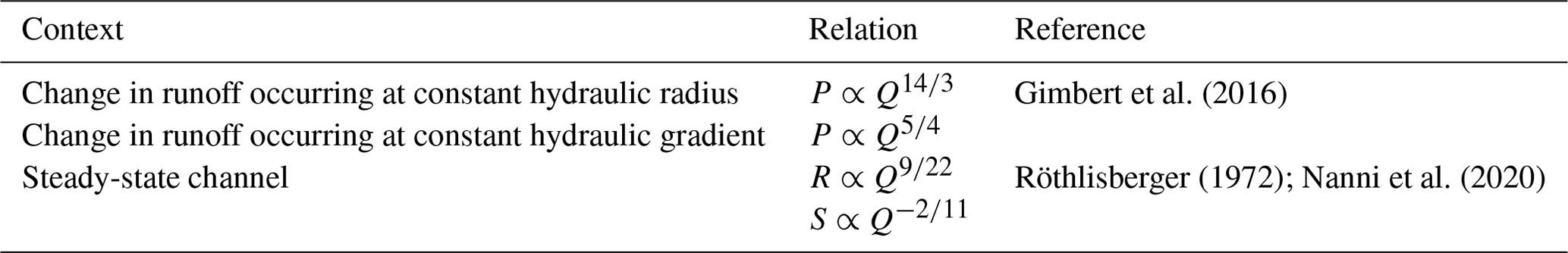
To discuss the state of the subglacial drainage system during the period of our records, we evaluate our results against scaling relationships linking P with Q (Gimbert et al., 2016) and R–S with Q (Röthlisberger, 1972; Nanni et al., 2020). The scaling relationship proposed by Gimbert et al. (2016) defines cases where steady-state channels incised in the ice adapt to changes in Q by only adjusting R (constant S) or the opposite case (constant R). Nanni et al. (2020) adapted Röthlisberger's (1972) theory to derive scaling relationships between R and Q, as well as S and Q, both for a steady-state channel evolution incised in the ice and for a channel of static cross-sectional area evolving as a rigid pipe (Table 1).

Gimbert et al. (2016)Röthlisberger (1972); Nanni et al. (2020)

Table 1 Scaling relationships between P and Q, S and Q, and R and Q, for special cases, derived by Gimbert et al. (2016) and Nanni et al. (2020) from the Röthlisberger (1972) theory to assess variations in channelized drainage conditions.

3.5 Processing of time series, catalog of events, and classification

To characterize subglacial conditions, we analyze the responses of the measured variables (force, F, and water pressure, p) and derived variables (turbulent-water-flow-induced seismic power, P, the hydraulic radius, R and the hydraulic gradient S) to the runoff, Q. Here we use the term “phase” to characterize the time relationship between one of the subglacial variables and the runoff. These phase relationships are analyzed at three different, glaciologically relevant timescales: seasonal, multi-day, and diurnal. To extract the corresponding components at these three timescales, we filtered the time series using a low-pass filter with a cutoff at 20 d, a band-pass filter between 4 and 8 d, and a band-pass filter between 6 and 36 h, respectively. We subdivide the multi-day and diurnal time series into individual events based on Q variations. We define an event by two subsequent minima of Q within the bandwidth investigated. We normalize both Q and the subglacial variables by their respective maxima and subdivide the time into 50 equidistant steps. The number of time steps was chosen empirically as the minimum number of data points that preserves the shape and characteristics of the event time series (see also Appendix B, Fig. B1). We synthesize the different responses of each subglacial variable, X, to changes in Q using a classification scheme (Fig. 2). Our workflow resembles that developed by Nanni et al. (2020) to understand subglacial hydrology on hard-bed glaciers and by Javed et al. (2021) to study storm-induced hydrological condition variations. The period of records is subdivided at a multi-day timescale into 12 events (melt season 2021; see Appendix D, Table D1) and 8 events (melt season 2022; see Appendix D, Table D2) and at a diurnal timescale into 96 events (melt season 2021; see Appendix D, Table D3) and 85 events (melt season 2022; see Appendix D, Table D4).

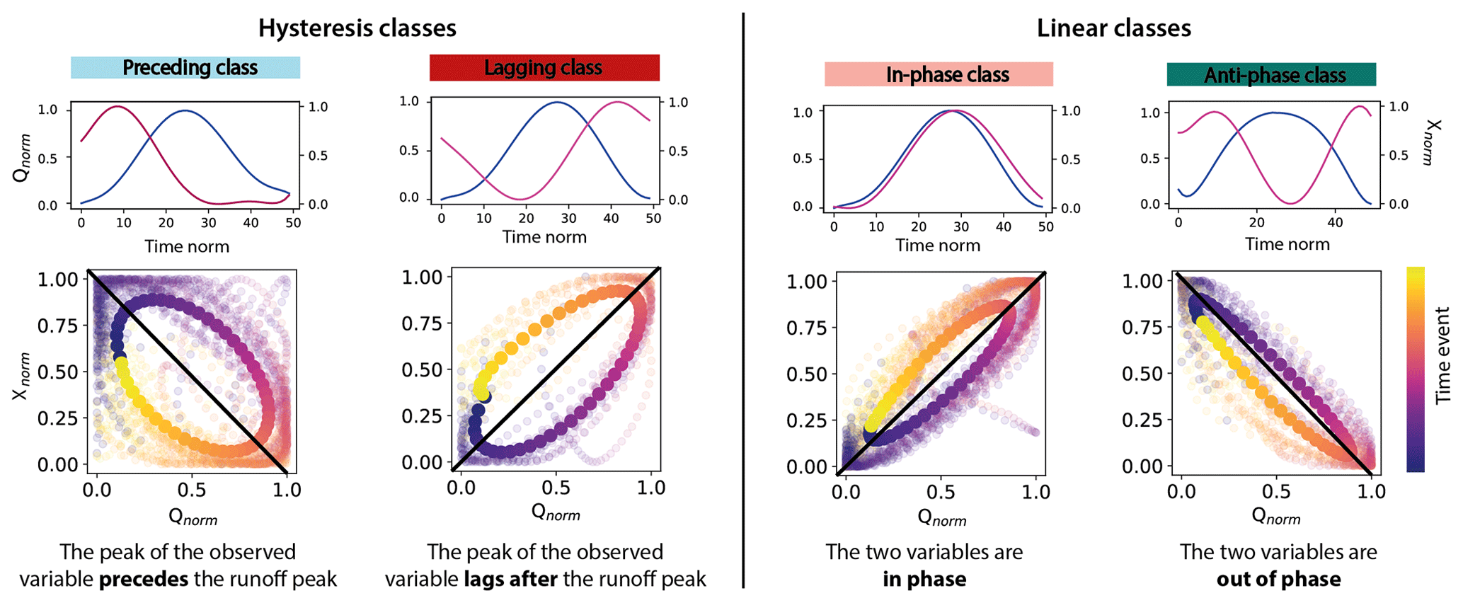
Figure 2 Phase relationship classification for events. Below each class, the plots in the first row correspond to a representative event for this class with runoff (Q_norm) plotted in blue and one subglacial variable (X_norm, with X being F, P, p, R or S) plotted in pink against time. The magnitude of the variables is normalized between 0 and 1, and the time is re-sampled into 50 time steps. The plots in the second row show the shape of the relationship between the two variables after classification. The solid color points refer to the mean behavior in this class; all individual events from the filtered time series are shown in shaded colors. The black line is the linear regression fitted to the scatter plot. Preceding class and lagging class correspond to clockwise or counterclockwise hysteresis (or time lag) between the runoff, Q, and the observed variable, while in-phase class and anti-phase class correspond to linear relationships. The color scale indicates chronology.

Our classification scheme is based upon the following metrics: the slope, m, of the linear regression between the subglacial variable X (with X being F, P, p, R, or S) and Q (black line, Fig. 2); the squared residuals, RSS, between the linear regression and the X_norm–Q_norm hysteresis loop; the direction of the hysteresis loop, θ. The spread of the data relative to the regression is quantified by the squared residuals (Appendix F, Fig. F1b):

$$\begin{array}{}\text{(3)}& \mathrm{RSS}=\sum _{i=\mathrm{1}}^n{r}_i^{\mathrm{2}},\end{array}$$

where r_i denotes the residuals of the regression.

The parameter θ expresses the asymmetry of the response to the forcing. Its sign determines whether the hysteresis is clockwise (positive) or counterclockwise (negative). We compute θ by comparing the mean of the subglacial variable during the rising limb of Q, ${\stackrel{\mathrm{‾}}{X}}_{Q_{\mathrm{rising}}}$, to its counterpart during decreasing Q, ${\stackrel{\mathrm{‾}}{X}}_{Q_{\mathrm{falling}}}$ (Appendix F, Fig. F1a):

$$\begin{array}{}\text{(4)}& \mathit{\theta }={\displaystyle \frac{{\stackrel{\mathrm{‾}}{X}}_{Q_{\mathrm{rising}}}-{\stackrel{\mathrm{‾}}{X}}_{Q_{\mathrm{falling}}}}{{\stackrel{\mathrm{‾}}{X}}_{Q_{\mathrm{falling}}}}}.\end{array}$$

The sign of θ indicates whether the signal precedes (θ>0) or lags (θ<0) Q.

Events are classified according to the phase relationship between Q and the subglacial variable. We distinguish four classes, representing the following cases (Fig. 2):

• Preceding class. The subglacial variable considered precedes Q, RSS >2 & θ>0.

• Lagging class. The subglacial variable considered lags behind Q, RSS >2 & θ<0.

• In-phase class. The subglacial variable considered and Q vary in phase, RSS ≤2 & m>0.

• Anti-phase class. The subglacial variable considered and Q vary in anti-phase, RSS ≤2 & m<0.

To discriminate between linear and hysteresis relations, we use a threshold of RSS =2, corresponding to a phase difference of about $\mathit{\pi }/\mathrm{10}$ for two sinusoidal variations. This threshold allows some deviation from a strictly linear behavior and accepts RSS ≤2 still representing linear behavior, thus taking into account uncertainties symptomatic for observations of natural systems. The choice of this threshold is motivated by visual observation of the clustering of phase relations (Fig. 2).

4 Results

4.1 Overview over the dataset

In Fig. 3, we show the meteorological conditions extracted from CARRA/AROME-Arctic, the velocity (u_s), the runoff (Q), the turbulent-water-flow-induced seismic power (P), the water pressure (p), and the force acting on the ploughmeter (F). We obtain time series covering two melt seasons (2021 and 2022; Fig. 3) and one winter period (Appendix A, Fig. A1). The meteorological conditions (Fig. 3a and b) control the timing and volume of Q resulting from meltwater production or rainfall (Fig. 3c and d). We note that the dataset covers two very different melt seasons. While the 2021 melt season is short (67 d from 1 July 2021 to 6 September 2021), marked by low temperature oscillating around 0 °C and continuous low runoff (lower than 20 m³ s⁻¹), the 2022 melt season is long (at least 83 d because we do not capture the end of this melt season, from 25 May 2022 to 16 August 2022), marked by high temperatures (up to 7 °C) accompanied by frequent and large excursions of runoff above 20 m³ s⁻¹.

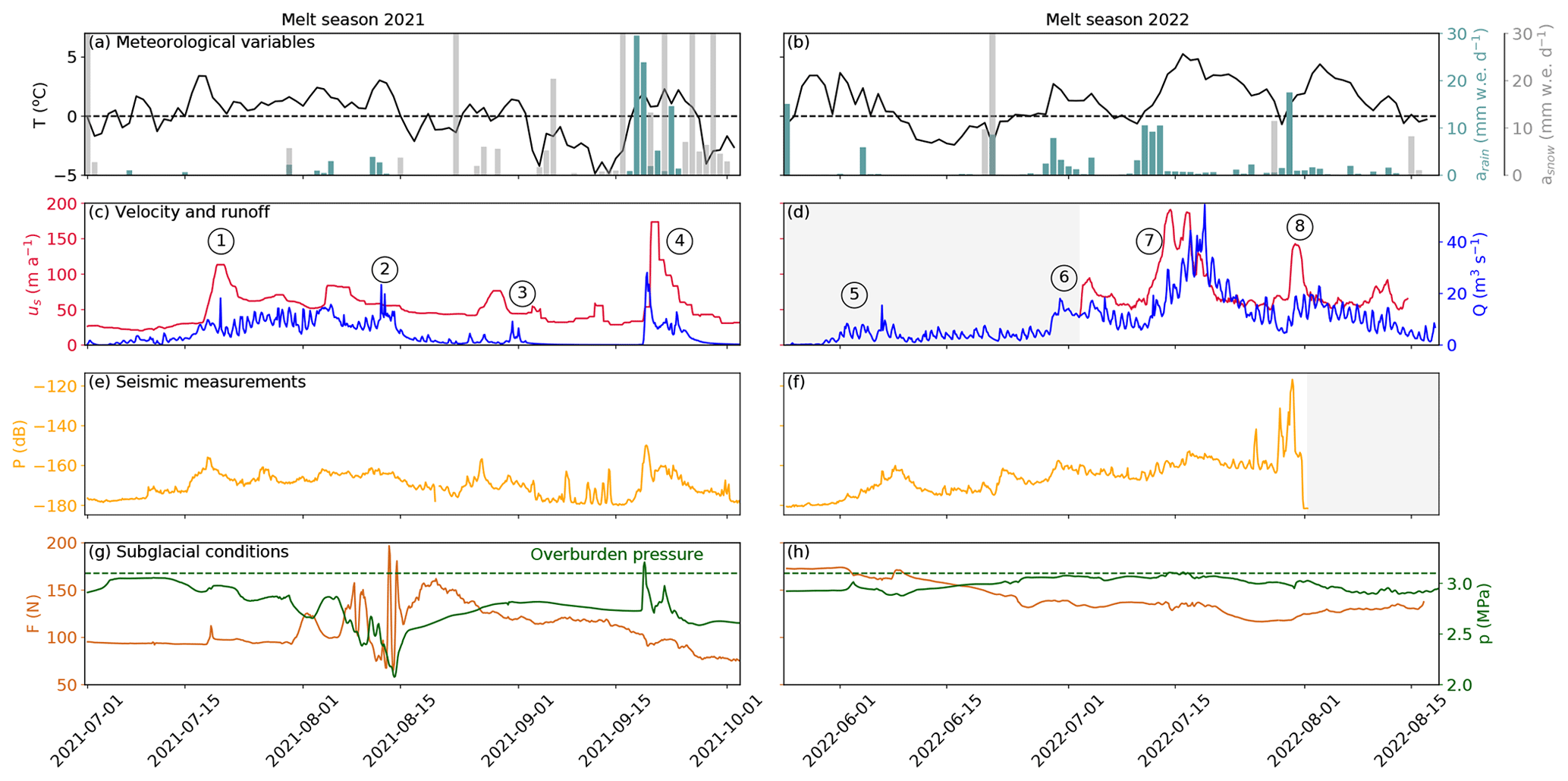
Figure 3 Time series of physical quantities measured during the melt seasons 2021 (a, c, e, g) and 2022 (b, d, f, h): (a–b) temperature (black line), snowfall rate (gray bars), and rainfall rate (light blue) from CARRA/AROME-Arctic (Schmidt et al., 2023). The three variables are extracted for the grid point closest to the borehole location. (c–d) Modeled runoff (blue) and measured glacier surface velocity (red). Circled numbers refer to episodes described in the main text. (e–f) Seismic power recorded at the surface of the glacier in the 3–10 Hz frequency band (yellow). (g–h) Borehole water pressure (green) and force acting on the ploughmeter (light maroon). Blue shaded areas represent the melt seasons. Gray shaded areas represent periods of missing data. The complete uninterrupted record spanning from spring 2021 to the end of summer 2022 is presented in Appendix A, Fig. A1.

In response to temperature and rainfall variations, Q displays variations on several timescales (Fig. 3c and d, blue line): (i) the seasonal timescale (>20 d) is marked by Q generally being limited to the melt season; (ii) the multi-day superimposed timescale (4–8 d) typically reflects weather variability (warm spells, e.g., Fig. 3c ②, or rainfall, e.g, Fig. 3c ④); (iii) and the pronounced diurnal variability of Q reflects the variability of surface energy balance.

The turbulent-water-flow-induced seismic power, P (Fig. 3e and f, yellow), follows the variations in Q throughout the recorded period, increasing at the beginning of the two melt seasons and decreasing towards their end. Such behavior has been previously observed in other settings and confirms the sensitivity of the selected frequency band to Q (Bartholomaus et al., 2015; Gimbert et al., 2016; Nanni et al., 2020; Lindner et al., 2020; Labedz et al., 2022). In contrast, variations in water pressure in the borehole, p, do not follow Q variations in a simple way (Fig. 3g and h, green). At the beginning of the 2021 melt season, p is high, close to the overburden pressure (3.2 MPa). As Q continues to increase, p decreases until it reaches its minimum values (∼ 2 MPa) after an abrupt increase in Q (②). p increases again during the winter to reach a value close to overburden pressure (2.9 MPa; Appendix A, Fig. A1d). In the second year of the record, p remains high and increases to the overburden pressure in mid-July 2022 before decreasing again to levels close to its winter value at the end of August 2022.

Similar to p, the force acting on the ploughmeter, F, shows different behaviors between the two melt seasons (Fig. 3g and h, dark red). During the melt season 2021, F remains fairly stable until August 2021, when it suddenly undergoes variations of large amplitude (∼ 150 N maximum amplitude) and high frequency. As the instrument site becomes snow-free around 15 August 2021 (Fig. 3a), F gradually decreases towards the end of the melt season until it reaches its minimum value in early October 2021 (∼ 70 N). At the end of September 2021 a major precipitation episode occurs (Fig. 3c ④). F does not react to this event. After this precipitation event, F gradually increases until it stabilizes at ∼ 170 N in January 2022. Note that this value is almost twice the value observed before the melt season 2021 (∼ 90 N).

The surface velocity of the glacier co-varies with Q-induced changes. We observe several glacier speed-up episodes: (i) early in the melt season 2021 when Q increased (Fig. 3c ①), (ii) during a large rainfall episode (Fig. 3c ④), (iii), and during sudden influx of meltwater during the 2022 melt season (Fig. 3d ⑥, ⑦, ⑧).

To interpret the responses of the subglacial drainage system and glacier dynamics to variations in runoff, Q, we analyze the data using a phase relationship analysis on seasonal (above 20 d; Sect. 4.2), multi-day (4–8 d; Sect. 4.3), and diurnal (6–36 h; Sect. 4.4) timescales.

4.2 Analysis of seasonal variations

To examine the phase relationship between the subglacial variables and Q at the seasonal scale, all time series are low-pass filtered with a cut-off frequency of 20 d. We first describe the results obtained for the melt season 2021 and then for the melt season 2022.

We observe four regimes during the melt season 2021. At the beginning of the melt season, the preferential drainage axis evolves predominantly by adjusting its capacity, R (constant hydraulic gradient, S; Fig. 4a, 1). As Q increases, we observe an adjustment of S at constant R (Fig. 4a, 2). When Q decreases in August 2021, the preferential drainage axis evolves by adjusting R (constant S; Fig. 4a, 3). At the end of the melt season 2021, we observe an adjustment of S (Fig. 4a, 4). Simultaneously, R–Q trajectory is parallel to the scaling relationship for channels evolving at steady state (Fig. 4b), and S–Q trajectory follows the steady-state relationship, though not always strictly parallel (Fig. 4c). At this time, the p–Q relationship is characterized by a clockwise hysteresis (Fig. 4d) indicating that the peak in p precedes the peak in Q. The linear relationship between F and p during the first half of the melt season indicates that the two subglacial variables are anti-correlated (Fig. 4e), and, at the end of the melt season, F–p trajectory shows a counterclockwise hysteresis, indicating that the peak in F lags after the peak in p (Fig. 4e).

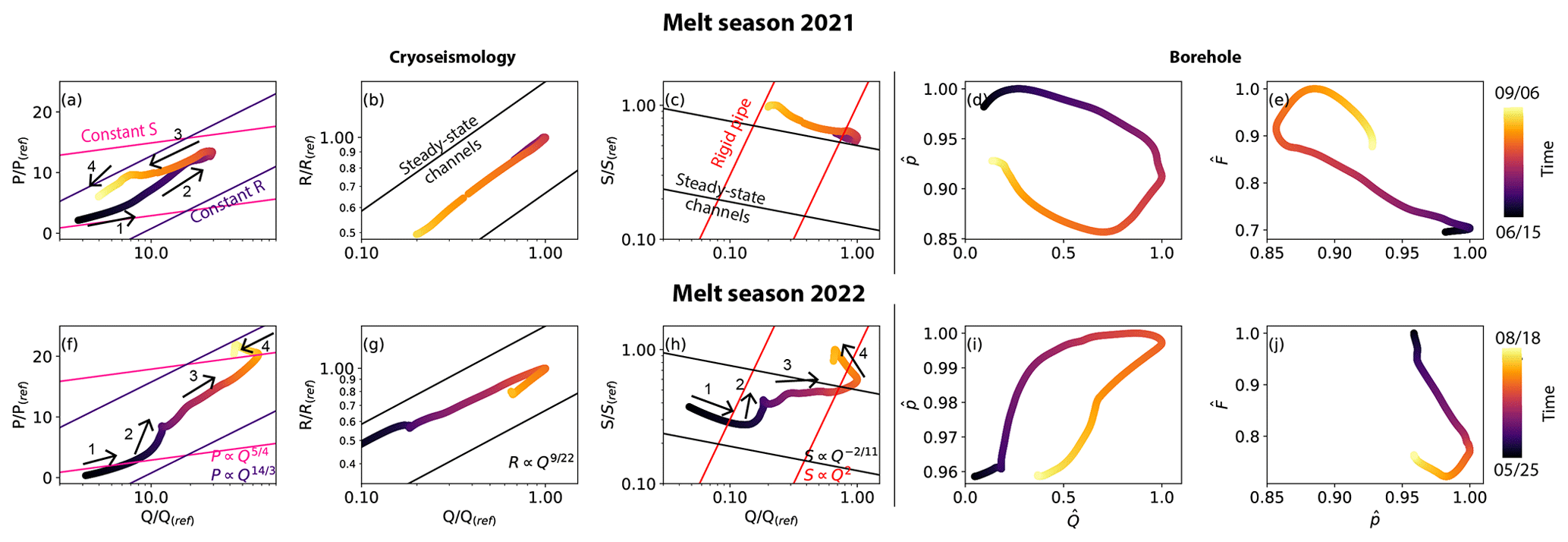
Figure 4 Relationships between two variables at the seasonal scale for the melt seasons 2021 and 2022. Colors are scaled to the number of days in each melt seasons. Panels (a) and (f) indicate relationships between scaled runoff ($Q/Q_{\mathrm{ref}}$) and scaled turbulent-water-flow-induced seismic power ($P/P_{\mathrm{ref}}$). The x axis is in logarithmic scale. The superimposed lines show the relations derived by Gimbert et al. (2016) for a constant hydraulic gradient (pink lines, $P\propto Q^{\mathrm{5}/\mathrm{4}}$) and for a constant hydraulic radius (purple curve, $P\propto Q^{\mathrm{14}/\mathrm{3}}$). Panels (b) and (g) indicate the relationship between scaled runoff ($Q/Q_{\mathrm{ref}}$) and scaled hydraulic radius ($R/R_{\mathrm{ref}}$). Both x and y axes are in logarithmic scale. Superimposed lines show the relations of steady-state preferential drainage axis evolution (Nanni et al., 2020; $R\propto Q^{\mathrm{9}/\mathrm{22}}$). Panels (c) and (h) indicate the relationship between scaled runoff ($Q/Q_{\mathrm{ref}}$) and scaled hydraulic gradient ($S/S_{\mathrm{ref}}$). Both x and y axes are in logarithmic scale. Superimposed lines show the relations of Nanni et al. (2020) for a preferential drainage axis at steady state (black lines; $S\propto Q^{-\mathrm{2}/\mathrm{11}}$) and for a preferential drainage axis evolving as a fixed cross-sectional area channel referred to as rigid pipe (red line; S∝Q²). Panels (d) and (i) indicate the relationship between normalized water pressure and normalized runoff. Panels (e) and (j) indicate the relation between normalized force and normalized water pressure. Arrows indicate the direction of time and numbers refer to different periods described in the main text. The numbers do not correspond to the same periods between each panels and are unrelated to the periods identified by the circled numbers in Fig. 3.

Similar to 2021, the melt season 2022 can be divided into four regimes, but these phases describe different behaviors. At the beginning of the melt season, the preferential drainage axis evolves predominantly by adjusting R (Fig. 4f, 1), as observed in 2021. Then, the preferential drainage axis briefly leaves this regime to follow an evolution that is not indicative of either constant R or constant S (Fig. 4f, 2). After this period, the preferential drainage axis follows a regime that is predominantly governed by adjustment of S (constant R) for the remaining increase in runoff (Fig. 4f, 3). The runoff decrease phase is not completely captured because the records do not extend to the end of the melt season 2022. For the period covered by data, we observe that the evolution of P is not indicative of either constant R or constant S (Fig. 4f, 4). We identify these four phases in the relationship of S and Q. During phases 1 and 3, the behavior is indicative of a preferential drainage axis evolving in equilibrium with Q (Fig. 4g and h, 1 and 3), while during phases 2 and 4, the behavior closely resembles that of a rigid pipe (Fig. 4g and h, 2 and 4). Over the whole melt season and as opposed to the melt season 2021, p and Q evolve almost in parallel. At the beginning of the melt season, p and Q are positively related even though the relationship displays some clockwise hysteresis (Fig. 4i). As for the melt season 2021, F and p are anti-correlated during the melt season 2022 (Fig. 4j).

4.3 Analysis at multi-day scale

To understand the relationships on the timescales of weather variations, we filtered the time series with a band-pass filter, removing the variations with periods below 4 d and above 8 d. Then, we applied our phase relationship classification scheme to each event (Fig. 5). We investigate the phase relationships between the subglacial variables (the force, F, the water pressure, p, the hydraulic radius, R, the hydraulic gradient, S) and the runoff, Q, for each event during the melt seasons in 2021 (11 events) and 2022 (8 events; see Sect. 3.5). Similar phase relationships are observed during both melt seasons between (i) R and Q and (ii) S and Q. During both melt seasons, R evolves in phase with Q (in-phase class; Fig. 5a and c). S evolves in phase with Q only at the beginning of the melt season 2021 (in-phase class; Fig. 5a). We cannot compare the relationship between S and Q at the beginning of the melt season 2022 due to inconsistencies between the filtered and raw data, necessitating their exclusion from the analysis (Appendix G, Fig. G1). For the remaining part of the season, the behavior of S in response to Q is very similar in 2021 and 2022. During the first half of both melt seasons, S is first lagging after Q (lagging class; Fig. 5a and c). During Q important events of August 2021 (Fig. 5b ②) and July 2022 (Fig. 5d ⑦), S precedes Q changes (preceding class; Fig. 5a and b). In contrast to the phase relationships of R and S to Q, F does not show the same time evolution across both melt seasons. The F–Q phase relationship is sensitive to glacier acceleration. During high-velocity episodes (Fig. 5b and d ①, ④, ⑦), F systematically lags behind Q (lagging class; Fig. 5a and c). Conversely, when velocity is low and stable during the melt season 2021 (Fig. 5b and d, from ① to ③), F is anti-correlated with Q (Fig. 5a and c). We do not have GNSS data in 2022 at this period to compare with the observations in 2021. Between the melt season 2021 and 2022, the p–Q relationship is contrasted. On the one hand, the p–Q phase relationship cannot be easily linked to specific Q regimes or speed-up episodes and shows various responses across the melt season 2021 (lagging class, in-phase class, and anti-phase class; Fig. 5a and c). On the other hand, p always precedes Q during the melt season 2022 (preceding class; Fig. 5c).

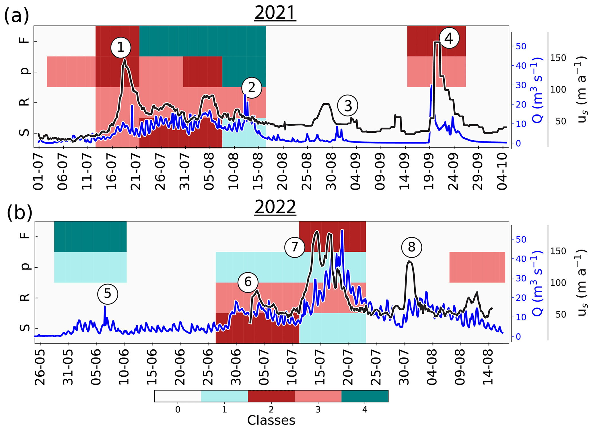
Figure 5 Phase relationships between the subglacial variables (S, R, p, and F) and runoff (Q) at a multi-day timescale. Panel (a) shows the classification for the melt season 2021 and panel (b) the melt season 2022. Gray fields refer to periods when data are missing, and the vertical gray lines delineate the events. Preceding class and lagging class correspond to clockwise or counterclockwise hysteresis between the runoff and the observed variable, while classes in-phase class and anti-phase class correspond to linear relationships. In addition, the time series of velocity (gray line) and runoff (blue line) are super-imposed on each panel. Circled numbers refers to episodes described in Sect. 4.1.

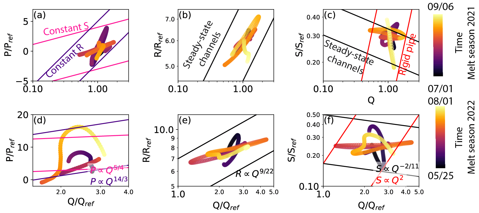
Figure 6 Relationship between the subglacial variables ($P/P_{\mathrm{ref}}$, $R/R_{\mathrm{ref}}$, $S/S_{\mathrm{ref}}$) and runoff ($Q/Q_{\mathrm{ref}}$) during the two melt seasons at a multi-day timescale. The color scale indicates the timing during both melt seasons and is scaled according to the length of each season. Panels (a) and (d) indicate the relationship between scaled runoff ($Q/Q_{\mathrm{ref}}$) and scaled turbulent-water-flow-induced seismic power ($P/P_{\mathrm{ref}}$). The x axis is in logarithmic scale. The superimposed lines show the relations derived by Gimbert et al. (2016) for a constant hydraulic gradient (pink lines, $P\propto Q^{\mathrm{5}/\mathrm{4}}$) and for a constant hydraulic radius (purple curve, $P\propto Q^{\mathrm{14}/\mathrm{3}}$). Panels (b) and (e) indicate the relationship between scaled runoff ($Q/Q_{\mathrm{ref}}$) and scaled hydraulic radius ($R/R_{\mathrm{ref}}$). Both x and y axes are in logarithmic scale. Superimposed lines show the relations for a steady-state channel evolution (Nanni et al., 2020; $R\propto Q^{\mathrm{9}/\mathrm{22}}$). Panels (c) and (f) indicate the relationship between scaled runoff ($Q/Q_{\mathrm{ref}}$) and scaled hydraulic gradient ($S/S_{\mathrm{ref}}$). x and y axes are in logarithmic scale. Superimposed lines show the relations of Nanni et al. (2020) for a channel evolution (black lines; $S\propto Q^{-\mathrm{2}/\mathrm{11}}$) and for a channel evolving as a rigid pipe of static cross-section (red line; S∝Q²).

Figure 6 shows the comparison between the multi-day scale observations of P, R, and S and the scaling relationships by Gimbert et al. (2016) and Nanni et al. (2020). At the beginning of the melt season 2021 (July 2021), the slope of the P–Q relationship exceeds those of the constant R or constant S scaling relationships. Then, the P–Q relationship indicates a preferential drainage axis evolving at a constant S in the middle of the melt season (August 2021; Fig. 6a). At the end of the melt season, P switches back to the behavior seen at the beginning of the melt season 2021 (Fig. 6a). In general, R evolves with Q similar to what is expected for a steady-state channel (Fig. 6b), whereas S shows a more complex behavior that is difficult to disentangle (Fig. 6c).

During the melt season 2022, the evolution of P is clearly dominated by neither a constant R nor S (Fig. 6d). In general, R increases with Q but at a slope that differs from the one expected for steady-state channels (Fig. 6e). As in 2021, the evolution of S exhibits complex behavior at this scale during the melt season 2022 (Fig. 6f).

4.4 Analysis of diurnal variations

Symptomatic for glacier meltwater runoff, Q exhibits strong diurnal variations. To examine the glacier response to changes in Q at a diurnal scale, we filtered the time series using a band-pass filter removing the variations with periods below 6 h and above 36 h (Fig. 7). In analyzing variations within this band, we aim primarily to capture the diurnal variation (around 24 h) and to take account of certain fluctuations around this period. The filtered time series are then subdivided into 95 events in 2021 and 84 events in 2022 (see Sect. 3.5), and we applied our phase relationship classification scheme.

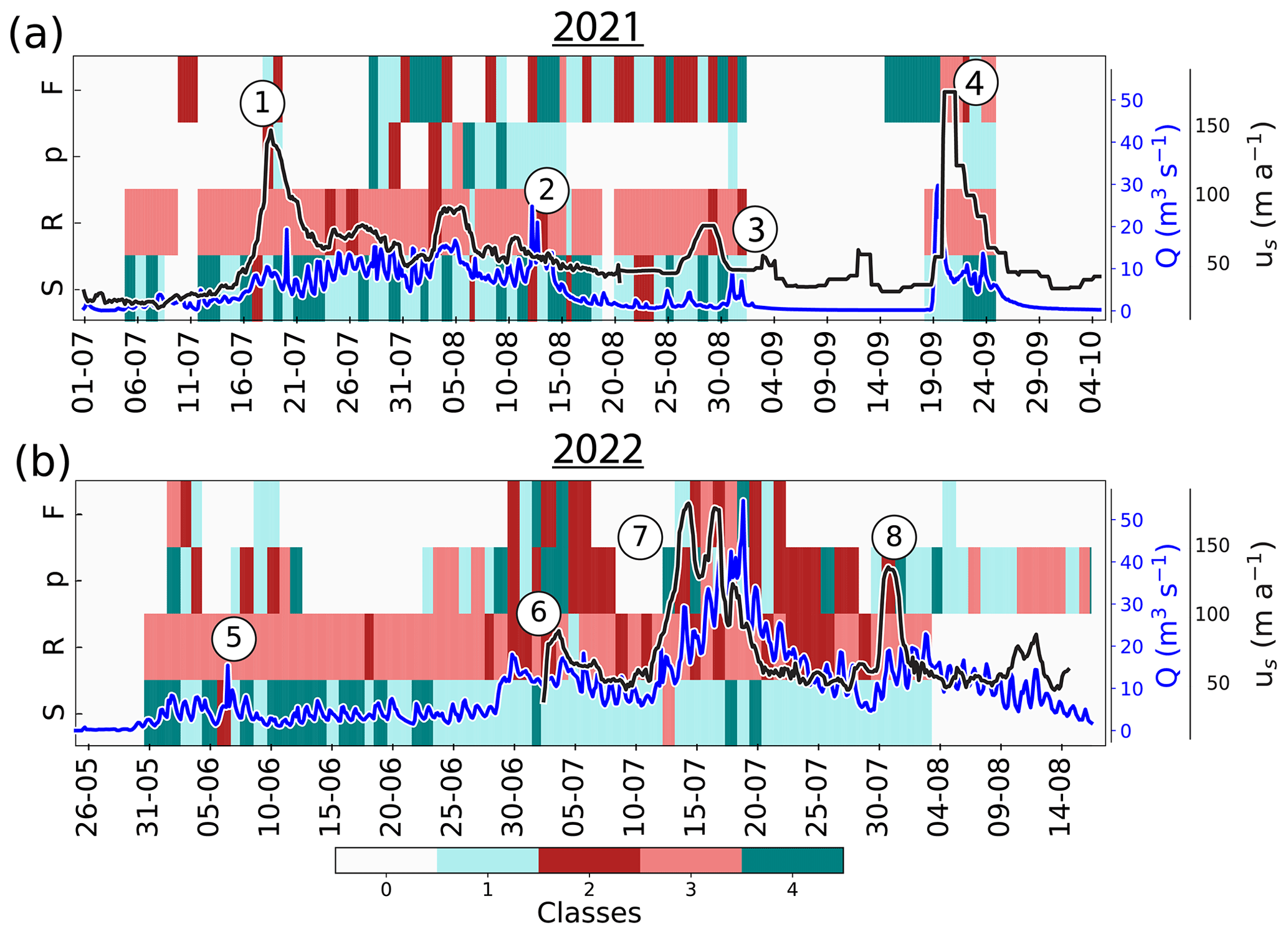
Figure 7 Phase relationships between the subglacial variables (S, R, p, and F) and runoff (Q) at a diurnal timescale. (a) Classes from the phase relationship classification per event for the melt season 2021 and (b) for the melt season 2022. Gray fields refer to periods when data are missing, and the vertical gray line delineates the events. In addition, the time series of velocity (gray) and runoff (blue) are super-imposed on each panel. Circled numbers refer to episodes described in Sect. 4.1.

The phase relationships between the subglacial variables (the force, F, the water pressure, p, the hydraulic radius, R, the hydraulic gradient, S) and Q on a diurnal timescale are displayed in Fig. 7. We observe that R and S show consistent phase relationships with Q during the melt seasons 2021 and 2022, alternating between lagging class and preceding class, as well as preceding class and anti-phase class, respectively (Fig. 2). However, the p–Q and F–Q relationships vary across all classes without an easily identifiable pattern (Fig. 7a–c). Except for during short episodes, p and F do not display pronounced diurnal variations (Appendix H, Fig. H1). Therefore, we focus on the analysis of diurnal variations on the responses of P, R, and S.

During the 2021 melt season, we observe that R mostly varies in phase with Q (in-phase class; Fig. 7a). S is mostly anti-correlated with or precedes Q (preceding class or anti-phase class; Fig. 7a).

During the melt season 2022, we observe a shift from linear responses of R and S (in-phase class and anti-phase class; Fig. 7b) towards more hysteretic responses (preceding class and lagging class; Fig. 7b) when Q shows the first significant increase in June (Fig. 7b ⑥). Before this event, R varies with changes in Q (in-phase class; Fig. 7b), but after, R lags behind Q (lagging class; Fig. 7b). Similarly, S shifts regimes from being anti-correlated with Q before the event ⑥ (anti-phase class; Fig. 7b) to a regime where S precedes Q after this event (preceding class; Fig. 7b).

5 Discussion

5.1 Interpreting the evolution of subglacial conditions

In this study, we have analyzed variations in subglacial hydro-mechanical conditions, i.e., the response of subglacial variables to changes in runoff, and we interpret now the observed behavior in terms of subglacial drainage system evolution (Sect. 5.2) and till rheology (Sect. 5.3). We divided the relationships observed between different subglacial variables (the force, F, the water pressure, p, the hydraulic gradient, S, and the hydraulic radius, R) and runoff, Q, into four classes (Fig. 2). Here, we first consider the expected responses of R, S (Eqs. 1 and 2) and p to changes in Q for different typical stages of subglacial channel evolution. In addition, we discuss the expected responses of F for the Coulomb plastic rheology and discuss why the observed relationships may not differ from the current theory. Second, we apply this interpretation scheme to the observed behavior separately for each of the considered timescales, before we consolidate these interpretations into a coherent picture of subglacial conditions.

Due to the relatively low bed slope and the long distance between our borehole location and the glacier front, unpressurized drainage is unlikely to persist, and open flow paths are expected to close quickly (Nye, 1976). For a drainage axis with a fixed cross-sectional area (rigid pipe), an increase in runoff, Q, is expected to result in increasing water pressure, p, that translates to a positive, linear p–Q relationship (in-phase class; Fig. 2). In this situation, we expect a constant hydraulic radius (R), unaffected by variations in runoff (Q, not classified) and concomitant acceleration events. Since we always measure the water pressure (p) at the same location and the glacier terminus is fixed at sea level, for a spatially homogeneous drainage system, we expect that variations in hydraulic gradient (S) are closely related to those of water pressure (p). However, spatiotemporal complexity in the drainage system downstream of our borehole may lead to incoherent relations between local water pressure (p) and spatially integrated hydraulic gradient (S). According to Röthlisberger's theory for ice-walled channels, the channel cross-section is determined by the two counter-acting processes of (1) opening by melting due to dissipation of potential energy and (2) creep closure of the surrounding ice. In steady state, these two processes balance each other, and a large runoff is associated with a large channel, thus causing low hydraulic gradient (S) and water pressure (p) (Schoof, 2010; Werder et al., 2013). In this situation, the glacier velocity is expected to remain constant or decrease. We interpret a negative, linear relationship (anti-phase class; Fig. 2) between runoff (Q) and water pressure (p, and similar for S and Q), as indicative of steady-state drainage of a preferential drainage axis. In this configuration, the hydraulic radius (R) increases with runoff (Q) (in-phase class; Fig. 2). The evolution of the drainage system in response to runoff (Q) is typically transient between the two end-members described above, evolving as a rigid pipe on the one hand and a steady-state channel on the other hand. For transient evolution between these two end-members, we expect a hysteretic behavior in the phase relationships between subglacial variables and runoff (Q). Evolution towards steady state occurs with some time delay; if variations of runoff (Q) occur faster than this delay, the variations of hydraulic radius (R) lag the variations of runoff (Q), resulting in a counterclockwise hysteresis (lagging class; Fig. 2). For such a transient evolution, hydraulic radius (R) is smaller during the rising limb of runoff (Q) than during its decrease, resulting in a counterclockwise R–Q hysteresis (lagging class; Fig. 2). At the same time, the larger hydraulic radius (R) during the decrease of runoff (Q) requires a lower water pressure (p) to drive the flow, resulting in a clockwise hysteresis in the p–Q relationship (preceding class; Fig. 2). As stated above, we expect the hydraulic gradient (S) to vary similarly to water pressure (p).

We interpret the force (F) variations experienced by the ploughmeter assuming a Coulomb plastic flow law for till (Iverson et al., 1998). The till shear strength depends directly on the pore-water pressure, which we assume to co-vary with water pressure (p) at the bottom of the borehole (Iken and Bindschadler, 1986; Hooke et al., 1997; Zoet and Iverson, 2020; Gilbert et al., 2022). This behavior would result in a negative, linear relationship between force (F) and water pressure (p) (anti-phase class; Fig. 2). In that case, high water pressure would weaken the till, facilitating its deformation (e.g., Weertman, 1957; Lliboutry, 1968). However, more complex F–p relationships can occur, arising from the non-linearity of the water pressure–sliding speed relationship (Alley, 1989; Boulton and Hindmarsh, 1987) and from the degree of ice–till coupling (Iverson et al., 2007). water pressure (p) and force (F) can also be influenced by potential distal forcing, e.g., longitudinal stress transfer, complicating their interpretation. Additionally, as water pressure, p (and hydraulic gradient, S), depends both on runoff (Q) and the efficiency of the subglacial drainage system, F–Q relationships are difficult to interpret.

Our interpretation scheme described here lets us expect a limited number of options for the classification of phase relations between each subglacial variable and runoff (Q). For p–Q and S–Q, we expect behaviors according to preceding class, in-phase class or anti-phase class; we expect R–Q to display either lagging class or in-phase class behavior; F–p is expected to fall either in in-phase class or anti-phase class; direct F–Q relations are not easily interpretable. In practice, we observe that some events are classified outside the expected range (Figs. 5 and 7). The occurrence of such behavior may be attributed partly to artifacts introduced by the spectral filtering applied to the time series for the analysis. Although we manually checked the consistency between the unfiltered and filtered signals to remove the most apparent differences (see Sect. 3.5), some inconsistencies may remain. Small shifts in timing of peaks may be amplified by normalizing the event time axis and hence lead to misclassification of some events. In addition, the definition of the four classes is motivated by noticing that phase relations may be linearly positive or negative or exhibit some transitory stage (preceding or lagging).

5.2 Subglacial drainage system evolution

The two observed melt seasons considerably differ in terms of duration, variability, and melt rate (Fig. 3). Whereas in 2021, melting occurs over a relatively short period and yields low levels of water supply, the melt season 2022 lasts longer and is characterized by higher temperatures, leading to higher water supply rates. This difference provides the opportunity to study the evolution of the subglacial drainage system in response to very different forcing.

5.2.1 The melt season 2021: short duration and low melt rate

The melt season 2021 is short (67 d) and marked by runoff usually lower than 20 m³ s⁻¹ (Fig. 3a). Applying our interpretation scheme to the observed responses of the water pressure, p, the turbulent-water-flow-induced seismic power, P, the hydraulic radius, R, and the hydraulic gradient, S, yields a largely consistent picture of a subglacial drainage system that fully adapts to seasonal runoff variations. The p–Q relationship exhibits clockwise hysteresis, indicative of system capacity growing with runoff (Fig. 4d). R–Q variations are positively linearly related (Fig. 4b). The S–Q relationship covers only the declining phase of runoff (Q) and shows an increase of hydraulic gradient (S) during this decrease, consistent with the above interpretation (Fig. 4c). Although all records draw the picture of a system adjusting to runoff (Q) variations, there is a noteworthy difference in the interpretations of borehole measurements and those of cryoseismology records. While long-term variations of hydraulic radius (R) and hydraulic gradient (S) suggest that the system capacity reaches an equilibrium with runoff (Q), the variations of water pressure (p) indicate a transient evolution in response to changes in runoff (Q), indicative of system capacity growing with runoff. We explain this apparent disagreement by the different spatial scales of sensing of the different instruments: while the geophone records are likely dominated by seismicity generated by turbulent flow in the channelized system (Nanni et al., 2021), the pressure record is representative of the local conditions at the borehole location, which is more likely to sense the local distributed system (Rada and Schoof, 2018).

The theoretical timescale of channel adjustment is usually longer (several days to weeks) than typical variations in runoff (hours) (Röthlisberger, 1972). At short timescales, drainage pathways are thus either overwhelmed when runoff (Q) increases or partially filled when runoff (Q) decreases, which results in a response similar to that of a rigid pipe (fixed cross-sectional area channel) rather than that of a steady-state channel (variable cross-section determined by the balance between melt opening and creep-closure to cope with runoff variations). We therefore expect a predominance of in-phase class for the p–Q and S–Q relationships over multi-day and diurnal timescales (Figs. 5a and 7a). The multi-day classifications of p–Q and S–Q relationships mainly support this view by displaying lagging class and in-phase class behaviors (Fig. 5a); however, on diurnal timescales (Fig. 7a), the picture is less clear likely due to changes in roughness (e.g., roughness of the ice walls and/or of the underlying bed) in the subglacial drainage system (Nanni et al., 2020).

We observe that the melt-induced runoff increase at the beginning of the melt season and a major rainfall event at its end (Fig. 3, ① and ④) leave a clear impact on water pressure (p) at the multi-day timescale (Figs. 3d, 5a), which coincides with a considerable glacier acceleration. During these events, the p–Q relationship indicates that the drainage system evolves transiently (lagging class and in-phase class; Fig. 5a). We suggest that at the beginning of the melt season, the drainage system is not yet developed leading to an immediate increase in water pressure (p). At the end of the melt season, runoff (Q) was at low levels for a period of about 10 d (Fig. 3d), and presumably, the capacity of the drainage system had decreased, when it suddenly became overwhelmed by the arrival of new water volumes. This results in a sharp increase in water pressure (p), provoking a short-term acceleration of the glacier. Similar late-season events have also been reported in other studies (Andrews et al., 2014; Rada and Schoof, 2018; Nanni et al., 2023). Even though water pressure (p) supports the interpretation of the velocity data in this context, the p–Q relationship displays similar patterns throughout the 2021 melt season, which do not lead to acceleration events.

5.2.2 The melt season 2022: long duration and high melt rate

In contrast to the melt season 2021, the melt season 2022 is long (at least 83 d since our records end before the melt season ceases) and contains frequent and large excursions of runoff (Q) above 20 m³ s⁻¹ (Fig. 3a) leading to a different evolution of the subglacial drainage system. the R–Q relationship is linearly positive, indicating that the drainage system capacity evolves at equilibrium with runoff (Q) (Fig. 4g). The S–Q relationship follows a trajectory that first is typical of a steady-state channel (Fig. 4h, 1) before shifting to a positive slope similar to that expected for a rigid pipe (Fig. 4h, 2, 3, and 4). Such behavior is typical for a system that is continuously overwhelmed since the subglacial preferential drainage axes cannot adapt fast enough to increasing runoff (Q). This period (Fig. 4h, 2, 3, and 4) coincides with a noticeable glacier acceleration event aligning with a subglacial drainage system out of equilibrium. This acceleration indicates a direct link between glacier velocity and the state of the subglacial drainage system as measured locally and possibly in isolated bed regions (Figs. 3h ⑦, 4i). The P–Q relationship in 2022 shows similar behavior to that in 2021, if we take into account that the 2022 record does not cover the decrease of runoff (Q) (Fig. 4f). The view of a continuously overwhelmed drainage system is further supported by the generally positive slope of the p–Q relationship that has a considerably smaller clockwise hysteresis compared to the preceding year (Fig. 4i).

Over shorter timescales, the classifications of R–Q and S–Q exhibit similar behavior as in 2021 (Figs. 5b and 7b), indicative of system adjustment also on multi-day and diurnal times. However, the lagging class behavior of S–Q at the beginning of the melt season visible in Fig. 5b remains difficult to explain. On a diurnal timescale, the dominance of anti-phase class in the S–Q relationship before July 2022 suggests that preferential drainage axis evolution is in equilibrium with runoff (Q; Fig. 7b). We observe a switch in the data to mainly preceding class behavior, which in turn is indicative of a transient evolution, typical for a drainage system that cannot adapt fast enough to the runoff variations. The R–Q relationship exhibits a similar switch (from in-phase class to class II 7b) with implications consistent with the interpretation above. The preceding class behavior of p–Q on multi-day scales further supports the transient evolution of the subglacial drainage system at this scale. However, as opposed to the acceleration events during the melt season 2021 (Fig. 3h ① and ④), there is no straightforward explanation between the p–Q relationship and the acceleration event observed during the melt season 2022 (Fig. 3h ⑦). We suggest that, here, the glacier acceleration is controlled by processes not happening locally and thus not recorded locally by the water pressure sensor. The diurnal scale (Fig. 7b) reveals that there are more diurnal variations in water pressure (p) during the melt season 2022, compared to 2021 (more events are classified). However, the diurnal analysis renders a blurry picture since all classes occur and no clear pattern can be depicted (Fig. 3d).

5.2.3 Ambiguous interpretation from borehole and cryoseismic records

In the previous section, we interpreted the multi-variable record in terms of drainage system evolution in response to runoff (summarized in Fig. 9). We note that, sometimes, interpretations derived from different records are ambiguous. For instance, during the melt season 2021 on a seasonal scale, the relationships between the cryoseismic record (P) with Q, as well as derived variables (R and S) with Q, yield a picture of a subglacial drainage system in equilibrium with runoff (Q). In contrast, the p–Q relationship based on the borehole record is symptomatic of a transient evolution where geometric adjustments lag variations in runoff (Q). Another example of the ambiguity is found in the analysis of diurnal variations in 2022 (Fig. 7b) where the cryoseismic records indicate a switch from an equilibrium to a transient evolution coinciding with a major increase in runoff (Q, Fig. 7d ⑥). The corresponding classification of the p–Q relationship is less conclusive about a similar switch and exhibits variations over all classes with no clearly recognizable pattern. In this section, we discuss potential sources for these inconsistencies and how these may be resolved.

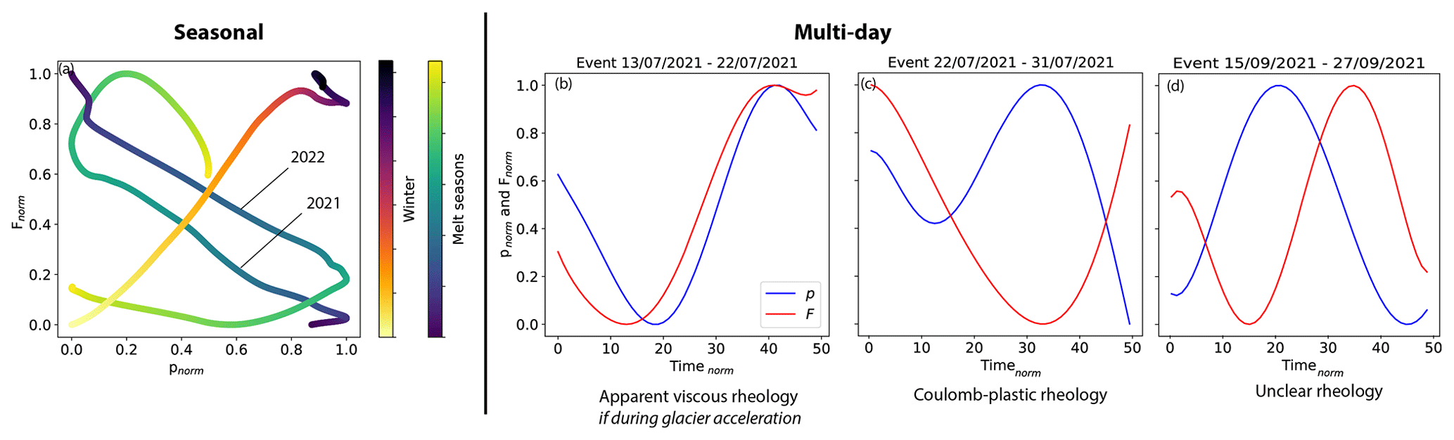
Figure 8 Comparison between the variations of water pressure p and ploughmeter force F (a) at the seasonal and (b)–(d) multi-day timescales. (a) Relationship between p and F at the seasonal timescale. F and p are normalized (min–max normalization) to be comparable. Blue–yellow and yellow–purple color scales indicate time during melt seasons and winter, respectively. (b) Evolutions of F (red) and p (blue) for an event indicative of apparent viscous behavior (assuming that p is positively related to basal motion). Similar behavior has been observed also during other periods (e.g., from 13 to 22 July 2021, and 8 to 17 August 2021). The time of the event is normalized over 50 time steps. (c) Evolutions of F (red) and p (blue) for an event indicative of Coulomb plastic behavior. Similar behavior has been observed also during other periods (e.g., from 22 to 31 July 2021, from 7 July 2021 to 8 August 2021, and from 11 to 23 July 2022). The time of the event is normalized over 50 time steps. (d) Evolutions of F (red) and p (blue) that remain unclear as the interpretation scheme does not provide a clear indication of till rheology. Similar behavior has been observed also during other periods (e.g., from 15 to 27 September 2021, and from 28 May 2022 to 6 June 2022). The time of the event is normalized over 50 time steps. Simultaneous multi-day variations of F and p can be assessed only for five and two events during the melt seasons 2021 and 2022, respectively. All panels show normalized variations of F and p.

In our case, P integrates the seismicity in the 3–10 Hz frequency band in which seismic wavelengths are of the order of 150–500 m (for typical surface wave velocity of the order of 1500 m s⁻¹; Köhler et al., 2012; Gimbert et al., 2021b). Accordingly, the cryoseismologically derived variables P, R, and S are sensitive to an area of ∼ 1 km² around the geophone location. In addition, since the seismicity in this frequency range is mainly generated by turbulent water flow, we expect that the observed signal is mainly indicative of large channels (Nanni et al., 2021). In contrast, water pressure (p) is measured at the bottom of the borehole, estimated to be ∼ 20 cm in diameter at the base of the glacier. Depending on the hydraulic connection of the borehole and the ice–till coupling, water pressure (p) may be representative of about 1 m² in the case of hydraulic isolation or for an area several orders of magnitude larger in the case of a direct connection to a preferential drainage axis (Murray and Clarke, 1995; Mair et al., 2001, 2003). As a consequence, interpreting the cause of glacier acceleration through cryoseismology or local basal water pressure might not be suitable. On the one hand, cryoseismology is sensitive to the most efficient part of the subglacial drainage system that is often not the primary controller of glacier velocity. On the other hand, glacier velocity results from basal conditions over a larger area (scale of ice thickness) than what is locally sampled by the measured water pressure (p).

In addition, the hot-water drilling operation might have disturbed the subglacial environment (excavation of fines, volume of water pushed to the bed), influencing the water pressure observation. However, the volume of water injected through hydraulic connection of the borehole to the bed is limited (∼ 0.5 m³ for the observed 30 m drop of the water column at the connection), and the borehole was drilled at beginning of May 2021. In the absence of surface melting before late June 2021, it seems unlikely that a potential initial connection could be maintained. Geometrically controlled patterns of channelization on a hard bed may be persistent, but a soft sediment bed provides less geometrical control on the spatial patterns, and year-to-year variability of channel location within a few meters seems plausible. In addition, several studies report that water pressure records displayed regime changes and suggest that these may reflect reorganization of the drainage system (Gordon et al., 1998; Kavanaugh and Clarke, 2000; Schuler et al., 2002; Andrews et al., 2014; Rada and Schoof, 2018). Resuming the idea of a spatially heterogeneous and discontinuous drainage system aids in resolving the apparent discrepancies derived from the different records: if the active drainage system within 1 km² around our instrument site is in equilibrium with runoff (Q), the seismological record would reveal this effect, whereas the borehole record may reveal a different interpretation if the borehole itself is located in a less well connected or even isolated part of the glacier bed. The apparent discrepancy derived from different records therefore supports the comprehension of the drainage system as a discontinuous, spatially heterogeneous sheet. Although the minor diurnal variability and high values of water pressure (p) during the melt season 2022 may be interpreted as symptomatic for hydraulic isolation (Rada and Schoof, 2018; Rada Giacaman and Schoof, 2023), p displays seasonal variability responding to runoff (Q). This observation suggests that differently connected parts of the glacier bed hydraulically communicate, at least when the capacity of the drainage system is overwhelmed in times of high water supply. Sufficiently high water pressure in connected bed areas can cause the expansion of the connected drainage system (Murray and Clarke, 1995). During such episodes, high water pressures would occur over a large part of the glacier bed, possibly promoting glacier sliding. Indeed, during the melt season 2022, several episodes of glacier acceleration are recorded during episodes of high runoff (Q) that coincided with water pressure (p) close to overburden pressure (Fig. 3b ⑥, ⑦), even though the borehole was not well connected to the main drainage system. Conversely, when the connected areas of the bed operate at low water pressure, areas of the bed adjacent to the preferential drainage axes are hydraulically isolated by stress-bridging (Lappegard et al., 2006), resulting in areas of the glacier bed switching back and forth between connected and isolated (Murray and Clarke, 1995).

5.3 Till changes and glacier dynamics

In Sect. 5.1 above, we have proposed an interpretation scheme based on the phase relationship between the force experienced by the ploughmeter, F, and the pore water pressure in the till layer, here taken as adequately represented by water pressure (p). In this section, we explore subglacial processes that may explain the complex relationship observed between the subglacial hydrology (represented by the subglacial water pressure) and the mechanical properties of the till (represented by the force experienced by the ploughmeter) assuming a Coulomb plastic rheology. We recall that for such a constitutive flow law for the till, a negative p–F relationship is expected (anti-phase class).

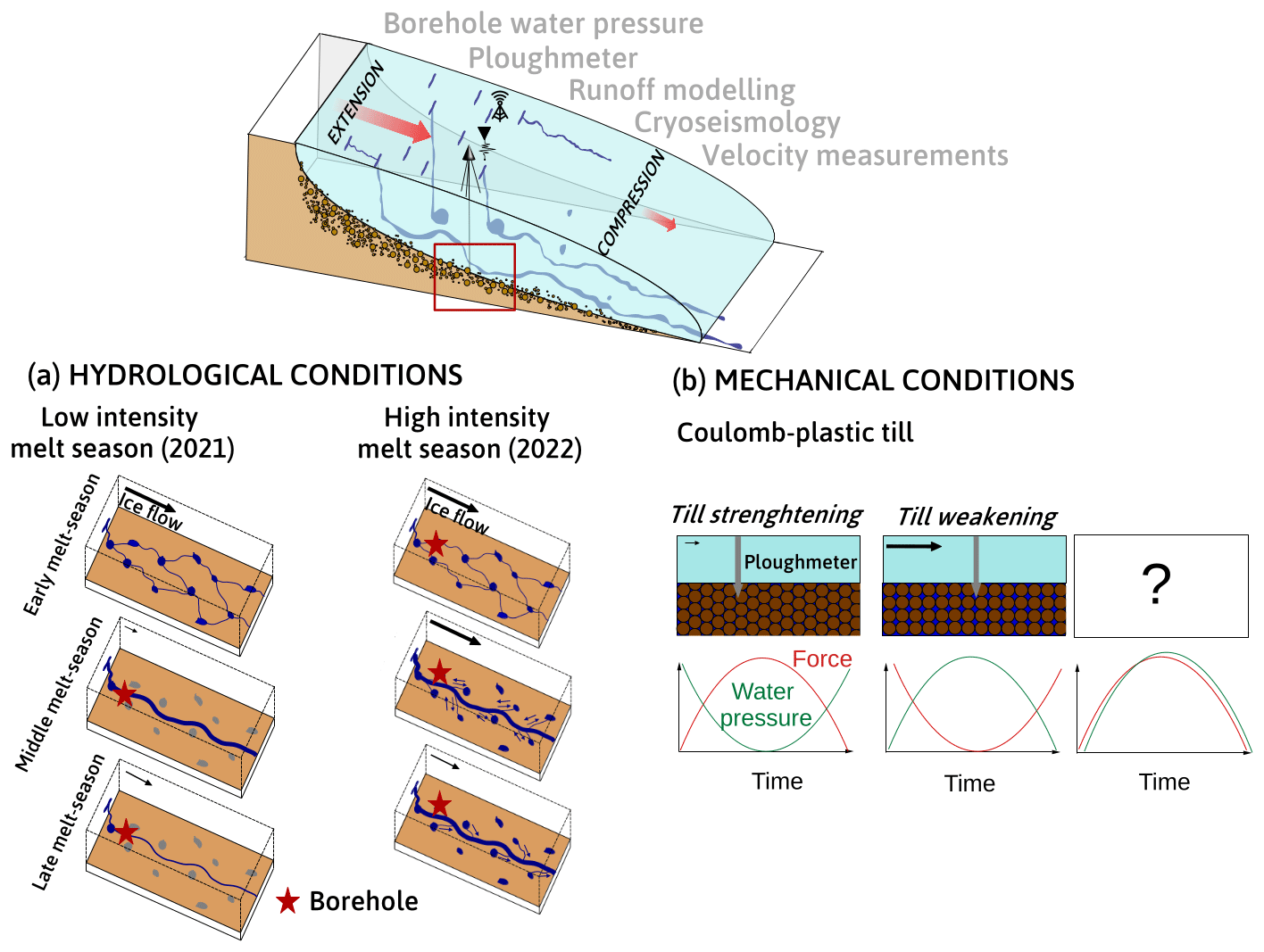
Figure 9 Sketch of the adjustment of hydro-mechanical conditions below Kongsvegen glacier to variations in runoff over the period from June 2021 to August 2022. (a) Hydraulic quantities, i.e., water pressure (p), hydraulic gradient (S), and hydraulic radius (R), used to characterize the evolution of the subglacial drainage system during the short and low-melt-rate season of 2021 and the long and high-melt-rate melt season of 2022. Our findings indicate that during the 2021 season, the subglacial drainage system adapted to runoff changes in steady state, leading to an increase in its capacity over time. However, during the 2022 season, we observed a transient evolution of the drainage system in response to the continued and high input of runoff. As a result, the drainage capacity of the main drainage system was exceeded, causing water to leak into poorly connected areas of the bed increasing the water pressure, thereby triggering speed-up events. (b) The mechanical quantity, i.e., force (F), was used to examine the rheological behavior of the till. The till rheology behaved mainly as a Coulomb plastic material (anti-correlation between p and F) but episodically showed deviating behavior (correlation between p and F), the underlying mechanisms for which remain unclear.

At a seasonal scale, the p–F relationship displays a generally negative slope (Figs. 4e and j and 8a). For a Coulomb plastic material, an increase in pore water pressure results in a decrease in shear strength, which in turn would cause a decrease in force (F; Fig. 9). Furthermore, the observed anti-correlation between water pressure (p) and force (F) is in good agreement with the modeling results of Kavanaugh and Clarke (2006) for a Coulomb plastic material, an interpretation that is in line with the findings of Fischer and Clarke (1994) and Fischer et al. (1998, 2001) at Trapridge Glacier, Storglaciären, and Unteraargletscher, respectively. However, during winter 2021/22, the p–F relationship exhibits a positive slope (Fig. 8a), which is unexpected for Coulomb plastic rheology. Apparent viscous behavior entails a velocity dependency of basal resistance, resulting in a positive p–F relationship. However, we do not observe glacier acceleration during the same period in winter 2021/22.

Over shorter timescales, time series of water pressure (p) and force (F) exhibit complex behavior: correlation (Fig. 8b), anti-correlation (Fig. 8c), and lagging after each configuration occur (Fig. 8d). Applying our interpretation scheme suggests that during episodes similar to those displayed in Fig. 8c, the inverse p–F correlation results from weakening of the sediment at times of high water pressure due to reduced effective pressure and vice versa, as expected for a near-Coulomb rheology (Fig. 9). However, a positive relationship between water pressure (p) and force (F) as pictured in Fig. 8 does not agree with Coulomb plastic rheology. Similar p–F correlations have been observed previously (e.g., Murray and Porter, 2001; Rousselot and Fischer, 2007; Thomason and Iverson, 2008) but not extensively discussed. A range of mechanisms have been proposed to explain such behavior, e.g., the sediments loaded towards their yield point (e.g., Murray and Porter, 2001), the state of the mechanical coupling between the ice and the till and its influence on pore-pressure variations (Iverson et al., 1995; Fischer and Clarke, 1997; Boulton et al., 2001; Mair et al., 2003; Iverson, 2010), and the varying mobilization of the till at depth (e.g., Iverson et al., 1998; Tulaczyk, 1999; Tulaczyk et al., 2001; Truffer et al., 2000; Truffer, 2004). However, a direct explanation of how these mechanisms would explain the correlation between force (F) and water pressure (p) is not straightforward. We further point out that the vertical position of the ploughmeter relative to the till may have changed, e.g., through changes in ploughmeter tilt, but these effects cannot be disentangled from till behavior without further measurements. Such measurements will be subject to future ploughmeter deployments.

6 Conclusions

In this study, we adopt a multi-method, multi-scale analysis to examine the processes governing the responses of Kongsvegen, Svalbard, to changes in runoff over the 2021 and 2022 melt seasons. Our approach involves measuring basal water pressure and the forces exerted on subglacial sediment at the base of a 350 m borehole. These measurements are complemented by surface cryoseismology, which, when combined with runoff modeling, enables us to derive subglacial hydraulic pressure and radius. We then analyze the relationships between these variables across seasonal, multi-day, and diurnal timescales to investigate the complex responses of the subglacial environment to changes in surface melt and precipitation. Here, we synthesize the broad spectrum of relationships between the observed data series in four classes and interpret them in terms of drainage system evolution and till rheology (Fig. 9).

Our data cover two contrasting melt seasons: during the short and less intensive melt season 2021, we suggest that our borehole intersected a well-connected part of the subglacial drainage system, whereas, in the longer and intensive melt season 2022, the borehole recorded characteristics of a poorly connected subdomain of the glacier bed (Fig. 9). Seismological records indicate the existence of an efficient drainage system in both periods. Considering the different footprints of our sensors (e.g., meter-scale sensitivity for the ploughmeter and the water pressure sensor and hundreds of meter-scale sensitivity for the seismic investigation due to the selected frequencies), complementary information can be obtained that allows us to propose a consistent picture of the subglacial environment. The apparent disagreement between seismic data and borehole-sensed pressure records can be explained by the spatial heterogeneity of the subglacial drainage system, supporting the concept of a discontinuous, spatially heterogeneous drainage system (Fig. 9; Andrews et al., 2014; Hoffman et al., 2016; Nanni et al., 2021; Rada Giacaman and Schoof, 2023).

The relationship between the force experienced by the ploughmeter and the water pressure reveals complex behavior. As expected, the till behaves mostly as a Coulomb plastic material. In the future, monitoring instrument vertical position could help disentangle instrument behavior from till behavior, and assessments of changes in till properties using seismic noise interferometry (Zhan, 2019) over a large area could complement the local ploughmeter record.

By constraining the spatial and temporal extents of our investigation, this study investigated local subglacial hydro-mechanical conditions rather than explored the multi-annual and likely large-scale processes responsible for the surge buildup. We show the importance of a multi-sensor multi-scale approach to study the complex variations of hydro-mechanical conditions in response to runoff changes. Such an approach may also be beneficial for studying the dynamics of other transient geological systems that are characterized by the buildup and evolution of internal states. These states may reach critical thresholds causing instabilities over different scales from short-lived events to large-scale events by destabilization as exemplified in many geohazards such as glacial surges or collapses, volcanic eruptions, landslides, or earthquakes.

Appendix A: Full time series

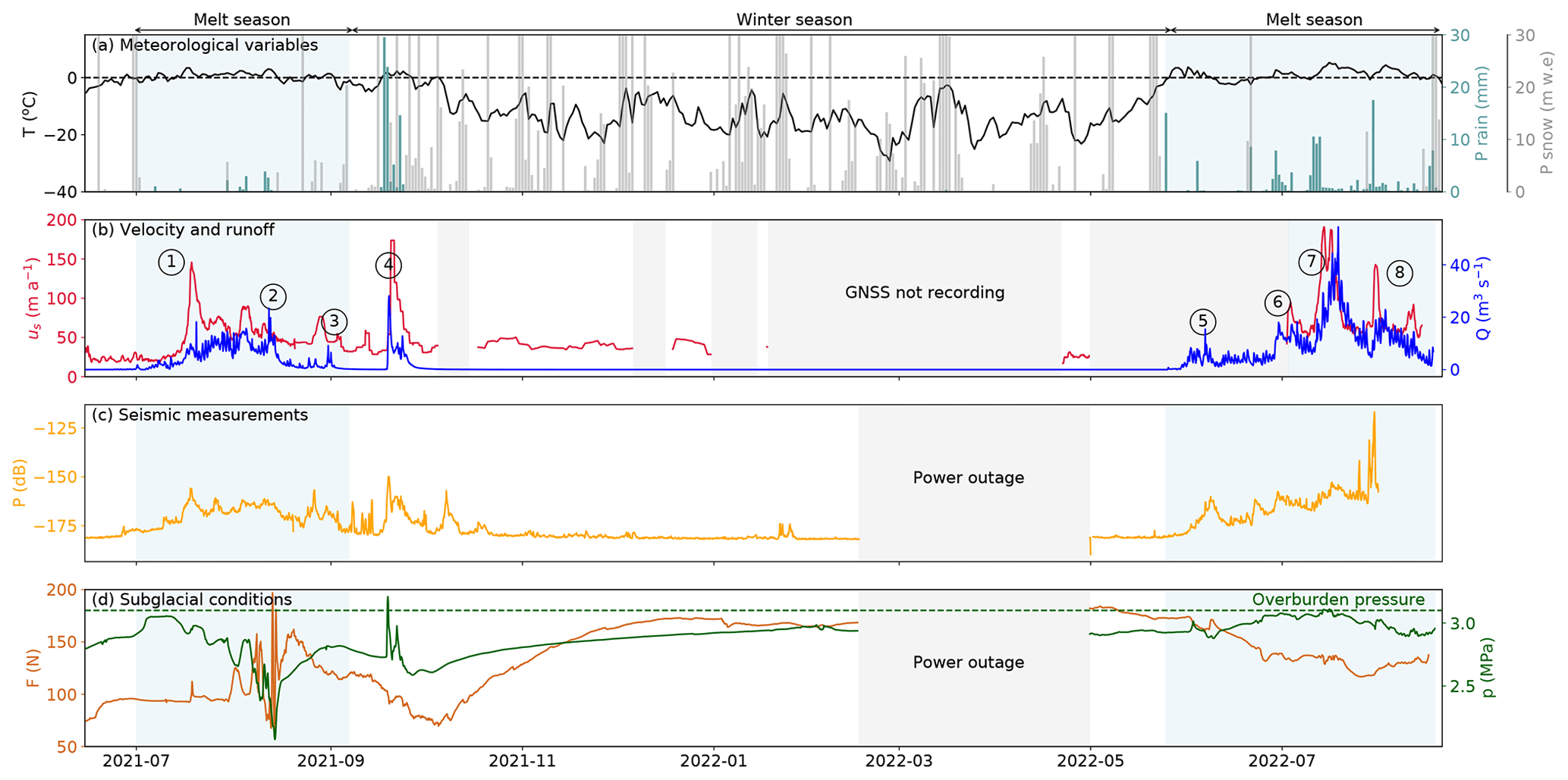
Figure A1 Time series of physical quantities measured from spring 2021 to summer 2022. (a) Temperature (black line), precipitation (light blue bars) from CARRA/AROME-Arctic, and relative glacier surface height (gray line) from CryoGrid simulations (Schmidt et al., 2023). The three variables are extracted for the closest grid point of the borehole. In 2022, the surface height is negative, which corresponds to ice melt. (b) Modeled runoff (blue line) and glacier surface velocity measured (red line). Circled numbers refer to different episodes described in the main text. (c) Turbulent-water-flow-induced seismic power recorded at the surface of the glacier in the 3–10 Hz frequency band (yellow line). (d) Borehole water pressure (green line) and force acting on the ploughmeter (dark red line). Blue shaded areas represent the melt seasons. Gray shaded areas represent periods of missing data.

Appendix B: Pre-processing of the time series

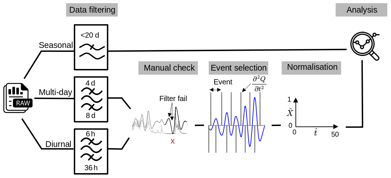
Figure B1 Pre-processing workflow applied to the time series. The original time series (see Fig. 3 below) have been filtered at three timescales. The multi-day and diurnal filtered data have been inspected against the unfiltered data to remove spurious artifacts that can be created by the filtering technique (see also Appendix G, Fig. G1). We then segmented the recorded data into multiple events and normalized the magnitude and duration of each.

Appendix C: Surface velocity data

The velocity record presented in this study combines two different GNSS records. One of the GNSS stations is positioned at stake 6 (KNG-6: 13.15153° E 78.78067° N) and the other one at stake 7 (KNG-7: 13.23962° E 78.76770° N). In Fig. C1, we present the two datasets that have been combined. We apply a 1-week moving median for KNG7 velocity to smooth the record especially during the winter period when the velocities are low and thus the daily velocity derivation is less accurate.

Figure C1 Velocity data series from GNSS stations KNG6 (red curve) and KNG7 (blue curve).

Appendix D: Events

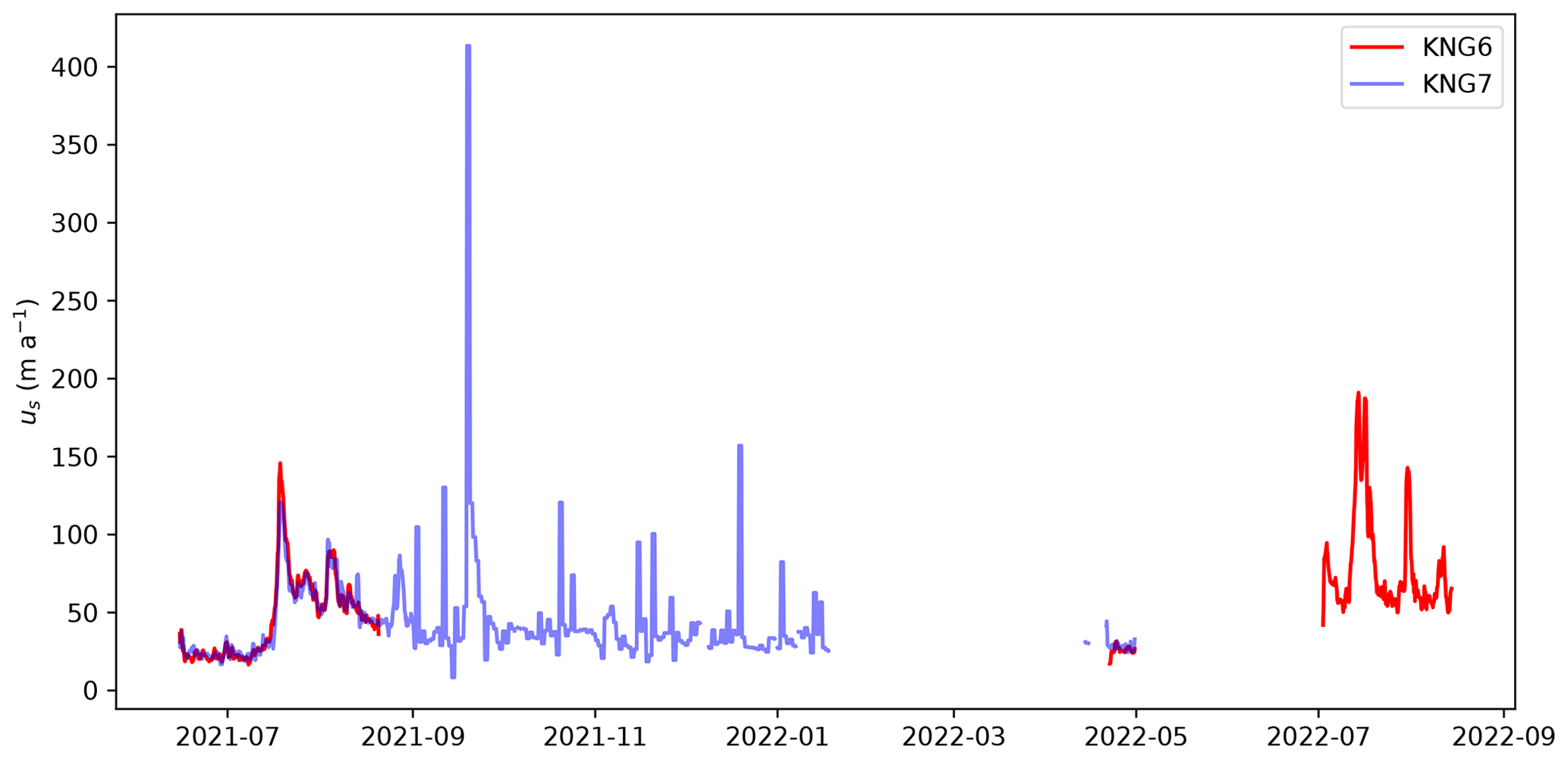
Table D1 Description of the 12 multi-day timescale events during the melt season 2021.

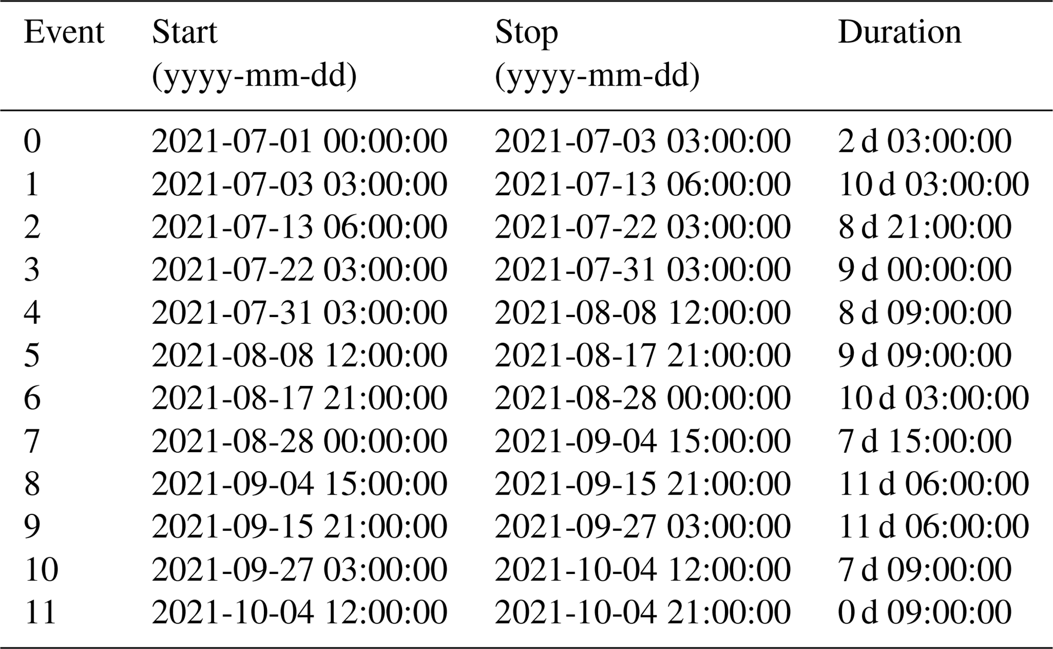
Table D2 Description of the eight multi-day timescale events during the melt season 2022.

Table D3 Description of the 96 diurnal timescale events during the melt season 2021.

Table D4 Description of the 85 diurnal timescale events during the melt season 2022.

Appendix E: Spectrogram

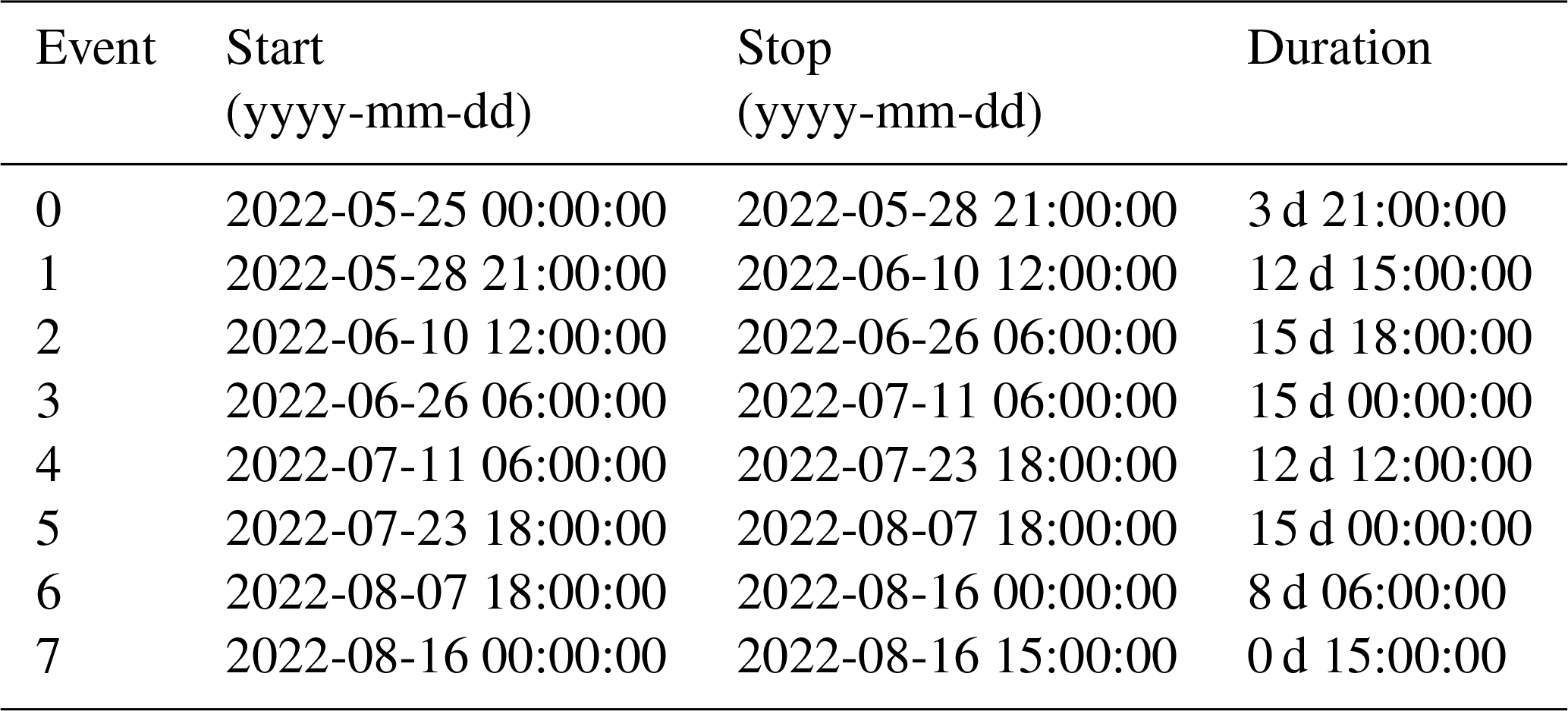
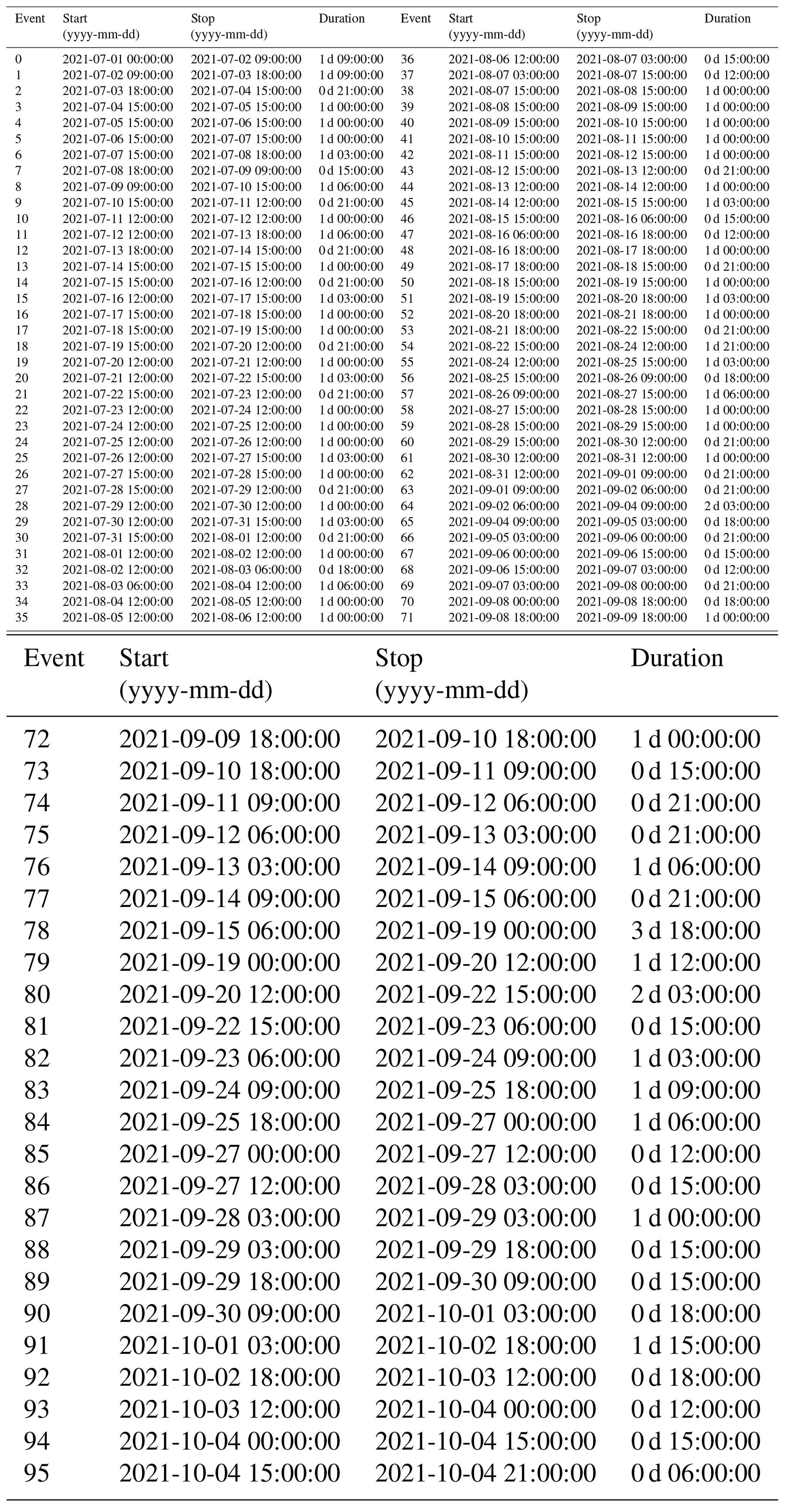
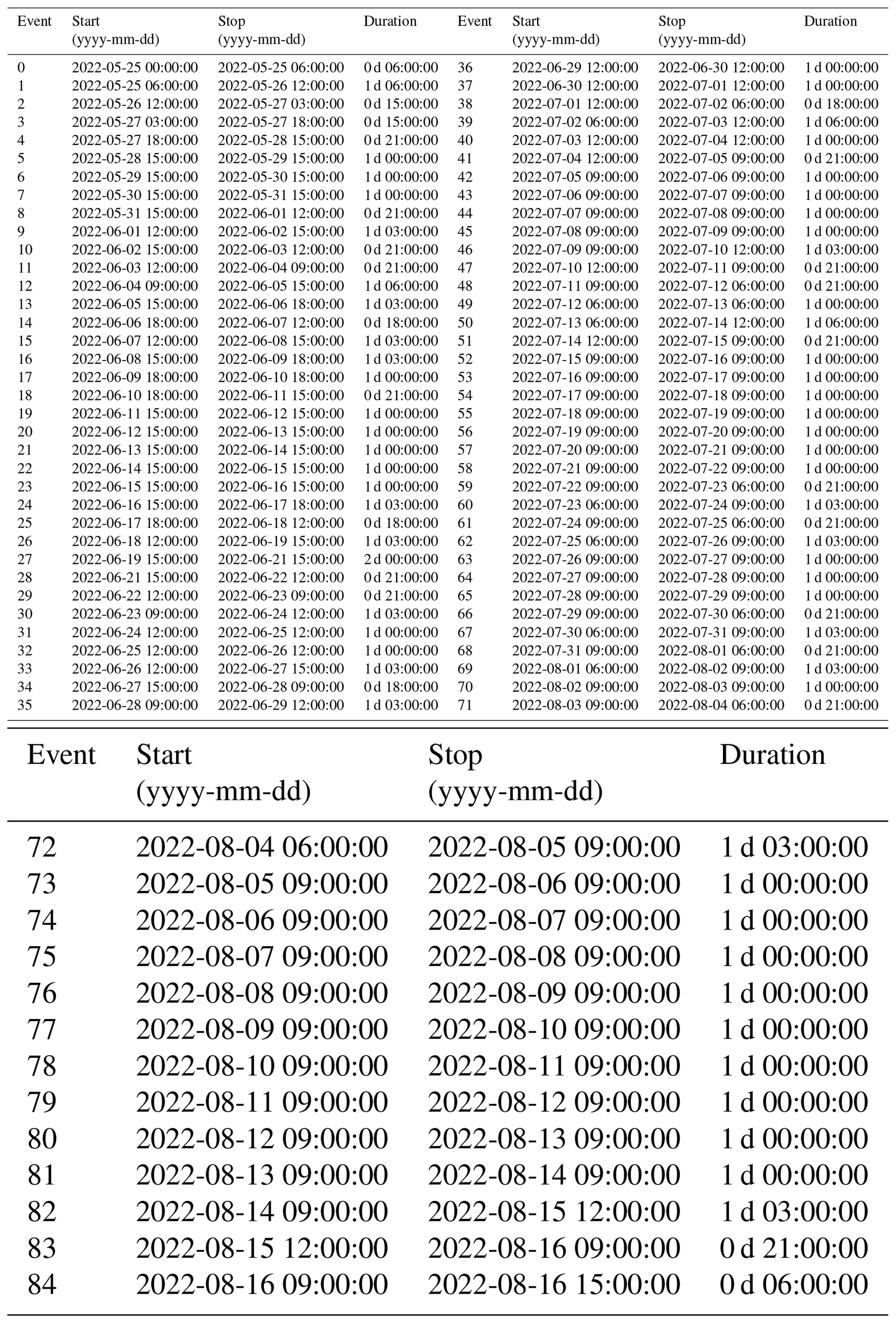
Large seasonal changes in turbulent-water-flow-induced seismic power, and P values are observed within the 3–10 Hz frequency range, in which P is higher by more than 2 orders of magnitude during the melt season (mid-May to September) compared to winter (Fig. E1). Changes in P are also observed within the 10–20 Hz frequency range, with P during the melt season being about an order of magnitude larger than in winter (Fig. E1).

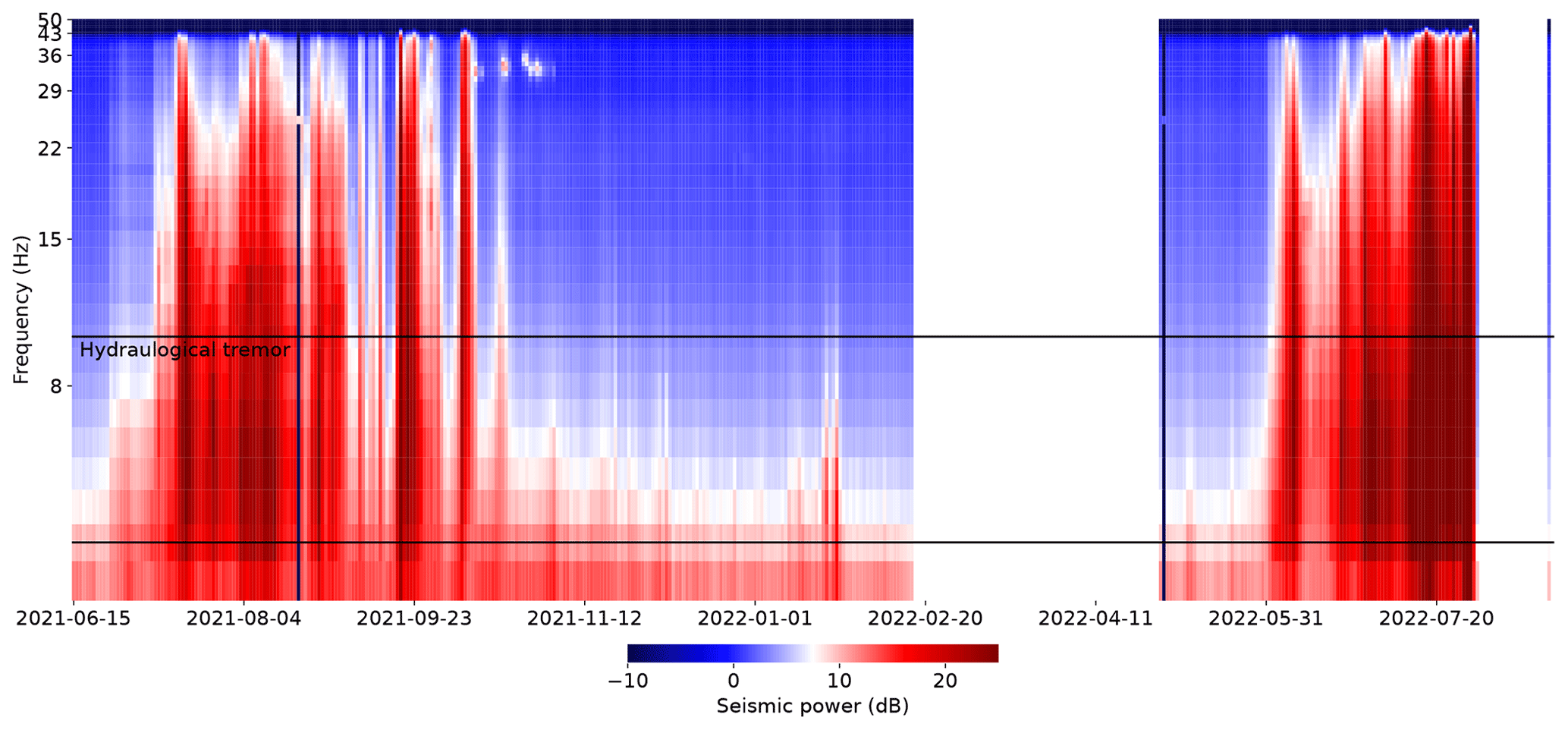
Figure E1 Spectrogram of the observed seismic power P as a function of time on the x axis and frequency on the y axis. Colors represent seismic power on a decimal logarithmic scale. White bands are data gaps. The two black lines delineate the frequency band between 3 and 10 Hz that we used in this study.

Appendix F: Metrics used in the classification

Figure F1 provides a visual representation of the metrics used to classify the events.

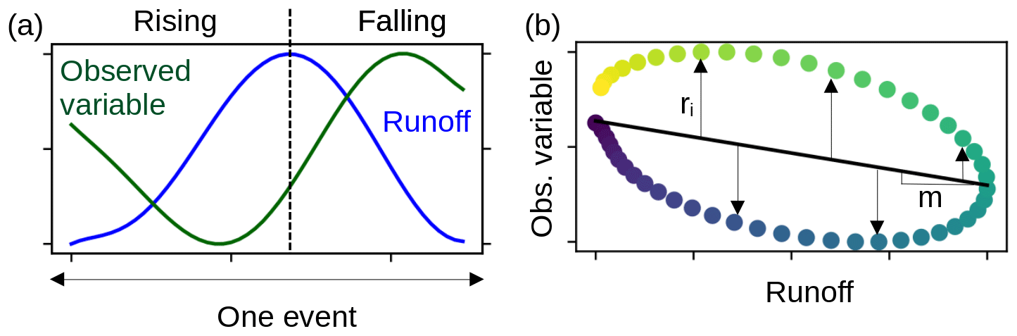
Figure F1 Description of the metrics used to classify the events. (a) Description of one event with the rising and falling part of the runoff to calculate the hysteresis θ. (b) The linear fit used to calculate the residual sum of squares RSS and its slope, m.

Appendix G: Band-pass-filtered time series

We have filtered the original time series to determine the different frequency signatures separately. For the seasonal scale, we have applied a low-pass filter with a cutoff at 20 d (Fig. G1a). For the multi-day scale, we have applied a band-pass filter between 4–8 d (Fig. G1b). For the daily timescale, we have applied a band-pass filter between 6–36 h (Fig. G1b).

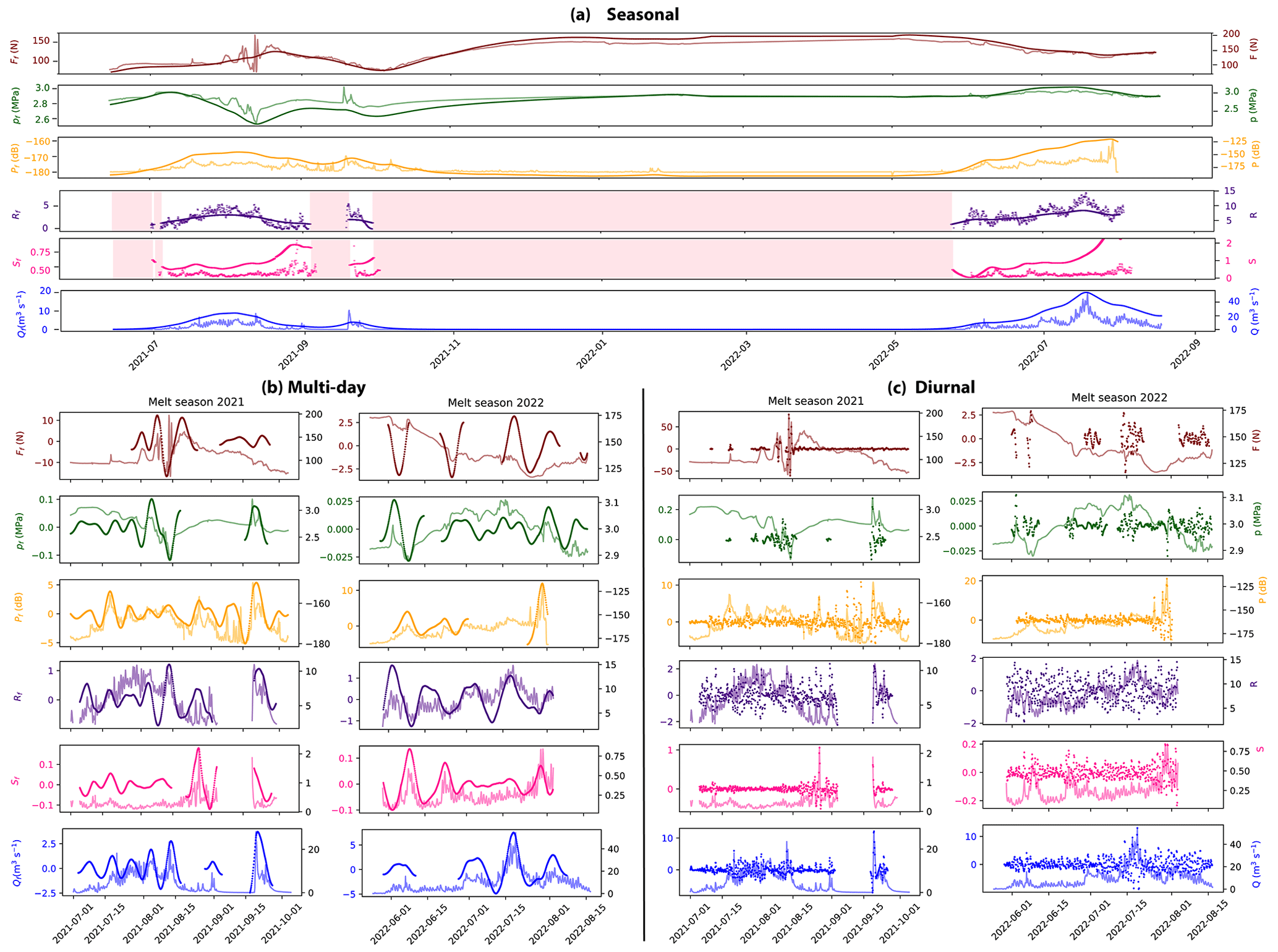
Figure G1 Band-pass filtered series for (a) seasonal (>20 d), multi-day (4–8 d), and diurnal (6 to 36 h) timescales. For the last two series, we have computed the band-pass time series for the melt season time period only.

Appendix H: Frequency content of the time series between 6 h and 10 d

Figure H1 shows the frequency content of all variables over the recording period between a period of 6 h and a period of 10 d. While the force and the water pressure have only episodic frequency content on the scale of 1 d, the other variables exhibit longer periods with variations on that timescale but still concentrated during the melting season.

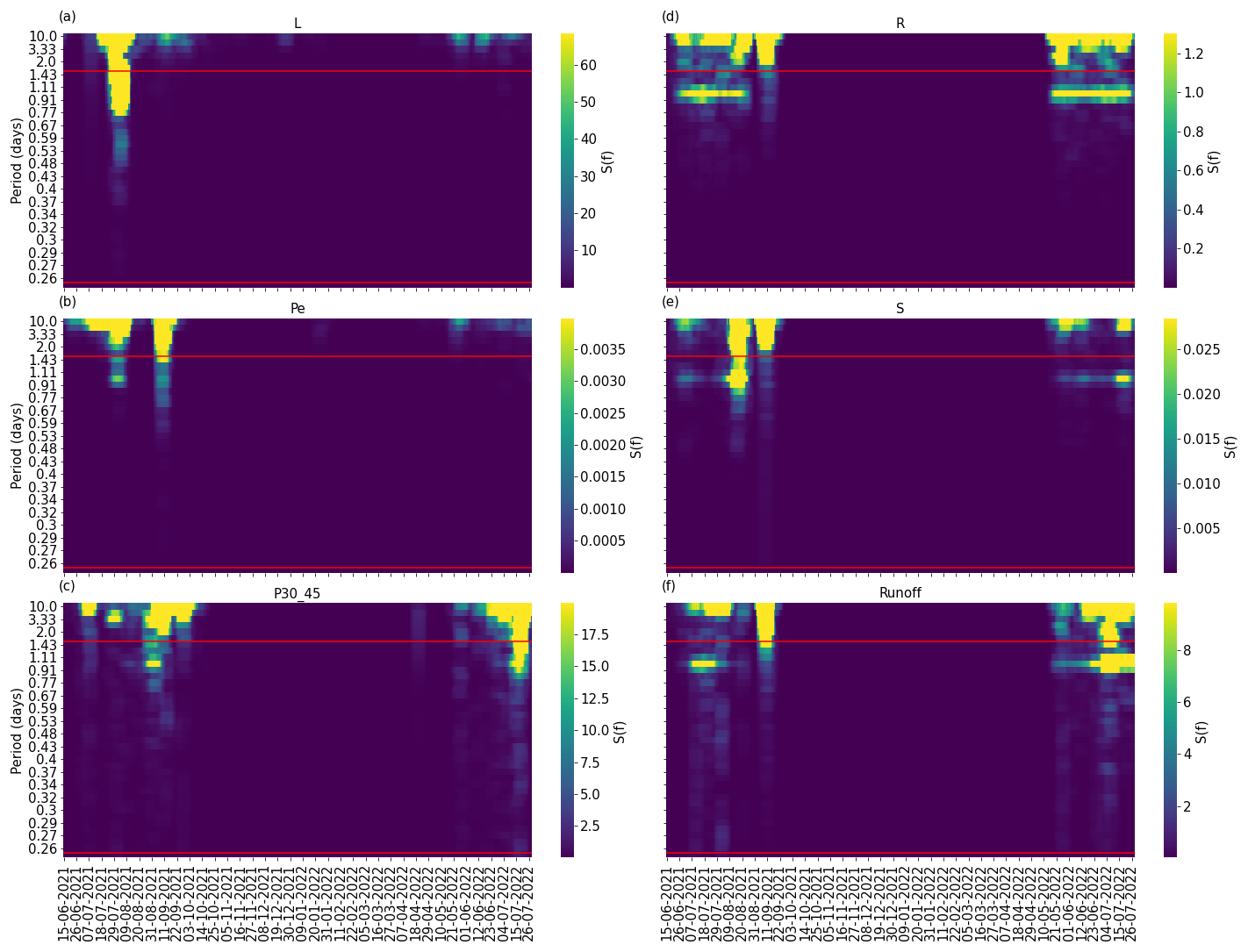
Figure H1 Frequency content intensity for all the variables between 6 h an 10 d over the year. The red lines delineate the diurnal frequency content (between 6 and 36 h).