the Creative Commons Attribution 4.0 License.
the Creative Commons Attribution 4.0 License.
 | 25 Jun 2024
Ice-shelf freshwater triggers for the Filchner–Ronne Ice Shelf melt tipping point in a global ocean–sea-ice model
Carolyn Branecky Begeman
Xylar S. Asay-Davis
Darin Comeau
Alice Barthel
Stephen F. Price
Jonathan D. Wolfe
Some ocean modeling studies have identified a potential tipping point from a low to a high basal melt regime beneath the Filchner–Ronne Ice Shelf (FRIS), Antarctica, with significant implications for subsequent Antarctic ice sheet mass loss. To date, investigation of the climate drivers and impacts of this possible event have been limited because ice-shelf cavities and ice-shelf melting are only now starting to be included in global climate models. Using a global ocean–sea-ice configuration of the Energy Exascale Earth System Model (E3SM) that represents both ocean circulations and melting within ice-shelf cavities, we explore freshwater triggers (iceberg melt and ice-shelf basal melt) of a transition to a high-melt regime at FRIS in a low-resolution (30 km in the Southern Ocean) global ocean–sea-ice model. We find that a realistic spatial distribution of iceberg melt fluxes is necessary to prevent the FRIS melt regime change from unrealistically occurring under historical-reanalysis-based atmospheric forcing. Further, improvement of the default parameterization for mesoscale eddy mixing significantly reduces a large regional fresh bias and weak Antarctic Slope Front structure, both of which precondition the model to melt regime change. Using two different stable model configurations, we explore the sensitivity of FRIS melt regime change to regional ice-sheet freshwater fluxes. Through a series of sensitivity experiments prescribing incrementally increasing melt rates from the smaller, neighboring ice shelves in the eastern Weddell Sea, we demonstrate the potential for an ice-shelf melt “domino effect” should the upstream ice shelves experience increased melt rates. The experiments also reveal that modest ice-shelf melt biases in a model, especially at coarse ocean resolution where narrow continental shelf dynamics are not well resolved, can lead to an unrealistic melt regime change at downstream ice shelves. Thus, we find that remote connections between melt fluxes at different ice shelves are sensitive to baseline model conditions. Our results highlight both the potential and the peril of simulating prognostic Antarctic ice-shelf melt rates in a low-resolution global model.
- Article
(11537 KB) - Full-text XML
- BibTeX
- EndNote


Mass loss from the Antarctic ice sheet is the most uncertain contributor to projections of future sea-level rise due to the potential for destabilization of marine-terminating sectors of the ice sheet (Church et al., 2013). Ice shelves restrain the flow of the grounded ice behind them, and thinning of ice shelves due to intensified melting from the ocean below leads to flow acceleration and increased mass loss of grounded ice (Joughin et al., 2012; Gudmundsson, 2013; Reese et al., 2018; Gudmundsson et al., 2019; Zhang et al., 2020). Thus, changes in ocean conditions within the cavities beneath ice shelves can strongly control ice-sheet evolution.
Ice-shelf cavities around Antarctica can be classified as “cold” or “warm” based on the absence or presence of modified Circumpolar Deep Water, resulting in ice shelves with low (𝒪(1 m yr−1)) or high melt rates (𝒪(10 m yr−1)), respectively (Jacobs et al., 1992; Dinniman et al., 2016; Jenkins et al., 2016). Cold cavities, such as the one below the Filchner–Ronne Ice Shelf (FRIS; Fig. 1), may transition to warm conditions through the intrusion of modified Circumpolar Deep Water or modified Weddell Deep Water (mWDW) in the Weddell Sea (Hellmer et al., 2012). For FRIS, some modeling studies have shown the existence of a tipping point from a stable, cold state to a stable, warm state when the intrusion of mWDW becomes amplified by invigorated overturning circulation (Hellmer et al., 2012; Thoma et al., 2015; Hellmer et al., 2017; Hazel and Stewart, 2020; Daae et al., 2020; Haid et al., 2023; Mathiot and Jourdain, 2023). Once triggered, the switch in regimes with respect to ocean cavity temperature and FRIS basal melt rates is rapid (occurring over 1 to 2 decades) and remains stable even after the removal of the perturbation that triggered it (Hellmer et al., 2017; Hazel and Stewart, 2020) or exhibits reversible behavior with hysteresis (Haid et al., 2023).
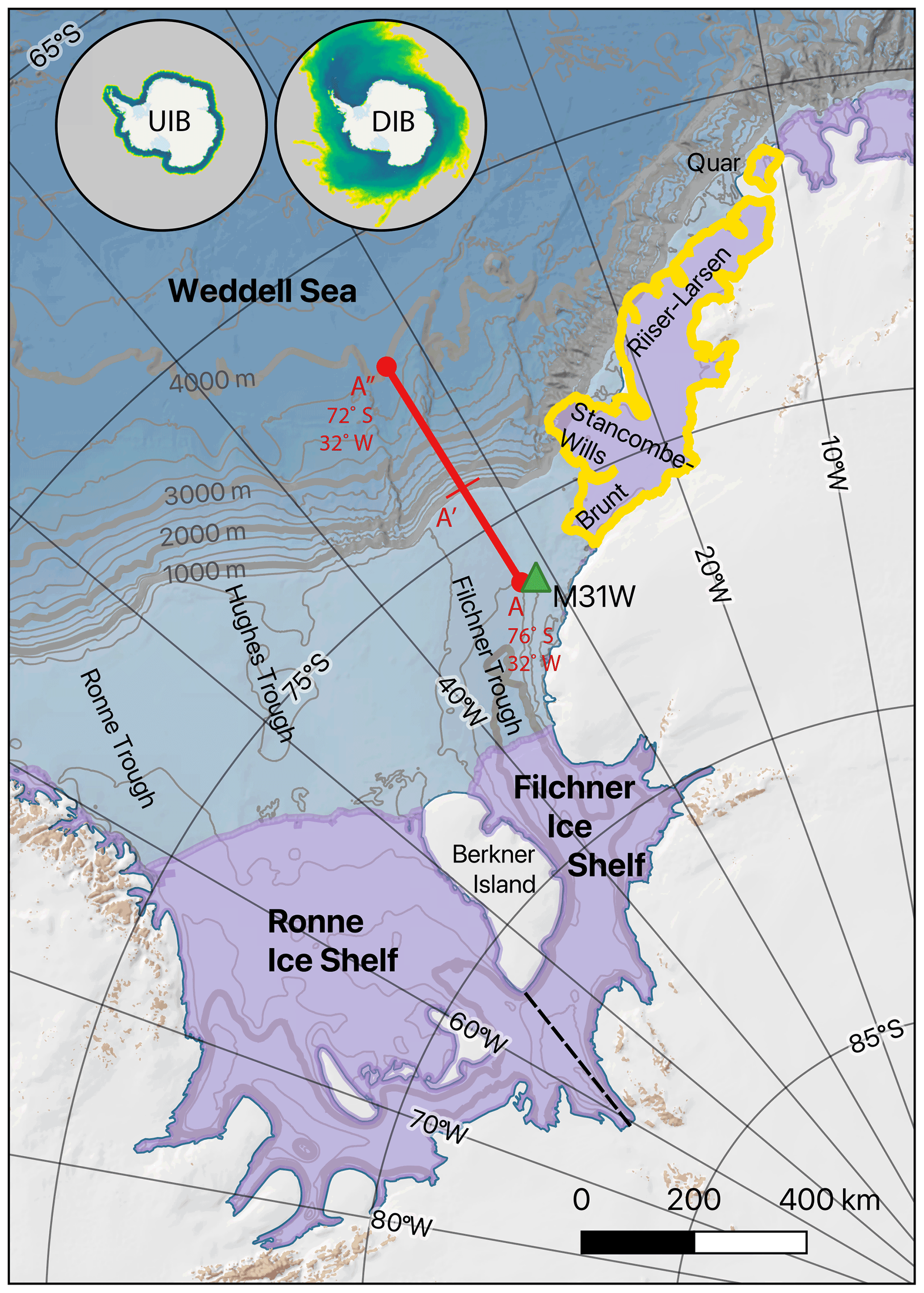
Figure 1Map of the southern Weddell Sea and Filchner–Ronne Ice Shelf. The dotted black line indicates the boundary between Filchner and Ronne ice shelves used in this study. The yellow outline indicates eastern Weddell Sea ice shelves under which prescribed melt rates are applied, as described in Sect. 2.3. The green triangle is the location of the M31W mooring described by Ryan et al. (2017) that is used for comparison in Fig. 9. The red line is the transect used in Fig. 10 (A-A′) and in Fig. 11 (A′-A′′). Inset maps show the relative distribution of iceberg melt flux on a log scale for the uniform iceberg (UIB) and data iceberg (DIB) configurations. See Comeau et al. (2022, Fig. 2) for details. Gray lines are bathymetry contours (Dorschel et al., 2022). The base map is from Quantartica (Matsuoka et al., 2018).
Under some greenhouse gas emission scenarios, some climate models project that the FRIS tipping point may be crossed in the late 21st century (Hellmer et al., 2012, 2017; Timmermann and Hellmer, 2013), while in other models the tipping point is not reached regardless of emission scenario (Naughten et al., 2018). Daae et al. (2020) showed that this tipping point can be reached through significant freshening of Dense Shelf Water (DSW) and shoaling of the thermocline at the continental slope. These conditions reduce the density contrast between the continental shelf and the open ocean, leading to inflow of mWDW that was otherwise blocked by DSW (Daae et al., 2020; Hellmer et al., 2017; Haid et al., 2023; Mathiot and Jourdain, 2023). At the same time, recent studies have demonstrated that ocean properties and ice-shelf melt rates can be affected by remote conditions via the Antarctic Slope Current (Nakayama et al., 2014, 2020; Gille et al., 2016; Thompson et al., 2018; Bull et al., 2021; Dawson et al., 2023). As such, ice-shelf basal meltwater can have far-reaching impacts as it is advected along the coast by the Antarctic Coastal Current, modifying DSW properties, affecting mWDW access to the continental shelf, and impacting Antarctic Bottom Water production (Nakayama et al., 2014, 2020; Silvano et al., 2018; Thompson et al., 2018).
To date, the ocean models that have been used to understand the mechanisms affecting Antarctic ice-shelf basal melt, including the FRIS tipping point, have largely been regional in extent and/or are uncoupled from atmosphere models. In contrast, Earth system models are more useful for future projections but generally have coarse resolution and more simplified parameterizations of physical processes. The Energy Exascale Earth System Model (E3SM) is one of the first Earth system models to include ice-shelf cavities and prognostic melt fluxes (Jeong et al., 2020; Comeau et al., 2022).
Here, we present the results of E3SM ocean and sea-ice simulations at low resolution driven by historical atmospheric reanalyses, focusing on FRIS tipping point behavior and the model conditions leading to it. We find that the typical treatment of Antarctic freshwater fluxes in climate models, a distribution that is uniform along the Antarctic coast and confined to 𝒪(100 km) from the coast, quickly leads the E3SM ocean–sea-ice model to cross the FRIS melt tipping point. We attribute this in part to the iceberg melt term; switching to an iceberg melt climatology dataset avoids the tipping point and allows E3SM to model FRIS sub-shelf circulations and melting well. However, a strong regional fresh bias and a weak Antarctic Slope Front (ASF) remain, which may precondition the model to prematurely reach the tipping point under future forcing. Modifying the default mesoscale eddy-mixing parameterization significantly reduces these biases but fails to eliminate excessive melting of smaller ice shelves in the eastern Weddell Sea where the continental shelf is narrow. Motivated by these elevated proximate ice-shelf melt fluxes and the sensitivity of the modeled FRIS melt regime to freshwater flux, we conduct a series of experiments wherein eastern Weddell Sea ice shelves melt at the above-observed rates. We find that melt fluxes representative of a partial transition from cold- to warm-cavity conditions in this adjacent region are sufficient to trigger the FRIS melt regime change, with the threshold being sensitive to the baseline model state. We discuss some challenges these remote connections between ice-shelf melt fluxes create in a low-resolution global model and the extent to which the model results suggest the potential for a real-world ice-shelf melt domino effect.
E3SM (Leung et al., 2020; Golaz et al., 2019) is an Earth system model with coupled model components for the atmosphere (Rasch et al., 2019), oceans (Petersen et al., 2019), sea ice (Turner et al., 2021), land (Bisht et al., 2018), rivers (Li et al., 2015), and ice sheets (Hoffman et al., 2018). Notable aspects of E3SM are the ability of all components to use variable resolution meshes and formulation to run on advanced supercomputing architectures with the ultimate goal of exascale computing performance (Leung et al., 2020). E3SM v1 simulations were organized into three science simulation campaigns: Water Cycle (v1.0; Golaz et al., 2019), Biogeochemistry (v1.1; Burrows et al., 2020), and Cryosphere Systems (v1.2; Comeau et al., 2022), the last of which is used here. The E3SM v1.2 Cryosphere configuration introduced two notable E3SM capabilities for realistically representing freshwater fluxes from Antarctica into the ocean (Comeau et al., 2022). The first is the addition of Antarctic ice-shelf cavities and prognostic ice-shelf basal melt fluxes into the ocean model. The second is the representation of iceberg melt fluxes through a prescribed monthly climatology based on the reanalysis of Merino et al. (2016) instead of them being applied uniformly around the Antarctic coast following the Coordinated Ocean-ice Reference Experiment – Phase II with inter-annual forcing (CORE-II IAF) protocol (Large and Yeager, 2008) as had been done previously. In this study, we use the ocean and sea-ice components of E3SM forced by historical atmospheric reanalysis.
2.1 Ocean and sea-ice model description
The ocean and sea-ice components of E3SM are the Model for Prediction Across Scales-Ocean (MPAS-Ocean; Petersen et al., 2019) and the Model for Prediction Across Scales-Sea Ice (MPAS-Sea ice; Turner et al., 2021). The models are built on a common framework (as is the ice sheet model MPAS-Albany Land Ice; Hoffman et al., 2018) that defines spherical or planar centroidal Voronoi meshes (Ringler et al., 2013), commonly used geophysical operators, input/output libraries, and parallelization methods (Message Passing Interface and openMP). MPAS-Ocean uses a finite volume discretization on a staggered C-grid of a three-dimensional hydrostatic Boussinesq approximation to the incompressible-fluid-flow equations. MPAS-Sea ice uses a combination of finite volume and finite element methods (Turner et al., 2021) to describe the flow of ice in a continuum approximation with elastic–viscous–plastic rheology (Hunke and Dukowicz, 1997) and complete thermodynamics (Turner et al., 2013; Turner and Hunke, 2015). Both models use explicit forward time stepping with subcycling of some fast processes.
Extensive details of MPAS-Ocean can be found in Petersen et al. (2019) and in Comeau et al. (2022) and associated references, but some key aspects are summarized here. MPAS-Ocean employs a z′ vertical coordinate (Adcroft and Campin, 2004; Petersen et al., 2015) that is modified beneath ice shelves so that the top layer follows the ice draft, and layer thicknesses are adjusted to mitigate pressure-gradient errors (Comeau et al., 2022). The calculation of ice-shelf basal fluxes of mass, heat, and salinity uses a standard parameterization of boundary layer turbulence (Hellmer and Olbers, 1989; Holland and Jenkins, 1999) with a velocity-dependent transfer coefficient for heat and salt that is spatially uniform and calibrated to Antarctic-wide observations of ice-shelf basal melt rate (Rignot et al., 2013). For E3SM v1.2, ice-shelf cavities have a fixed geometry and do not evolve as melt occurs.
2.2 Baseline simulation configurations
The simulations presented here use the E3SM v1 low-resolution global ocean–sea-ice mesh (EC60to30 in Petersen et al., 2019) that features 60 km resolution at mid latitudes refined to 30 km in equatorial and high-latitude regions. Resolution in the Southern Ocean ranges from about 35 km at the coast to 50 km near the Subtropical Front. There are 60 vertical levels in the ocean mesh, ranging from 10 m thickness at the surface to 250 m at depth. The model uses a time step of 30 min. The E3SM v1.2 Cryosphere configuration is capable of being run both in a configuration with coupling between atmosphere, land, river, ocean, and sea-ice components (Comeau et al., 2022) and in one with ocean and sea ice only. In this study, we only present results from the ocean and sea-ice configuration. This configuration uses the atmospheric forcing and prescribed terrestrial freshwater fluxes from the Coordinated Ocean-ice Reference Experiment Phase II with interannual forcing (CORE-II IAF; Large and Yeager, 2008) together with sea-surface-salinity restoring to a monthly climatology. Sea-surface-salinity restoring is applied everywhere in the global ocean, with the exception of beneath sea ice and inside ice-shelf cavities, and uses a piston velocity of 50 m yr−1, which can be interpreted as a timescale of 1 year for a surface layer depth of 50 m. The global mean is removed to avoid a spurious net source or sink of salt. As in other studies, the 62-year forcing cycle of 1948–2009 is repeated multiple times.
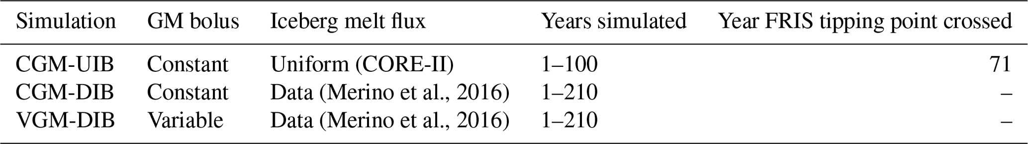
(Merino et al., 2016)(Merino et al., 2016)Table 1Table of baseline simulations conducted for this study. All simulations include prognostic ice-shelf melt fluxes and use the CORE-II IAF atmospheric forcing. The GM bolus coefficient is either constant or variable. Iceberg melt fluxes are either prescribed uniformly around the coast following the CORE-II protocol or are represented by the Merino et al. (2016) climatology.
At low resolution, MPAS-Ocean uses the Gent–McWilliams parameterization (Gent and Mcwilliams, 1990) for the horizontal mixing induced by unresolved mesoscale eddies. The standard application in E3SM v1 uses a spatially and temporally constant bolus coefficient, which has a value of 600 m2 s−1 (Petersen et al., 2019) for simulations with prescribed atmospheric forcing. However, early E3SM v1 ocean simulations indicated that the use of a constant bolus coefficient value led to weak ocean circulation (Petersen et al., 2019). An alternative implementation was added to MPAS-Ocean, here referred to as “variable GM”, that scales the bolus coefficient by the in situ stratification, resulting in a spatially and temporally variable value (Danabasoglu and Marshall, 2007; Comeau et al., 2022). Details of variable GM implementation and its effects on the Southern Ocean in MPAS-Ocean were described by Comeau et al. (2022).
We present results from three model configurations of increasing sophistication (Table 1), all with active ice-shelf melt fluxes.
-
CGM-UIB. The CGM-UIB run uses the Gent–McWilliams parameterization with a constant bolus coefficient and a uniform distribution of iceberg melt around the coast of Antarctica with a Gaussian smoothing spread over 300 km (Fig. 1, inset). The total magnitude of iceberg melt flux applied is 1187 Gt yr−1, the approximate observed total calving flux for Antarctica (Rignot et al., 2013; Depoorter et al., 2013). This treatment of iceberg melt fluxes is equivalent to 45 % of the Antarctic freshwater flux prescribed by CORE-II IAF. Spreading Antarctic freshwater fluxes around the coast is also traditionally how freshwater fluxes are represented in many climate models, including in the E3SM default v1.0 configuration (Petersen et al., 2019; Golaz et al., 2019). This run was stopped at model year 100 after the FRIS melt regime tipping point was crossed in year 71.
-
CGM-DIB. The CGM-DIB run uses the same Gent–McWilliams parameterization with a constant bolus coefficient and applies the Merino et al. (2016) data iceberg melt flux climatology (Fig. 1, inset). Thus, it is identical to CGM-UIB but with the application of a more realistic iceberg melt flux distribution (Comeau et al., 2022, their Fig. 2d).
-
VGM-DIB. The VGM-DIB run uses the Gent–McWilliams parameterization with a spatially and temporally varying bolus coefficient and applies the Merino et al. (2016) data iceberg melt flux climatology. It is identical to CGM-DIB but with the improved treatment of the Gent–McWilliams parameterization discussed above.
We define FRIS melt regime change as an increase in mean FRIS basal melt rate exceeding 2 times its observed values sustained for the duration of the simulation. Since previous studies have identified this regime change as being associated with tipping points (Hellmer et al., 2017; Hazel and Stewart, 2020), we assume that tipping points have been reached by simulations that undergo a FRIS melt regime change.
For the CGM-DIB and VGM-DIB runs that avoided the FRIS melt regime tipping point, the oceanographic conditions in the third CORE-II cycle were similar to the second CORE-II cycle. This was considered sufficient spin-up, and these runs were stopped at model year 210. This end year was chosen as it allowed a complete 62-year cycle of forcing after year 140, which is used as a branch point for additional runs as described in the following section.
2.3 Eastern Weddell prescribed melt branch simulations
As discussed below, our baseline simulations indicate that the FRIS melt regime and the associated eastern Weddell Sea continental shelf water mass properties are highly sensitive to land-ice freshwater flux. They also a reveal a significant high-melt-rate bias in the ice shelves northeast of FRIS, which is upstream of FRIS via the coastal current. Furthermore, Kusahara and Hasumi (2013) and Thoma et al. (2010) found that the eastern Weddell Sea continental shelf was one of the regions most sensitive to intrusion of modified Circumpolar Deep Water under surface warming due to the narrowness of the continental shelf. To probe the potential sensitivity of modeled FRIS melt rates to this upstream ice-shelf melt bias in combination with ocean mean state biases, we conduct an ensemble of partially prescribed melt experiments that branch off of the CGM-DIB and VGM-DIB baseline simulations. In each branch run, we prescribe a spatially and temporally uniform melt rate for the ice shelves in the eastern Weddell Sea region, encompassing the Brunt, Stancomb-Wills, Riiser-Larsen, and Quar ice shelves (28 to 10° W; Fig. 1). Collectively, these ice shelves occupy an area of 77 380 km2 on our mesh, which is similar to the surveyed area of 87 511 km2 for these ice shelves (Rignot et al., 2013), given the discretization at this coarse resolution. Ice-shelf basal melt fluxes are prognostic for all ice shelves, including FRIS, outside of this region. We perform branch runs from both the CGM-DIB and VGM-DIB simulations to explore the relative sensitivity of these two model configurations to perturbations in ice-shelf melt fluxes.
The ensemble of sensitivity experiments is comprised of prescribed melt rates in the eastern Weddell Sea region of 0.58, 1, 2, 4, 8, and 16 m yr−1 (corresponding to a 40.8, 70.4, 140.8, 281.7, 563.3, or 1126.7 Gt yr−1 total melt flux, respectively). The low-end value represents the mean melt rate for this region simulated by the CGM-DIB baseline run, slightly higher than the mean melt rate for the VGM-DIB baseline run of 0.46 m yr−1. The lower values in the range are comparable to the interannual melt rate variability of 0.62 m yr−1, relative to a long-term average of 0.67 m yr−1, as observed by Lauber et al. (2023) at Fimbulisen Ice Shelf in this region. The high-end value is comparable to the “warm shelf” conditions at the Pine Island and Thwaites ice shelves, which have average melt rates of 14 and 27 m yr−1, respectively (Adusumilli et al., 2020). It is also comparable to the modeled melt rates for these ice shelves from the future high-end emissions scenario considered by Mathiot and Jourdain (2023). The prescribed melt rates at values between those characteristic of warm- and cold-cavity conditions could be considered approximate states with intermediate cross-shelf heat fluxes associated with mWDW. They also provide model insight into the real-world potential for remote influence between ice-shelf melt fluxes at different ice shelves. Where we prescribe melt fluxes, we set the associated latent heat flux to zero; because the ambient temperature and salinity beneath the ice shelves are generally incompatible with the imposed melt rates, extracting the associated latent heat fluxes from the ocean would exacerbate this inconsistency and generally causes large amounts of supercooling, which is undesirable.
The prescribed melt sensitivity experiments are branched from the baseline runs in year 141. This year is chosen because it is near the start of a period of increasing salinity on the eastern Weddell Sea continental shelf that lasts a number of decades (roughly years 135–190), which are conditions under which mWDW intrusions are less favorable. In other words, we select a time period in the CORE-II forcing cycle when the FRIS melt regime change is less likely to occur. This increases the likelihood that any regime changes that are simulated are primarily due to the prescribed melt fluxes and not the surface forcing. The branch runs are continued until either a FRIS melt regime change occurs or a full forcing cycle is complete (62 years). Note that our choice of branch year means that a restart of the CORE-II time series occurs during the experiments in year 187, which is 46 years after the perturbations are first applied.
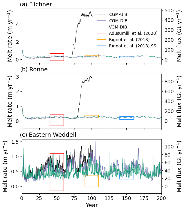
Figure 2Time series of modeled melt rates averaged over (a) Filchner Ice Shelf, (b) Ronne Ice Shelf, and (c) eastern Weddell ice shelves consisting of the Brunt, Stancomb-Wills, Riiser-Larsen, Quar, and Ekström ice shelves. The mean ± standard deviation melt rates in each region are represented by boxes placed at arbitrary years for the following: a 2003–2008 satellite-derived estimate (yellow; Rignot et al., 2013), the melt rates required to maintain the 2003–2008 steady-state ice-shelf extent (SS – blue; Rignot et al., 2013), and a 2010–2018 satellite-derived estimate (red; Adusumilli et al., 2020).
3.1 CGM-UIB
During the initial 70 years of the CGM-UIB simulation, the model reproduces the observed magnitude (Fig. 2a and b) and, to a lesser extent, the spatial distribution of Antarctic ice-shelf basal melting (Fig. 3a and b). However, after that, the total Antarctic ice-shelf melt flux nearly triples due to a large and rapid increase in melting at FRIS (Fig. 2a and b). We first evaluate these simulation results prior to reaching the FRIS melt regime change, focusing on the Weddell Sea, followed by a description of the FRIS melt regime change in Sect. 3.1.2.
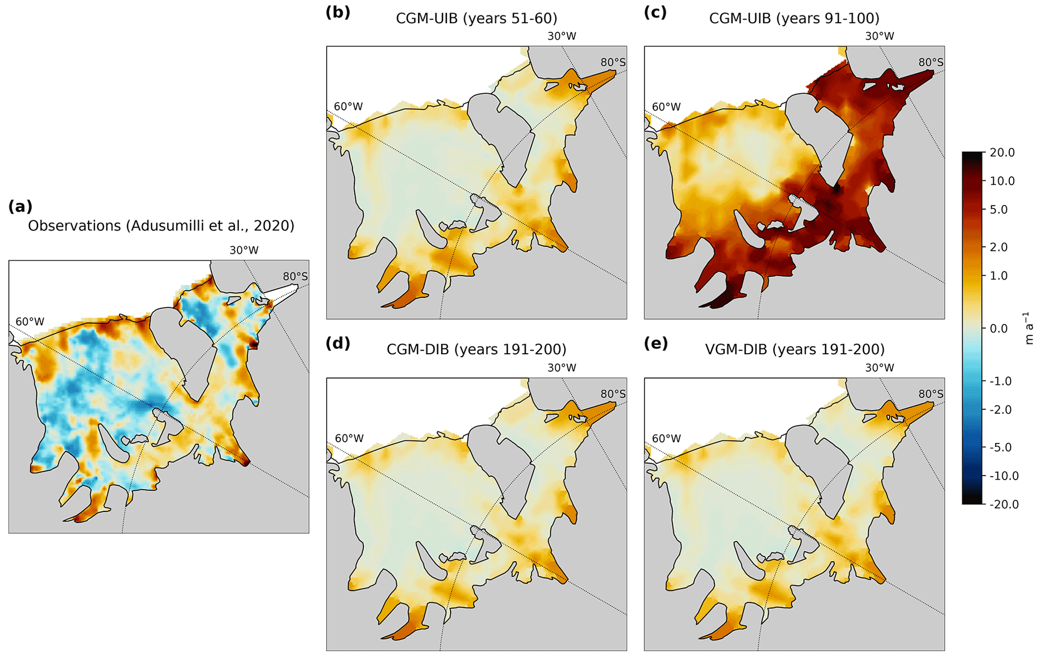
Figure 3FRIS basal melt rates (m yr−1 of freshwater). (a) Basal ice-shelf melt rate from Adusumilli et al. (2020). (b) CGM-UIB run averaged over years 51–60. (c) CGM-UIB run averaged over years 91–100 after the melt regime change has occurred. (d) CGM-DIB run averaged over years 191–200. (d) VGM-DIB run averaged over years 191–200. Note the nonlinear color scale.
3.1.1 Before FRIS melt regime change
After an initial adjustment period, the area-averaged melt rate for FRIS is within the range of observational uncertainty for both the Filchner and Ronne ice shelves (Adusumilli et al., 2020; Rignot et al., 2013; Fig. 2a and b). FRIS is large enough to be reasonably well resolved at a horizontal resolution of 35 km. However, the modeled melt rate at smaller, nearby ice shelves in the eastern Weddell Sea is too high by a factor of 4 or more (Fig. 2c). These ice shelves are poorly resolved at coarse resolution, as is the continental shelf, which is much narrower in this region relative to that of FRIS (Thoma et al., 2010).
That FRIS is adequately resolved is evidenced by a generally good match of the spatial pattern of modeled basal melting to observations (Fig. 3a and b). Similar to observations, the highest melt rates occur near the grounding lines of tributary glaciers to the ice shelf, and freezing occurs in the central portion of both the Ronne and Filchner ice shelves. However, while the area-averaged melt rate matches observations, the local magnitude of both melting and refreezing is generally smaller than observed. A notable exception to the muted spatial variability in melt flux is that the magnitude of melting near the grounding lines of tributary glaciers is generally larger than observations.
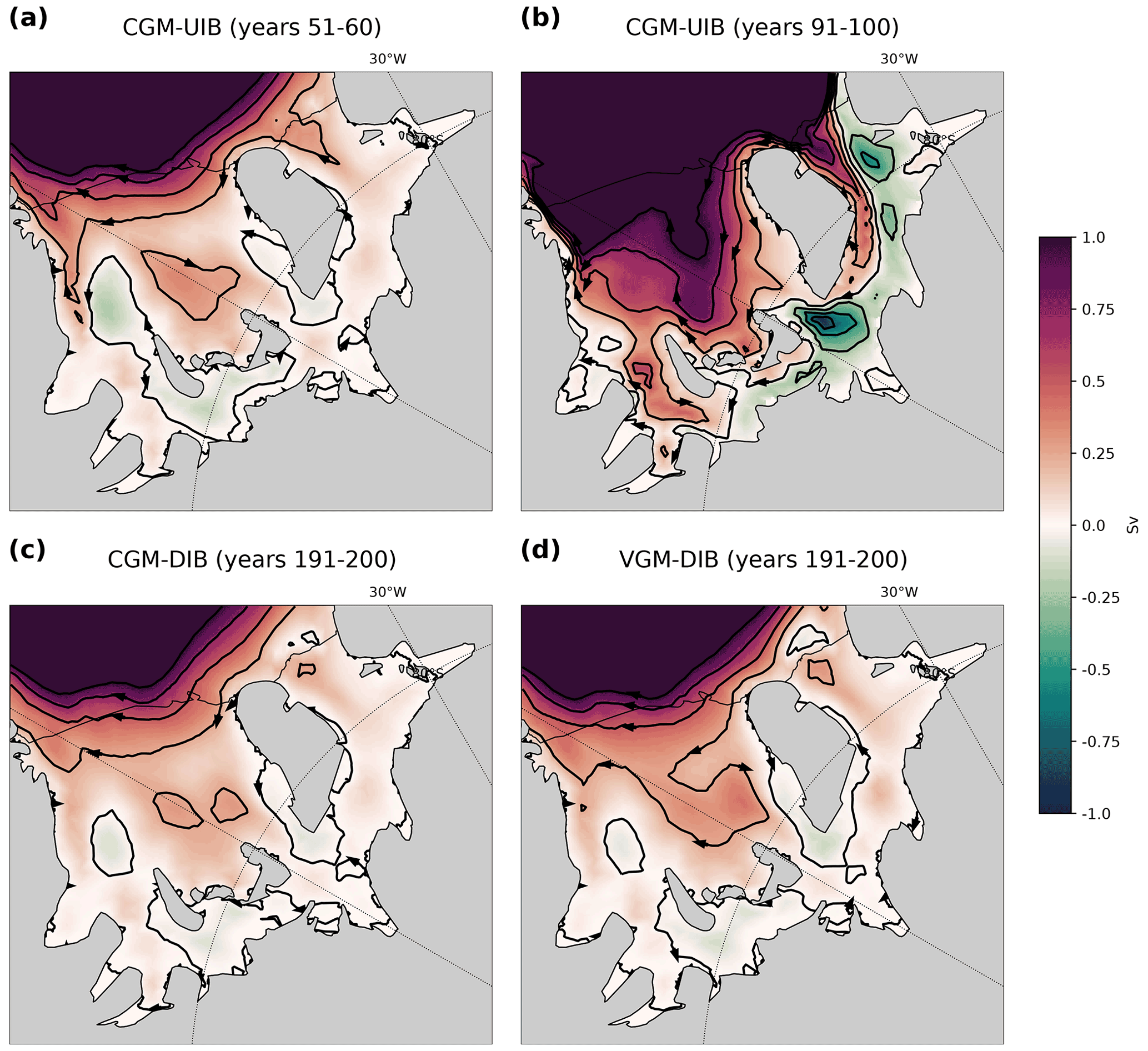
Figure 4Modeled FRIS barotropic stream function (Sv). Stream lines show the direction of depth-integrated transport, spaced at 0.25 Sv intervals. (a) CGM-UIB run averaged over years 51–60. (b) CGM-UIB run averaged over years 91–100 after the melt regime change has occurred. (c) CGM-DIB run averaged over years 191–200. (d) VGM-DIB run averaged over years 191–200.
Ocean circulation modeled beneath FRIS in the CGM-UIB simulation during the initial 70 years also follows some of the expected patterns (Nicholls et al., 2009; Hazel and Stewart, 2020; Daae et al., 2020) despite the relatively low resolution of the model (Fig. 4a). There are two primary inflow points: the Ronne Depression along the western side of the Ronne Ice Shelf and near Berkner Bank on the eastern side of Ronne Ice Shelf. A major outflow of dynamical importance for the tipping-point processes we observe is located in the Filchner Trough on the western side of the Filchner Ice Shelf, through which a combination of DSW and ice-shelf Water (ISW) flows northward. While there are no extensive observations of velocity beneath FRIS, our modeled velocities are about 5 times smaller than those produced by other models (Daae et al., 2020; Bull et al., 2021). The weaker sub-ice-shelf circulation may be partly explained by our significantly lower horizontal resolution and the absence of tides in our model. Additionally, Bull et al. (2021) showed that the strength of sub-shelf circulation is reduced as Weddell Sea continental shelf water is made fresher, a bias present in CGM-UIB.
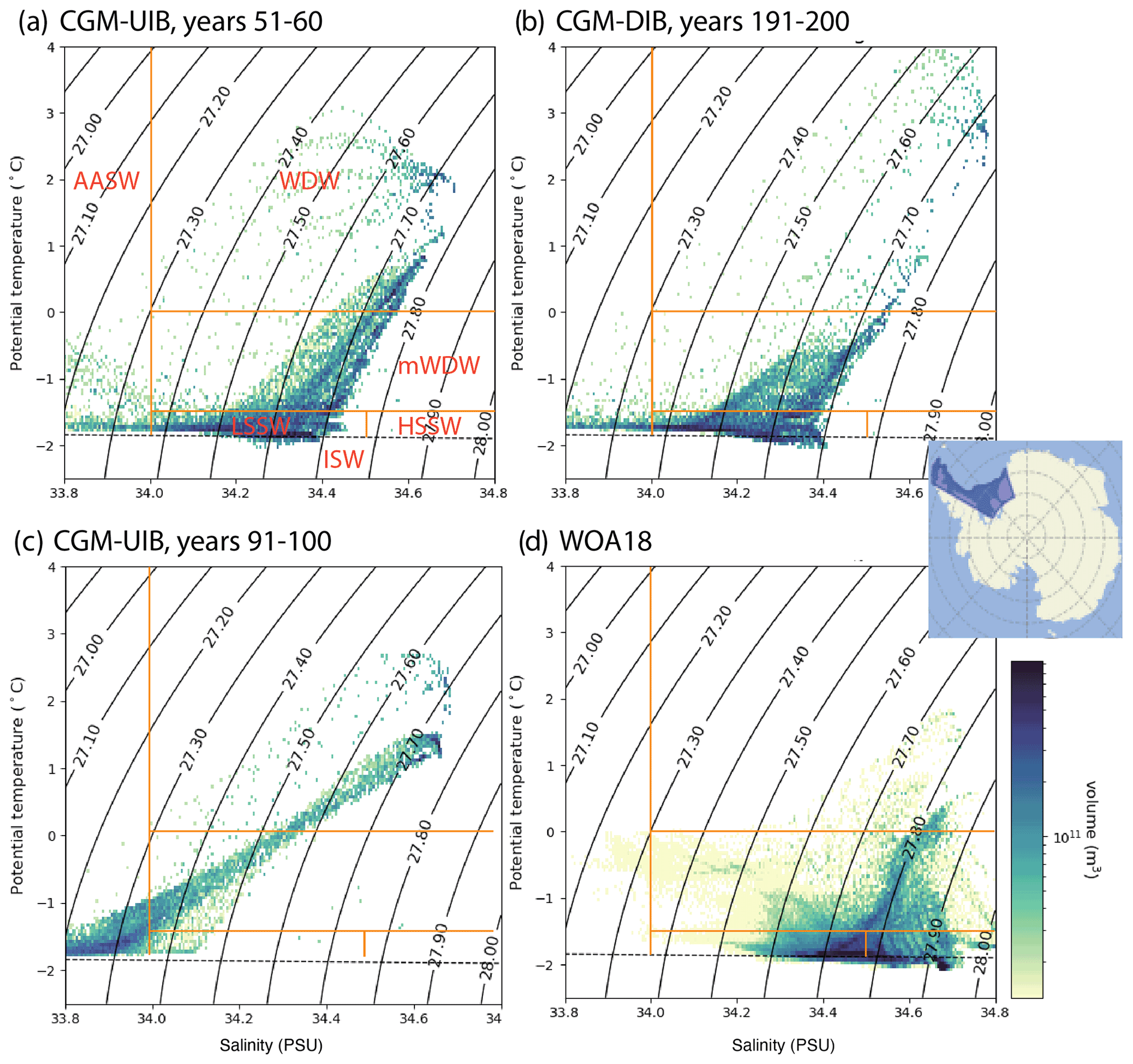
Figure 5Temperature–salinity distribution for the western Weddell Sea continental shelf for depths shallower than 1000 m. (a) CGM-UIB run averaged over years 51–60. (b) CGM-DIB run averaged over years 191–200. (c) CGM-UIB run averaged over years 91–100 after the melt regime change has occurred. (d) Observations from World Ocean Atlas, 2018. Boundaries for water masses are shown using orange lines and follow Naughten et al. (2018), renamed for Weddell Sea water masses consistent with Kerr et al. (2018): Antarctic Surface Water (AASW), Weddell Deep Water (WDW), modified Weddell Deep Water (mWDW), Low-Salinity Shelf Water (LSSW), High-Salinity Shelf Water (HSSW), and Ice-Shelf Water (ISW).
Water mass properties in the Weddell Sea in the CGM-UIB simulation have a strong fresh bias and a modest warm bias. Temperature and salinity are initialized from the Polar science center Hydrographic Climatology (PHC; Steele et al., 2001), and biases develop as the simulations progress. Fig. 5a shows temperature and salinity on the Weddell Sea continental shelf averaged over years 51–60, prior to the regime change in the control run, relative to the water mass definitions in Naughten et al. (2018) defined in Fig. 5. Using these water mass definitions, DSW is divided into Low-Salinity Shelf Water (LSSW) and High-Salinity Shelf Water (HSSW). In the CGM-UIB simulation, the primary water mass on the continental shelf is LSSW, the lighter variant of DSW. World Ocean Atlas, 2018, observations (WOA18; Locarnini et al., 2019; Zweng et al., 2019) indicate that a significant volume of HSSW is present on the continental shelf (Fig. 5d), but HSSW is effectively absent from CGM-UIB by year 20. Furthermore, the higher-density range of LSSW (> 1027.7 kg m−3) is absent from all runs by the end of the first CORE-II cycle at year 62. Thus, DSW in our simulations is characterized by LSSW rather than a combination of LSSW and HSSW. We henceforth use DSW to refer to this water mass. The second-largest water mass on the continental shelf is mWDW, but it and WDW occur in larger quantities than in the observations. ISW is present in the model in lower volume and at lower salinity than in observations.
3.1.2 FRIS melt regime change
While the present-day melt rates and circulation are represented reasonably well for the first few decades, the CGM-UIB simulation exhibits an approximately 10-fold increase in melt rate over a period of about 10 years (Fig. 2). This melt regime changes in year 71 for Filchner Ice Shelf, followed 6 years later by Ronne Ice Shelf. Once the transition to the high-melt regime occurs, melt rates remain elevated for the rest of the simulation. After the tipping point is passed, the entirety of Filchner Ice Shelf experiences highly elevated melt rates, as does the southern portion of Ronne Ice Shelf (Fig. 3c). Notably, the large-scale circulation beneath FRIS reverses after the regime change, with the strong inflow along the eastern side of Filchner Ice Shelf extending clockwise around Berkner Island (Fig. 4b). Flow beneath Ronne Ice Shelf becomes less coherent, with high velocities around the ice rises in the southern portion. These changes in circulation are consistent with those reported by higher-resolution models in the high-melt regime for FRIS (Hazel and Stewart, 2020; Daae et al., 2020).
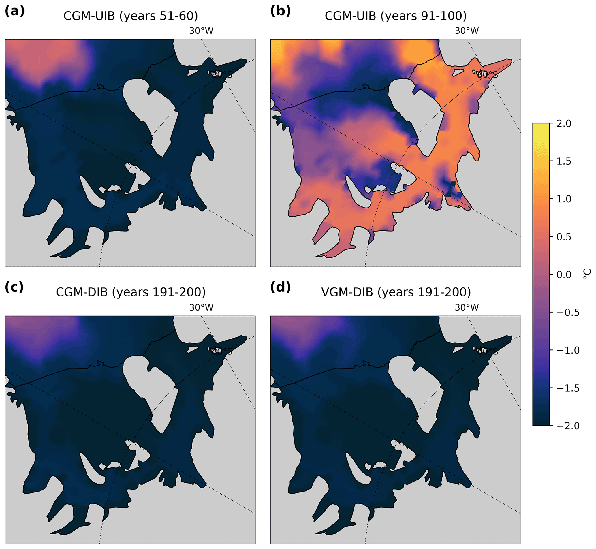
Figure 6Seafloor potential temperature. (a) CGM-UIB run averaged over years 51–60. (b) CGM-UIB run averaged over years 91–100 after the melt regime change has occurred. (c) CGM-DIB run averaged over years 191–200. (d) VGM-DIB run averaged over years 191–200.
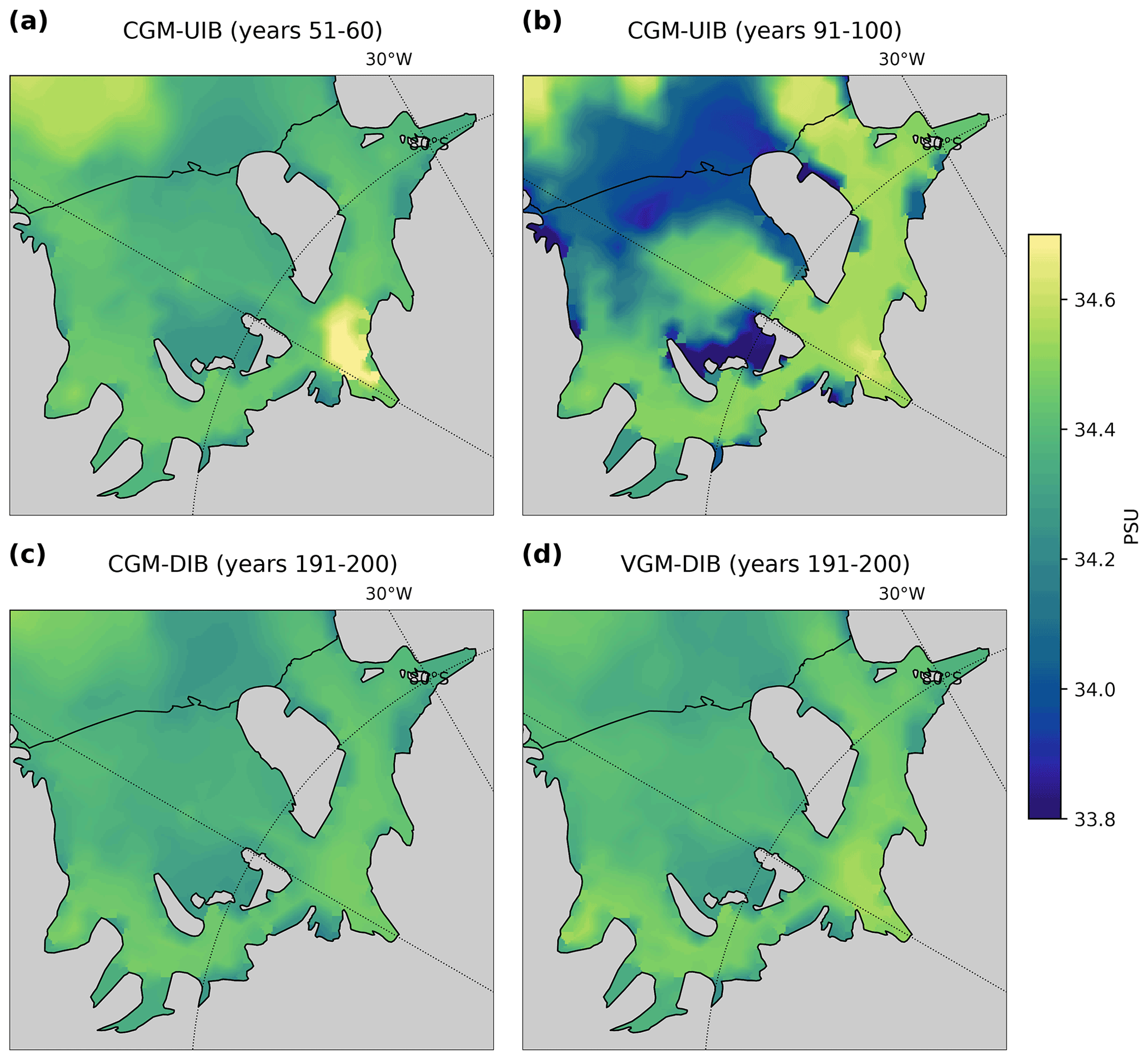
Figure 7As in Fig. 6 but showing seafloor salinity.
The FRIS melt regime change is caused by the intrusion of mWDW onto the continental shelf and beneath the Filchner Ice Shelf via the Filchner Trough, as simulated in previous modeling studies (Hellmer et al., 2012, 2017; Daae et al., 2020; Naughten et al., 2021). Prior to the melt regime change, the continental shelf seafloor is primarily occupied by cold DSW, with small incursions of mWDW from the open ocean at the Filchner Sill and the Ronne Depression (Figs. 6a and 7a). It is the Filchner Trough pathway of mWDW that leads to the melt regime change when the warm mWDW intrusion extends beyond the ice-shelf front for a sustained period. Following the intrusion, mWDW eventually fills the majority of the Filchner Ice Shelf cavity, wraps around Berkner Island, and displaces DSW throughout the majority of Ronne Ice Shelf (Figs. 6b and 7b). This can be seen in the temperature–salinity plot for after the melt regime change (Fig. 5c), where there is a clear mixing line between WDW source water mixed with AASW and an almost complete absence of DSW.
3.2 CGM-DIB
In contrast to the CGM-UIB simulation, the switch to a more realistic distribution of iceberg melting in the CGM-DIB simulation averts the FRIS melt regime change, at least through the end of the 210 years simulated (Fig. 2a and b). The FRIS basal melt distribution looks similar to the CGM-UIB simulation prior to the melt regime change and similar to observations (Fig. 3a–c). The sub-shelf circulation is also similar to the early part of the CGM-UIB run (Fig. 4a and c).
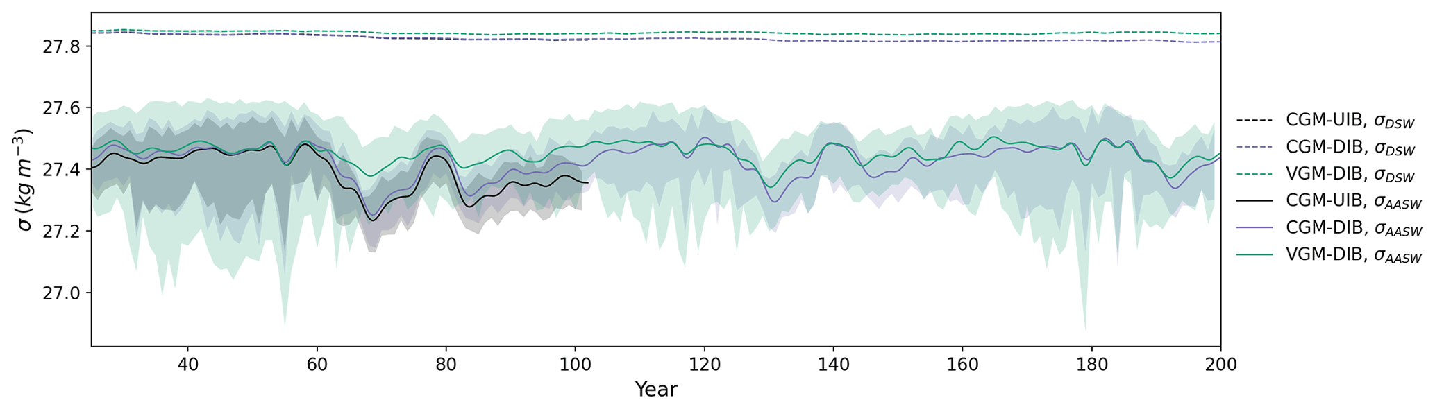
Figure 8Potential density on the Weddell Sea continental shelf between 30 and 0° W. σAASW corresponds to the average monthly density above the thermocline (solid lines), and σDSW corresponds to the average monthly density below the thermocline (dashed lines). Both quantities are low-pass-filtered in time with a cutoff of 3 months, and the running annual minimum and maximum are bounded with shading. The thermocline depth is calculated as in Hattermann (2018).
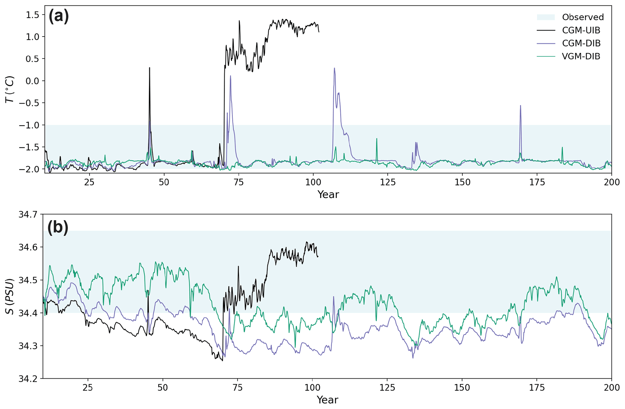
Figure 9Time series of temperature (a) and salinity (b) at observational site M31W (Ryan et al., 2017) located in the Filchner Trough (Fig. 1). The observational range is shaded.
The change in iceberg freshwater flux distribution from closer to the coast in CGM-UIB to further from the coast in CGM-DIB results in an increase in the salinity and density of DSW on the Weddell Sea continental shelf (Figs. 7 and 8). These differences are subtle at broad spatial scales (Figs. 5a–b, 7, and 8) but can be seen locally in the Filchner Trough (Fig. 9b). While the continental shelf salinity is still too low relative to observations, this water mass is sufficiently dense to limit mWDW intrusions onto the shelf. This reduction in mWDW intrusions can be seen in Fig. 9a, where mWDW intrusions only reach site M31W, ∼ 170 km from the continental shelf break (Ryan et al., 2017), once every several decades.
3.3 VGM-DIB
Although the CGM-DIB run averts the FRIS melt regime change in this historical simulation, there are several characteristics that make this simulation more prone to FRIS melt regime change than the observed system. The low continental shelf salinities lead to reduced DSW blocking of mWDW intrusions, and the high stratification in the region leads to a more baroclinic Weddell Gyre and a weaker ASF that is also more prone to mWDW intrusions. In this section, we highlight how a different treatment of eddy fluxes in the VGM-DIB simulation ameliorates these issues.
As with CGM-DIB, the VGM-DIB simulation avoids the FRIS melt regime change (Fig. 2a and b) and produces FRIS ice-shelf melt patterns that capture the major features of the observations (Fig. 3a and e). FRIS sub-shelf circulation also looks similar (Fig. 4c and d). The western Weddell Sea continental shelf temperature and salinity in the VGM-DIB run (not shown) look very similar to CGM-DIB (Fig. 5b). In addition, the periodic mWDW intrusions that reached M31W in both CGM runs are now absent (Fig. 9).
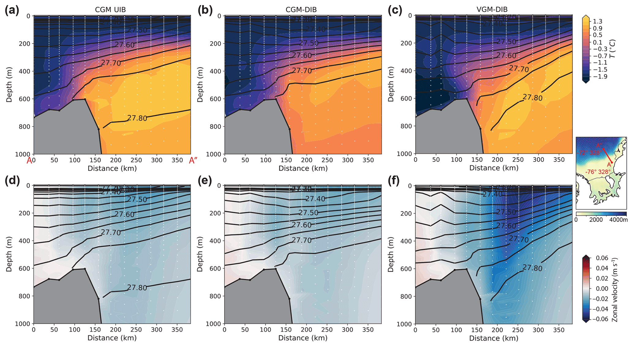
Figure 10Cross-sections across the continental shelf break at the Filchner Trough averaged over years 51 to 60 (prior to melt regime change) for CGM-UIB (a, d) and over years 191 to 200 for CGM-DIB (b, e) and VGM-DIB (c, f). Panels (a–c) show temperature (colors) and potential density anomalies (contours, referenced to the surface). Panels (d–f) show eastward zonal velocity (colors) with potential density anomalies as in (a–c). White dots indicate model data points used to construct the cross-section. The inset map shows the location of transect A-A′′, as does Fig. 1.
The ASF plays a critical role in modulating transport of heat onto the Weddell continental shelf. Our simulations consistently feature weaker ASF characteristics than observations, making them more prone to mWDW intrusions. We characterize the ASF based on the thermocline depression from off-shelf to on-shelf; all our simulations show much smaller thermocline depressions than observed: roughly 200 m rather than 450 m (Hattermann, 2018). However, there is a notable improvement in the strength of the ASF in the VGM-DIB simulation (Fig. 10b and c), as seen in more steeply sloping isopycnals at the continental shelf break and the greater difference in depth of the thermocline between the shelf break and open ocean. The presence of a thinner warm layer at the seafloor along the Filchner Trough in VGM-DIB relative to CGM-DIB (Fig. 10b and c) demonstrates the decreased access of offshore mWDW to the continental shelf.
The use of a spatially varying bolus parameter in this run appears to have reduced cross-ASF heat transport and maintained a steeper ASF.
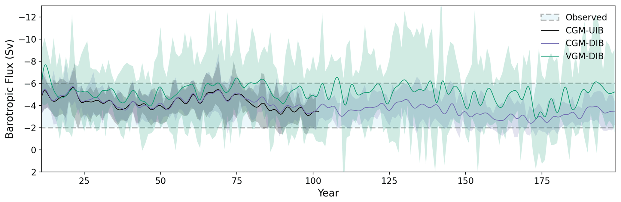
Figure 11Simulated barotropic transport associated with the Antarctic Slope Current and the southern branch of the Weddell Gyre near the Filchner Trough (Fig. 1; A′-A′′). The southern end of the transect (A′) is the 750 m bathymetric contour. The barotropic flux is computed from monthly averaged eastward zonal velocities and low-pass filtered in time with a cutoff of 3 months, and the running annual minimum and maximum are bounded with shading. Simulated barotropic transport with a higher-resolution ocean model forced by atmospheric climatology (Wang et al., 2012, their Fig. 1) is shown using dashed lines and blue shading.
The other factor responsible for a more robust ASF in the VGM-DIB run is the reduction in salinity biases, which improves the density structure on the continental shelf and at the shelf break. The fresh bias in the CGM-UIB and CGM-DIB simulations is also associated with excessive near-surface stratification in the Weddell Gyre (Fig. 10a and b). The result of this stratification is a more baroclinic Weddell Gyre, as less momentum from wind stress is transferred below the surface layer. Partially ameliorating these biases in the VGM-DIB run led to slightly less stratification (Fig. 10c) and a more barotropic Weddell Gyre (Fig. 11). The Weddell Gyre's barotropic transport near the Filchner Trough in our simulations is within the 2–6 Sv range given by higher-resolution regional models with similar forcing (Wang et al., 2012, Fig. 11). Barotropic transport in the Weddell Gyre is dynamically associated with a larger ASF thermocline depression through Ekman downwelling, which is consistent with our simulations (Hattermann, 2018).
Thus, the modified eddy representation in VGM-DIB affects mWDW transport both directly through eddy fluxes across the ASF and indirectly through water mass changes. The relative importance of these direct and indirect effects is not possible to disentangle using our experimental design and existing model diagnostics. Regardless, the VGM-DIB simulation represents the most realistic configuration of E3SM's ocean and sea-ice components at this resolution for the Weddell Sea and FRIS.
3.4 Prescribed melt branch runs
As expected, the prescribed melt branch runs with mean baseline melt fluxes for the eastern Weddell Sea-ice shelves do not experience the FRIS regime change (Fig. 12a and b). However, modestly elevated melt rates applied to the eastern Weddell Sea ice shelves trigger the FRIS melt regime change. For CGM-DIB, all experiments with an eastern Weddell Sea melt rate of 2 m yr−1 and higher lead to the FRIS regime change, whereas for VGM-DIB, the FRIS regime change occurs with eastern Weddell Sea melt rates of 4 m yr−1 and higher. As seen in the CGM-UIB baseline run, in all runs exhibiting the melt regime change, Filchner Ice Shelf transitions to a high-melt regime first, followed by Ronne Ice Shelf within a decade. While the lowest melt rates applied do not lead to the occurrence of the FRIS melt regime change, all branch runs were stopped after 62 years (a complete CORE-II forcing cycle), and we are not able to rule out the possibility of these leading to a FRIS melt regime change later. All simulations that lead to the FRIS regime change begin that transition within 21 years of the imposed eastern Weddell Sea melt rates. Increasing the melt rate applied reduces the time until the FRIS melt regime change occurs (Fig. 12c). This effect is sensitive to model baseline state, with CGM-DIB reaching the tipping point more quickly and at lower prescribed melt rates than VGM-DIB, consistent with the behavior in the previous simulations with fully prognostic ice-shelf melt fluxes.
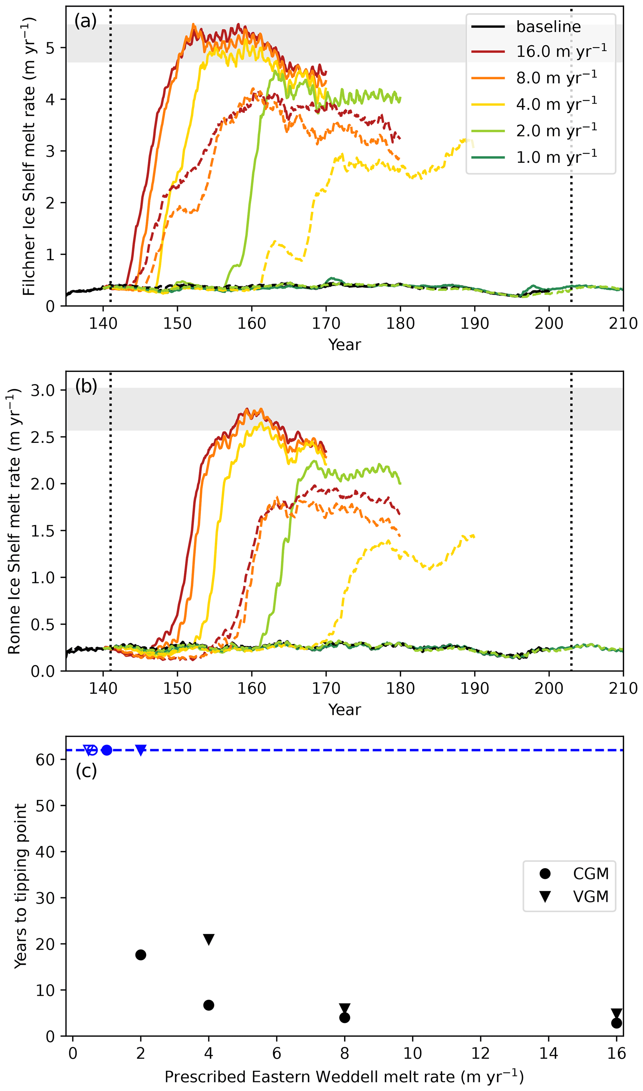
Figure 12Results of branch runs prescribing melt rates at eastern Weddell Sea ice shelves. All branch runs were begun in year 141 and stopped after 62 years (one complete CORE-II cycle), indicated by dotted vertical lines. (a) Area-averaged melt rate modeled at Filchner Ice Shelf. CGM-DIB is shown with solid lines, and VGM-DIB is shown with dashed lines. The baseline simulations are shown in black. The gray shading indicates the range of melt rates simulated after the regime change in the CGM-UIB run. (b) Area-averaged melt rate modeled at Ronne Ice Shelf. The line styles are the same as for panel (a). (c) Number of years to occurrence of the FRIS tipping point as a function of the melt rate prescribed at the eastern Weddell Sea ice shelves for both CGM-DIB (circles) and VGM-DIB (triangles). The open symbols represent the baseline runs. The initiation of the FRIS tipping point is defined here as the first year in which the modeled Filchner Ice Shelf melt rate exceeds twice the mean baseline value. The blue symbols on the dashed blue line indicate simulations that did not reach the FRIS tipping point within a complete CORE-II forcing cycle.
The simulations that are slower to initiate transition to the elevated FRIS melt regime experience a longer transition period (Fig. 12a and b). They also exhibit a non-monotonic increase in Filchner Ice Shelf melt rate during the transition (Fig. 12a). These temporary increases in Filchner Ice Shelf melt rate appear to be from pulses of mWDW intrusion (similar to those shown in Fig. 9) driven by surface forcing from which melt rates partially recover before the next surface forcing event occurs. For the simulations experiencing a rapid transition to high Filchner Ice Shelf melt rates, the reorganization of the sub-shelf circulation is reinforced too quickly for these variations in surface-driven mWDW intrusion to be exhibited.
Notably, the magnitude of FRIS melt rates after the regime change is a function of both the applied melt perturbations in the eastern Weddell Sea and the eddy parameterization (Fig. 12a and b). Higher imposed melt rates in the eastern Weddell Sea lead to larger post-transition FRIS melt rates. The CGM-DIB configurations yield higher post-transition FRIS melt rates than VGM-DIB for both Filchner and Ronne ice shelves.
4.1 Mechanisms for FRIS melt regime change
The fact that the CGM-UIB simulation undergoes a FRIS melt regime change under historical forcing is clearly inconsistent with historically observed low FRIS melt rates. Of the possible explanations for this inconsistency, two plausible candidates are that (1) the simulated state is closer to the FRIS tipping point than the historical state and that (2) the model's process representations shift the tipping point in state space relative to the real-world tipping point. We discuss these two candidates in the context of our suite of simulations, which feature both changes in the simulated state and changes in the model representation of eddy processes. First, we show that our simulated state in CGM-UIB is consistent with the two ocean conditions for the FRIS regime change identified by Daae et al. (2020), using systematic perturbations to a high-resolution coupled ocean and sea-ice model. Then we examine each condition in relation to changes in model representations across our simulation suite: the switch from spatially uniform to variable iceberg fluxes and from a constant to a variable GM eddy parameter.
Daae et al. (2020) demonstrated in their modeling study that both low continental shelf salinity and thermocline shoaling at the continental shelf break were necessary for a FRIS regime shift. The CGM-UIB simulation meets both of these criteria for FRIS regime shift (Figs. 5a and c and 10a) and manifests that regime shift. The Weddell Shelf salinities in CGM-UIB are much lower than observed (Fig. 5a), consistent with the “strong freshening” scenario of Daae et al. (2020) in which DSW salinities are less than 34.4 PSU (the maximum salinity of DSW in CGM-UIB is 34.3 PSU). The CGM-UIB simulation also has a thermocline that is between 200 and 300 m shallower than observed (not shown). In the simulations of Daae et al. (2020), thermocline shoaling of 200 m was sufficient to cause the FRIS regime shift. Thus, the lower-resolution CGM-UIB simulation is at least as sensitive to the FRIS melt regime change as the higher-resolution simulations of Daae et al. (2020).
The DSW salinity bias in our simulations is likely due to a combination of factors. One factor examined in Comeau et al. (2022) is the representation of mesoscale eddy fluxes; the VGM representation of mesoscale eddy fluxes results in much higher continental shelf salinities. In CGM-UIB, there is an additional contribution to DSW freshening by preferential iceberg fluxes near the coast. These iceberg fluxes freshen the surface more than at depth, enhancing the stratification between AASW and DSW (Fig. 10a; e.g., depth of the 27.50 kg m−3 potential density anomaly contour). This stratification further contributes to DSW freshening because it inhibits the wintertime convection that would normally restore DSW salinities. Similarly, the addition of ice-shelf melt fluxes has been shown to increase stratification in E3SM and exacerbate DSW salinity biases on the Weddell continental shelf (Jeong et al., 2020).
The change in iceberg flux distribution between CGM-UIB and CGM-DIB has small effects on continental shelf density, namely, the increase in density above the thermocline due to the change in iceberg distribution is less than 0.1 kg m−3 (Figs. 8 and 10a, b) but is sufficient to avert the regime shift. This suggests either a high sensitivity to DSW density or a sensitivity to cross-slope gradients in buoyancy fluxes. An increase in the gradient of buoyancy fluxes (decreasing from onshore to offshore) may weaken the ASF through enhanced baroclinic eddy formation associated with the frontal instability (Marshall and Radko, 2003). This process tends to flatten the ASF isopycnals and would reduce the barrier to mWDW intrusions. This buoyancy flux gradient effect is hypothesized to have contributed to a temporary increase in mWDW intrusion strength after a significant sea-ice melting event on the eastern Weddell continental shelf (Ryan et al., 2020). However, we did not find evidence for a significantly different ASF isopycnal slope between CGM-UIB and CGM-DIB (Fig. 10a and b), suggesting that these baroclinic eddy fluxes, parameterized in our model, were not significantly different. Thus, we hypothesize that the FRIS regime shift in our simulations displays a high sensitivity to DSW salinities. The branch runs with different eastern Weddell melt rates also correspond to different diffuse DSW salinity perturbations, in contrast to perturbations of the local buoyancy gradient. That these branch runs resulted in different timings of FRIS regime change also lends support to the hypothesis that DSW salinity is the more important regime change factor in our simulations. Thus, our study corroborates Timmermann and Hellmer (2013) and Daae et al. (2020) in finding that continental shelf salinity is a major control on mWDW inflow.
The thermocline shoaling in our simulations is a consequence of modeled water mass biases in the region. The density contrast between AASW and WDW is thought to exert a strong control on the thermocline depression (Hattermann, 2018). As this density stratification increases, the Antarctic Slope Current (ASC) flow becomes more baroclinic, and the thermocline depression decreases (Hattermann, 2018; Daae et al., 2020). While the thermocline depression is lower than the observations in all of our simulations (Fig. 10), the VGM parameterization of mesoscale eddy fluxes is sufficient to strengthen the Weddell Gyre and provide a dynamical barrier to WDW intrusions. Thus, VGM-DIB demonstrates how both a more realistic iceberg flux distribution and a modification to the mesoscale eddy parameterization in coarse-resolution ocean models can prevent the regime shift at FRIS despite persistent water mass biases. Our results highlight the relevance of a two-pronged approach to improving the realism of FRIS regime change by improving both ocean model state biases and process representation. In Sect. 4.3, we further discuss the prospects for accurate simulation of the FRIS regime change by climate models. In summary, we conclude that the propensity of this model configuration to FRIS melt regime change is primarily due to biases in the simulated state as opposed to a shift in the tipping point in the model relative to the real world; we find that our simulations trigger the melt regime change under similar physical conditions to other models but that our model is more prone to the change because its biases place it unrealistically close to the tipping point.
4.2 Remote influence between ice-shelf melt fluxes in the model
Our model results provide clear evidence for the potential of remote influence between ice-shelf basal melt fluxes through the advection of meltwater and its impact on continental shelf salinity and density. While this is the first study to our knowledge to explicitly link the melt fluxes between different ice shelves, this work builds on previous studies linking ice-shelf meltwater fluxes to distant ocean conditions and vice versa. In a high-resolution ocean model, Nakayama et al. (2014) linked increasing ice-shelf melt in the Amundsen Sea to freshening in the Ross Sea via advection by the ASC, and Nakayama et al. (2020) identified that the freshening could extend to the Weddell Sea under large Amundsen Sea melt rates. The timescale of transport between adjacent regions is a few years in our simulations, consistent with other higher-resolution simulations (Dawson et al., 2023) and with the rapid initiation of FRIS melt regime change in our eastern Weddell Sea prescribed melt branch runs (Fig. 12). Nakayama et al. (2020) suggest that transport of freshwater anomalies is enhanced by strengthening of the ASC as density gradients across the ASF increase, an effect not investigated here and unlikely to be resolved well in our low-resolution simulations.
Imposing freshwater fluxes representing Antarctic ice-shelf melt and similar “hosing” experiments have been conducted in a number of global climate models that did not include prognostic ice-shelf basal melt fluxes (e.g., Fogwill et al., 2015; Phipps et al., 2016; Pauling et al., 2016, 2017; Bronselaer et al., 2018; Moorman et al., 2020). While these studies generally agree that increased freshwater fluxes on the continental shelf lead to increased ocean stratification, the net effect on cross-shelf heat fluxes is nuanced. In low-resolution models, this stratification leads to increased warming at depth and an implied positive feedback in ice-shelf basal melting (Fogwill et al., 2015; Phipps et al., 2016; Bronselaer et al., 2018). In high-resolution (eddy-permitting) models, freshening on the continental shelf may weaken cross-shelf heat fluxes by strengthening density gradients across the ASF (Moorman et al., 2020) or enhance cross-shelf heat fluxes through baroclinic instability in the ASF and through tidal mixing (Si et al., 2023). It is worth noting that the change in heat flux into the FRIS cavity may in fact be minor with a small degree of freshening (𝒪(0.01) PSU) in the eastern Weddell ASC, as revealed by further regional eddy-permitting simulations (Bull et al., 2021). Thus, more work remains to reconcile the potential effects of freshwater fluxes and their spatial distributions on FRIS regime change across the modeling studies that have been conducted thus far, particularly for larger freshwater perturbations such as those explored here.
4.3 Challenges of representing Antarctic ice shelves in climate models
We have demonstrated the potential for a FRIS melt regime change in a CMIP-class ocean–sea-ice model due to biases in salinity and ASC strength in the Weddell Sea. While our model biases are larger than in many regional ocean modeling studies, global ocean models used in Earth system models do not have the benefit of regional lateral boundary conditions to constrain model behavior in the Weddell Sea. Given what we understand about the FRIS melt regime change, here we place the E3SM results from our global ocean–sea-ice configuration in context and comment on the applicability of CMIP models in this region.
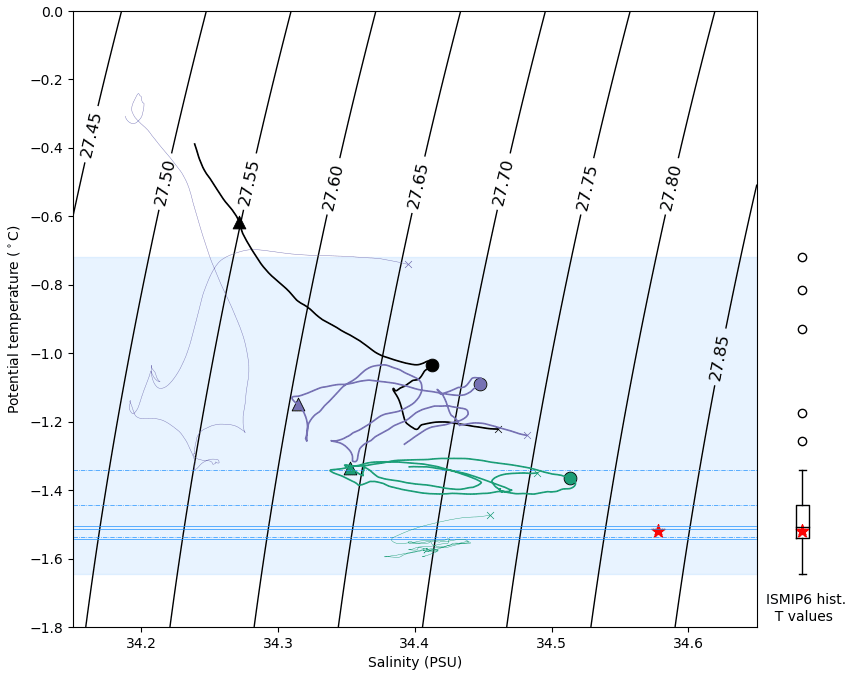
Figure 13Comparison of modeled Weddell Sea continental shelf water mass properties in the E3SM and CMIP5 models used in the ISMIP6 intercomparison. Observed temperature and salinity from WOA are indicated by the red star. The modeled temperature and salinity are represented by their 20-year-mean trajectories, with the initial 20-year average indicated by an x. The three primary global ocean–sea-ice simulations described in this paper are shown with thick lines and colored symbols (CGM-UIB – black; CGM-DIB – purple; and VGM-DIB – green). Circles mark the average over years 42–62 (the final 20 years before the end of the first CORE-II cycle), and triangles are for the average over years 70–90 (the final 2 complete decades before CGM-UIB begins regime shift). The equivalent fully coupled E3SM preindustrial spin-ups from Comeau et al. (2022) are indicated by thin lines in corresponding colors (coupled CGM-DIB – purple and coupled VGM-DIB – green) covering 200 years. The temperature range from the ensemble of CMIP5 historical simulations evaluated by Barthel et al. (2020) is indicated by the blue shading and also represented in more detail by the box and whisker plot on the right-hand side (with outliers as circles). The CMIP5 models selected for ISMIP6 are added for context (top 3 – blue lines and top 6 – dashed blue lines).
Barthel et al. (2020) evaluated ocean temperatures from 33 climate models in 6 Antarctic continental shelf regions against a 1979–2005 historical climatology of coastal water masses compiled from shipboard measurements, instrumented seals, and reanalysis to select climate model forcing for the Ice Sheet Model Intercomparison Project for CMIP6 (ISMIP6). E3SM was not complete for CMIP5, so we show E3SM results in context of the CMIP5 models in Fig. 13. While the analysis shown by Barthel et al. (2020) only evaluated temperature, for E3SM simulations in Fig. 13 we show the 20-year rolling mean trajectory in temperature–salinity (T,S) space. In addition to the ocean and sea-ice configuration described in this study, we show the fully coupled (atmosphere–land–river–ocean–sea-ice) E3SM simulations described by Comeau et al. (2022). Note that because E3SM v1.2 was not applied to historical simulations, the fully coupled E3SM results shown in Fig. 13 represent constant preindustrial climate conditions, while the analysis of Barthel et al. (2020) considered the 1979–2005 historical period – the comparison is intended to be illustrative.
Overall, the E3SM simulations tend to be biased fresh and warm compared to observations. The fully coupled Constant Gent–McWilliams (CGM) simulation described by Comeau et al. (2022, thin purple line) exhibits an early drift to fresher biases. Over the course of its 160 years of simulation (by which time it exhibits a regime shift), it would be amongst the outliers in the CMIP5 ensemble (beyond the 1.5 interquartile range from the mean, shown by the empty circles) with a temperature bias in this region that ranges from 0.8° over years 10–30, making it the worst of the CMIP5 ensemble, to 0.2° over years 79–99, exceeded by the five CMIP5 outliers. In contrast, the fully coupled VGM simulation (green; see Comeau et al., 2022) remains stable in (T,S) space and within the temperature range covered by the CMIP5 models used for ISMIP6.
Of the global ocean–sea-ice historical simulations described in this study, the trajectory of CGM-UIB (thick black line) towards the FRIS melt regime change can be seen by its rapid evolution to fresher, warmer conditions in the Weddell Sea, similar to the fully coupled CGM simulation (thin black line). The CGM-DIB simulation avoids the regime change but still exhibits a warm bias and freshening over the course of the simulation. Our favored configuration, VGM-DIB, also freshens over the simulation but exhibits the smallest salinity and temperature biases. Overall, we note that despite its biases, the global ocean–sea-ice configuration of E3SM is not outside of the CMIP5 range, as it exhibits temperature biases ranging from middle-of-the-road CMIP models to the warmer CMIP5 outliers depending on its parameterization. Issues such as a FRIS melt regime shift may be encountered by other models, particularly once they account for freshwater from ice-shelf melt or icebergs.
While it is not possible to identify an absolute threshold in regional salinity that avoids a FRIS melt regime shift for all models (Hellmer et al., 2017; Daae et al., 2020; Haid et al., 2023), this comparison for E3SM configurations with and without regime change provides some guidance for climate model evaluation in this region. As recent studies have clearly identified the importance of continental shelf salinity for controlling FRIS melt regime through its impact on density (Daae et al., 2020; Bull et al., 2021; Haid et al., 2023), we recommend that future evaluations of ocean models for forcing ice-sheet models consider regional salinity in addition to temperature.
Our results demonstrate that while the inclusion of ice-shelf cavities and prognostic ice-shelf basal melt rates are critical for projecting changes in the Antarctic, the significant technical challenges of introducing these capabilities to Earth system models are compounded by potential complications from regional model biases that may be difficult to improve in a global climate model. While typical standalone parameterizations of ice-shelf basal melt (e.g., Jourdain et al., 2020) forced by offshore ocean conditions would not produce a melt regime change even with a regional fresh bias, the same ocean conditions can lead to melt regime change and rapid changes to continental shelf temperature and salinity with prognostic melt fluxes in an ocean model. To date, the other CMIP-class ocean model with prognostic ice-shelf melt fluxes also exhibits a fresh bias in the Weddell Sea (and Ross Sea), which leads to FRIS melt regime change in SSP5-8.5 projections around 2100 (Siahaan et al., 2022). Typical features of CMIP-class ocean models, such as modest resolution requiring parameterization of mesoscale eddies, under-resolved coastal polynyas, use of vertical mixing schemes not developed for polar conditions, simplified treatment of iceberg freshwater fluxes, and a lack of tides, contribute to challenges in resolving the key processes of DSW formation and ASF dynamics. Process studies and high-resolution modeling will remain critical for guiding improvement of low-resolution global ocean models applied in the Antarctic.
We have investigated the occurrence of a FRIS basal melt regime change in low-resolution E3SM v1.2 global ocean–sea-ice simulations forced by historical atmospheric reanalysis. As seen in the fully coupled E3SM (Comeau et al., 2022), careful treatment of iceberg melt fluxes and the mesoscale eddy parameterization is necessary to achieve realistic simulations of this region that avoid a FRIS melt regime change. While moving the iceberg melt flux from uniform around the Antarctic coast to a realistic spatial distribution avoids the tipping point, switching to a spatially variable bolus coefficient in the Gent–McWilliams parameterization further improves continental shelf salinity, ASF structure, and barotropic transport in the region, despite lingering fresh surface biases leading to an overly stratified ocean and excess heat at depth. With these features, E3SM is able to produce the broad-scale patterns of present-day FRIS melt rates and cavity circulation even at relatively low horizontal ocean resolution.
To investigate the sensitivity of FRIS to freshwater fluxes in the region, we conducted a series of perturbation experiments where the ice shelves in the eastern Weddell Sea were given increasingly larger prescribed melt rates. We find that melt rates of 2–4 m yr−1 are sufficient to trigger the FRIS melt regime change in our global ocean–sea-ice configurations and that the regime change initiates sooner at higher upstream melt rates. This work explicitly identified the possibility of remote connections between Antarctic ice-shelf basal melt fluxes, building on previous work linking freshwater fluxes and ice-shelf melt rates around Antarctica. Because of the interplay between ice-shelf basal melt fluxes and ocean conditions that we find here, we caution against inferring ice-shelf melt rates from modeled ocean state without prognostic melt fluxes.
Finally, we put E3SM regional biases in the context of other climate models that have been evaluated in the region and find that E3SM skill in this region is comparable to other CMIP models and that the improvements discussed in this paper improve model skill. We discuss challenges in adding prognostic basal melt fluxes to global climate models and highlight their importance in reproducing continental shelf salinity and ASF strength for simulating ice-shelf melting. Challenges remain in projecting ice-shelf melting in climate models due to their low resolution and lack of some key processes. Continuing to integrate knowledge gained from observations and process models is critical for projecting the state of the Southern Ocean under future climate scenarios and under the associated impacts on the Antarctic ice sheet and sea-level change.
The E3SM code is available at https://github.com/E3SM-Project/E3SM (last access: 9 March 2024), and the model version used for the simulations presented here is E3SM v1.2.1 (https://doi.org/10.11578/E3SM/dc.20210309.1; E3SM Project, 2020). Information about running the model is available at https://e3sm.org/model/running-e3sm (E3SM, 2024). Simulation data used for this paper are available on the ESGF website at https://aims2.llnl.gov/search/E3SM?project=E3SM&activeFacets =7B22campaign223A22Cryosphere-v1222C22experiment223A22G-IAF-DIB-ISMF227D (Comeau, 2021a) and https://aims2.llnl.gov/search/E3SM?project=E3SM&activeFacets =7B22campaign223A22Cryosphere-v1222C22experiment223A22G-IAF-DIB-ISMF-3dGM227D (Comeau, 2021b). The CGM-UIB run and prescribed melt branch runs are available upon request. Most of the analysis on the ocean component MPAS-Ocean was performed using MPAS-Analysis, available at https://github.com/MPAS-Dev/MPAS-Analysis (https://doi.org/10.5281/zenodo.5109439; Asay-Davis et al., 2021).
MJH conceptualized the research, and MJH, CBB, and XSAD developed the simulation plan methodology. DC, XSAD, JW, and MJH developed the software configuration of E3SM used in these simulations. DC and MJH conducted the simulations described here. CBB, MJH, XSAD, DC, and AB analyzed and visualized the simulation results. MJH and CB prepared the original manuscript draft, and all authors contributed to the review and editing process. SFP also contributed funding and acquired resources.
The contact author has declared that none of the authors has any competing interests.
Publisher's note: Copernicus Publications remains neutral with regard to jurisdictional claims made in the text, published maps, institutional affiliations, or any other geographical representation in this paper. While Copernicus Publications makes every effort to include appropriate place names, the final responsibility lies with the authors.
This work was supported by the Biological and Environmental Research program, funded by the US Department of Energy (DOE) Office of Science. This work was also supported by the DOE Office of Science Early Career Research program. This research used a high-performance-computing cluster provided by the BER Earth System Modeling program and operated by the Laboratory Computing Resource Center at Argonne National Laboratory. This research used resources of the National Energy Research Scientific Computing Center, a DOE Office of Science User Facility supported by the Office of Science of the US Department of Energy under contract no. DE-AC02-05CH11231. We acknowledge the Norwegian Polar Institute's Quantarctica package.
This research has been supported by the DOE Office of Science Biological and Environmental Research program, the DOE Office of Science National Energy Research Scientific Computing Center (grant no. DE-AC02-05CH11231), and the DOE Office of Science Advanced Scientific Computing Research program.
This paper was edited by Alexander Robinson and reviewed by two anonymous referees.
Adcroft, A. and Campin, J.-M.: Rescaled height coordinates for accurate representation of free-surface flows in ocean circulation models, Ocean Model., 7, 269–284, https://doi.org/10.1016/j.ocemod.2003.09.003, 2004. a
Adusumilli, S., Fricker, H. A., Medley, B., Padman, L., and Siegfried, M. R.: Interannual variations in meltwater input to the Southern Ocean from Antarctic ice shelves, Nat. Geosci., 13, 616–620, https://doi.org/10.1038/s41561-020-0616-z, 2020. a, b, c, d
Asay-Davis, X.: MPAS-Dev/MPAS-Analysis: v1.4.0 (1.4.0), Zenodo [code], https://doi.org/10.5281/zenodo.5109439, 2021. a
Barthel, A., Agosta, C., Little, C. M., Hattermann, T., Jourdain, N. C., Goelzer, H., Nowicki, S., Seroussi, H., Straneo, F., and Bracegirdle, T. J.: CMIP5 model selection for ISMIP6 ice sheet model forcing: Greenland and Antarctica, The Cryosphere, 14, 855–879, https://doi.org/10.5194/tc-14-855-2020, 2020. a, b, c, d
Bisht, G., Riley, W. J., Hammond, G. E., and Lorenzetti, D. M.: Development and evaluation of a variably saturated flow model in the global E3SM Land Model (ELM) version 1.0, Geosci. Model Dev., 11, 4085–4102, https://doi.org/10.5194/gmd-11-4085-2018, 2018. a
Bronselaer, B., Winton, M., Griffies, S. M., Hurlin, W. J., Rodgers, K. B., Sergienko, O. V., Stouffer, R. J., and Russell, J. L.: Change in future climate due to Antarctic meltwater, Nature, 564, 53–58, https://doi.org/10.1038/s41586-018-0712-z, 2018. a, b
Bull, C. Y. S., Jenkins, A., Jourdain, N. C., Vǎková, I., Holland, P. R., Mathiot, P., Hausmann, U., and Sallée, J.: Remote Control of Filchner-Ronne Ice Shelf Melt Rates by the Antarctic Slope Current, J. Geophys. Res.-Oceans, 126, e2020JC016550, https://doi.org/10.1029/2020JC016550, 2021. a, b, c, d, e
Burrows, S. M., Maltrud, M., Yang, X., Zhu, Q., Jeffery, N., Shi, X., Ricciuto, D., Wang, S., Bisht, G., Tang, J., Wolfe, J., Harrop, B. E., Singh, B., Brent, L., Baldwin, S., Zhou, T., Cameron-Smith, P., Keen, N., Collier, N., Xu, M., Hunke, E. C., Elliott, S. M., Turner, A. K., Li, H., Wang, H., Golaz, J. C., Bond-Lamberty, B., Hoffman, F. M., Riley, W. J., Thornton, P. E., Calvin, K., and Leung, L. R.: The DOE E3SM v1.1 Biogeochemistry Configuration: Description and Simulated Ecosystem-Climate Responses to Historical Changes in Forcing, J. Adv. Model. Earth Sy., 12, 1–59, https://doi.org/10.1029/2019MS001766, 2020. a
Church, J., Clark, P., Cazenave, A., Gregory, J., Jevrejeva, S., Levermann, A., Merrifield, M., Milne, G., Nerem, R., Nunn, P., Payne, A., Pfeffer, W., Stammer, D., and Unnikrishnan, A.: Sea Level Change, in: Climate Change 2013: The Physical Science Basis. Contribution of Working Group I to the Fifth Assessment Report of the Intergovernmental Panel on Climate Change, edited by: Stocker, T., Qin, D., Plattner, G.-K., Tignor, M., Allen, S., Boschung, J., Nauels, A., Xia, Y., Bex, V., and Midgley, P., Cambridge University Press, Cambridge, United Kingdom and New York, NY, USA, pp. 1137–1216, 2013. a
Comeau, D.: CGM-DIB simulation data, Earth System Grid Federation [data set], https://aims2.llnl.gov/search/E3SM?project=E3SM&activeFacets =% 7B% 22campaign% 22% 3A% 22Cryosphere-v1% 22% 2C% 22experiment% 22% 3A% 22G-IAF-DIB-ISMF% 22% 7D (last access: 9 March 2024), 2021a. a
Comeau, D.: CGM-VIB simulation data, Earth System Grid Federation [data set], https://aims2.llnl.gov/search/E3SM?project=E3SM&activeFacets =% % 22campaign% 22% 3A% 22Cryosphere-v1% 22% 2C% 22experiment% 22% 3A% 22G-IAF-DIB-ISMF-3dGM% 22% 7D (last access: 9 March 2024), 2021b. a
Comeau, D., Asay-Davis, X. S., Begeman, C. B., Hoffman, M. J., Lin, W., Petersen, M. R., Price, S. F., Roberts, A. F., Van Roekel, L. P., Veneziani, M., Wolfe, J. D., Fyke, J. G., Ringler, T. D., and Turner, A. K.: The DOE E3SM v1.2 Cryosphere Configuration: Description and Simulated Antarctic Ice-Shelf Basal Melting, J. Adv. Model. Earth Sy., 14, e2021MS002468, https://doi.org/10.1029/2021MS002468, 2022. a, b, c, d, e, f, g, h, i, j, k, l, m, n, o, p
Daae, K., Hattermann, T., Darelius, E., Mueller, R. D., Naughten, K. A., Timmermann, R., and Hellmer, H. H.: Necessary Conditions for Warm Inflow Toward the Filchner Ice Shelf, Weddell Sea, Geophys. Res. Lett., 47, e2020GL089237, https://doi.org/10.1029/2020GL089237, 2020. a, b, c, d, e, f, g, h, i, j, k, l, m, n, o, p
Danabasoglu, G. and Marshall, J.: Effects of vertical variations of thickness diffusivity in an ocean general circulation model, Ocean Model., 18, 122–141, https://doi.org/10.1016/j.ocemod.2007.03.006, 2007. a
Dawson, H. R. S., Morrison, A. K., England, M. H., and Tamsitt, V.: Pathways and Timescales of Connectivity Around the Antarctic Continental Shelf, J. Geophys. Res.-Oceans, 128, e2022JC018962, https://doi.org/10.1029/2022JC018962, 2023. a, b
Depoorter, M. A., Bamber, J. L., Griggs, J. A., Lenaerts, J. T. M., Ligtenberg, S. R. M., van den Broeke, M. R., and Moholdt, G.: Calving fluxes and basal melt rates of Antarctic ice shelves, Nature, 502, 89–92, https://doi.org/10.1038/nature12567, 2013. a
Dinniman, M. S., Asay-Davis, X. S., Galton-Fenzi, B. K., Holland, P. R., Jenkins, A., and Timmermann, R.: Modeling ice shelf/ocean interaction in Antarctica: A review, Oceanography, 29, 144–153, https://doi.org/10.5670/oceanog.2016.106, 2016. a
Dorschel, B., Hehemann, L., Viquerat, S., Warnke, F., Dreutter, S., Schulze Tenberge, Y., Accettella, D., An, L., Barrios, F., Bazhenova, E. A., Black, J., Bohoyo, F., Davey, C., de Santis, L., Escutia Dotti, C., Fremand, A. C., Fretwell, P. T., Gales, J. A., Gao, J., Gasperini, L., Greenbaum, J. S., Henderson Jencks, J., Hogan, K. A., Hong, J. K., Jakobsson, M., Jensen, L., Kool, J., Larin, S., Larter, R. D., Leitchenkov, G. L., Loubrieu, B., Mackay, K., Mayer, L., Millan, R., Morlighem, M., Navidad, F., Nitsche, F.-O., Nogi, Y., Pertuisot, C., Post, A. L., Pritchard, H. D., Purser, A., Rebesco, M., Rignot, E., Roberts, J. L., Rovere, M., Ryzhov, I., Sauli, C., Schmitt, T., Silvano, A., Smith, J. E., Snaith, H., Tate, A. J., Tinto, K., Vandenbossche, P., Weatherall, P., Wintersteller, P., Yang, C., Zhang, T., and Arndt, J. E.: The International Bathymetric Chart of the Southern Ocean version 2 (IBCSO v2), PANGAEA [data set], https://doi.org/10.1594/PANGAEA.937574, 2022. a
E3SM: Running E3SM, E3SM [data set], https://e3sm.org/model/running-e3sm (last access: 28 May 2024), 2024. a
E3SM Project: Energy Exascale Earth System Model v1.2.1, E3SM Project, DOE [code], https://doi.org/10.11578/E3SM/dc.20210309.1, 2020. a
Fogwill, C. J., Phipps, S. J., Turney, C. S. M., and Golledge, N. R.: Sensitivity of the Southern Ocean to enhanced regional Antarctic ice sheet meltwater input, Earths Future, 3, 317–329, https://doi.org/10.1002/2015EF000306, 2015. a, b
Gent, P. R. and Mcwilliams, J. C.: Isopycnal Mixing in Ocean Circulation Models, J. Phys. Oceanogr., 20, 150–155, https://doi.org/10.1175/1520-0485(1990)020<0150:IMIOCM>2.0.CO;2, 1990. a
Gille, S. T., McKee, D. C., and Martinson, D. G.: Temporal changes in the Antarctic Circumpolar Current: Implications for the Antarctic continental shelves, Oceanography, 29, 96–105, https://doi.org/10.5670/oceanog.2016.102, 2016. a
Golaz, J. C., Caldwell, P. M., Van Roekel, L. P., Petersen, M. R., Tang, Q., Wolfe, J. D., Abeshu, G., Anantharaj, V., Asay-Davis, X. S., Bader, D. C., Baldwin, S. A., Bisht, G., Bogenschutz, P. A., Branstetter, M., Brunke, M. A., Brus, S. R., Burrows, S. M., Cameron-Smith, P. J., Donahue, A. S., Deakin, M., Easter, R. C., Evans, K. J., Feng, Y., Flanner, M., Foucar, J. G., Fyke, J. G., Griffin, B. M., Hannay, C., Harrop, B. E., Hoffman, M. J., Hunke, E. C., Jacob, R. L., Jacobsen, D. W., Jeffery, N., Jones, P. W., Keen, N. D., Klein, S. A., Larson, V. E., Leung, L. R., Li, H. Y., Lin, W., Lipscomb, W. H., Ma, P. L., Mahajan, S., Maltrud, M. E., Mametjanov, A., McClean, J. L., McCoy, R. B., Neale, R. B., Price, S. F., Qian, Y., Rasch, P. J., Reeves Eyre, J. E., Riley, W. J., Ringler, T. D., Roberts, A. F., Roesler, E. L., Salinger, A. G., Shaheen, Z., Shi, X., Singh, B., Tang, J., Taylor, M. A., Thornton, P. E., Turner, A. K., Veneziani, M., Wan, H., Wang, H., Wang, S., Williams, D. N., Wolfram, P. J., Worley, P. H., Xie, S., Yang, Y., Yoon, J. H., Zelinka, M. D., Zender, C. S., Zeng, X., Zhang, C., Zhang, K., Zhang, Y., Zheng, X., Zhou, T., and Zhu, Q.: The DOE E3SM Coupled Model Version 1: Overview and Evaluation at Standard Resolution, J. Adv. Model. Earth Sy., 11, 2089–2129, https://doi.org/10.1029/2018MS001603, 2019. a, b, c
Gudmundsson, G. H.: Ice-shelf buttressing and the stability of marine ice sheets, The Cryosphere, 7, 647–655, https://doi.org/10.5194/tc-7-647-2013, 2013. a
Gudmundsson, G. H., Paolo, F. S., Adusumilli, S., and Fricker, H. A.: Instantaneous Antarctic ice sheet mass loss driven by thinning ice shelves, Geophys. Res. Lett., 46, 13903–13909, https://doi.org/10.1029/2019GL085027, 2019. a
Haid, V., Timmermann, R., Gürses, Ö., and Hellmer, H. H.: On the drivers of regime shifts in the Antarctic marginal seas, exemplified by the Weddell Sea, Ocean Sci., 19, 1529–1544, https://doi.org/10.5194/os-19-1529-2023, 2023. a, b, c, d, e
Hattermann, T.: Antarctic thermocline dynamics along a narrow shelf with easterly winds, J. Phys. Oceanogr., 48, 2419–2443, https://doi.org/10.1175/JPO-D-18-0064.1, 2018. a, b, c, d, e
Hazel, J. E. and Stewart, A. L.: Bi-stability of the Filchner-Ronne Ice Shelf Cavity Circulation and Basal Melt, J. Geophys. Res.-Oceans, 125, e2019JC015848, https://doi.org/10.1029/2019jc015848, 2020. a, b, c, d, e
Hellmer, H. and Olbers, D.: A two-dimensional model for the thermohaline circulation under an ice shelf, Antarct. Sci., 1, 325–336, https://doi.org/10.1017/S0954102089000490, 1989. a
Hellmer, H. H., Kauker, F., Timmermann, R., Determann, J., and Rae, J.: Twenty-first-century warming of a large Antarctic ice-shelf cavity by a redirected coastal current., Nature, 485, 225–8, https://doi.org/10.1038/nature11064, 2012. a, b, c, d
Hellmer, H. H., Kauker, F., Timmermann, R., and Hattermann, T.: The fate of the Southern Weddell sea continental shelf in a warming climate, J. Climate, 30, 4337–4350, https://doi.org/10.1175/JCLI-D-16-0420.1, 2017. a, b, c, d, e, f, g
Hoffman, M. J., Perego, M., Price, S. F., Lipscomb, W. H., Zhang, T., Jacobsen, D., Tezaur, I., Salinger, A. G., Tuminaro, R., and Bertagna, L.: MPAS-Albany Land Ice (MALI): a variable-resolution ice sheet model for Earth system modeling using Voronoi grids, Geosci. Model Dev., 11, 3747–3780, https://doi.org/10.5194/gmd-11-3747-2018, 2018. a, b
Holland, D. M. and Jenkins, A.: Modeling Thermodynamic Ice–Ocean Interactions at the Base of an Ice Shelf, J. Phys. Oceanogr., 29, 1787–1800, https://doi.org/10.1175/1520-0485(1999)029<1787:MTIOIA>2.0.CO;2, 1999. a
Hunke, E. C. and Dukowicz, J. K.: An Elastic–Viscous–Plastic Model for Sea Ice Dynamics, J. Phys. Oceanogr., 27, 1849–1867, https://doi.org/10.1175/1520-0485(1997)027<1849:AEVPMF>2.0.CO;2, 1997. a
Jacobs, S., Helmer, H., Doake, C. S. M., Jenkins, A., and Frolich, R. M.: Melting of ice shelves and the mass balance of Antarctica, J. Glaciol., 38, 375–387, https://doi.org/10.3189/s0022143000002252, 1992. a
Jenkins, A., Dutrieux, P., Jacobs, S., Steig, E. J., Gudmundsson, G. H., Smith, J., and Heywood, K. J.: Decadal ocean forcing and Antarctic Ice Sheet response: Lessons from the Amundsen Sea, Oceanography, 29, 106–117, https://doi.org/10.5670/oceanog.2016.103, 2016. a
Jeong, H., Asay-Davis, X. S., Turner, A. K., Comeau, D. S., Price, S. F., Abernathey, R. P., Veneziani, M., Petersen, M. R., Hoffman, M. J., Mazloff, M. R., and Ringler, T. D.: Impacts of ice-shelf melting on water mass transformation in the Southern Ocean from E3SM simulations, J. Climate, 33, 5787–5808, https://doi.org/10.1175/jcli-d-19-0683.1, 2020. a, b
Joughin, I., Alley, R., and Holland, D.: Ice-sheet response to oceanic forcing, Science, 338, 1172–1176, https://doi.org/10.1126/science.1226481, 2012. a
Jourdain, N. C., Asay-Davis, X., Hattermann, T., Straneo, F., Seroussi, H., Little, C. M., and Nowicki, S.: A protocol for calculating basal melt rates in the ISMIP6 Antarctic ice sheet projections, The Cryosphere, 14, 3111–3134, https://doi.org/10.5194/tc-14-3111-2020, 2020. a
Kerr, R., Dotto, T. S., Mata, M. M., and Hellmer, H. H.: Three decades of deep water mass investigation in the Weddell Sea (1984–2014): Temporal variability and changes, Deep-Sea Res. Pt. II, 149, 70–83, https://doi.org/10.1016/j.dsr2.2017.12.002, 2018. a
Kusahara, K. and Hasumi, H.: Modeling Antarctic Ice Shelf Responses to Future Climate Changes and Impacts on the Ocean, J. Geophys. Res.-Oceans, 118, 2454–2475, https://doi.org/10.1002/jgrc.20166, 2013. a
Large, W. G. and Yeager, S. G.: The global climatology of an interannually varying air–sea flux data set, Clim. Dynam., 33, 341–364, https://doi.org/10.1007/s00382-008-0441-3, 2008. a, b
Lauber, J., Hattermann, T., de Steur, L., Darelius, E., Auger, M., Nøst, O. A., and Moholdt, G.: Warming beneath an East Antarctic Ice Shelf Due to Increased Subpolar Westerlies and Reduced Sea Ice, Nat. Geosci., 16, 877–885, https://doi.org/10.1038/s41561-023-01273-5, 2023. a
Leung, L. R., Bader, D. C., Taylor, M. A., and McCoy, R. B.: An Introduction to the E3SM Special Collection: Goals, Science Drivers, Development, and Analysis, J. Adv. Model. Earth Sy., 12, e2019MS001821, https://doi.org/10.1029/2019MS001821, 2020. a, b
Li, H. Y., Leung, L. R., Getirana, A., Huang, M., Wu, H., Xu, Y., Guo, J., and Voisin, N.: Evaluating global streamflow simulations by a physically based routing model coupled with the community land model, J. Hydrometeorol., 16, 948–971, https://doi.org/10.1175/JHM-D-14-0079.1, 2015. a
Locarnini, R. A., Mishonov, A. V., Baranova, O. K., Boyer, T. P., Zweng, M. M., Garcia, H. E., Reagan, J. R., Seidov, D., Weathers, K. W., Paver, C. R., and Smolyar, I. V.: World Ocean Atlas 2018, Volume 1: Temperature, Tech. Rep. Atlas NESDIS 81, NOAA, https://data.nodc.noaa.gov/woa/WOA18/DOC/woa18_vol1.pdf (last access: 28 May 2024), 2019. a
Marshall, J. and Radko, T.: Residual-Mean Solutions for the Antarctic Circumpolar Current and Its Associated Overturning Circulation, J. Phys. Oceanogr., 33, 2341–2354, https://doi.org/10.1175/1520-0485(2003)033<2341:RSFTAC>2.0.CO;2, 2003. a
Mathiot, P. and Jourdain, N. C.: Southern Ocean warming and Antarctic ice shelf melting in conditions plausible by late 23rd century in a high-end scenario, Ocean Sci., 19, 1595–1615, https://doi.org/10.5194/os-19-1595-2023, 2023. a, b, c
Matsuoka, K., Skoglund, A., and Roth, G.: Quantarctica, Norwegian Polar Institute [data set], https://doi.org/10.21334/npolar.2018.8516e961, 2018. a
Merino, N., Le Sommer, J., Durand, G., Jourdain, N. C., Madec, G., Mathiot, P., and Tournadre, J.: Antarctic icebergs melt over the Southern Ocean: Climatology and impact on sea ice, Ocean Model., 104, 99–110, https://doi.org/10.1016/j.ocemod.2016.05.001, 2016. a, b, c, d, e, f
Moorman, R., Morrison, A. K., and Hogg, A. M. C.: Thermal Responses to Antarctic Ice Shelf Melt in an Eddy-Rich Global Ocean–Sea Ice Model, J. Climate, 33, 6599–6620, https://doi.org/10.1175/JCLI-D-19-0846.1, 2020. a, b
Nakayama, Y., Timmermann, R., Rodehacke, C. B., Schröder, M., and Hellmer, H. H.: Modeling the spreading of glacial meltwater from the Amundsen and Bellingshausen Seas, Geophys. Res. Lett., 41, 7942–7949, https://doi.org/10.1002/2014GL061600, 2014. a, b, c
Nakayama, Y., Timmermann, R., and H. Hellmer, H.: Impact of West Antarctic ice shelf melting on Southern Ocean hydrography, The Cryosphere, 14, 2205–2216, https://doi.org/10.5194/tc-14-2205-2020, 2020. a, b, c, d
Naughten, K. A., Meissner, K. J., Galton-Fenzi, B. K., England, M. H., Timmermann, R., and Hellmer, H. H.: Future Projections of Antarctic Ice Shelf Melting Based on CMIP5 Scenarios, J. Climate, 31, 5243–5261, https://doi.org/10.1175/JCLI-D-17-0854.1, 2018. a, b, c
Naughten, K. A., De Rydt, J., Rosier, S. H. R., Jenkins, A., Holland, P. R., and Ridley, J. K.: Two-timescale response of a large Antarctic ice shelf to climate change, Nat. Commun., 12, 1991, https://doi.org/10.1038/s41467-021-22259-0, 2021. a
Nicholls, K. W., Østerhus, S., Makinson, K., Gammelsrød, T., and Fahrbach, E.: Ice-ocean processes over the continental shelf of the Southern Weddell Sea, Antarctica: A review, Rev. Geophys., 47, 1–23, https://doi.org/10.1029/2007RG000250, 2009. a
Pauling, A. G., Bitz, C. M., Smith, I. J., and Langhorne, P. J.: The Response of the Southern Ocean and Antarctic Sea Ice to Freshwater from Ice Shelves in an Earth System Model, J. Climate, 29, 1655–1672, https://doi.org/10.1175/JCLI-D-15-0501.1, 2016. a
Pauling, A. G., Smith, I. J., Langhorne, P. J., and Bitz, C. M.: Time-Dependent Freshwater Input From Ice Shelves: Impacts on Antarctic Sea Ice and the Southern Ocean in an Earth System Model, Geophys. Res. Lett., 44, 10454–10461, https://doi.org/10.1002/2017GL075017, 2017. a
Petersen, M. R., Jacobsen, D. W., Ringler, T. D., Hecht, M. W., and Maltrud, M. E.: Evaluation of the arbitrary Lagrangian-Eulerian vertical coordinate method in the MPAS-Ocean model, Ocean Model., 86, 93–113, https://doi.org/10.1016/j.ocemod.2014.12.004, 2015. a
Petersen, M. R., Asay-Davis, X. S., Berres, A. S., Chen, Q., Feige, N., Hoffman, M. J., Jacobsen, D. W., Jones, P. W., Maltrud, M. E., Price, S. F., Ringler, T. D., Streletz, G. J., Turner, A. K., Van Roekel, L. P., Veneziani, M., Wolfe, J. D., Wolfram, P. J., and Woodring, J. L.: An Evaluation of the Ocean and Sea Ice Climate of E3SM Using MPAS and Interannual CORE-II Forcing, J. Adv. Model. Earth Sy., 11, 1438–1458, https://doi.org/10.1029/2018MS001373, 2019. a, b, c, d, e, f, g
Phipps, S. J., Fogwill, C. J., and Turney, C. S. M.: Impacts of marine instability across the East Antarctic Ice Sheet on Southern Ocean dynamics, The Cryosphere, 10, 2317–2328, https://doi.org/10.5194/tc-10-2317-2016, 2016. a, b
Rasch, P. J., Xie, S., Ma, P., Lin, W., Wang, H., Tang, Q., Burrows, S. M., Caldwell, P., Zhang, K., Easter, R. C., Cameron-Smith, P., Singh, B., Wan, H., Golaz, J., Harrop, B. E., Roesler, E., Bacmeister, J., Larson, V. E., Evans, K. J., Qian, Y., Taylor, M., Leung, L. R., Zhang, Y., Brent, L., Branstetter, M., Hannay, C., Mahajan, S., Mametjanov, A., Neale, R., Richter, J. H., Yoon, J., Zender, C. S., Bader, D., Flanner, M., Foucar, J. G., Jacob, R., Keen, N., Klein, S. A., Liu, X., Salinger, A., Shrivastava, M., and Yang, Y.: An Overview of the Atmospheric Component of the Energy Exascale Earth System Model, J. Adv. Model. Earth Sy., 11, 2377–2411, https://doi.org/10.1029/2019MS001629, 2019. a
Reese, R., Gudmundsson, G. H., Levermann, A., and Winkelmann, R.: The far reach of ice-shelf thinning in Antarctica, Nat. Clim. Change, 8, 53–57, https://doi.org/10.1038/s41558-017-0020-x, 2018. a
Rignot, E., Jacobs, S., Mouginot, J., and Scheuchl, B.: Ice-shelf melting around Antarctica., Science, 341, 266–70, https://doi.org/10.1126/science.1235798, 2013. a, b, c, d, e, f
Ringler, T., Petersen, M., Higdon, R. L., Jacobsen, D., Jones, P. W., and Maltrud, M.: A multi-resolution approach to global ocean modeling, Ocean Model., 69, 211–232, https://doi.org/10.1016/j.ocemod.2013.04.010, 2013. a
Ryan, S., Hattermann, T., Darelius, E., and Schröder, M.: Seasonal cycle of hydrography on the eastern shelf of the Filchner Trough, Weddell Sea, Antarctica, J. Geophys. Res.-Oceans, 122, 6437–6453, https://doi.org/10.1002/2017JC012916, 2017. a, b, c
Ryan, S., Hellmer, H. H., Janout, M., Darelius, E., Vignes, L., and Schröder, M.: Exceptionally Warm and Prolonged Flow of Warm Deep Water Toward the Filchner-Ronne Ice Shelf in 2017, Geophys. Res. Lett., 47, e2020GL088119, https://doi.org/10.1029/2020GL088119, 2020. a
Si, Y., Stewart, A. L., and Eisenman, I.: Heat transport across the Antarctic Slope Front controlled by cross-slope salinity gradients, Science Advances, 9, eadd7049, https://doi.org/10.1126/sciadv.add7049, 2023. a
Siahaan, A., Smith, R. S., Holland, P. R., Jenkins, A., Gregory, J. M., Lee, V., Mathiot, P., Payne, A. J., Ridley, J. K., and Jones, C. G.: The Antarctic contribution to 21st-century sea-level rise predicted by the UK Earth System Model with an interactive ice sheet, The Cryosphere, 16, 4053–4086, https://doi.org/10.5194/tc-16-4053-2022, 2022. a
Silvano, A., Rintoul, S. R., Peña-Molino, B., Hobbs, W. R., Van Wijk, E., Aoki, S., Tamura, T., and Williams, G. D.: Freshening by glacial meltwater enhances melting of ice shelves and reduces formation of Antarctic Bottom Water, Science Advances, 4, 1–12, https://doi.org/10.1126/sciadv.aap9467, 2018. a
Steele, M., Morley, R., and Ermold, W.: PHC: A Global Ocean Hydrography with a High-Quality Arctic Ocean, J. Climate, 14, 2079–2087, https://doi.org/10.1175/1520-0442(2001)014<2079:PAGOHW>2.0.CO;2, 2001. a
Thoma, M., Grosfeld, K., Makinson, K., and Lange, M. A.: Modelling the Impact of Ocean Warming on Melting and Water Masses of Ice Shelves in the Eastern Weddell Sea, Ocean Dynam., 60, 479–489, https://doi.org/10.1007/s10236-010-0262-x, 2010. a, b
Thoma, M., Determann, J., Grosfeld, K., Goeller, S., and Hellmer, H. H.: Future sea-level rise due to projected ocean warming beneath the Filchner Ronne Ice Shelf: A coupled model study, Earth Planet. Sc. Lett., 431, 217–224, https://doi.org/10.1016/j.epsl.2015.09.013, 2015. a
Thompson, A. F., Stewart, A. L., Spence, P., and Heywood, K. J.: The Antarctic Slope Current in a Changing Climate, Rev. Geophys., 56, 741–770, https://doi.org/10.1029/2018RG000624, 2018. a, b
Timmermann, R. and Hellmer, H. H.: Southern Ocean warming and increased ice shelf basal melting in the twenty-first and twenty-second centuries based on coupled ice-ocean finite-element modelling, Ocean Dynam., 63, 1011–1026, https://doi.org/10.1007/s10236-013-0642-0, 2013. a, b
Turner, A. K. and Hunke, E. C.: Impacts of a mushy-layer thermodynamic approach in global sea-ice simulations using the CICE sea-ice model, J. Geophys. Res.-Oceans, 120, 1253–1275, https://doi.org/10.1002/2014JC010358, 2015. a
Turner, A. K., Hunke, E. C., and Bitz, C. M.: Two modes of sea-ice gravity drainage: A parameterization for large-scale modeling, J. Geophys. Res.-Oceans, 118, 2279–2294, https://doi.org/10.1002/jgrc.20171, 2013. a
Turner, A. K., Lipscomb, W. H., Hunke, E. C., Jacobsen, D. W., Jeffery, N., Engwirda, D., Ringler, T. D., and Wolfe, J. D.: MPAS-Seaice (v1.0.0): sea-ice dynamics on unstructured Voronoi meshes, Geosci. Model Dev., 15, 3721–3751, https://doi.org/10.5194/gmd-15-3721-2022, 2022. a, b, c
Wang, Q., Danilov, S., Fahrbach, E., Schröter, J., and Jung, T.: On the impact of wind forcing on the seasonal variability of Weddell Sea Bottom Water transport, Geophys. Res. Lett., 39, L06603, https://doi.org/10.1029/2012GL051198, 2012. a, b
Zhang, T., Price, S. F., Hoffman, M. J., Perego, M., and Asay-Davis, X.: Diagnosing the sensitivity of grounding-line flux to changes in sub-ice-shelf melting, The Cryosphere, 14, 3407–3424, https://doi.org/10.5194/tc-14-3407-2020, 2020. a
Zweng, M. M., Reagan, J. R., Seidov, D., Boyer, T. P., Locarnini, R., Garcia, H. E., Mishonov, A. V., Baranova, O. K., Weathers, K. W., Paver, C. R., and Smolyar, I. V.: World Ocean Atlas 2018, Volume 2: Salinity, Tech. Rep. Atlas NESDIS 82, NOAA, https://data.nodc.noaa.gov/woa/WOA18/DOC/woa18_vol2.pdf (last access: 28 May 2024), 2019. a