the Creative Commons Attribution 4.0 License.
the Creative Commons Attribution 4.0 License.
 | 31 May 2024
Estimating differential penetration of green (532 nm) laser light over sea ice with NASA's Airborne Topographic Mapper: observations and models
Michael Studinger
Benjamin E. Smith
Nathan Kurtz
Alek Petty
Tyler Sutterley
Rachel Tilling
Differential penetration of green laser light into snow and ice has long been considered a possible cause of range and thus elevation bias in laser altimeters. Over snow, ice, and water, green photons can penetrate the surface and experience multiple scattering events in the subsurface volume before being scattered back to the surface and subsequently the instrument's detector, therefore biasing the range of the measurement. Newly formed sea ice adjacent to open-water leads provides an opportunity to identify differential penetration without the need for an absolute reference surface or dual-color lidar data. We use co-located, coincident high-resolution natural-color imagery and airborne lidar data to identify surface and ice types and evaluate elevation differences between those surfaces. The lidar data reveals that apparent elevations of thin ice and finger-rafted thin ice can be several tens of centimeters below the water surface of surrounding leads, but not over dry snow. These lower elevations coincide with broadening of the laser pulse, suggesting that subsurface volume scattering is causing the pulse broadening and elevation shift. To complement our analysis of pulse shapes and help interpret the physical mechanism behind the observed elevation biases, we match the waveform shapes with a model of scattering of light in snow and ice that predicts the shape of lidar waveforms reflecting from snow and ice surfaces based on the shape of the transmitted pulse, the surface roughness, and the optical scattering properties of the medium. We parameterize the scattering in our model based on the scattering length Lscat, the mean distance a photon travels between isotropic scattering events. The largest scattering lengths are found for thin ice that exhibits the largest negative elevation biases, where scattering lengths of several centimeters allow photons to build up considerable range biases over multiple scattering events, indicating that biased elevations exist in lower-level Airborne Topographic Mapper (ATM) data products. Preliminary analysis of ICESat-2 ATL10 data shows that a similar relationship between subsurface elevations (restored negative freeboard) and “pulse width” is present in ICESat-2 data over sea ice, suggesting that biased elevations caused by differential penetration likely also exist in lower-level ICESat-2 data products. The spatial correlation of observed differential penetration in ATM data with surface and ice type suggests that elevation biases could also have a seasonal component, increasing the challenge of applying a simple bias correction.
- Article
(22092 KB) - Full-text XML
- Companion paper
- BibTeX
- EndNote


Over recent decades the Earth's polar ice has been losing mass at an accelerated rate (e.g., Fox-Kemper et al., 2021, and references herein). Measurements of temporal and spatial changes in ice surface elevation from airborne and spaceborne laser altimeters have long been used to assess the mass changes of polar ice sheets (e.g., Krabill et al., 2000; Abdalati et al., 2010; Thomas and Parca Investigators, 2001; Zwally et al., 2002; Smith et al., 2020, and references herein) and to quantify changes in sea ice thickness and volume (e.g., Kwok et al., 2004, 2009). The typical approach towards estimating sea ice thickness from laser altimetry is to measure lidar sea ice freeboard or total freeboard, the vertical extension of sea ice and its overlying snow layer above local sea level. Assuming hydrostatic equilibrium, the freeboard, together with an estimate of snow loading, can be converted to an estimate of sea ice thickness (e.g., Kwok and Cunningham, 2008; Kwok and Kacimi, 2018; Kurtz et al., 2013). Measuring freeboard requires an estimate of the local sea surface elevation as a reference, typically by interpolating elevation measurements of nearby leads of open water.
The possibility of determining changes in sea ice thickness directly depends on the absolute accuracy and precision of the lidar-based elevation measurements (e.g., Markus et al., 2017; Macgregor et al., 2021). The necessary accuracy and precision of the measurements is therefore often defined in mission science requirements and determines instrument design and data product requirements (e.g., Markus et al., 2017; Macgregor et al., 2021). Since freeboard measurements are referenced to the local sea surface height, the uncertainty of relative elevation differences between leads and ice floes primarily contributes to the freeboard uncertainty rather than the absolute accuracy required for repeat measurements over ice sheets. Small uncertainties of a few centimeters in freeboard estimates translate into several decimeters of uncertainty in ice thickness estimates because of the hydrostatic assumption and can be comparable in magnitude to the total ice thickness. In addition to uncertainties from instrument artifacts and data processing, differential penetration of green (532 nm) laser light into snow and ice has long been considered a cause of range and thus elevation measurement bias in laser altimeters (e.g., Harding et al., 2011; Kwok et al., 2016; Smith et al., 2018, and references herein). Over snow, ice, and water, green photons can penetrate the surface and experience multiple scattering events in the subsurface volume before being scattered back to the surface and subsequently the instrument's detector. Because these subsurface photons have traveled a longer optical path than photons that are reflected from the surface, they contribute to the return signal strength in the tail of the waveform from an analog detector or the histogram of photon distributions from a photon-counting detector. The resulting skew of the return pulse or histogram caused by a time delay of these subsurface photons can impact the accuracy of surface height retrievals by biasing the surface estimate towards lower elevations. The overall effect of subsurface volume scattering on range and therefore surface elevation estimates depends on the retrieval method used to estimate two-way travel times between the transmit and receive pulse (Harding et al., 2011; Kwok et al., 2014, 2016; Smith et al., 2018).
Observing and quantifying elevation biases from differential penetration into snow and ice is motivated by the long-term prospect of developing a correction that removes the range bias from subsurface volume scattering towards more accurate surface elevation determination. Quantifying elevation biases caused by differential penetration of green laser light from altimeters such as ICESat-2 (Ice, Cloud and land Elevation Satellite-2) and NASA's Airborne Topographic Mapper (ATM) has long been considered within previous cryospheric-focused altimetry studies (e.g., Harding et al., 2011; Kwok et al., 2016; Smith et al., 2018), but to our knowledge no comprehensive study has been published to date. Progress has been hindered by the challenges involved in identifying small biases in surface elevation related to differential penetration. The main challenges include both instrument artifacts and geophysical interactions of the laser light with the surface and the subsurface medium within the illuminated footprint on the ground. In addition to differential penetration, slope and surface roughness can also contribute to pulse broadening that can be difficult to distinguish from the similar effects of differential penetration and instrument related artifacts such as detector-related pulse broadening.
Previous attempts to study differential penetration used coincident measurements from lidar systems with 532 nm (green) and 1064 nm (near infrared, NIR) wavelengths to determine differences in elevations from 532 nm systems that experience volume scattering with elevations from 1064 nm systems with neglectable subsurface penetration. A previous study (Harding et al., 2011) that made coincident 532 and 1064 nm lidar measurements over lake ice on Lake Erie using a photon-counting system found histogram broadening associated with lake ice conditions. Challenges with co-location of the green and near-infrared laser footprints and differences in 532 and 1064 nm detectors have not been fully resolved and prevented drawing robust conclusions from these studies. Even for a dual-color lidar system with truly co-located green and NIR laser footprints that come from a single laser source, such as ATM's T7 transceiver (Studinger et al., 2022b), the difference in beam divergence between green and NIR beam from the same laser results in different footprint diameters on the ground of 0.64 m (532 nm) and 0.91 m (1064 nm) at a nominal flight elevation of 460 m above ground level (a.g.l.). The range difference in ATM's T7 transceiver between green and NIR over rough sea ice may thus be dominated by differences in the illuminated surface area rather than differential penetration.
Here, we take advantage of coincident lidar data and high-resolution natural-color imagery collected during several airborne campaigns of NASA's Operation IceBridge mission (e.g., Studinger et al., 2020, 2022b; Macgregor et al., 2021). To avoid the complexities and many unknowns involved in using dual-color lidar systems to study differential penetration we use an approach for this paper that only requires data from a green (532 nm) lidar system. Quantifying elevation biases caused by differential penetration requires isolating the effect from the impact of instrument artifacts on the pulse shape. To do this, we use relative changes in pulse shape between a penetration-free calibration surface and waveforms over snow and ice from the same instrument to eliminate instrument artifacts. To minimize the effect of surface slope and roughness on pulse shape we focus our analysis on newly formed, flat, and relatively smooth sea ice. Newly formed sea ice adjacent to open-water leads provides an opportunity to study differential penetration without the need for an absolute reference surface and dual-color lidar data and is therefore considered more reliable than comparing results from two different lidar systems. Over sea ice the elevation of water in leads between ice floes provides a relative reference elevation to derive freeboard, but here we use this reference to identify elevation biases in adjacent sea ice we expect is caused by differential penetration. Light transmission into the medium and subsurface volume scattering varies with physical and optical properties of the surface and the medium. Therefore, different effects on elevation estimates are expected over different surface and ice types. The distinct boundaries and therefore transitions of physical and optical parameters between sea ice surface types allow comparisons of lidar waveforms and elevations across these boundaries, enabling a robust identification of differential penetration. For context, Fig. 1 shows a natural-color image mosaic with the different surface types discussed in this paper including open water, newly formed thin ice, and snow-covered sea ice with distinct boundaries. The coincident lidar elevation point measurements over finger-rafted thin ice appear to be several tens of centimeters below the water surface. The thin-ice area shown in Fig. 1 is up to 1200 m wide. It is likely that thin-ice sections of similar size exist in ICESat-2 measurements, and given their size, it is conceivable that they are big enough to be detectable in ICESat-2 data products, which are also based on measurements from a 532 nm lidar system.
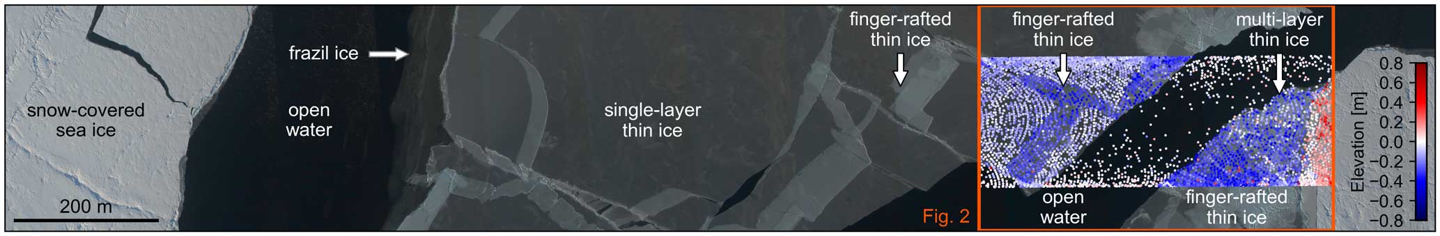
Figure 1Natural-color Digital Mapping System (DMS) image mosaic of sea ice in the Arctic Ocean north of the Beaufort Sea from 4 May 2016 (image center location N, W). Image spans 2020 m × 320 m. The location of Fig. 2 is indicated by the red outline. Coincident color-coded lidar point measurements are shown inside the Fig. 2 frame. Elevations are with respect to (w.r.t.) the mean elevation of the open-water surface. Lidar elevations over finger-rafted thin ice appear to be several tens of centimeters below the water surface. The mosaic shows different surface types discussed in this paper, including open water, newly formed thin ice, and snow-covered sea ice.
The primary observables of our study are apparent surface elevations and relative changes in pulse shape. We track biases in surface elevation by identifying measurements where the apparent ice surface elevation is lower than the elevation of open water in nearby measurements (Fig. 1). To complement our analysis of observed pulse shapes, we use a model of scattering of light in snow and ice (Smith et al., 2018) that predicts the shape of lidar waveforms reflecting from different snow and ice surfaces based on the shape of the transmitted pulse, the surface roughness, and the optical scattering properties of the medium. Any modeling of differential penetration over sea ice is challenging because both the physical properties of newly formed sea ice and its optical properties at 532 nm remain poorly known (e.g., Naumann et al., 2012; Zatko and Warren, 2015, and references herein). In general, grain size and absorbing impurities such as dust and black carbon are considered the two main factors contributing to variations in subsurface volume scattering over snow and ice (e.g., Gardner and Sharp, 2010; Flanner et al., 2012; Smith et al., 2018, and references therein). To address the unknowns related to the parameter space, our scattering model uses the mean distance Lscat a photon travels between effective isotropic scattering events as parameter, and together with varying surface roughness it determines the model waveform shape that best matches the shape of each observed waveform. To our knowledge no other study of differential penetration has been attempted over sea ice.
The analysis presented in this paper starts with a description of the airborne instruments and data sets we use (Sect. 2), followed by a description of the methods (Sect. 3). The observation part of our analysis presented in Sect. 4 depends on surface classifications for individual laser footprints and waveforms based on interpretation of visual appearance in coincident natural-color imagery. It also includes a discussion of potential other reasons for pulse broadening and elevation biases. Section 5 describes the model results, and Sect. 6 discusses the prevalence of differential penetration in lidar data over sea ice. Section 7 discusses the results in a broader context, and Sect. 8 concludes the paper.
This study utilizes data products from NASA's Operation IceBridge mission that have been well described in previous publications (e.g., Studinger et al., 2020, 2022b; Macgregor et al., 2021). We therefore only provide a brief summary of the main characteristics of the instruments and data products relevant to this investigation. More details can be found in the relevant user guides that, together with the data products, are freely available from the National Snow and Ice Data Center (NSIDC). Tables 1 and 2 summarize the airborne lidar and optical imagery instrument configurations used in this paper.
Table 1ATM laser altimeter configurations used in this paper.
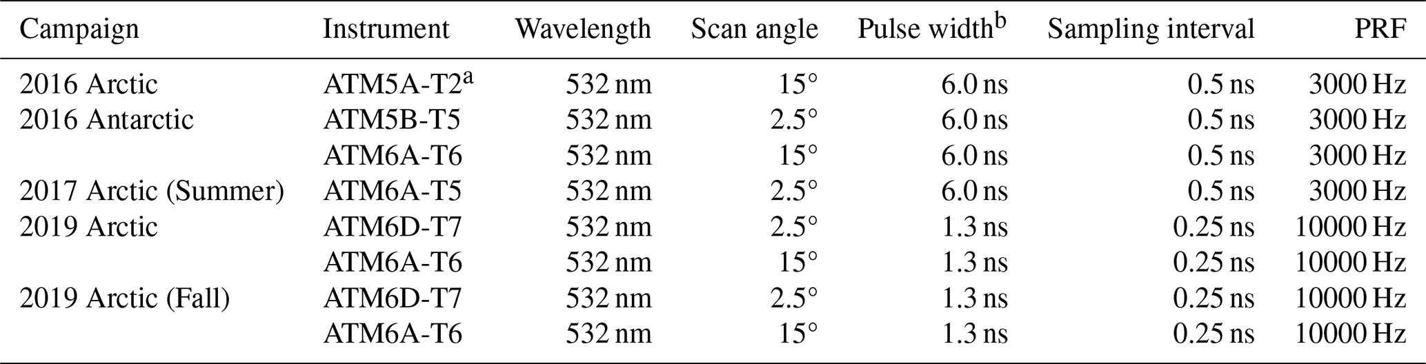
a For the 2016 Arctic campaign, the transceiver was mounted with the short axis across the swath for a single scanner deployment to increase data return over open water. b The nominal pulse width is measured as the full width at half maximum (FWHM) according to the factory specifications. PRF is the pulse repetition frequency.
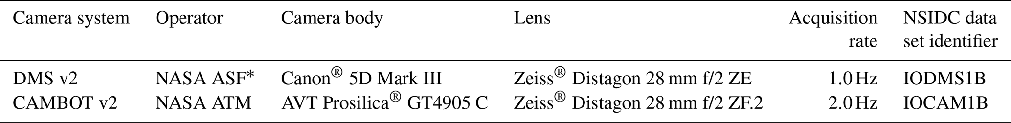
Table 2Camera systems used for natural-color optical imagery. ∗ ASF is the Airborne Sensor Facility at NASA's Ames Research Center.
In addition to the standard mission data products available from NSIDC, this study also uses ground calibration data and previously unpublished waveform data products from campaigns prior to standard waveform product delivery to NSIDC. These data sets, together with documentation and code to read the data, are made available through the Zenodo open data repository and are described below.
2.1 NASA's Airborne Topographic Mapper lidars
The Airborne Topographic Mapper (ATM) system consists of two independent laser altimeters (lidars) with different configurations to optimize data return over land and sea ice. Both systems are conically scanning lidars that measure the surface topography of a swath beneath the aircraft at a 15 or 2.5° off-nadir angle (Krabill et al., 2002). The ATM lidars used in this paper span four generations of ATM transceivers (T2, T5, T6, and T7), two generations of data systems (ATM5 and ATM6), and two generations of lasers (6 ns / 3 kHz and 1.3 ns / 10 kHz). Table 1 summarizes the lidar instrument configurations for the five campaigns used in this paper. We use the Level 1B geolocated point cloud data products (NSIDC data set identifier ILATM1B for the 15° scanners (Studinger, 2013) and ILNSA1B for the 2.5° narrow-swath scanners (Studinger, 2014). The Level 1B waveform products used for pulse shape analysis are available from NSIDC as ILATMW1B for the 15° wide scanner (Studinger, 2018a) and ILNSAW1B for the 2.5° narrow-swath scanners (Studinger, 2018b).
In addition to the airborne data, we use ground calibration (a.k.a. ground test) data for pulse shape analysis. These data are freely available from the Zenodo open data repository (Studinger et al., 2022a) for campaigns with corresponding waveform products at NSIDC. We also use ATM waveform data from the Arctic 2016 campaign before waveform data products were published through NSIDC. The waveform and ground calibration data for this campaign used here are freely available from the Zenodo open data repository (Studinger et al., 2023).
2.2 Natural-color optical imagery
For flights between 2009 and spring 2018 the Digital Mapping System (DMS), operated by NASA's Airborne Sensor Facility (ASF) at Ames Research Center (Dominguez, 2010), was the primary instrument for geolocated, orthorectified natural-color imagery (e.g., Macgregor et al., 2021). It was subsequently replaced by ATM's Continuous Airborne Mapping by Optical Translator (CAMBOT) system (Studinger and Harbeck, 2019) starting with the 2018 Antarctic campaign. Both systems are nadir-looking, three-channel (red, green, and blue, RGB) digital cameras with a 28 mm lens (Table 2). DMS and CAMBOT are both passive instruments that depend on natural sunlight for illuminating the area within the field of view (FOV) for imaging. Illumination depends on sun angle and cloud cover and often varies considerably during a flight. During sea ice missions the CAMBOT operator adjusts exposure parameters such as shutter speed, aperture, and sensor sensitivity (ISO number) to minimize motion blur and optimize exposure for the dynamic range of the camera sensor (Studinger et al., 2022b). Both systems have a cross-track FOV that exceeds the width of the ATM wide-swath scanner on the ground.
Data from both systems are used to produce geolocated, orthorectified images at 1 Hz, which, at the nominal ground speed of 140 ms−1, provides 60 % overlap between consecutive images for DMS and 80 % for CAMBOT, respectively (Macgregor et al., 2021). Both systems have similar ground resolutions of 10 cm (DMS) and 9 cm (CAMBOT) at a flight elevation of 460 m a.g.l. (Macgregor et al., 2021; Dominguez, 2010; Studinger and Harbeck, 2019). The geolocation accuracy is unspecified for both systems; however, visual comparisons between the orthorectified images and individual laser footprints presented in this paper shows that the geolocation accuracy over sea ice is sufficient for footprint-based lidar surface classification.
We use visual analysis of natural-color imagery to interpret the surface and ice type and combine it with the analysis and interpretation of co-located lidar-derived elevations and waveform characteristics.
3.1 Natural-color imagery ice type classification
We use the World Meteorological Organization (WMO) sea ice nomenclature that defines stages of formation and growth of sea ice based on visual appearance (World Meteorological Organization, 2014). Our analysis focuses on areas with new and young ice based on WMO's description and our interpretation of features visible in our natural-color imagery. This ice is less than 30 cm thick according to the WMO definition and has likely formed within a few days of freezing air temperatures over open-water leads. WMO's classification of new and young sea ice includes the following specific ice types. (1) The first type is made up of frazil ice and grease ice. Frazil ice consists of ice spicules or platelets that form in the top few centimeters of the ocean mixed layer and are considered the first stage of sea ice formation. In the absence of wind and waves, frazil ice crystals coalesce at the ocean surface into grease ice with a matte appearance (World Meteorological Organization, 2014). (2) The second type is made up of elastic layers of thin ice layers called nilas. The WMO classification of nilas distinguishes between dark nilas, which is typically less than 5 cm thick, and light nilas, which can be up to 10 cm thick. When pushed together under pressure, layers of nilas ice can form a distinct pattern of finger-rafted interlocking sheets. If further thickening occurs, nilas will turn into the third type, (3) gray ice, between 10 and 15 cm thick and gray-white ice that is 15 to 30 cm thick. We will discuss the differences in visual appearance and brightness related to ice thickness in our analysis. Because the interpretation of visual appearance of imagery is subjective and not always conclusive, we use the term thin ice or newly formed thin ice in this paper to discuss stages of ice formation that include the three different types of ice in the WMO definition of new and young ice. Our thin ice does not include WMO's thin first-year ice, which has a distinct visual appearance and is 30 to 70 cm thick. Figure 1 shows a natural-color, high-resolution (10 cm × 10 cm) mosaic of optical images. The mosaic shows several of the ice types discussed above and was coincidentally collected together with laser altimetry data along a flight line that will be discussed in Sect. 4.
3.2 Lidar data characteristics
The ATM instruments record digitized versions of both the transmit and return pulse that are provided in the mission data products ILNSA1B and ILATMW1B and are used for analysis here. Unlike the return pulse the recorded transmit pulse is routed through a multimode fiber-optic cable to separate the transmit pulse recording from the window reflection (Studinger et al., 2022b). The fiber-optic cable causes an instrument-related broadening of the pulse that we will address below. During survey flights, the transmit power of the lasers is kept constant, but variable neutral density filters in front of the detectors are adjusted during flight to optimize the dynamic range available from the 8-bit waveform digitizer (Studinger et al., 2022b).
3.2.1 Lidar elevations and return signal strength
To analyze and interpret ATM lidar elevations we utilize the elevation triplets provided with the mission data products ILNSA1B and ILATMW1B. These elevations are derived using the ATM tracking algorithm that determines the centroid of a laser pulse above an amplitude threshold for range determination (Studinger et al., 2022b). Data acquired with the 6.0 ns lasers uses 35 % of the maximum amplitude above the baseline as threshold, while data products from the newer 1.3 ns lasers use 15 % as amplitude threshold (Studinger et al., 2022b). The baseline is estimated from the median of the first 21 samples of the waveform. In addition to Studinger et al. (2022b), the MATLAB® functions used for ATM data handling and analyzing waveforms are available at https://doi.org/10.5281/zenodo.6341229 (Studinger, 2022). A Jupyter notebook demonstrating a Python™ implementation of the ATM centroid tracker is available at https://github.com/mstudinger/ATM-Centroid-Tracker (last access: 29 May 2024) (Studinger, 2024).
We also use the integrated signal strength of the lidar return pulse for analysis and interpretation. Because of the in-flight adjustment of the neutral density filters the signal strength is a relative measure. We estimate the relative return signal strength from trapezoidal numerical integration using the part of the waveform above a selected percentage of the maximum pulse amplitude above the signal baseline. For consistency with the ATM tracking algorithm, we use 15 % and 35 % as thresholds, respectively, and also 10 % to capture pulse broadening in the lower tail of the waveforms.
3.2.2 Pulse width and shape
The pulse width and shape of a return laser pulse, also known as the impulse response, is primarily a function of (1) the nominal transmit pulse, (2) instrument-related artifacts, and (3) geophysical interactions of the laser light with the surface and subsurface matter within the laser footprint on the ground. Because of the low flight elevations, we can neglect the effects of atmospheric scattering on pulse width and shape. The instrument-related alterations of the laser pulse are the combined result of characteristics of the photomultiplier detectors, various other system components such as optical delay fibers and instrument electronics and are common in waveform data of airborne and spaceborne lidars (Studinger et al., 2022b). To distinguish the signature in pulse width and shape caused by geophysical interactions from instrument-related artifacts we first determine the impulse response of the system using a calibration target. We record return waveforms on the ground for each campaign using a flat calibration target painted with Spectralon® that has no green penetration. Furthermore, surface roughness and slope within a footprint on the calibration target do not impact the shape of the return pulse and can be neglected (Studinger et al., 2022b). The recorded return waveforms are free of pulse-broadening effects from interactions with snow and ice targets and serve as a reference for comparison of waveforms over sea ice. The waveforms are aligned for averaging using the maximum of the cross-correlation between pulses with the signal baseline (noise floor) removed. To characterize pulse width, we estimate the pulse width at 15 % and 35 % of the maximum amplitude above the baseline consistent with the ATM centroid tracker and return signal strength estimates. Pulse widths estimated at lower amplitude thresholds are more sensitive to capturing photons that have experienced multiple scattering events along the optical path and therefore contribute to pulse broadening in the tail of the waveform. We also include a visual comparison of the shape of the waveforms over snow and ice targets relative to the reference calibration target on the ground.
Differential penetration is expected to vary with surface and ice type (Smith et al., 2018). Therefore, coincident, high-resolution optical imagery, co-located with the lidar point data, is critical as a visual reference for the analysis and interpretation of lidar data. The consistency in both space and time between the imagery and lidar data allows surface and ice type classification of individual laser footprints and waveforms for our analysis.
4.1 Differences in elevation, pulse width, and shape over various surface types
Figure 1 shows an example of different surface types in the Arctic Ocean during an Operation IceBridge (OIB) survey flight on 4 May 2016. The image mosaic, consisting of 18 partially overlapping three-channel, natural-color (red, green, and blue; RGB) images, spans 2020 m × 320 m with a pixel resolution of 10 cm × 10 cm. The image shows open water in two leads that appear as near black regions. The two leads are bounded by snow-covered sea ice with a very bright surface including shadows from pressure ridges formed by collision of ice floes. The strong brightness contrast in the natural-color imagery between snow-covered sea ice and open water is a result of the extreme contrast in spectrally averaged reflectivity of solar radiation (albedo) in direct sunlight between water and snow. Similarly, for laser light with a wavelength of 532 nm, the surface reflectance ranges from 0.05 to 0.2 over open water to 0.8 to 0.9 over snow-covered sea ice (e.g., Kwok et al., 2019). Using the WMO sea ice nomenclature of visual appearance (World Meteorological Organization, 2014), in between the two leads is an area of newly formed thin ice that is visible as a dark, gray surface. Abrupt changes in brightness, visible in several elongated features of increased brightness, is caused by rafting under pressure that pushes one ice layer over another and forming interlocking floes referred to as finger-rafted thin ice. The translucent nature of the thin ice allows both layers to be visible and we assume that the thickness of these areas of finger-rafted thin ice is approximately twice that of the single-layer thin ice. The brightest areas in the thin ice appear to be related to rafting involving more than two layers, and we refer to this type of sea ice as multi-layer finger-rafted ice (Fig. 1). In general, we observe that with increased levels of rafting the ice is more likely to optically look like snow-covered ice in terms of translucence and brightness.
To highlight the differences in visual appearance and lidar data between the different surface types we select a smaller area, covering 500 m × 320 m (Fig. 2). The location of Fig. 2 is marked by the red box in Fig. 1. Figure 2a shows a triangular-shaped area of gray-white ice (marked D) in the center right above the finger-rafted thin-ice area (marked B). We interpret this area as multi-layered thin ice with generally more than two layers rafted on top of each other. The lighter gray-white color compared to the single layer and finger-rafted thin ice comes primarily from buckling and ridges that form under pressure or from collisions of floes (Fig. 2a and b). We classify laser footprints, the spatial distribution of laser energy on the surface, based on the visual appearance of the natural-color imagery within the laser footprint and selected coherent regions with the same surface and ice type for analysis (Fig. 2b). Laser footprints in cyan are not used because they are either located near the edge of a feature and are therefore subject to classification errors associated with the geolocation uncertainty of the optical imagery and lidar data or are not located in an area with a homogenous surface type. We use identical color and symbol schemes for Figs. 2 to 4 for the surface and ice types discussed.
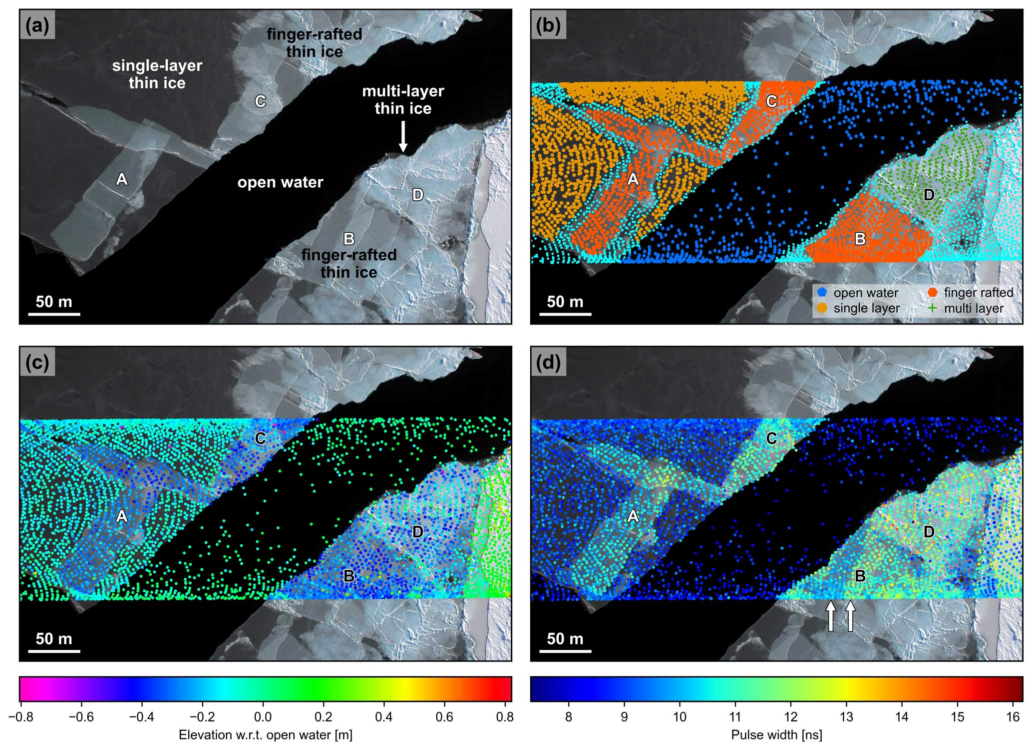
Figure 2(a) Natural-color DMS single frame of sea ice in the Arctic Ocean north of the Beaufort Sea from 4 May 2016 shown in Fig. 1 (location is indicated by the red outline in Fig. 1). Image spans 500 m × 320 m. (b) Surface classification of individual laser footprints. Laser footprints in cyan were not classified. (c) Elevation in meters w.r.t. open water calculated using data from the Level 1B airborne lidar product (ILATM1B). (d) Pulse width in nanoseconds estimated at 35 % of the maximum amplitude above the signal baseline. A pronounced change in pulse width related to the transition from single-layer to finger-rafted ice can be observed in area B (marked by two arrows in d). A version of Fig. 2 using color vision deficiency (CVD)-friendly color palettes for panels (c) and (d) is provided in Fig. A1.
Figure 2c shows that elevations with respect to (w.r.t.) water over thin-ice sections appear to be below the elevation of the open-water surface in leads. Elevation measurements shown in Figs. 2 and 3 are from the Level 1B airborne lidar product (ILATM1B) that assumes a propagation speed of laser light in air (Studinger, 2013). Within the thin-ice section on the left in the frame, there is a brighter T-shaped region (labeled A) where two to three layers of thin ice have been thrusted on top of each other. The brighter T-shaped area of finger-rafted thin ice shows elevations below the surrounding single-layer thin-ice area (Fig. 2c). The same effect can be seen in the area of finger-rafted thin ice right of the lead (labeled B). The natural-color image shows more complexity in the surface of the finger-rafted ice (labeled C) compared to features A and B. This area shows no distinct layers compared to A and B and appears to have characteristics from both finger-rafted and multi-layer thin ice. The brightness of this area is between that of the finger-rafted thin ice in A and B and the multi-layer thin ice in D. The multi-layer thin ice D is much brighter; appears to be less translucent than ice in areas A, B, and C; and shows elongated ridges along the edges of the ice floe. The small ridges cast shadows that are clearly visible in the imagery (Fig. 2a), indicating that this area is not submerged and is above the elevation of the adjacent open-water surface. The presence of ridges above the water surface and translucent areas corresponds to a mix of lidar elevations within this area that range from a few centimeters above that of the open water to ∼ 0.5 m below the water surface (Fig. 2c). To determine the pulse width of individual of individual return waveforms we first remove the baseline, calculated from the median of the first 21 samples of the waveform. Then, the time of the 35 % amplitude threshold is calculated using linear interpolation between the first sample below the amplitude threshold and the first sample above the amplitude threshold. This is done for both the leading edge and the tail of the waveform. The time difference between these two points is the pulse width at the desired threshold (Studinger et al., 2022b; Studinger, 2022, 2024). A map of pulse width (measured at 35 % of the maximum amplitude above the signal base line) shows a similar spatial pattern of differences between the different surface and ice types (Fig. 2d). Figure 2d shows that lower elevations generally coincide with broader pulse widths. The pulse broadening over finger-rafted ice relative to single-layer ice is visible in areas A, B, and C. A pronounced change in pulse width related to the transition from single-layer to finger-rafted ice can be observed in area B (marked by two arrows in Fig. 2d).
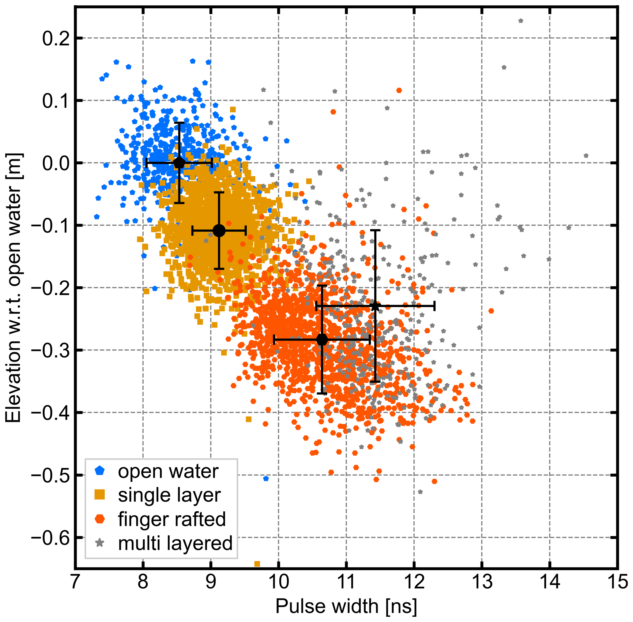
Figure 3Pulse width from Fig. 2d, estimated at 35 % of the maximum amplitude above the signal baseline, versus elevation w.r.t. open water for surface types shown in Fig. 2b. Elevation is from the Level 1B data product (ILATM1B), which assumes a propagation speed of laser light in air. The mean and standard deviation of the elevation and pulse width for each surface type are shown by black symbols and bars, respectively. The Pearson correlation coefficient of −0.7 for the entire point cloud indicates a strong negative correlation between pulse width and elevation w.r.t. open water.
The relationship between the pulse width from Fig. 2d, elevation, and surface and ice type is shown as a scatter plot in Fig. 3, where different surface types are represented by different symbol shapes and colors. We calculate the mean and standard deviation of the laser footprints for each surface and ice type shown in Fig. 2b. Relative to open water, the mean elevation of the single-layer ice is −0.11 ± 0.06 m, while the mean elevation of the finger-rafted ice is −0.28 ± 0.09 m. Elevations over single-layer thin ice are shifted below that of open water. The elevation shift is approximately twice as large over finger-rafted thin ice with two or more layers of thin ice and a total ice thickness presumably twice as that of the single-layer ice. The elevation shifts correspond to pulse broadening estimated at 35 % of the maximum amplitude above the signal baseline. The mean pulse broadening w.r.t. the mean pulse width over open water is 0.6 ns for the single-layer ice and 2.1 ns for the finger-rafted ice, respectively. Pulse broadening shifts the centroid of the reflected laser pulse to longer ranges and therefore lower elevations. The doubling of the elevation shift with the presumed doubling of the ice thickness suggests that pulse broadening happens along the optical path below the surface and within the thin ice layer(s).
The changes in pulse shape with surface and ice types relative to a penetration-free calibration target are shown in Fig. 4. The relative changes in pulse shape primarily result in the broadening of the pulse tail that is shown in Fig. 4. Figure 4a shows 548 474 stacked and normalized waveforms from the ground test range calibration for the campaign (Studinger et al., 2023). To average the waveforms the amplitudes of the individual waveforms are first normalized and then aligned using the delay estimated from the maximum of a cross-correlation between signals. Because the maximum of the cross-correlation does not always align with the maximum signal amplitude, the maximum of the stacked and averaged waveforms is slightly below 1.0. In order to enable a consistent comparison between the calibration target, ground test waveforms, and the airborne waveforms over ice and water, the averaged waveforms are normalized again. The pulse widths of the averaged waveforms at a desired threshold are then calculated as described in Figs. 2 and 3. The pulse shape of the instrument's impulse response from the range calibration target with no differential penetration shows deviations from a 6.0 ns (FWHM) Gaussian pulse because the transmitted laser pulse is not truly Gaussian and the combined instrument effects, such as detector characteristics, impact the recorded shape of the pulse, making it broader (Studinger et al., 2022b) (Fig. 4a). Instrument effects primarily change the shape of the pulse in the tail after the maximum signal amplitude, broadening the pulse in the tail section. Because of the pulse broadening, the centroid of the pulse, tc, occurs after the mean of the Gaussian at t=0 ns. Centroid times, estimated at amplitude thresholds of 15 % and 35 %, respectively, are marked in Fig. 4 for all panels. The range calibration waveforms are not affected by laser pulse interactions with natural targets and are therefore not impacted by differential penetration, surface roughness, or surface slope. Thus, we assess the changes in pulse shape over natural targets with respect to the shape of the range calibration waveforms. The shape and pulse width over open water from the lead in Figs. 2 and 3 is indistinguishable from the pulse width over the range calibration target 532 nm (Fig. 4a). The shift in centroid compared to the range calibration target is sensitive to the alignment of the waveforms. We use the maxima of the stacked and normalized waveforms as reference times. The shift in centroid compared to the range calibration target appears to be small. This suggests that the laser energy returned over open water comes primarily from the water surface. The return signal strength over open water is lower compared to the surrounding ice (Fig. A2). Depending on the angle of incidence, on a specular water surface some of the laser energy will be reflected away from the receiver and some will be refracted into the water, resulting in weak return signal strengths. Although 532 nm laser light penetrates water, the extreme low turbidity of the water results in low levels of laser energy returned from below the water surface that are not discernible in the recorded return laser pulses. Both the short pulse width and low return signal strength over open water support the interpretation that the elevation measurements over open-water areas observed in Figs. 2 and 3 represent the elevation of the water surface without a detectable bias from subsurface volume scattering.
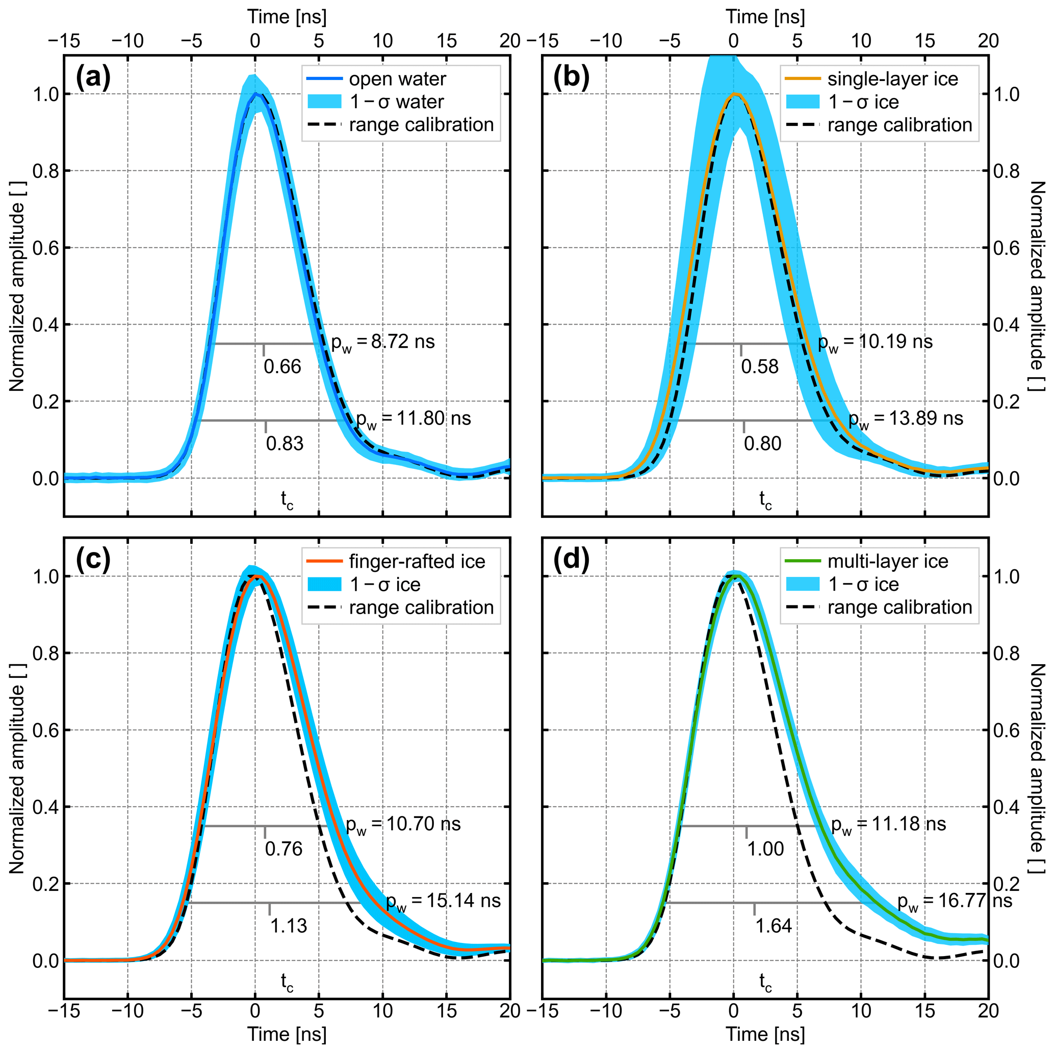
Figure 4Impulse response functions (IRFs) of the ATM5A-T2 transceiver determined from stacked, normalized return signal waveforms for different ice types and the ground test calibration. (a) Stacked and normalized return waveforms (blue line) over the open-water region shown in Fig. 2. The dashed black line in all panels shows stacked and normalized waveforms from the ground test range calibration over a flat, smooth target with no penetration shown for comparison. Ground test waveforms are within the same amplitude range as the respective airborne data used for comparison. The centroid of the pulse tc relative to the amplitude maximum and the pulse width pw are estimated at amplitude thresholds of 15 % and 35 %, respectively, and are marked by gray lines. The light blue shaded areas indicate the standard deviation (1-σ) of each sample of the stacked and normalized waveforms over ice and water. (b) Stacked waveforms over single-layer ice area. (c) The same information for finger-rafted ice. (d) The same information for multi-layered ice. The pulse shapes over thin ice in (c) and (d) show significant pulse broadening in the lower tail of the waveforms. The waveforms are aligned at the amplitude maximum.
The stacked waveforms in Fig. 4b show only a small shift in centroid location; however, the pulse appears to be broader than the pulse from the calibration target. The stacked waveforms in Fig. 4c and d, however, show significant pulse broadening and change in pulse shape over the finger-rafted and multi-layer thin ice sections. Most of the changes occur in the tail after the pulse maximum, but some changes in pulse shape are also visible in the leading edge before the maximum compared to the pulse shape from the calibration target with no penetration ( dashed black lines). The most significant changes occur in the lower part of the tail from photons that have traveled along a longer optical path. The associated shift in centroids results in longer slant ranges and therefore lower elevation measurements compared to open water.
4.2 Discussion of possible reasons for observed changes in elevation, pulse width, and pulse shape
We now consider possible reasons for the observed differences in elevation, pulse width, and pulse shape across different surface and ice types. The close spatial correlation between differences in observed elevations and pulse widths with surface and ice types in Fig. 2 suggests that geophysical interaction of green laser light with a given surface is the likely cause of observed elevation biases. However, we also consider the possibility of instrument and tracking algorithm artifacts and other geophysical phenomena such as melt ponds. To discuss possible reasons, we present additional examples of observed elevation biases involving several generations of the ATM instruments that also cover a broad spectrum of survey locations and conditions, such as time of year.
The first example shows sea ice 250 km north of the Svalbard archipelago in the Arctic Ocean from 20 April 2019 (Fig. 5). Unlike the data in Figs. 2–4, which used an earlier ATM system, this data set was acquired with two 1.3 ns short-pulse laser transceivers (ATM6A-T6 and ATM6D-T7). The point cloud of returns from the wide scanner (here ATM6A-T6) shows the typical absence of returns over open water because lidar energy reflected back from the water surface is a quasi-specular return due to the dielectric contrast between air and water (e.g., Wright et al., 2016). The 15° off-nadir scan angle results in most of the energy being reflected away from the transceiver. The remaining return energy that reaches the detector is typically below the trigger threshold of the digitizer. Here, the area of open water also includes barely visible frazil ice. To show the frazil ice, the image contrast in a 40 m × 40 m window was enhanced (Fig. 5a, white frame). The elevation bias is primarily visible on the narrow scanner (Fig. 5b, arrows), which is used as the primary altimeter over sea ice because the near-vertical angle of incidence of 2.5° results in returns from the water surface allowing freeboard estimates (Fig. 5b). Here, the elevations below the water surface occur over grease ice. The relationship between subsurface elevations and pulse widths (Fig. 6) for the narrow-scan data shows the shortest pulse widths over the water surface (15 to 90 m distance along profile because of the relatively smooth and leveled surface compared to the surrounding ice types). The subsurface elevations over grease ice between the distance of 75 to 90 m show significantly broader pulses than the water surface (Fig. 6). The short pulse width over open water also supports the argument that subsurface volume scattering of green laser light in open water within the ice pack can be neglected and does not seem to impact range and therefore elevation measurements. This is consistent with the observation in Fig. 4a that the pulse width over open water is nearly identical to the pulse width over a target without any known penetration. The fact that the open-water areas in this paper all appear as near black in natural-color imagery indicates a lack of submerged particles that could backscatter natural light or green laser light. A certain percentage of green laser light almost certainly penetrates into the water. However, the extreme low turbidity and lack of subsurface volume scattering support the interpretation that the lidar elevations over water surfaces in this paper are an unbiased reflection of the water surface elevation.
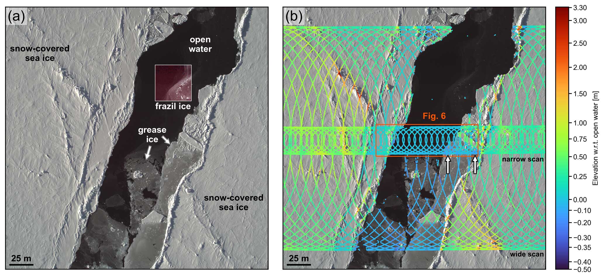
Figure 5(a) Natural-color CAMBOT image of sea ice 250 km north of the Svalbard archipelago in the Arctic Ocean from 20 April 2019 (image center location N, E). Image spans 290 m × 290 m. The image contrast in a 40 m × 40 m window (white frame) was enhanced to make the frazil ice in the upper few centimeters of the water visible. (b) ATM wide-scan (ATM6A-T6) and narrow-scan (ATM6D-T7) elevations w.r.t. open water. The location of the elevation profile shown in Fig. 6 is indicated by the red outline. The two arrows indicate locations of pulse broadening along the profile that is discussed in Fig. 6. An alternative version of Fig. 5 with a CVD-friendly color palette is provided in Fig. A3.
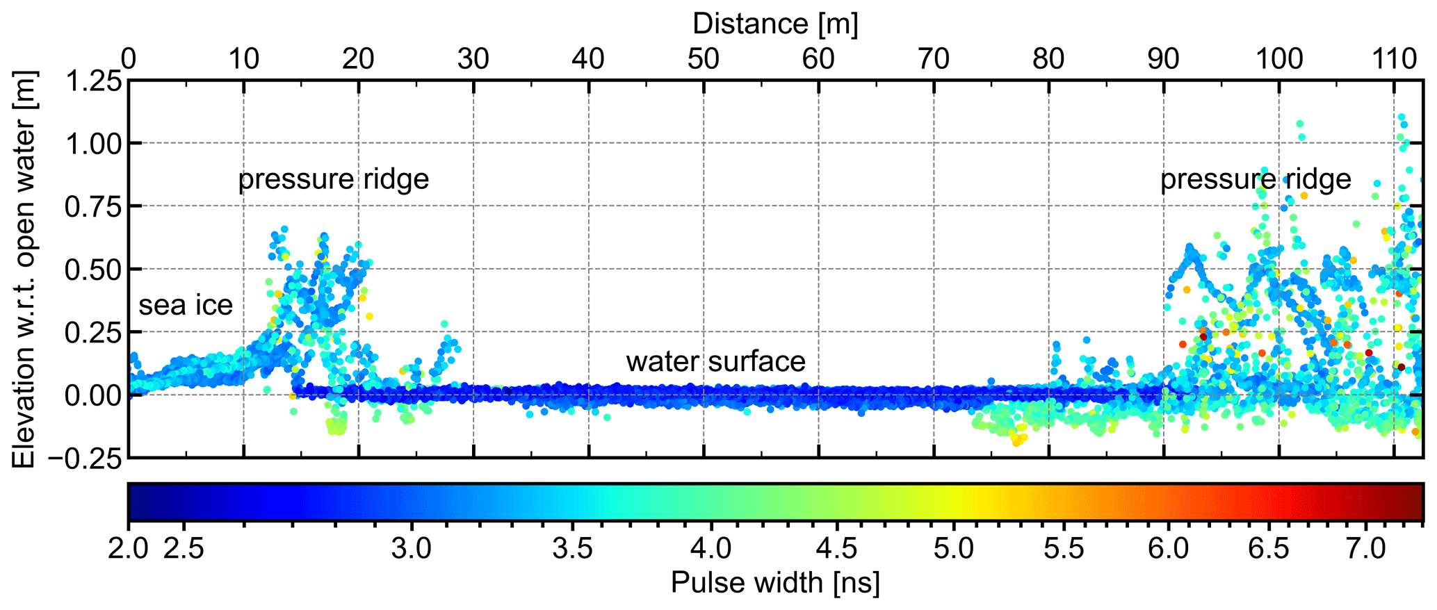
Figure 6Elevations w.r.t. open water of ATM narrow scan (ATM6D-T7). The location of the elevation profile is indicated in Fig. 5 by the red outline. Pulse width is estimated at an amplitude threshold of 35 % and shows pulse broadening of the elevations below the water surface, in particular the regions marked by arrows in Fig. 5 and at an along-profile distance of 75 m and more.
4.2.1 Instrument artifacts related to pulse shape
To rule out instrument artifacts as a possible cause, we now discuss instrument characteristics that alter the shape of the waveform. In general, instrument-related changes in pulse shape over the course of a campaign are the same for the return pulses recorded over the ground calibration target and over sea ice because the instrument does not change. Therefore, changes in return pulse shape over sea ice relative to the ground test waveforms are caused by geophysical interaction of the lidar pulse with the sea ice surface and subsurface. Both the qualitative comparison described in the previous section and the waveform modeling later described in Sect. 5 use the instrument impulse response determined over ground calibration targets for comparison with waveforms over sea ice. We can therefore rule out pulse broadening from instrument artifacts causing the observed changes in waveforms relative to the ground test waveforms (Fig. 4).
4.2.2 Tracking algorithm artifacts
ATM elevation data products use a centroid-based tracking algorithm to estimate the time of flight for range determination (Studinger et al., 2022b). For campaigns with waveform data products available from NSIDC (Studinger et al., 2022a), the centroid was estimated from the part of the pulse greater than 15 % of the maximum amplitude above the signal base level (Studinger et al., 2022b). For campaigns prior to that a 35 % threshold was used. As shown in Fig. 4, the laser ranges determined from the time of flight are sensitive to the threshold parameters used to estimate the time difference if pulse broadening occurs. In general, range estimates are sensitive to the particular method used, i.e., the tracking algorithm (e.g., Smith et al., 2018; Harding et al., 2011). The ATM calibration procedure for each campaign estimates and corrects the intensity-varying change in range known as range walk (Studinger et al., 2022b), and we can therefore rule out artifacts related to changes in return signal strength. Since we use relative changes in pulse shape and pulse width as primary observations to identify differential penetration, we can rule out the tracking algorithm artifact as an explanation for the observed elevation biases.
4.2.3 Surface slope and roughness
The slope and roughness of the illuminated surface area within the laser footprint on the ground can both cause broadening of the return pulse. Separating the effect of roughness and slope on the shape of a laser pulse is only possible when additional information such as the slope from a digital elevation model or overlapping lidar footprints is available (e.g., Brenner et al., 2012; Xie et al., 2022). Both surface roughness and slope are expected to broaden the laser pulse more or less symmetrically in the leading edge and the tail around the maximum of the pulse. This assumes that the height distribution within the area illuminated by the laser footprint has a normal distribution around a mean elevation. At the nominal flight elevation of ∼ 460 m a.g.l. the diameter of the ATM lidar footprints is 0.64 m for the data sets used in this paper (Studinger et al., 2022b). Our observations of anomalous elevations appear to occur primarily over newly formed thin ice and finger-rafted thin ice which are considered smooth and flat over length scales within the ATM footprint diameter. Furthermore, the conical scan geometry of the ATM laser altimeters creates a near-constant angle of incidence (Studinger et al., 2022b) over the flat, horizontal sea ice. Given the short flight times involved in covering the small data windows shown in this paper, aircraft attitude can be considered stable over the data windows and therefore not causing changes in the angle of incidence, which would impact the relative slope between the surface and the laser beam and therefore pulse width. We therefore rule out surface roughness and slope as having a significant effect on the observed spreading of the return pulse energy for the examples discussed in this paper. Since the pulse broadening here is only observed in the tail of the waveforms, the observed pulse spreading is inconsistent with pulse spreading expected from surface slope or roughness.
4.2.4 Flooding and submerged ice
We now consider the possibility that observed elevations below the water surface could be caused by laser energy reflected from flooded or submerged ice floes. The main purpose of altimetry measurements over sea ice is to derive ice thickness from freeboard measurements. This assumes that the sea ice is in hydrostatic equilibrium and has a lower density than the water. Therefore, the surface elevation of sea ice should be above the water level. While this assumption is generally considered to be valid for Arctic sea ice, sea ice in the Southern Hemisphere has long been considered more prone to flooding, with the sea ice having an elevation that is roughly the same as the water surface because of the combination of thinner ice, heavier loads from the overlying snow cover, and a larger fraction of marginal (lower concentration wave affected) ice (e.g., Kwok and Kacimi, 2018; Kurtz and Markus, 2012; Massom et al., 2001; Webster et al., 2018).
We analyze a sequence of loop-back repeat passes along CryoSat-2 orbit 34 602 in the southern Weddell Sea from 17 October 2016 that suggests that part of the sea ice is flooded and possibly submerged below the water surface although no snow cover is visible in the imagery. Figure 7 shows the elevation above the WGS 84 reference ellipsoid over a lead and sea ice that has been drifting over the course of the three passes at 19:28:53, 19:38:25, and 20:14:35 UTC. The optical imagery shows a difference in surface brightness of the ice north of the lead indicating that either the ice thickness or surface characteristic change. The well-defined shadows of small pieces of ice embedded in the ice in the bright areas in Fig. 7b and c (marked with arrows) indicate that the surface of the ice is not submerged and above water level (Fig. 7b). The gray ice in between the bright ice and the open water appears to be flooded. The smooth surface of this ice suggests it is very young and thin and elastic. The strongest evidence for flooding comes from a small, rafted piece of ice in Fig. 7c (marked with an arrow) that appears to bend the underlying ice with its load. The margin around this ice floe is darker, indicating increased water depth from the thin ice layer below that is deformed and pushed down by the weight of the rafted ice above (Fig. 7c). The change in surface elevation hw of the open water between passes indicates gentle wave action that could result in flooding of the marginal ice areas. There are no wind-induced capillary waves visible in the water in either optical imagery or lidar elevations (Fig. 7). The mean elevations hf of the lidar footprints over the flooded-ice area are 3.1, 2.8, and 2.6 cm below the mean elevations hw of the open water, respectively. The elevation change between the open-water and flooded-ice areas is small but consistent between the three passes flown in two different directions and at different times. While the ice appears to be very thin based on interpretation of its dark visual appearance, flooding of the pore space of the ice will likely increase the distance that the light penetrates below the surface, producing longer scattering delays and therefore lower apparent elevations. It remains unclear if the surface of the flooded ice is below the water surface or the apparent elevations below the water surface are caused by differential penetration or both. While it is possible to observe elevation biases over flooded ice, the small bias in elevation compared to the other examples in the paper and the presumably rare occurrence of flooded ice make it unlikely that flooding has a significant impact on freeboard and therefore ice thickness estimates, especially within the more consolidated Arctic ice pack. We cannot entirely rule out elevation biases caused by a flooded or submerged ice surface; however, the elevation biases are likely to be small and within the uncertainty of the lidar measurements.
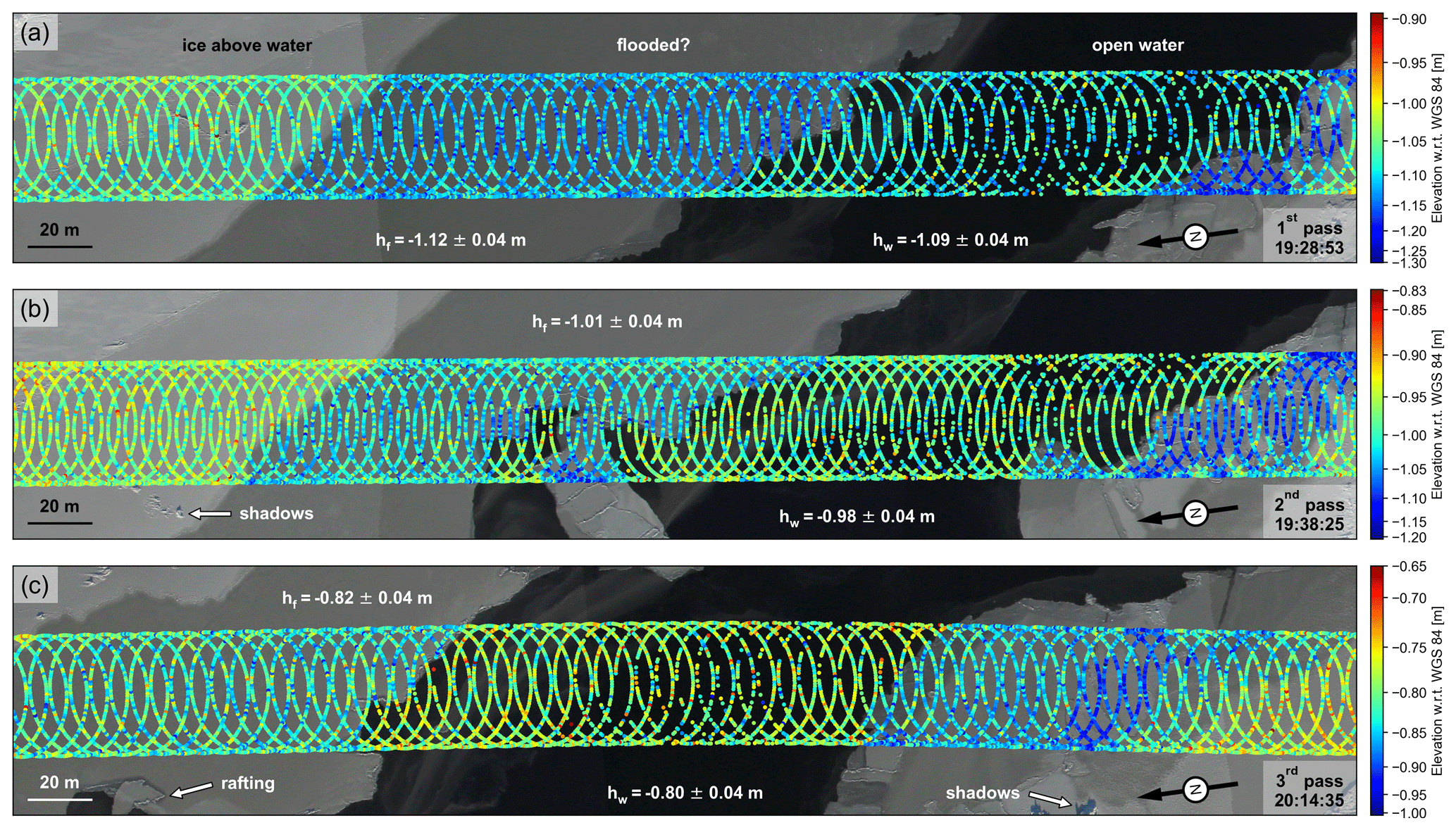
Figure 7Repeat passes over a segment in the southern Weddell Sea from 17 October 2016 (approximate location S, W). Each panel spans 430 m × 80 m with a pixel resolution of 10 cm × 10 cm. The UTC time of each pass is indicated in the lower right of each panel. Each panel shows natural-color DMS image mosaics and ATM narrow-scan (ATM5B-T5) lidar elevations above the WGS 84 (ITRF08) reference ellipsoid. Elevations are referenced to the WGS 84 ellipsoid to enable assessment of the changing open water elevation between passes. The survey aircraft is centered on the same ground reference track for each pass. Between the passes the sea ice drifted roughly subparallel along the orientation of the flight line, as can be seen in the image mosaics. The drift rates between passes were estimated from tracking the same sea ice feature in consecutive passes. The drift rate between the first and second pass is 480 m h−1 at 32° east–northeast (ENE, measured clockwise from true north) and 1780 m h−1 at 35° ENE between the second and third pass, respectively. The mean elevations above the WGS 84 reference ellipsoid and its 1-σ standard deviation are shown for the open-water (hw) and flooded-ice (hf) areas for each pass.
4.2.5 Melt ponds
During spring and summer melt ponds form over Arctic sea ice, further complicating the ice surface conditions. Over shallow melt ponds, 532 nm lidar returns can either be from the water surface, the water–ice interface at the bottom of the pond, or both when the water depth is shallow enough that the surface and bottom returns overlap (Studinger et al., 2022b). Lidar returns from the water–ice interface at the bottom of the ponds, so below the water surface, could be misinterpreted as being caused by differential penetration. A common approach to identify surface water on ice sheets and sea ice from natural-color RGB imagery is using the normalized difference water index modified for ice (NDWIice), which is defined as of the channels in an RGB image (Yang and Smith, 2013). NDWIice increases the spectral contrast between water and snow and ice surfaces for classification of water surfaces (e.g., Yang and Smith, 2013; Studinger et al., 2022b). Figure 8 shows a natural-color image of melt ponds over sea ice in the Lincoln Sea, the lidar elevation measurements, and the NDWIice surface classification using an NDWIice threshold of 0.2. The overlapping return pulses from the surface (S) and bottom (B) in the shallow part of the melt pond result in an apparent elevation bias from ATM's centroid tracker, which is designed for ice surface elevations and does not separate the surface and bottom pulses (Fig. 9a) like a dual-peak Gaussian tracker (blue dashed line in Fig. 9a) designed for bathymetry estimates (Studinger et al., 2022b). The slant range in water estimated from a Gaussian waveform fit of the two distinct peaks is 0.28 m and is close to the minimum detection threshold of 0.30 m for this approach estimated by Studinger et al. (2022b). For deeper parts of the melt pond with a slant range in water of 1.52 m, the surface and return pulse are separate (Fig. 9b).
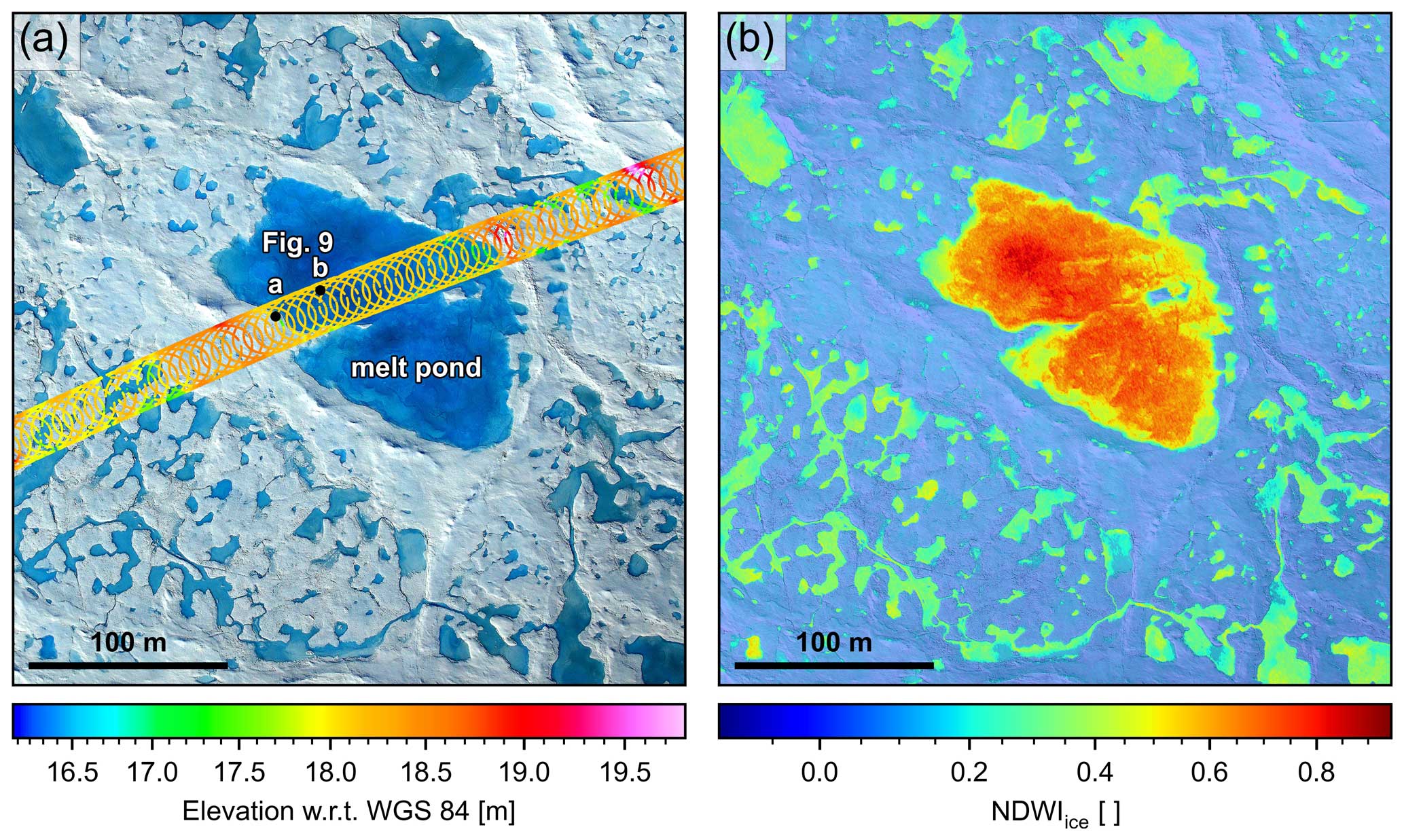
Figure 8(a) Natural-color (RGB) imagery with ATM6AT5 lidar elevation measurements from 25 July 2017 in the Lincoln Sea north of Ellesmere Island showing melt ponds, meltwater channels, and snow-covered sea ice. Locations of example waveforms shown in Fig. 9 are marked by black dots. (b) NDWIice highlighting melt ponds and liquid water on the surface. An alternative version of Fig. 8 with CVD-friendly color palettes is provided in Fig. A4.
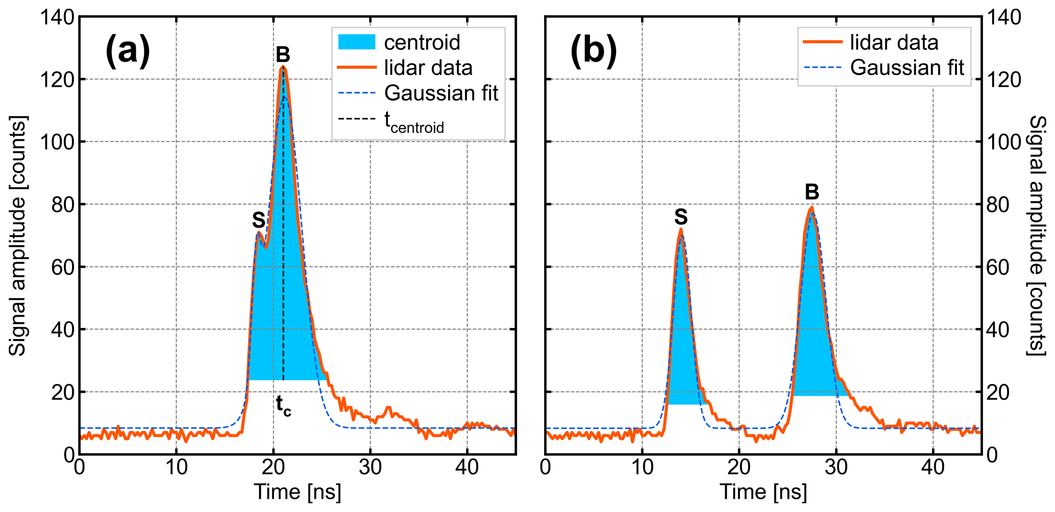
Figure 9Lidar waveforms over the melt pond shown in Fig. 8. (a) Gaussian fit of two peaks of overlapping surface (S) and bottom (B) return pulses. The slant range in water between the surface and bottom return pulses is 0.28 m. (b) Laser energy reflected from the surface and bottom appears in two separate pulses for the deeper part of the melt pond. The slant range in water is 1.52 m.
The lower elevations from overlapping pulses and bottom returns could be misinterpreted as pulse broadening. However, the pulse broadening of overlapping pulse is significantly larger than previously described and the two distinct pulses for deeper melt ponds allow a clear separation from the previously described effect together with the visual appearance of the melt ponds in natural-color imagery. We therefore rule out melt ponds as being mistaken for differential penetration over sea ice.
4.2.6 Subsurface volume scattering
In conclusion, we consider subsurface volume scattering as the most likely reason for the observed relative changes in pulse width and shape causing the observed elevation biases discussed in this paper. Over snow and ice, green laser light can penetrate below the surface where photons then experience multiple scattering events within the medium before returning to the surface. The lengthening of the optical path from multiple scattering results in a time delay that translates into a range delay. The actual bias in elevations derived from waveform data not only depends on the volume scattering but also on the tracking algorithm and the threshold used to select the part of the pulse used for range determination (e.g., Smith et al., 2018; Harding et al., 2011; Ricker et al., 2014). In addition to that the amount of back-scattered energy that contributes to the signal strength and therefore pulse broadening in the lower tail also depends on the FOV of the telescope and the alignment of the laser footprint with the telescope's FOV during data acquisition, in part because photons that have experienced multiple scattering events are more likely to experience lateral spreading away from the center of the laser footprint. A larger field of view will capture more of these photons, thus impacting the observed elevation. Because of the harsh environmental conditions inside an aircraft during survey flights in polar regions the alignment between the FOV of the telescope and the laser needs to be adjusted during flight. A consequence of the changing alignment is that it will be difficult to determine an elevation bias correction to the laser measurements that properly accounts for differential penetration. In the next section we attempt to model the effect of subsurface volume scattering on the shape of the lidar waveforms and estimate the elevation bias resulting from subsurface scattering based on a range of physical and optical parameters.
To help interpret the physical mechanism behind the apparent volume scattering, we match the waveform shapes with a model of scattering of light in snow and ice (Smith et al., 2018) that predicts the shape of lidar waveforms reflecting from snow and ice surfaces based on an estimate of the ATM impulse response function (IRF), the surface roughness, and the optical scattering properties of the medium. Because we do not know the density or grain size of the ice and snow measured by ATM, we parameterize the scattering in our model based on Lscat, the mean distance a photon travels between effective isotropic scattering events, assuming that the velocity in the medium is equal to that in air. In snow, a longer scattering length corresponds to lower density, larger grain size, or the presence of liquid water (which tends to suppress scattering). In ice, a longer scattering length corresponds to higher density or smaller bubbles, and we expect to see small or zero recovered scattering length for returns from impenetrable surfaces or from open water. To interpret the returns, we generate model waveform shape estimates for a range of surface roughness and Lscat values and select the model waveform shape for each measured waveform with the smallest least-squares misfit. The fitting process is described in detail in the companion paper (Smith et al., 2023). The companion paper includes an approach to correct elevation measurements for land ice altimetry data, which is not adequate for correcting sea ice elevations. Developing such a correction is challenging, as described in Smith et al. (2023), and beyond the scope of this paper.
For the first example we use lidar data from an attempted underflight of ICESat-2 on 9 September 2019 in the Wandel Sea north of Kalaallit Nunaat (Greenland) with various surface types in the optical image including open water, thin ice, and snow-covered sea ice (Fig. 10). The lidar data from the ATM narrow scan (ATM6D-T7) shows elevations below the water surface in a narrow band over thin ice marked by arrows (Fig. 10b). Figure 10c shows a map of the recovered scattering lengths Lscat.
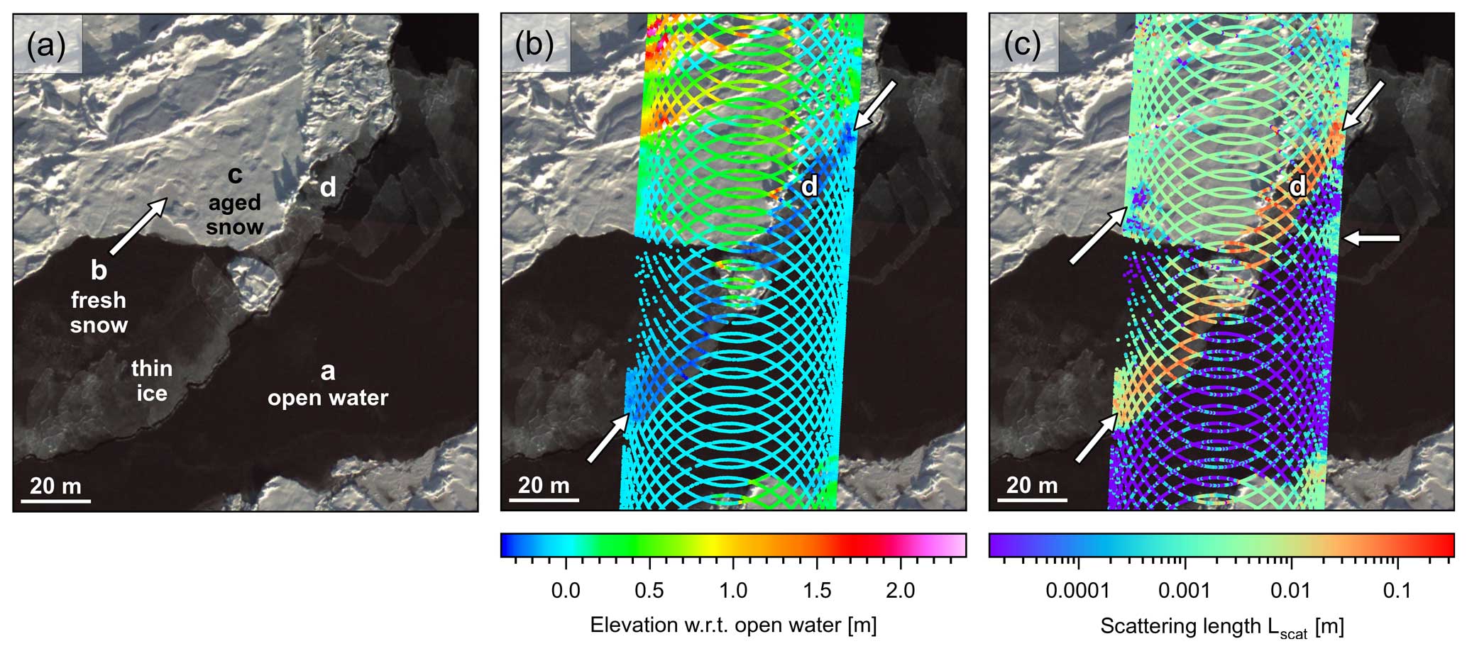
Figure 10(a) Natural-color CAMBOT image of sea ice in the Wandel Sea from 9 September 2019 (image center location is N, W). Image spans 140 m × 150 m with a pixel resolution of 20 cm × 20 cm due to higher-than-normal flight elevation. Labels in lower case letters in panels (a) to (c) are as follows: a is open water, b is fresh snow, c is aged snow, d is thin ice. These indicate locations of lidar and model waveforms shown in Fig. 11. (b) ATM narrow-scan (ATM6D-T7) elevations w.r.t. open water. (c) Modeled scattering length (Lscat) showing longer scattering lengths over thin ice. A band of thin ice elevations below the water surface is marked by arrows in panel (b) and shows longer scattering lengths (marked by arrows). The location of the image frame is shown in Fig. 13. An alternative version of Fig. 10 with a CVD-friendly color palette is provided in Fig. A5.
Figure 11 shows model waveforms and ATM lidar waveforms for select locations marked a–d in Fig. 10. The modeled waveforms are generated by convolving an estimate of the IRF from calibration measurements with the distribution of returned photons predicted by the model for each grain size. The dashed red lines mark the location of the centroid of the observed waveform relative to the model surface elevation and therefore reflect the range biases. The hbias values are the centroid-based range biases from the observed waveforms (dashed red lines) corrected for the angle of incidence and therefore reflect the estimated elevation bias relative to the model surface. Misfits between observed waveforms and model waveforms are consistently small, implying that our model adequately simulates the most important features of the scattering processes (Fig. 11).
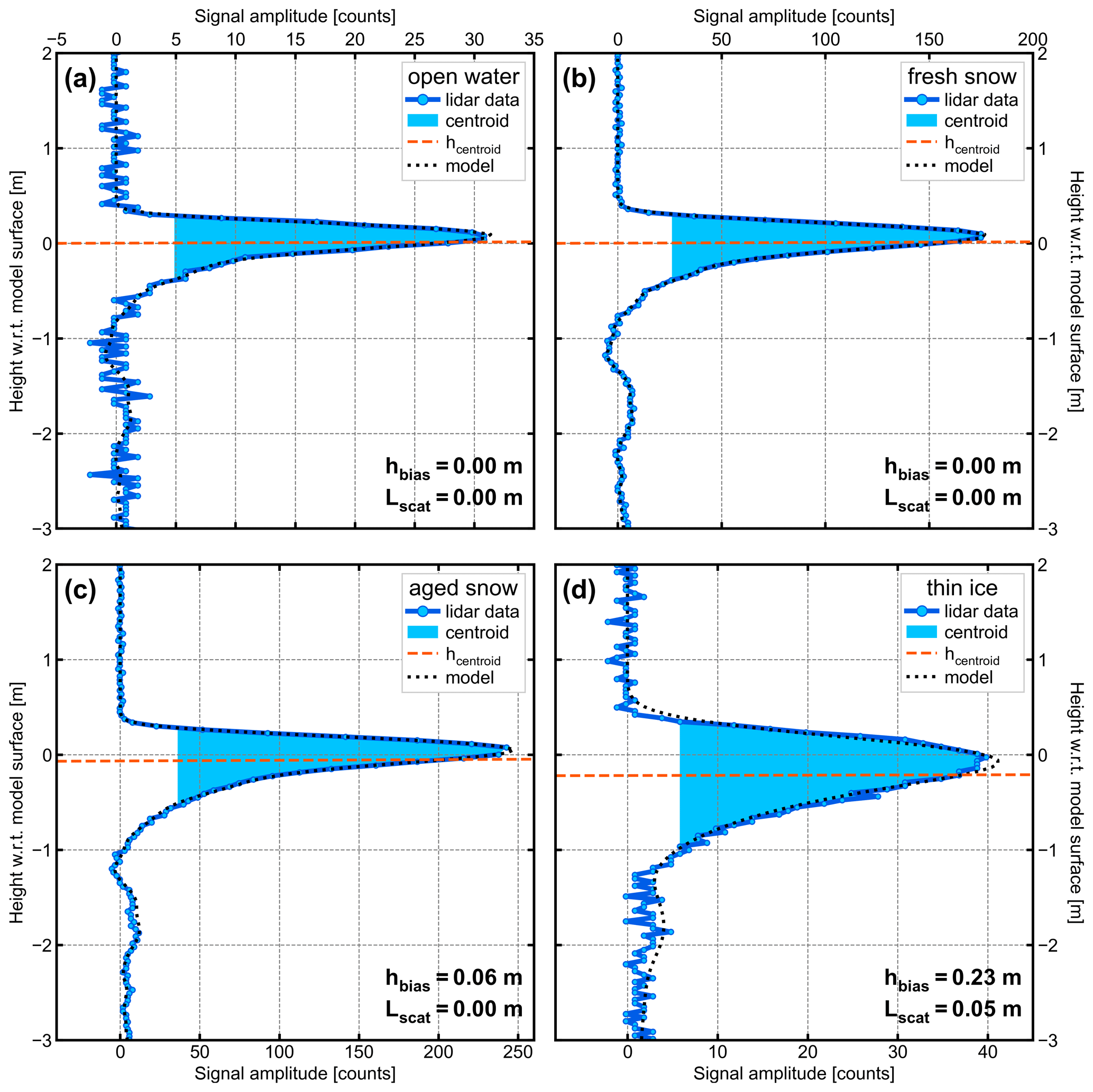
Figure 11Modeled waveforms (dotted black lines) with observed ATM lidar waveforms (blue lines, dots indicate location of data samples). For locations see Fig. 10a. Figure 10c shows a map of the recovered scattering lengths for the area shown in Fig. 10a. The dashed red lines mark the location of the centroid of the observed waveform relative to the model surface elevation. The hbias values are the centroid-based range biases from the observed waveforms (dashed red lines) corrected for the angle of incidence and therefore reflect the estimated elevation bias relative to the model surface. Over open water (a) our fitting procedure recovers a scattering length Lscat=0 m, as expected for Fresnel reflections with little subsurface scattering. Likewise, for fresh snow that has accumulated in hollows in the sea ice (b), the scattering length is near 0 m. For aged snow on the sea ice (c), Lscat values are around a few millimeters, which is a reasonable value for snow with a density of 300–400 kg m−3 and grain sizes on the order of 100–500 µm. The largest scattering lengths were found for the thin ice that exhibited the largest negative altimetry biases (d), where scattering lengths of 3–5 cm allow photons to build up considerable range biases (hbias) over multiple scattering events. Misfits between recovered waveforms and model waveforms were consistently small, implying that our model adequately simulates the most important features of the scattering processes.
Over open water (labeled a) our fitting procedure recovers Lscat=0 m, as expected for Fresnel reflections with little subsurface scattering. Likewise, for fresh snow that had accumulated in hollows in the sea ice (labeled b), the scattering length is 0 or near 0 m (and marked by the arrow in panel c). For aged snow on the sea ice (labeled c), we find Lscat values are around a few millimeters, which is a reasonable value for snow with a density of 300–400 kg m−2 and grain sizes on the order of 100–500 µm. The largest scattering lengths are found for the thin ice that exhibited the largest negative altimetry biases (labeled d), where scattering lengths of 3–5 cm allow photons to build up considerable range biases over multiple scattering events.
The elevation bias hbias estimated from the model range bias for the thin ice in Fig. 11d is 22 cm and similar in magnitude to the elevation bias over thin ice in ATM data shown in Fig. 10b and provides confidence for our interpretation of both the modeling results and observations.
The second example of our scattering model is applied over slightly different ice types and uses the data north of the Svalbard archipelago shown in Fig. 5. Here we model waveforms from both the wide- and narrow-scan lidars (Fig. 12). We use this example to highlight subtleties the model is capable of resolving but also show situations when the scattering model should not be used to model differential penetration. The modeled scattering lengths for narrow-scan waveforms over open water are close to zero as expected, indicating that there is very little laser energy coming back from below the water surface (Fig. 12). Over grease ice, scattering lengths are much higher, reaching several centimeters in both the wide-scan and narrow-scan data. The area between the arrows with below-surface elevations shown in Fig. 6 is consistent with longer scattering lengths (Fig. 12). The largest scattering lengths of several tens of centimeters are near the edge of the wide-scan swath (left and below the location of the inset map), but here the observed pulse broadening may be a result of surface roughness in addition to differential penetration.
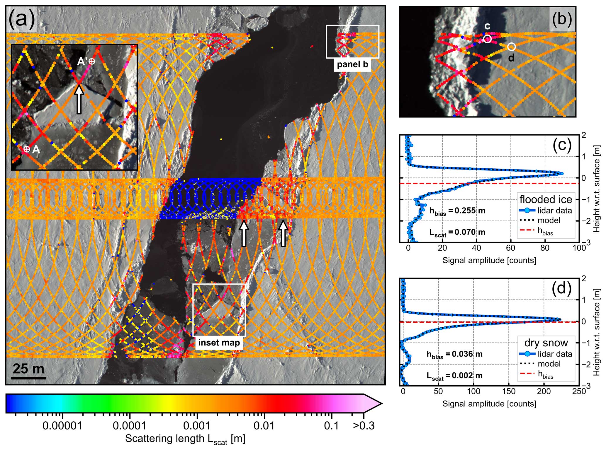
Figure 12(a) Modeled scattering length (Lscat) for the data north of the Svalbard archipelago shown in Fig. 5. See the text for a discussion of the inset map marked by the white square. An elevation profile across a small ice floe along the lidar scan line from A to A′ is shown in Fig. A2 and discussed in the text. (b) Detail of modeled scattering length next to a pressure ridge. Color scale is the same as in (a). The locations of waveforms shown in panels (c) and (d) is indicated by small white circles. (c and d) Modeled waveforms (dotted black lines) with observed ATM lidar waveforms (blue lines, dots indicate location of data samples) for the two locations marked in (b).
Another example from this location shows how interpretation of visual imagery can be enhanced using scattering length information. Waveforms next to a pressure ridge inside an area outlined by a white box are shown in Fig. 12b. There is a pronounced increase in apparent scattering length closer to the pressure ridge (note that this change does not appear to coincide with the light–shadow transition). The change in scattering lengths reflects differences in waveforms shown in Fig. 12c and d. The waveform Fig. 12d is over what appears to be dry snow in the optical image (Fig. 12b) and is typical for dry snow. The example waveform and scattering model closer to the pressure ridge (Fig. 12c) is much broader with longer scattering lengths resulting in a significant modeled elevation bias of 25 cm. The region within the shadow with longer scattering lengths is a slightly darker area. We interpret this area as potentially having been flooded, which would result in longer scattering lengths as observed. The flooding could have been caused by the load of the pressure ridge depressing the surrounding ice below the water surface.
A small ice flow inside the wide-scan swath shows the model performance across different ice types and surface conditions (Fig. 12a inset map). The scattering lengths along a scan line over the ice floe from A to A' shown in Fig. A6 shows higher scattering lengths and negative elevations (w.r.t. open water) over the grease ice surrounding the small ice floe. The isolated large Lscat values near the edge of the floe are an artifact of complex surface topography within the lidar footprint and not related to differential penetration. An example of this effect is shown in the inset map in Fig. 12a (arrow) and Fig. A6. The waveform at the edge of the ice floe along the scan line from A to A' (Fig. A6) has two distinct peaks indicating that this lidar footprint is over complex surface topography with high surface roughness and the observed pulse broadening is not caused by differential penetration. Like the waveform over the melt pond in Fig. 9a, the presence of two peaks in the lidar waveform near the edge of the ice floe can be used to distinguish such waveforms from the effect of differential penetration. The visual appearance of the ice floe in the imagery (Fig. 12a) and the elevation profile (Fig. A6) show that the surface of ice floe appears to be tilted with a slope. The expected low Lscat values over the ice floe suggest that the slope has no significant impact on the modeled scattering lengths over the floe.
Discussion of modeling results
The close correspondence between long scattering lengths and negative elevation values (w.r.t. open water) suggests that subsurface scattering is the likely reason for these negative values. It is likely that there is also some penetration bias on the snow-covered floes, but because the grain sizes are smaller (leading to smaller biases) and the snow surface is higher, these are not as obvious as the biases on the thin ice.
Our model performs best for the most recent subset of the ATM data. The 6.0 ns pulse widths used by the system before the Arctic summer 2017 field season limit the range of grain sizes for that produce noticeable changes in the return shape. For the coarsest-grained ice, with the largest scattering lengths, the shape of the trailing edge of the pulse can change (e.g., Fig. 4c and d), but these changes may not always be clearly distinct from the effects of roughness. For the 1.3 ns pulse lasers the pulse shape is much more sensitive to surface conditions. The presence of large amounts of dust or algae in ice or snow would also tend to reduce the scattering length estimated from our model because it would reduce the intensity of the return in the later part of the return. The camera images suggest that the ice was fairly clean in the data presented in this study, and there was no obvious source of particulate matter or soot, so we do not believe that this played a large role in our results. A more serious limitation of the model is its assumption that the returned light scattered from a semi-infinite medium, when the actual ice may be thin or may include multiple layers. When the ice is optically thin, the model likely estimates scattering lengths that are smaller than the scattering length in the ice (because photons that travel long distances are lost from the bottom of the ice), while in layered ice, the estimated scattering lengths likely reflect an average for the near-surface region, with the averaging length depending on the grain size of the snow.
Several algorithms exist for detecting leads and melt ponds over sea using high-resolution, natural-color (RGB) imagery (e.g., Buckley et al., 2020; Onana et al., 2013; Wright and Polashenski, 2018). Existing surface classification algorithms are based on the analysis and interpretation of RGB or NDWIice (Yang and Smith, 2013) pixels and histograms (e.g., Buckley et al., 2020). Some use signal transformations (Onana et al., 2013) or training data sets and object-based classifications (Wright and Polashenski, 2018). The primary motivation for developing these algorithms was the detection of leads and melt ponds over Arctic sea ice. The existing algorithms developed for OIB imagery data products have all in common that they apply a set of decision criteria on a frame-by-frame basis (Onana et al., 2013; Wright and Polashenski, 2018; Buckley et al., 2020). Both the DMS and CAMBOT systems used for OIB use the camera's auto-exposure function that adjusts shutter speed, lens aperture, and the camera's sensitivity to light to optimize exposure over the dynamic range of the camera's sensor (Studinger et al., 2022b). As a result, changes in brightness within the camera's FOV results in different exposures for neighboring image frames, which can cause different surface classifications for the same thin ice type between two overlapping image frames. While lead and melt pond detection can work well (e.g., Fig. 8), classification of thin ice remains a challenge. The examples shown in this paper are all RGB color images, but with the exception of Fig. 8 have the appearance of grayscale images, which reflects the lack of spectral contrast between surface types that could be used for classification, excluding melt ponds that have a small water depth and a blueish color (Fig. 8). Furthermore, the very subtle differences in brightness and spectral appearance between thin ice and open water vary with changing sun illumination (high-angle and low-angle sun, direct and diffuse light, clouds), lens vignetting, and changes in instrument configurations over the course of the OIB mission (e.g., Macgregor et al., 2021; Studinger et al., 2022b). Developing a robust algorithm for the detection of various types of young ice described in this paper that would allow a comprehensive assessment how prevalent these ice types and associated elevation anomalies are is beyond the scope of this paper given the complexities involved.
To estimate how frequent thin ice sections with lidar elevations below the water surface occur we have manually analyzed an entire OIB flight. We chose the attempted ICESat-2 underflight during OIB from 9 September 2019 in the Wandel Sea north of Kalaallit Nunaat (Greenland; Fig. 10) because of the intended coincident spatial and temporal data collection between ICESat-2 and ATM. Data collection was organized in six parallel flight lines each 230 km long and centered on ICESat-2 ground reference tracks. The six lines were flown in two groups of three lines, with the center lines of the groups spaced 3.25 km apart and centered on an ICESat-2 strong beam (GT2R and GT3R for this date), resulting in overlapping natural-color imagery and near-complete lidar coverage between neighboring segments each separated by 0.42 km. We have analyzed 4965 geolocated CAMBOT L1B images along the six lines together with ATM lidar data and have marked frames with thin ice and lidar elevations below the water surface similar to Fig. 10. The locations are plotted in Fig. 13 (light blue circles). We have excluded neighboring frames in overlapping CAMBOT images that appear to cover the same feature. Several of the identified leads appear to have drifted to the neighboring survey line over the course of the flight and were surveyed twice. We have not excluded these occurrences since they seem to be rare. We have identified 180 occurrences of thin ice sections in the 9 September 2019 data (Fig. 13) where lidar elevations appear to be below the water surface based on visual interpretation of CAMBOT imagery and lidar data. The number of thin ice sections in this flight and the multitude of examples presented in this paper from different instrument generations, regions, and times of year suggests that subsurface volume scattering over sea ice resulting in elevation biases are not rare, isolated occurrences but are likely more prevalent in OIB data than previously assumed.
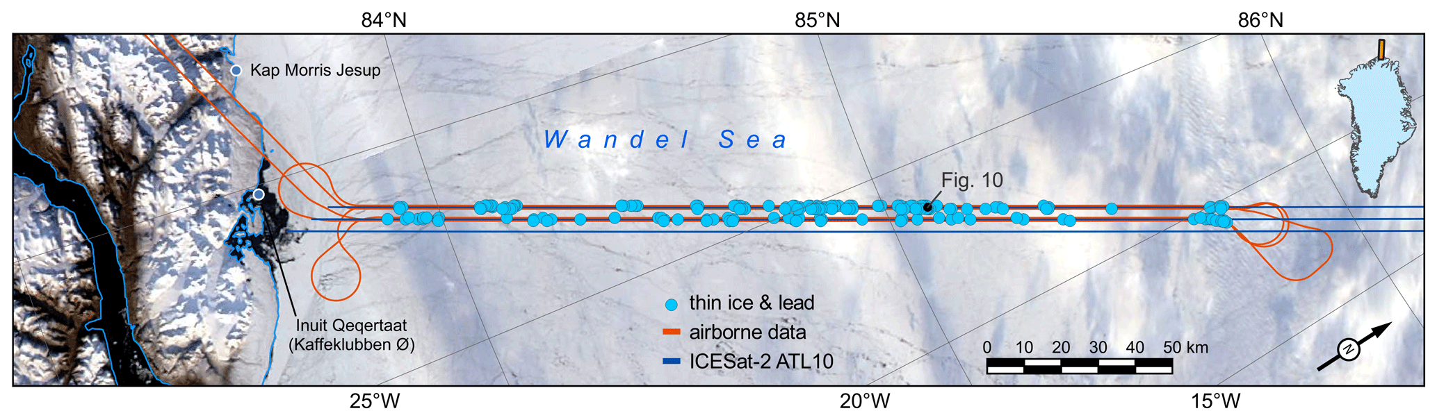
Figure 13NASA Operation IceBridge airborne data from 9 September 2019 (red lines) during an attempted underflight of ICESat-2 in the Wandel Sea north of Kalaallit Nunaat (Greenland). At the time of the overpass the survey aircraft was unfortunately not located over an ICESat-2 beam (dark blue lines) and no truly coincident data exist. Light blue circles indicate where subsurface elevations over thin ice adjacent to leads have been identified in airborne data. Background is an Aqua true-color image mosaic of corrected reflectance from 9 September 2019 (NASA Worldview Earthdata, 2019). Blue lines indicate locations of ICESat-2 ATL10 data (Kwok et al., 2023) along the six ICESat-2 ground reference tracks. Inset map shows location of main map area north of Kalaallit Nunaat (Greenland).
While the focus of this paper is on identifying differential penetration in ATM data over sea ice, the fundamental physics of how green laser light interacts with geophysical targets is independent from the science instrument and suggests that broader ramifications of this effect may exist across lidar missions. As previously discussed, instrument design and tracking algorithms will add instrument and algorithm specific effects, but they do not change the geophysical interactions between green photons and ice targets. Therefore, it is likely that differential penetration over ice exists in other 532 nm lidar data. For example, Smith et al. (2023) discusses elevation biases in ICESat-2 data over the Greenland Ice Sheet that are caused by subsurface scattering of green photons and its variation with grain size. In general, the scattering length Lscat we use in our model is roughly proportional to the grain size and inversely proportional to the density. The largest factor driving variability in the scattering length is grain size, since grain size varies over several orders of magnitude between snow and ice, while changes in density between different ice types are very small. While a comprehensive analysis is beyond the scope of this paper, we have undertaken an exploratory analysis of the ICESat-2 sea ice data (Kwok et al., 2023) that covers the near coincident data acquisition with ATM on 9 September 2019 (Fig. 13). When ICESat-2 freeboard calculations result in a negative freeboard these values (150 photon aggregated segments in the sea ice products) are being set to zero in the ICESat-2 ATL10 data product. However, it is possible to use the information in the ATL10 data to “restore” these negative freeboard values that were set to zero. This is done by subtracting the ATL10 surface height segment data also reported in ATL10 from the freeboard values for non-negative values of freeboard to determine the sea surface height at the given segment. A linear interpolation of this sea surface height is then done to points with a freeboard value equal to zero and then subtracted from the respective ATL10 surface height to “restore” the negative freeboard value. Using these data, we can then evaluate if a similar relationship between subsurface elevations (negative freeboard) and “pulse width” can be seen in ATL10 data. The “height_segment_w_gaussian” in ATL10 data, which is the width of the best fit Gaussian convolved with the ICESat-2 impulse response, is comparable to the scattering surface pulse width of a conventional lidar and potentially indicates subsurface volume scattering in a photon-counting lidar system. We limit our analysis to finite pulse widths > 0.05 m and freeboard < −0.04 m, which is outside the 2-σ noise of the ATL10 data.
We did not identify negative freeboard values near the locations identified in the ATM data (Fig. 13) but have found several occurrences in the same data tile along its northeastern extension outside the airborne survey area. Negative freeboard plotted versus the Gaussian fit width (Fig. 14) shows a similar relationship to that between the elevations w.r.t. water surface versus pulse width for the ATM data (Fig. 3): the pulse width determined from the Gaussian fit width appears to increase with decreasing elevations below the water surface (“negative freeboard”) suggesting that this relationship may reflect differential penetration of green photons into ice.
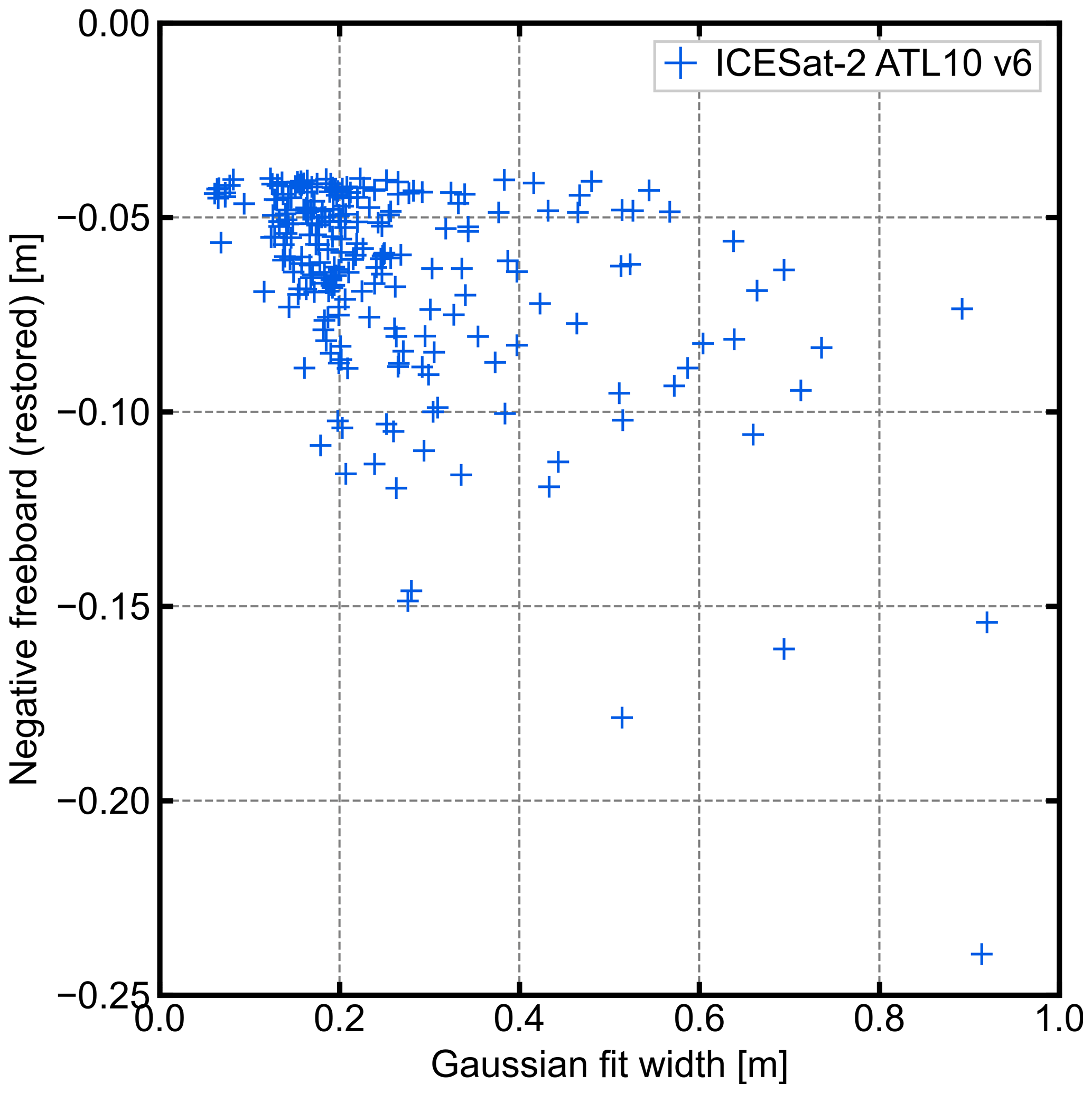
Figure 14Negative freeboard restored from ICESat-2 ATL10 data (Kwok et al., 2023) plotted versus the Gaussian fit width representing the scattering surface “pulse width” of a photon counting system. A Pearson correlation coefficient of −0.5 indicates a moderate to strong negative correlation between pulse width and restored negative freeboard. The plot shows a similar relationship between elevations below the water surface (“negative freeboard”) and pulse width to that for the ATM data in Fig. 3, suggesting that differential penetration might exist in ICESat-2's lower-order data products used to create ATL10.
We do not fully understand why there appear to be no negative freeboard values in ICESat-2 data near the locations with known differential penetration in ATM data. One aspect could be the size difference between the ATM and ICESat-2 footprints (ATM = 0.6 m at 460 m a.g.l., Studinger et al., 2022b; ICESat-2 = 11 m, Magruder et al., 2020). Any kind of quasi-specular scattering surface within the larger ICESat-2 footprint will dominate its returns in a way that mitigates subsurface scattering. The lack of coincident optical imagery combined with a photon-counting lidar system also makes it difficult to identify thin ice with certainty in ICESat-2 data or more broadly correlate the occurrence of negative freeboard with surface type. Another aspect could be the reflection geometry in ICESat-2 returns. ICESat-2 measures elevations near nadir, with typical incidence angles < 0.5°. This may mean that ICESat-2 measurements over thin ice capture a specular reflection from smooth, flat ice surfaces. The larger incidence angles used by ATM (2.5° or 15°) likely do not sample specular reflections.
A systematic and comprehensive assessment regarding how prevalent differential penetration is in green lidar data over sea ice will require applying a sophisticated classification algorithm to large, complex data sets that includes multiple instrument generations and types and various survey conditions, which is beyond the scope of this paper. Setting negative freeboard measurements to zero in ICESat-2 products mostly eliminates erroneous ice thickness estimates but given that these occur over areas with finite ice thickness it inherently leads to an unresolved small bias for such returns. However, we have shown that biased elevations caused by differential penetration appear to exist in lower-order ICESat-2 data products. Similarly, the OIB sea ice thickness product relies on snow thickness estimate from snow radar data (Kurtz et al., 2013) and the absence of snow thickness estimates over the thin ice sections with differential penetration prevents erroneous sea ice thickness data. However, as demonstrated in this paper biased elevations exist in lower-level ATM data products. The effect of differential penetration on green lidar data over ice presently lacks understanding. The spatial correlation of observed differential penetration in ATM data with surface and ice type suggests that elevation biases could also have a seasonal component, further complicating the picture.
The effect of differential penetration of green laser light into snow and ice on laser altimeter elevation measurements has been challenging to identify and quantify. We use high-resolution, natural-color imagery with coincident, co-located small footprint, airborne lidar data from ATM's instrument suite over newly formed thin sea ice with adjacent leads of open water. We use relative changes in pulse shape between a penetration-free calibration surface and waveforms over snow and ice to separate instrument artifacts from the geophysical signal from interaction of green laser light with snow and ice targets. The distinct changes in surface and ice types visible in imagery allows us to determine relative elevations biases and pulse width across ice types using the water surface as the reference elevation. We find that elevations of thin ice and finger-rafted thin ice can be several tens of cm below the water surface of surrounding leads. These lower elevations coincide with broadening of the laser pulse suggesting that subsurface volume scattering is causing the pulse broadening and elevation shifts. To help interpret the physical mechanism behind the observed elevation biases and changes in pulse shapes we have matched observed waveform shapes with a model of scattering of light in snow and ice using the scattering length as a parameter. The largest scattering lengths are found for thin ice that exhibits the largest negative elevation biases. Here, scattering lengths of several centimeters allow photons to build up considerable range biases over multiple scattering events.
We have found 180 occurrences of thin-ice areas with negative elevations in a 230 km long segment of ATM airborne data along six parallel flight lines, suggesting that subsurface volume scattering over sea ice resulting in elevation biases are not rare, isolated occurrences but are likely more prevalent in green lidar data than previously assumed. Preliminary analysis of ICESat-2 ATL10 data shows that a similar relationship between subsurface elevations (restored negative freeboard) and pulse width is present in ICESat-2 data over sea ice suggesting that biased elevations caused by differential penetration may also exist in lower-level ICESat-2 data products. The fact that we have only observed negative elevations biases over thin ice implies that biases in freeboard and ice thickness could have a seasonal component making it more challenging to develop a correction. The effect of differential penetration on green lidar data and higher-order data products over sea ice presently lacks understanding.
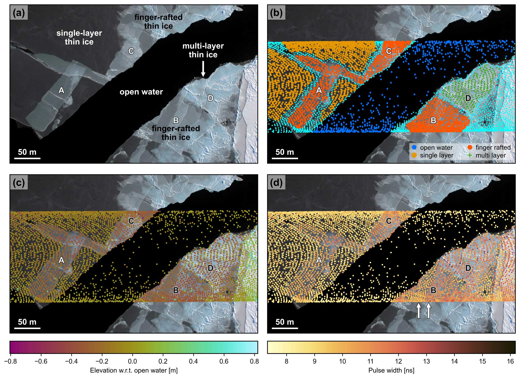
Figure A1Alternative version of Fig. 2 using CVD-friendly color palettes from Crameri (2023). (a) Natural-color DMS single frame of sea ice in the Arctic Ocean north of the Beaufort Sea from 4 May 2016 shown in Fig. 1 (location is indicated by the red outline in Fig. 1). Image spans 500 m × 320 m. (b) Surface classification of individual laser footprints. Laser footprints in cyan were not classified. (c) Elevation in m w.r.t. open water calculated using data from the Level 1B airborne lidar product (ILATM1B). (d) Pulse width in nanoseconds estimated at 35 % of the maximum amplitude above the signal baseline. A pronounced change in pulse width related to the transition from single-layer to finger-rafted ice can be observed in area B (marked by two arrows in Fig. 2d).
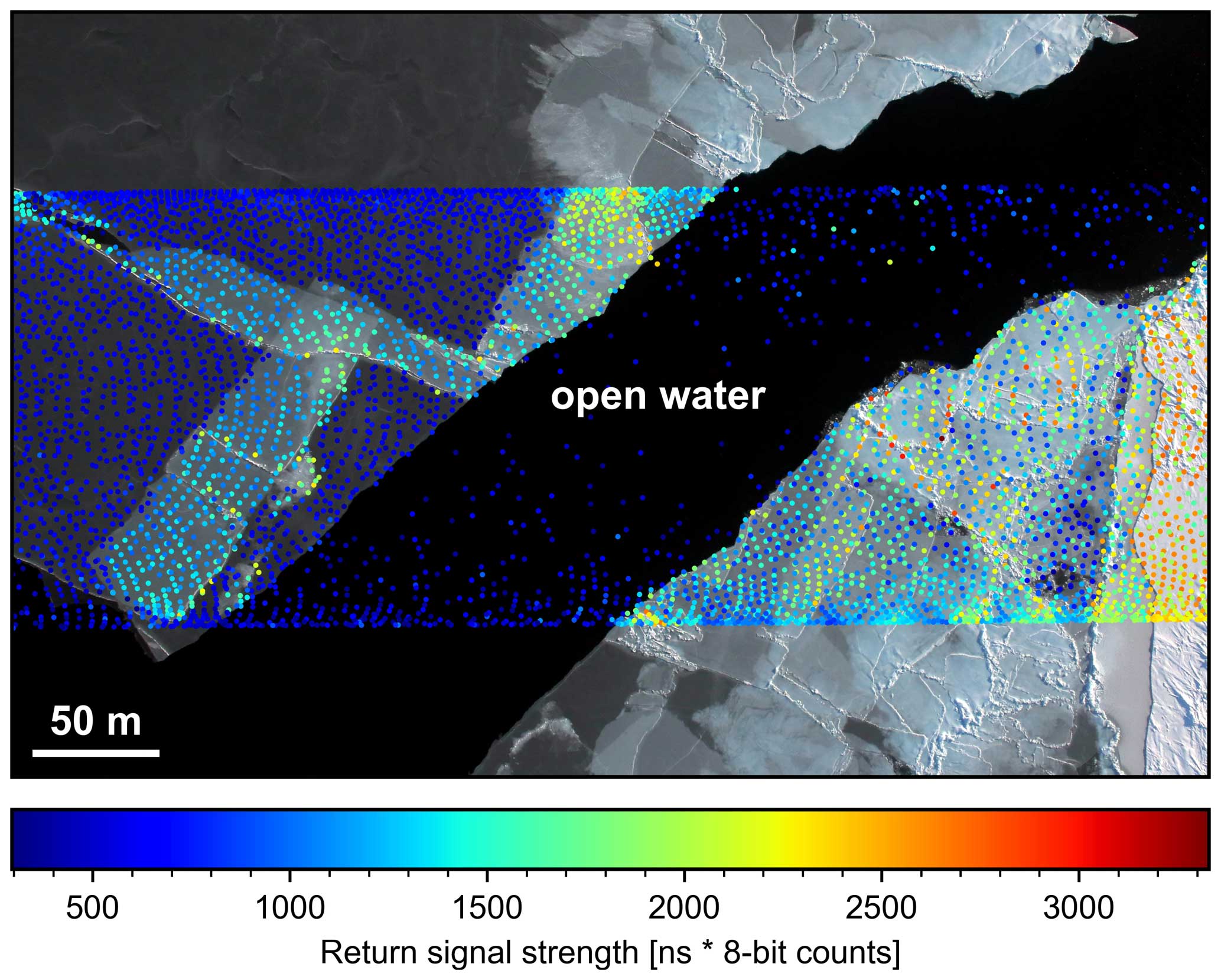
Figure A2Return signal strength of the area shown in Fig. 2. The return signal strength is estimated from trapezoidal numerical integration using the part of the waveforms above 35 % of the maximum amplitude of the pulse above the signal baseline. The 35 % threshold for computing the approximate integral is consistent with the amplitude threshold used for range determination for this campaign.
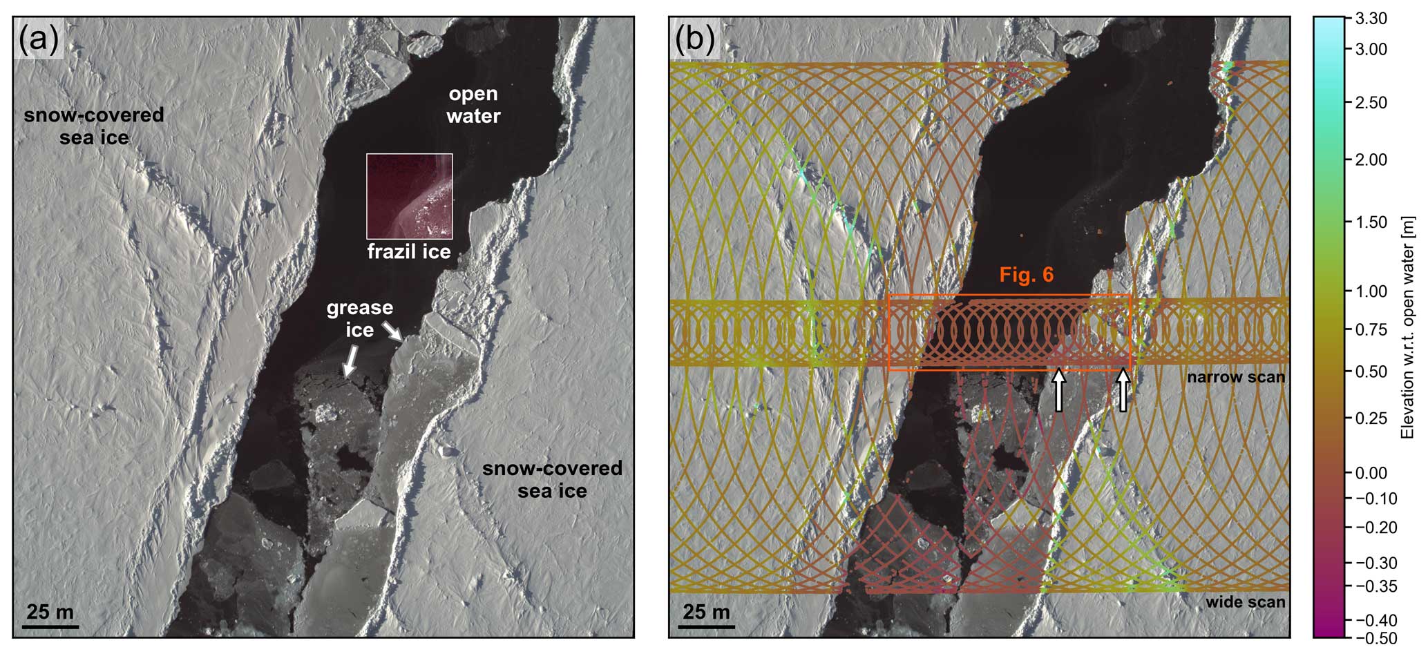
Figure A3Alternative version of Fig. 5 using CVD-friendly color palettes from Crameri (2023). (a) Natural-color CAMBOT image of sea ice 250 km north of the Svalbard archipelago in the Arctic Ocean from 20 April 2019 (image center location N, E). Image spans 290 m × 290 m. The image contrast in a 40 m × 40 m window (white frame) was enhanced to make the frazil ice in the upper few centimeters of the water visible. (b) ATM wide-scan (ATM6A-T6) and narrow-scan (ATM6D-T7) elevations w.r.t. open water. The location of the elevation profile shown in Fig. 6 is indicated by the red outline. The two arrows indicate locations of pulse broadening along the profile that is discussed in Fig. 6.
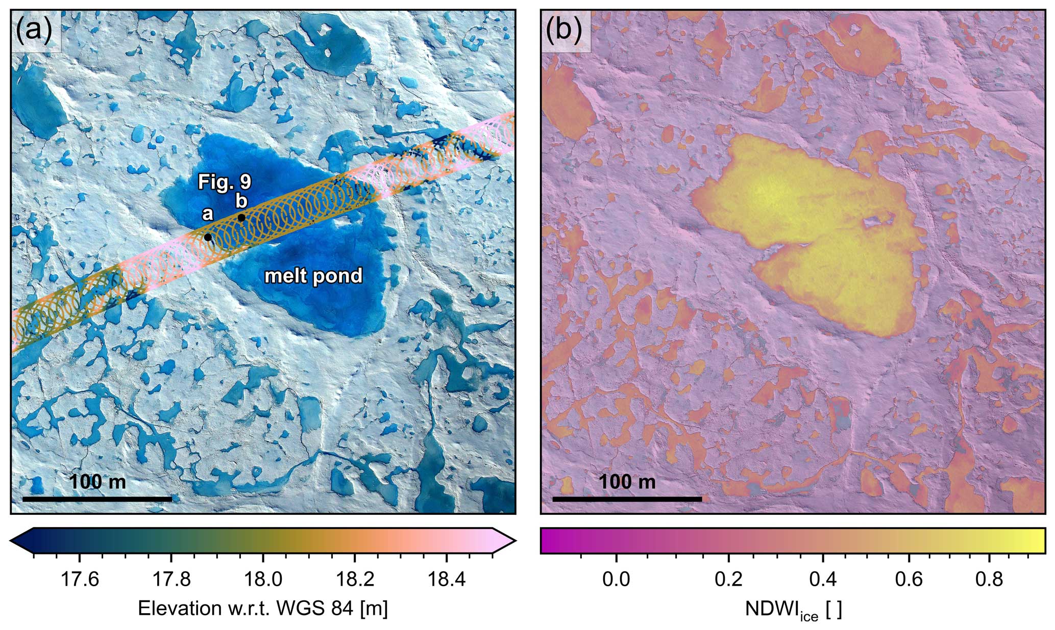
Figure A4Alternative version of Fig. 8 using CVD-friendly color palettes from Crameri (2023). (a) Natural-color (RGB) imagery with ATM6AT5 lidar elevation measurements from 25 July 2017 in the Lincoln Sea north of Ellesmere Island showing melt ponds, meltwater channels, and snow-covered sea ice. Locations of example waveforms shown in Fig. 9 are marked by black dots. (b) NDWIice highlighting melt ponds and liquid water on the surface.
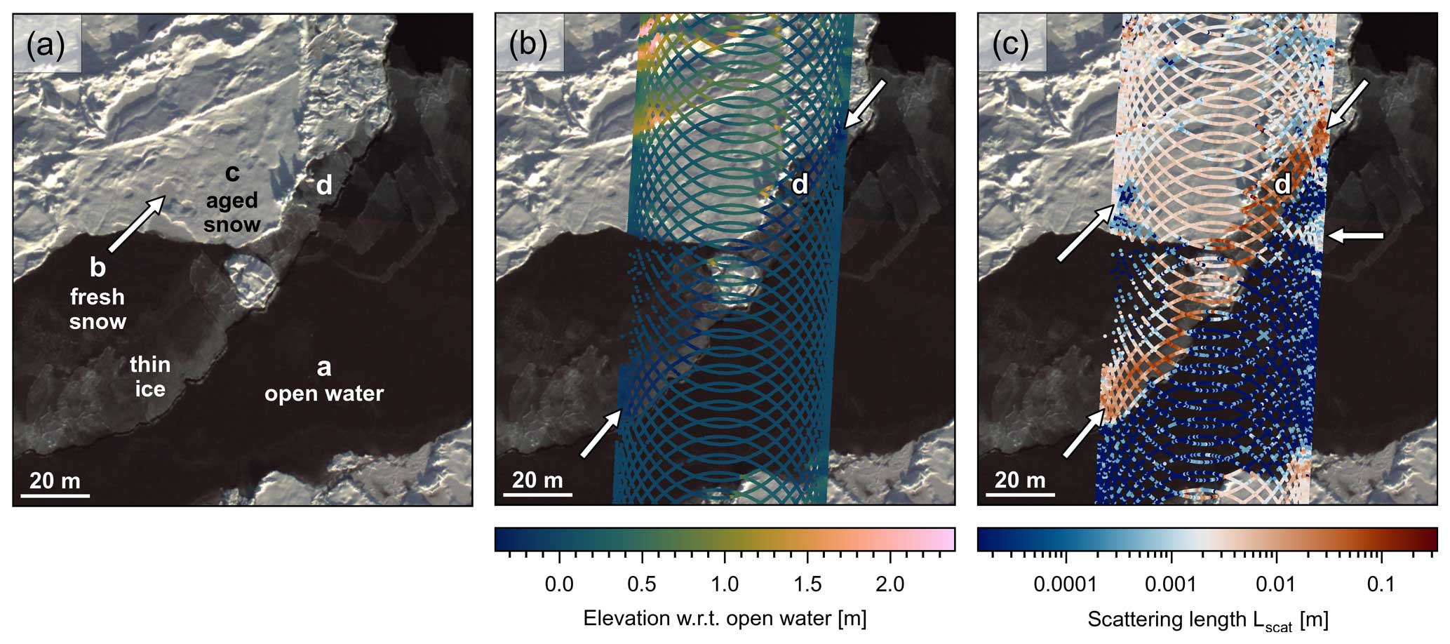
Figure A5Alternative version of Fig. 10 using CVD-friendly color palettes from Crameri (2023). (a) Natural-color CAMBOT image of sea ice in the Wandel Sea from 9 September 2019 (image center location is N, W). Image spans 140 m × 150 m with a pixel resolution of 20 cm × 20 cm due to higher-than-normal flight elevation. Labels in lower case letters in panels (a) to (c) are as follows: a is open water, b is fresh snow, c is aged snow, and d is thin ice, and these indicate locations of lidar and model waveforms shown in Fig. 11. (b) ATM narrow-scan (ATM6D-T7) elevations w.r.t. open water. (c) Modeled scattering length (Lscat) showing longer scattering lengths over thin ice. A band of thin ice elevations below the water surface is marked by arrows in panel (b) and shows longer scattering lengths (marked by arrows). The location of the image frame is shown in Fig. 13.
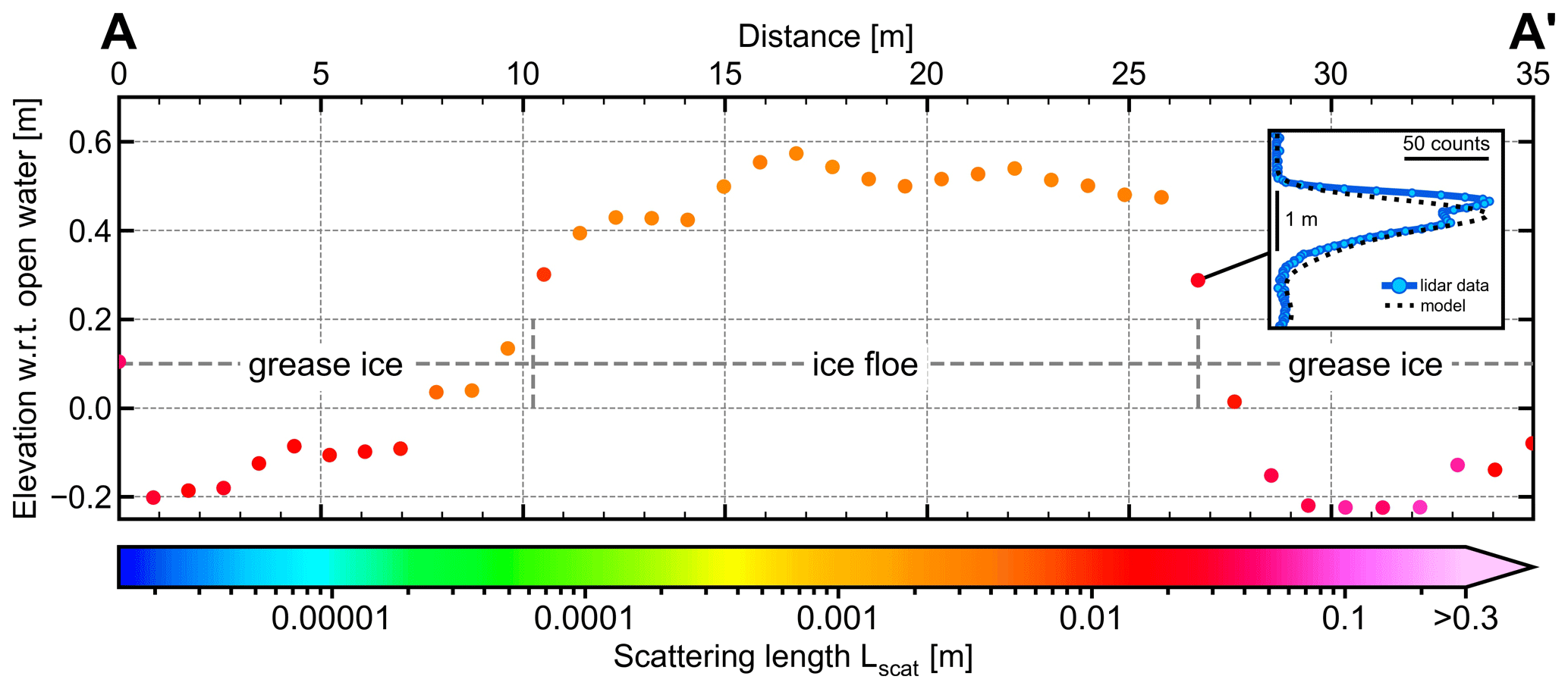
Figure A6Elevation profile along a lidar scan line from A to A'. For the location, see Fig. 12a. Color indicates modeled scattering length Lscat in meters. The profile goes from grease ice over a small snow-covered ice floe and ends over grease ice. Elevations over grease ice are negative (w.r.t. open water) and coincide with longer scattering length indicating differential penetration. An example waveform and model fit at 26.5 m over the steep edge of the ice floe consists of two distinct peaks, indicating a complex surface within the laser footprint. The location of this waveform is marked by an arrow in the inset map in Fig. 12a. The associated pulse broadening here is not related to differential penetration but surface roughness. The surface slope of the ice floe suggests that the surface with the lidar footprints may also be tilted, but the slope does not seem to impact pulse width and therefore model scattering length.
MATLAB® functions used for ATM data and analyzing waveforms are available at https://doi.org/10.5281/zenodo.6341229 (Studinger, 2022) and https://github.com/mstudinger/ATM-Bathymetry-Toolkit (last access: March 2024). A Jupyter notebook demonstrating a Python™ implementation of the ATM centroid tracker is available at https://github.com/mstudinger/ATM-Centroid-Tracker (last access: 29 May 2024) and https://doi.org/10.5281/zenodo.10676624 (Studinger, 2024).
All data used in this study are freely available. ATM airborne data collected for Operation IceBridge are available at the National Snow and Ice Data Center (NSIDC) at https://nsidc.org/icebridge/portal (last access: July 2023). Individual data products from this collection and their access are listed in the references. The ATM ground test data, including lidar waveforms, true ranges, and MATLAB® code for reading ground test data for ATM campaigns with airborne waveform data products at NSIDC are available at https://doi.org/10.5281/zenodo.7225937 (Studinger et al., 2022a).
Airborne data from the Arctic 2016 campaign were collected prior to waveform data products delivered to NSIDC and are available at https://doi.org/10.5281/zenodo.8189441 (Studinger et al., 2023). Data for the Arctic 2016 campaign also include the ground calibration data and a link to MATLAB® functions for reading the ground data.
The ATLAS/ICESat-2 L3A Sea Ice Freeboard (ATL10), Version 6 data are available from NSDIC at https://doi.org/10.5067/ATLAS/ATL10.006 (Kwok et al., 2023).
The Aqua true-color image mosaic of corrected reflectance used as background in Fig. 13 is available from NASA Worldview Earthdata at https://worldview.earthdata.nasa.gov (last access: 6 April 2024) (NASA Worldview Earthdata, 2019).
MS led the analysis of the lidar and optical imagery, integration of results, and preparation of the manuscript. BES and TS developed the scattering model and contributed to writing the modeling section. NK analyzed the ICESat-2 ATL10 data and contributed to writing Sect. 7. All authors helped develop the study and methods, interpret the analysis, and commented on the manuscript.
At least one of the (co-)authors is a member of the editorial board of The Cryosphere. The peer-review process was guided by an independent editor, and the authors also have no other competing interests to declare.
Publisher's note: Copernicus Publications remains neutral with regard to jurisdictional claims made in the text, published maps, institutional affiliations, or any other geographical representation in this paper. While Copernicus Publications makes every effort to include appropriate place names, the final responsibility lies with the authors.
The work presented in this paper was made possible by the combined efforts of all ATM team members developing instruments and data products and collecting data over the course of many decades. Serdar Manizade, Matt Linkswiler, Jim Yungel, and C. Wayne Wright are thanked in particular for discussions about lidar systems and data products. Jeremy Harbeck and Al Ivanoff are thanked for discussions about surface classification and lead detection. Marco Bagnardi is thanked for discussions throughout the course of this project. We thank the Operation IceBridge flight crews for the many years of data collection. We thank the editor Huw Horgan and two anonymous reviewers for their thorough reviews and thoughtful comments that helped improve the manuscript.
This work was funded by NASA's Internal Scientist Funding Model, the Airborne Science Program, and the Cryospheric Sciences Program.
This paper was edited by Huw Horgan and reviewed by two anonymous referees.
Abdalati, W., Zwally, H. J., Bindschadler, R., Csatho, B., Farrell, S. L., Fricker, H. A., Harding, D., Kwok, R., Lefsky, M., Markus, T., Marshak, A., Neumann, T., Palm, S., Schutz, B., Smith, B., Spinhirne, J., and Webb, C.: The ICESat-2 Laser Altimetry Mission, P. IEEE, 98, 735–751, https://doi.org/10.1109/jproc.2009.2034765, 2010.
Brenner, A. C., Zwally, H. J., Bentley, C. R., Csathó, B. M., Harding, D. J., Hofton, M. A., Minster, J.-B., Roberts, L., Saba, J. L., Thomas, R. H., and Yi, D.: The Algorithm Theoretical Basis Document for the Derivation of Range and Range Distributions from Laser Pulse Waveform Analysis for Surface Elevations, Roughness, Slope, and Vegetation Heights, https://ntrs.nasa.gov/citations/20120016646 (last access: 29 May 2024), 2012.
Buckley, E. M., Farrell, S. L., Duncan, K., Connor, L. N., Kuhn, J. M., and Dominguez, R. T.: Classification of Sea Ice Summer Melt Features in High-Resolution IceBridge Imagery, J. Geophys. Res.-Oceans, 125, e2019JC015738, https://doi.org/10.1029/2019JC015738, 2020.
Crameri, F.: Scientific colour maps (8.0.1), Zenodo [code], https://doi.org/10.5281/zenodo.8409685, 2023.
Dominguez, R. T.: IceBridge DMS L1B Geolocated and Orthorectified Images, Version 1 (IODMS1B), NASA National Snow and Ice Data Center Distributed Active Archive Center [data set], https://doi.org/10.5067/OZ6VNOPMPRJ0, 2010.
Flanner, M. G., Liu, X., Zhou, C., Penner, J. E., and Jiao, C.: Enhanced solar energy absorption by internally-mixed black carbon in snow grains, Atmos. Chem. Phys., 12, 4699–4721, https://doi.org/10.5194/acp-12-4699-2012, 2012.
Fox-Kemper, B., Hewitt, H. T., Xiao, C., Aðalgeirsdóttir, G., Drijfhout, S. S., Edwards, T. L., Golledge, N. R., Hemer, M., Kopp, R. E., Krinner, G., Mix, A., Notz, D., Nowicki, S., Nurhati, I. S., Ruiz, L., Sallée, J.-B., Slangen, A. B. A., and Yu, Y.: Ocean, Cryosphere and Sea Level Change. In Climate Change 2021: The Physical Science Basis, Contribution of Working Group I to the Sixth Assessment Report of the Intergovernmental Panel on Climate Change, edited by: Masson-Delmotte, V., Zhai, P., Pirani, A., Connors, S. L., Péan, C., Berger, S., Caud, N., Chen, Y., Goldfarb, L., Gomis, M. I., Huang, M., Leitzell, K., Lonnoy, E., Matthews, J. B. R., Maycock, T. K., Waterfield, T., Yelekçi, O., Yu, R., and Zhou, B., Cambridge University Press, Cambridge, United Kingdom and New York, NY, USA, 1211–1362, https://doi.org/10.1017/9781009157896.011, 2021.
Gardner, A. S. and Sharp, M. J.: A review of snow and ice albedo and the development of a new physically based broadband albedo parameterization, J. Geophys. Res.-Earth, 115, 2009JF001444, https://doi.org/10.1029/2009JF001444, 2010.
Harding, D., Dabney, P., Valett, S., Yu, A., Vasilyev, A., and Kelly, A.: Airborne polarimetric, two-color laser altimeter measurements of lake ice cover: A pathfinder for NASA's ICESat-2 spaceflight mission, 2011 IEEE International Geoscience and Remote Sensing Symposium, 24–29 July 2011, Vancouver, Canada, 3598–3601, https://doi.org/10.1109/IGARSS.2011.6050002, 2011.
Krabill, W., Abdalati, W., Frederick, E., Manizade, S., Martin, C., Sonntag, J., Swift, R., Thomas, R., Wright, W., and Yungel, J.: Greenland ice sheet: High-elevation balance and peripheral thinning, Science, 289, 428–430, https://doi.org/10.1126/science.289.5478.428, 2000.
Krabill, W. B., Abdalati, W., Frederick, E. B., Manizade, S. S., Martin, C. F., Sonntag, J. G., Swift, R. N., Thomas, R. H., and Yungel, J. G.: Aircraft laser altimetry measurement of elevation changes of the greenland ice sheet: technique and accuracy assessment, J. Geodyn., 34, 357–376, https://doi.org/10.1016/s0264-3707(02)00040-6, 2002.
Kurtz, N. T. and Markus, T.: Satellite observations of Antarctic sea ice thickness and volume, J. Geophys. Res.-Oceans, 117, 2012JC008141, https://doi.org/10.1029/2012JC008141, 2012.
Kurtz, N. T., Farrell, S. L., Studinger, M., Galin, N., Harbeck, J. P., Lindsay, R., Onana, V. D., Panzer, B., and Sonntag, J. G.: Sea ice thickness, freeboard, and snow depth products from Operation IceBridge airborne data, The Cryosphere, 7, 1035–1056, https://doi.org/10.5194/tc-7-1035-2013, 2013.
Kwok, R. and Cunningham, G. F.: ICESat over Arctic sea ice: Estimation of snow depth and ice thickness, J. Geophys. Res.-Oceans, 113, 2008JC004753, https://doi.org/10.1029/2008JC004753, 2008.
Kwok, R. and Kacimi, S.: Three years of sea ice freeboard, snow depth, and ice thickness of the Weddell Sea from Operation IceBridge and CryoSat-2, The Cryosphere, 12, 2789–2801, https://doi.org/10.5194/tc-12-2789-2018, 2018.
Kwok, R., Zwally, H. J., and Yi, D.: ICESat observations of Arctic sea ice: A first look, Geophys. Res. Lett., 31, 2004GL020309, https://doi.org/10.1029/2004GL020309, 2004.
Kwok, R., Cunningham, G. F., Wensnahan, M., Rigor, I., Zwally, H. J., and Yi, D.: Thinning and volume loss of the Arctic Ocean sea ice cover: 2003–2008, J. Geophys. Res.-Oceans, 114, 2009JC005312, https://doi.org/10.1029/2009JC005312, 2009.
Kwok, R., Markus, T., Morison, J., Palm, S. P., Neumann, T. A., Brunt, K. M., Cook, W. B., Hancock, D. W., and Cunningham, G. F.: Profiling Sea Ice with a Multiple Altimeter Beam Experimental Lidar (MABEL), J. Atmos. Ocean. Tech., 31, 1151–1168, https://doi.org/10.1175/jtech-d-13-00120.1, 2014.
Kwok, R., Cunningham, G. F., Hoffmann, J., and Markus, T.: Testing the ice-water discrimination and freeboard retrieval algorithms for the ICESat-2 mission, Remote Sens. Environ., 183, 13–25, https://doi.org/10.1016/j.rse.2016.05.011, 2016.
Kwok, R., Markus, T., Kurtz, N. T., Petty, A. A., Neumann, T. A., Farrell, S. L., Cunningham, G. F., Hancock, D. W., Ivanoff, A., and Wimert, J. T.: Surface Height and Sea Ice Freeboard of the Arctic Ocean From ICESat-2: Characteristics and Early Results, J. Geophys. Res.-Oceans, 124, 6942–6959, https://doi.org/10.1029/2019JC015486, 2019.
Kwok, R., Petty, A. A., Cunningham, G., Markus, T., Hancock, D., Ivanoff, A., Wimert, J., Bagnardi, M., Kurtz, N., and the ICESat-2 Science Team: ATLAS/ICESat-2 L3A Sea Ice Freeboard, Version 6, Boulder, Colorado USA, National Snow and Ice Data Center [data set], https://doi.org/10.5067/ATLAS/ATL10.006, 2023.
MacGregor, J. A., Boisvert, L. N., Medley, B., Petty, A. A., Harbeck, J. P., Bell, R. E., Blair, J. B., Blanchard-Wrigglesworth, E., Buckley, E. M., Christoffersen, M. S., Cochran, J. R., Csathó, B. M., De Marco, E. L., Dominguez, R. T., Fahnestock, M. A., Farrell, S. L., Gogineni, S. P., Greenbaum, J. S., Hansen, C. M., Hofton, M. A., Holt, J. W., Jezek, K. C., Koenig, L. S., Kurtz, N. T., Kwok, R., Larsen, C. F., Leuschen, C. J., Locke, C. D., Manizade, S. S., Martin, S., Neumann, T. A., Nowicki, S. M. J., Paden, J. D., Richter-Menge, J. A., Rignot, E. J., Rodríguez-Morales, F., Siegfried, M. R., Smith, B. E., Sonntag, J. G., Studinger, M., Tinto, K. J., Truffer, M., Wagner, T. P., Woods, J. E., Young, D. A., and Yungel, J. K.: The Scientific Legacy of NASA's Operation IceBridge, Rev. Geophys., 59, e2020RG000712, https://doi.org/10.1029/2020RG000712, 2021.
Magruder, L., Brunt, K., and Alonzo, M.: Early ICESat-2 on-orbit Geolocation Validation Using Ground-Based Corner Cube Retro-Reflectors, Remote Sens.-Basel, 12, 3653, https://doi.org/10.3390/rs12213653, 2020.
Markus, T., Neumann, T., Martino, A., Abdalati, W., Brunt, K., Csatho, B., Farrell, S., Fricker, H., Gardner, A., Harding, D., Jasinski, M., Kwok, R., Magruder, L., Lubin, D., Luthcke, S., Morison, J., Nelson, R., Neuenschwander, A., Palm, S., Popescu, S., Shum, C. K., Schutz, B. E., Smith, B., Yang, Y., and Zwally, J.: The Ice, Cloud, and land Elevation Satellite-2 (ICESat-2): Science requirements, concept, and implementation, Remote Sens. Environ., 190, 260–273, https://doi.org/10.1016/j.rse.2016.12.029, 2017.
Massom, R. A., Eicken, H., Hass, C., Jeffries, M. O., Drinkwater, M. R., Sturm, M., Worby, A. P., Wu, X., Lytle, V. I., Ushio, S., Morris, K., Reid, P. A., Warren, S. G., and Allison, I.: Snow on Antarctic sea ice, Rev. Geophys., 39, 413–445, https://doi.org/10.1029/2000RG000085, 2001.
NASA Worldview Earthdata: Aqua MODIS Corrected Reflectance (True Color), NASA [data set], https://worldview.earthdata.nasa.gov (last access: 6 April 2023), 2019.
Naumann, A. K., Notz, D., Håvik, L., and Sirevaag, A.: Laboratory study of initial sea-ice growth: properties of grease ice and nilas, The Cryosphere, 6, 729–741, https://doi.org/10.5194/tc-6-729-2012, 2012.
Onana, V.-D.-P., Kurtz, N. T., Farrell, S. L., Koenig, L. S., Studinger, M., and Harbeck, J. P.: A Sea-Ice Lead Detection Algorithm for Use With High-Resolution Airborne Visible Imagery, IEEE T. Geosci. Remote, 51, 38–56, https://doi.org/10.1109/tgrs.2012.2202666, 2013.
Ricker, R., Hendricks, S., Helm, V., Skourup, H., and Davidson, M.: Sensitivity of CryoSat-2 Arctic sea-ice freeboard and thickness on radar-waveform interpretation, The Cryosphere, 8, 1607–1622, https://doi.org/10.5194/tc-8-1607-2014, 2014.
Smith, B., Fricker, H. A., Gardner, A. S., Medley, B., Nilsson, J., Paolo, F. S., Holschuh, N., Adusumilli, S., Brunt, K., Csatho, B., Harbeck, K., Markus, T., Neumann, T., Siegfried, M. R., and Zwally, H. J.: Pervasive ice sheet mass loss reflects competing ocean and atmosphere processes, Science, 368, 1239–1242, https://doi.org/10.1126/science.aaz5845, 2020.
Smith, B., Studinger, M., Sutterley, T., Fair, Z., and Neumann, T.: Understanding biases in ICESat-2 data due to subsurface scattering using Airborne Topographic Mapper waveform data, The Cryosphere Discuss. [preprint], https://doi.org/10.5194/tc-2023-147, in review, 2023.
Smith, B. E., Gardner, A., Schneider, A., and Flanner, M.: Modeling biases in laser-altimetry measurements caused by scattering of green light in snow, Remote Sens. Environ., 215, 398–410, https://doi.org/10.1016/j.rse.2018.06.012, 2018.
Studinger, M.: IceBridge ATM L1B Elevation and Return Strength, Version 2 (ILATM1B), NASA National Snow and Ice Data Center Distributed Active Archive Center [data set], https://doi.org/10.5067/19SIM5TXKPGT, 2013.
Studinger, M.: IceBridge Narrow Swath ATM L1B Elevation and Return Strength, Version 2 (ILNSA1B), NASA National Snow and Ice Data Center Distributed Active Archive Center [data set], https://doi.org/10.5067/CXEQS8KVIXEI, 2014.
Studinger, M.: IceBridge ATM L1B Elevation and Return Strength with Waveforms, Version 1 (ILATMW1B), NASA National Snow and Ice Data Center Distributed Active Archive Center [data set], https://doi.org/10.5067/EZQ5U3R3XWBS, 2018a.
Studinger, M.: IceBridge Narrow Swath ATM L1B Elevation and Return Strength with Waveforms, Version 1 (ILNSAW1B), NASA National Snow and Ice Data Center Distributed Active Archive Center [data set], https://doi.org/10.5067/V25X7LHDPMZY, 2018b.
Studinger, M.: Airborne Topographic Mapper (ATM) Bathymetry Toolkit (1.0), Zenodo [code], https://doi.org/10.5281/zenodo.6341229, 2022.
Studinger, M.: ATM Centroid Tracker (1.0.1), Zenodo [code], https://doi.org/10.5281/zenodo.10676624, 2024.
Studinger, M. and Harbeck, J.: IceBridge CAMBOT L1B Geolocated Images, Version 2 (IOCAM1B), NASA National Snow and Ice Data Center Distributed Active Archive Center [data set], https://doi.org/10.5067/B0HL940D452L, 2019.
Studinger, M., Medley, B. C., Brunt, K. M., Casey, K. A., Kurtz, N. T., Manizade, S. S., Neumann, T. A., and Overly, T. B.: Temporal and spatial variability in surface roughness and accumulation rate around 88° S from repeat airborne geophysical surveys, The Cryosphere, 14, 3287–3308, https://doi.org/10.5194/tc-14-3287-2020, 2020.
Studinger, M., Linkswiler, M. A., Manizade, S. S., and Yungel, J. K.: NASA's Airborne Topographic Mapper (ATM) ground calibration data for waveform data products, Zenodo [data set], https://doi.org/10.5281/zenodo.7225936, 2022a.
Studinger, M., Manizade, S. S., Linkswiler, M. A., and Yungel, J. K.: High-resolution imaging of supraglacial hydrological features on the Greenland Ice Sheet with NASA's Airborne Topographic Mapper (ATM) instrument suite, The Cryosphere, 16, 3649–3668, https://doi.org/10.5194/tc-16-3649-2022, 2022b.
Studinger, M., Manizade, S., Linkswiler, M. A., and Yungel, J. K.: NASA's Airborne Topographic Mapper (ATM) airborne waveform and ground calibration data for the Arctic Spring campaign 2016 (1), Zenodo [data set], https://doi.org/10.5281/zenodo.8189441, 2023.
Thomas, R. H. and PARCA Investigators: Program for arctic regional climate assessment (PARCA): Goals, key findings, and future directions, J. Geophys. Res.-Atmos., 106, 33691–33705, https://doi.org/10.1029/2001jd900042, 2001.
Webster, M., Gerland, S., Holland, M., Hunke, E., Kwok, R., Lecomte, O., Massom, R., Perovich, D., and Sturm, M.: Snow in the changing sea-ice systems, Nat. Clim. Change, 8, 946–953, https://doi.org/10.1038/s41558-018-0286-7, 2018.
World Meteorological Organization: WMO Sea-Ice Nomenclature, Volume I – Terminology and codes, https://library.wmo.int/index.php?lvl=notice_display&id=6772#.Y-BHJa3MImA (last access: 29 May 2024), World Meteorological Organization, 2014.
Wright, C. W., Kranenburg, C., Battista, T. A., and Parrish, C.: Depth Calibration and Validation of the Experimental Advanced Airborne Research Lidar, EAARL-B, J. Coastal Res., 76, 4–17, 2016.
Wright, N. C. and Polashenski, C. M.: Open-source algorithm for detecting sea ice surface features in high-resolution optical imagery, The Cryosphere, 12, 1307–1329, https://doi.org/10.5194/tc-12-1307-2018, 2018.
Xie, H., Tang, H., Jin, Y., Li, B., Zhang, Z., Liu, S., and Tong, X.: An Improved Surface Slope Estimation Model Using Space-Borne Laser Altimetric Waveform Data Over the Antarctic Ice Sheet, IEEE Geosci. Remote S., 19, 1–5, https://doi.org/10.1109/LGRS.2021.3124224, 2022.
Yang, K. and Smith, L. C.: Supraglacial Streams on the Greenland Ice Sheet Delineated From Combined Spectral–Shape Information in High-Resolution Satellite Imagery, IEEE Geosci. Remote S., 10, 801–805, https://doi.org/10.1109/LGRS.2012.2224316, 2013.
Zatko, M. C. and Warren, S. G.: East Antarctic sea ice in spring: spectral albedo of snow, nilas, frost flowers and slush, and light-absorbing impurities in snow, Ann. Glaciol., 56, 53–64, https://doi.org/10.3189/2015AoG69A574, 2015.
Zwally, H. J., Schutz, B., Abdalati, W., Abshire, J., Bentley, C., Brenner, A., Bufton, J., Dezio, J., Hancock, D., Harding, D., Herring, T., Minster, B., Quinn, K., Palm, S., Spinhirne, J., and Thomas, R.: ICESat's laser measurements of polar ice, atmosphere, ocean, and land, J. Geodyn., 34, 405–445, https://doi.org/10.1016/s0264-3707(02)00042-x, 2002.
- Abstract
- Introduction
- Instruments and data sets
- Methods
- Results: observations of differential penetration over sea ice
- Modeling subsurface volume scattering
- Prevalence of anomalous elevations caused by differential penetration
- Discussion of the results in a broader context
- Conclusions
- Appendix A
- Code availability
- Data availability
- Author contributions
- Competing interests
- Disclaimer
- Acknowledgements
- Financial support
- Review statement
- References