the Creative Commons Attribution 4.0 License.
the Creative Commons Attribution 4.0 License.
 | 29 May 2024
Brief communication: Testing a portable Bullard-type temperature lance confirms highly spatially heterogeneous sediment temperatures under shallow bodies of water in the Arctic
Frederieke Miesner
William Lambert Cable
Pier Paul Overduin
Julia Boike
The thermal regime in the sediment column below shallow bodies of water in Arctic permafrost controls benthic habitats and permafrost stability. We present a robust, portable device that measures detailed temperature–depth profiles of the near-surface sediments in less than 1 h. Test campaigns in the Canadian Arctic and on Svalbard have demonstrated its utility in a range of environments during winter and summer. Measured temperatures were spatially heterogeneous, even within single bodies of water. We observed the broadest temperature range in water less than 1 m deep, a zone that is not captured by single measurements in deeper water.
- Article
(2330 KB) - Full-text XML
- BibTeX
- EndNote


Approximately 6 % of land in the Arctic is covered with lakes, with small lakes (smaller than 0.01 km2) making up about 32 % of the lakes (Paltan et al., 2015). Bodies of water in the permafrost region in the Arctic cause thermal disturbances in comparison to the surrounding ground (i.e., Boike et al., 2015; Jorgenson et al., 2010; Burn, 2002). As the mean annual water temperature is usually above 0 °C even if the mean annual air temperature is below 0 °C, unfrozen zones within the permafrost, called taliks, can form below the bodies of water. However, in areas with water shallower than the maximum ice thickness, the presence of bottom-fast ice can decrease the mean annual bed temperature and significantly slows the thawing of or even refreezes the lake or seabed in winter (Roy-Leveillee and Burn, 2017; Arp et al., 2016). In the transition zone between floating and bottom-fast ice, small changes in water level have the potential to drastically alter the sub-bed thermal regime between permafrost thawing and permafrost forming.
Among other factors, higher temperatures can render taliks hot spots of methane emission (Abnizova et al., 2012). A better understanding of the spatial variability with temperature measurements in a fine mesh can therefore help better constrain the emission potential of shallow Arctic bodies of water. However, such distributed measurements of sediment temperatures are scarce. Temperature lances were designed for measuring in situ temperatures and even sediment thermal properties (Lister, 1970; Hyndman et al., 1979; Sclater et al., 1969; Christoffel and Calheam, 1969), but their use in the Arctic, and especially under small lakes, requires portability and robust design. Due to ice cover dynamics and ice movement during the melt period, monitoring with permanently installed devices is generally not feasible in the Arctic. Commonly used in offshore marine environments are heat flow probes of the Bullard type (the sensor string is directly attached to the logger and pushed into the sediment; Christoffel and Calheam, 1969; Lindqvist, 1984), the Lister or violin-bow type (the sensor string is attached like a violin bow to a solid strength member that is lowered into the sediment; Lister, 1970; Hyndman et al., 1979), or the Ewing type (outrigger fins with sensors are attached to a piston or gravity corer; Riedel et al., 2015). These devices are heavy and require larger ships for deployment (Hornbach et al., 2021), and surveys are typically focused more on the thermal properties and the geothermal heat flow than on the temperature field alone (Dziadek et al., 2021). Furthermore, they are not useful to small lakes or the shallow waters of the nearshore zone due to their weight and unwieldy design. Smaller lances are being used to monitor sediment temperatures in permafrost areas (Dafflon et al., 2022) but are not suitable for submergence. Published temperature–depth profiles in the nearshore zone and under shallow lakes were recorded with temperature chains in boreholes (i.e., Solomon et al., 2008; Brown et al., 1964; Burn, 2002). Although these yield good-quality data to potentially great depths, single-location temperature–depth profiles hold no information about the spatial variability in temperatures. In addition, although boreholes afford us a chance to repeat measurements or even measure a continuous time series, in aquatic environments, they are often disturbed or destroyed by ice movement. Lindqvist (1984) used a Bullard-type probe to monitor lake bed temperatures in northern Sweden, but the device was also not portable enough to make spatially distributed measurements. An even smaller probe was developed and used to monitor temperatures in the upper 40 cm of the tidal plains in the German Wadden Sea (Onken et al., 2010), where deployment is easy during low tide.
We therefore suggest that using a lightweight robust device to quickly measure temperature profiles under shallow lakes in the Arctic could fill a knowledge gap addressing spatial variability in sediment temperatures in shallow water.
Here, we present a newly developed temperature lance and its applicability in a number of Arctic environments, providing a detailed technical description of its design, the construction, and the intended modes of operation, as well as the post-processing of the data before showcasing collected data sets to demonstrate the device's utility.
2.1 Technical description
The temperature lance is built from high-grade stainless steel, which ensures its durability and resistance to corrosion. The lance is 1.5 m long and 20 mm in diameter. The sensor string comprises 15 digital nodes with 2 temperature sensors each, resulting in 30 temperature sensors with a 5 cm spacing (see Fig. 1). The temperature nodes are soldered together and thus connected end to end, forming a common communication and power bus. The digital temperature sensor used is a TSYS01-1 (G-NICO-023; TE Connectivity) with an accuracy of ±0.1 °C and resolution of 0.01 °C.
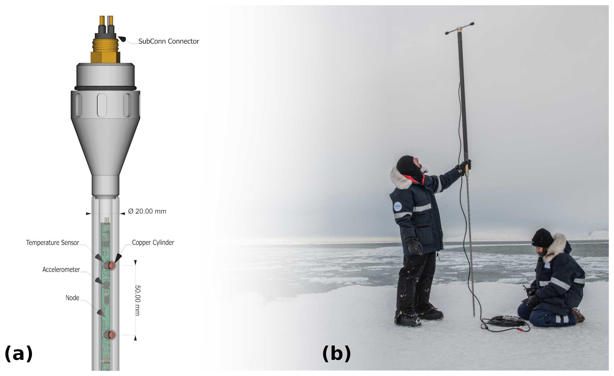
Figure 1(a) A technical drawing of the head of the temperature lance. A string of 15 nodes is housed inside the lance, with copper cylinders protruding the stainless steel body, coupling the temperature sensors with their surroundings. Two temperature sensors are mounted on each node; on two nodes (at the top and in the middle of the lance), an additional accelerometer is mounted. (b) The temperature lance assembled with one carbon fiber extension for deployment in up to 1.5 m deep water and connected by a waterproof cable to the logger unit.
To shorten equilibration time with the surrounding sediment, small copper cylinders couple the temperature sensors through the body of the lance with the outside environment (see Fig. 1). The thermal conductivity of the copper (κcopper≈360 W m−1 K−1) is approximately 20 times higher than that of the stainless steel body (κsteel≈18 W m−1 K−1), ensuring that the vertical heat conduction is negligible compared to the horizontal component.
Digital three-axis accelerometers (ADXL345; Analog Devices) are installed on two of the nodes, at the top and in the middle of the lance. The accelerometers measure the static acceleration of gravity from which inclination can be calculated. The high resolution of the sensor allows for measurements of inclination changes of less than 1.0°. This information can be used during deployment to assess departure from the vertical and in post-processing to correct sensor depths.
Finally, the lance body is filled with a urethane potting compound, which also has a lower thermal conductivity (κurethane≈0.35 W m−1 K−1) than the copper pieces and stainless steel body, to protect the electronics.
Measurements are conducted with an Arduino-based logger containing a GNSS module to obtain accurate recordings of date, time, and position for each measurement. Communication with the temperature nodes is realized via the 1-Wire protocol (Maxim Integrated, Analog Devices), which allows for cable lengths of over 100 m. The logger unit and a battery pack (four AA batteries) are housed in a small waterproof case, attached to the device with a cable and a SubConn connector, and operated using four buttons. In Fig. 1b, the logger unit is lying on the ground in the cable coil. The logger records the temperature measurements onto a micro SD card. During an active measurement, the logger unit indicates whether the most recent two measurements at each sensor have changed more than a certain threshold. We suggest a threshold of 0.02 °C and a measurement interval of 30 s, but both can be adjusted. The GNSS receiver is located in the logger unit, and the position is written to the data file only once at the beginning of each measurement – i.e., the logger unit must be located at the measurement location when starting a measurement.
2.2 Deployment options
The temperature lance is inserted into the sediment, usually by hand, and then left undisturbed for several minutes until the temperatures of the sensors are in equilibrium with the surrounding sediment – i.e., until the maximum temperature-change threshold condition is satisfied. The resistance to insertion and the equilibration time depend largely on the sediment composition. The device is robust enough to allow hammered insertion if needed. The options for deployment include insertion through a hole in ice cover, from vessels at the water surface (may require anchoring or stabilization), or from a wading position in shallow water. Deployment is not restricted to aquatic environments – i.e., temperature measurements can be made in the active layer and in taliks or any material loose enough to permit insertion. Lightweight hollow carbon fiber extensions are threaded onto the temperature lance during the deployment in deeper water.
2.3 Post-processing of the data
The calibration of each temperature sensor was checked at 0 °C in an ice bath (Wise, 1988), and the offset from 0 °C was measured before the assembly of the lance. Measured temperatures are corrected by the logger unit at the time of measurement using these offsets.
As the lance has no pressure sensor, the penetration depth has to be estimated based on additional observations in the field and in the time series of the measurements. We measured the water depth with an independent device and with the lance and the extensions used to obtain the penetration depth in the field. The difference between water and sediment is also visible in the recorded data. With the 5 cm spacing of the temperature sensors, this yields an error of the same amount.
When the device enters the sediment, it has a temperature close to the air or water temperature, which may be several degrees warmer or colder than the sediment, and frictional heat from the penetration of the measurement device heats up the sediment (Carslaw and Jaeger, 1959). Both factors may perturb sediment temperature, meaning that measured sensor temperatures do not reflect the undisturbed in situ sediment temperature. We employ an inversion scheme, following Bullard (1954), Lister (1970), and Hartmann and Villinger (2002), to determine in situ temperatures. For each measurement, we leave the lance undisturbed in the sediment until the threshold of 0.02 °C between two consecutive measurements is not exceeded for at least four measurements. The time series of temperature measurements is then fit to the theoretical function for temperature decay from a cylindrical source of heat:
where Θ is the temperature over time t, Θ0 is the undisturbed sediment temperature, and δΘ is the disturbance introduced by the temperature lance, with the integral describing the decreasing amplitude of this disturbance with distance to the lance body (Bullard, 1954). The variable is a composite of the thermal properties of the lance body (m=360 W m−1 K−1 being the thermal conductivity and a=0.0095 m the length of the copper pieces) and the sediment (the effective heat capacity, σ, and the density, ρ, measured or estimated at each location), and is a scaled time variable. The function f is integrated over the radial coordinate x (i.e., the distance to the lance body) and is written with the Bessel functions J and Y to be
We use a least-squares algorithm to fit the measured temperatures over time to Eq. (1), with the in situ temperature, Θ0; the introduced disturbance, Θ1; and the thermal properties of the sediment as free variables.
2.4 Study sites
We provide a comprehensive analysis of sediment temperature measurements obtained from various Arctic study sites: (a) the beach zone of Tuktoyaktuk Island in the harbor of Tuktoyaktuk, Northwest Territories (NWT), Canada; (b) a shallow lagoon near Ny-Ålesund, Svalbard; (c) an old river arm in the outer Mackenzie Delta; (d) a small thermokarst lake near the Inuvik–Tuktoyaktuk Highway, NWT, Canada; and (e) the drinking-water reservoir of Ny-Ålesund, Svalbard.
-
Site (a), Tuktoyaktuk Island, is a barrier island in the harbor of the hamlet of Tuktoyaktuk on the Arctic coast in the Northwest Territories, Canada. The coastline has changed dramatically over the last few decades due to coastal erosion, especially in the case of the north-facing shore, which moves slowly southwards at 1–2 m yr−1 (Whalen et al., 2022).
-
Sites (b) and (e) – the lagoon, Brandalaguna, and the drinking-water lake, Tvillingvatnet, near Ny-Ålesund – we accessed by snowmobile in March 2021. The lagoon has a shallow water depth of 1.4 m and brackish water with salinity of around 2–3 psu. At the location where we measured in the drinking-water lake, the water was 4.6 m deep; however, the maximum water depth is greater than that. We carried out the equilibration experiment at the drinking-water lake. Both bodies of water were covered by ≈60 cm thick ice.
-
Site (c), the old river arm in the outer Mackenzie Delta is sometimes called Swiss Cheese Lake, because ebullition, even in winter, maintains holes in the ice cover. The lake is reachable by boat and a 2 km hike or by helicopter in summer or by snowmobile from the ice road in winter.
-
Site (d), the small thermokarst lake, dubbed Lake 3 throughout this paper, is located about 300 m from the Inuvik–Tuktoyaktuk Highway and therefore easily accessible throughout the year.
The device was tested on multiple expeditions in the Arctic in summer and in winter. Operation through a hole in the ice and from a wading position in late summer proved to be executable by a single person. Assistance was useful for applying more weight when pushing the device into the sediment but not strictly necessary. Operating the device from small boats was always a two-person job and was most successful in calm weather without wind and waves.
The visited sites cover freshwater and marine-influenced bodies of water, with sediment grain sizes ranging from fine silty sands to coarse gravel and shallow and swampy, as well as deeper water. In locations with coarser sand and gravel, the sediment insertion depth was sometimes limited to 1 m.
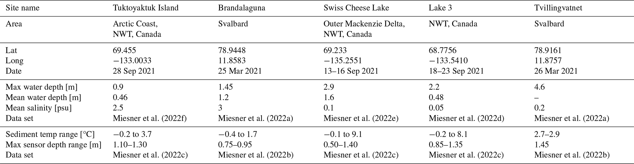
The measured sediment temperature–depth profiles range from nearly isothermal states to temperature gradients of more than 9 K m−1. An overview of the site and measurement characteristics is given in Table 1.
Miesner et al. (2022f)Miesner et al. (2022a)Miesner et al. (2022e)Miesner et al. (2022d)Miesner et al. (2022a)Miesner et al. (2022c)Miesner et al. (2022b)Miesner et al. (2022c)Miesner et al. (2022c)Miesner et al. (2022b)Table 1Summary of the covered sites of investigation. The water parameters were measured with a CastAway-CTD prior to each measurement with the temperature lance. The data sets are individually available via PANGAEA.
3.1 Post-processing of the data
To assess the accuracy of the results of the inversion algorithm, we conducted a 12 h measurement in March 2021 at the drinking-water lake near Ny-Ålesund, Svalbard. The measurement was taken at 4.6 m water depth under floating-ice conditions We assume that there was no diurnal variability in the bottom-water temperature at that water depth so that the mean of the measurements after 12 h reflected the in situ temperature. With this measurement we compared the inversely determined in situ temperatures with the mean over three consecutive measurements and explored how the accuracy changes with time following the beginning of the measurement. Figure 2 shows the maximum absolute error over the whole temperature–depth profile for the mean of three measurements (blue crosses) and the inversely determined results (pink circles). The error in inversely determined temperature–depth profiles was smaller by ≈0.01 °C than for the means for measurement times shorter than 45 min. Both yielded results within the sensor accuracy of 0.01 °C after ≈80 min. For even longer measurement times, the means are more accurate than the inversely determined values.
The time needed to equilibrate to in situ temperatures depends on the thermal properties of the sediment and the initial temperature difference between the temperature lance and the sediment. This assessment of error over time from this one long-term measurement is therefore only qualitative. Using the inversion algorithm improves the accuracy of the results in comparison to taking the mean, at least at shorter measurement periods. The time needed to achieve sensor accuracy, however, cannot be determined universally from this experiment. We recommend recording temperatures while allowing the device to equilibrate with the sediment for at least 30 min.
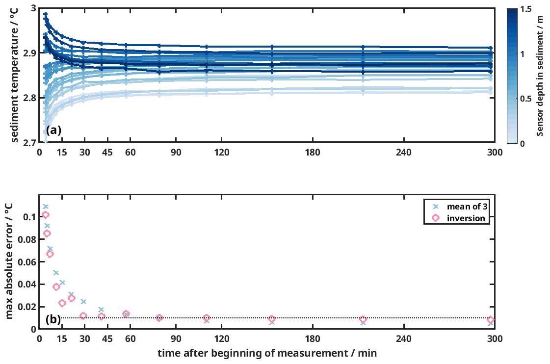
Figure 2(a) Temperature over time after the beginning of the measurement at Tvillingvatnet, Svalbard, for all sensors. The shade of blue indicates the depth of the sensor in the sediment, with lighter shades at the water–sediment interface and darker shades towards a 1.5 m depth in the sediment. Measurements were taken every 60 s. The 14 highlighted points in time (+) indicate the timing of the time periods for which we employed the inversion algorithm. (b) Maximum temperature difference over all sensors for results at different times after the beginning of the measurement. The mean over three measurements after 12 h is assumed to be the in situ temperature – i.e., the reference temperature that the results are compared to. The results from the inversion algorithm are shown in pink circles, the means over three measurements are shown in blue crosses, and the dotted line indicates the sensor accuracy of 0.01 °C.
3.2 Spatial heterogeneity
All temperature–depth profiles for the four locations are shown in Fig. 3.
-
In panel (a), we see the measurements in Tuktoyaktuk harbor taken both south and north of the barrier island. They all show a similar shape, with a temperature increase from the water temperature down to ≈50 cm into the sediment and then a steady decrease below. All profiles suggest a probable upper permafrost boundary in ≤3 m sediment depth. In general, at this site, the deeper the water, the higher the water temperature and the sediment temperature and the greater the assumed depth of the permafrost table.
-
Panel (b) shows the temperature profiles at Brandalaguna, which are the only ones that increased steadily over depth. They are also the only ones measured in late March, when the air temperature was near its annual minimum. The shapes of the temperature–depth profiles are relatively similar to each other, and the measurements are not deep enough to show a potential change in the gradient that would indicate lower temperatures in deeper sediment layers. The water depth shows only little spatial variety, changing only within 20 cm. However, we still observe a temperature difference of >1 °C at the same depths below the sediment–water interface.
-
In panel (c), at Swiss Cheese Lake, the water temperature is relatively stable at 8.5–9 °C. The measurements in water depth >0.9 m show a similar shape and indicate a deep talik. The two shallower measurements, located within 2 m of the lake shore, reach frozen ground at around 1.2 m sediment depth.
-
In panel (d), at Lake 3, we see two clusters of temperature–depth profiles: the first cluster includes measurements in water depths >0.9 m, with water temperatures of ≈6.3 °C. Here, the sediment temperature increases down to ≈60 cm sediment depth and decreases below, pointing to a talik depth of ≥5 m. The second cluster includes measurements in shallower water depth with water temperatures between 1.2 and 4.5 °C, where the temperature–depth profiles show great variability. The four measurements in water depth below 0.3 m reach frozen ground within the upper meter of sediment, while the other measurements point to a talik deeper than the measurements in the deeper parts of the lake would suggest. The temperature–depth profiles are therefore not deep enough that a simple extrapolation could be used to estimate the depth of the talik at this location.
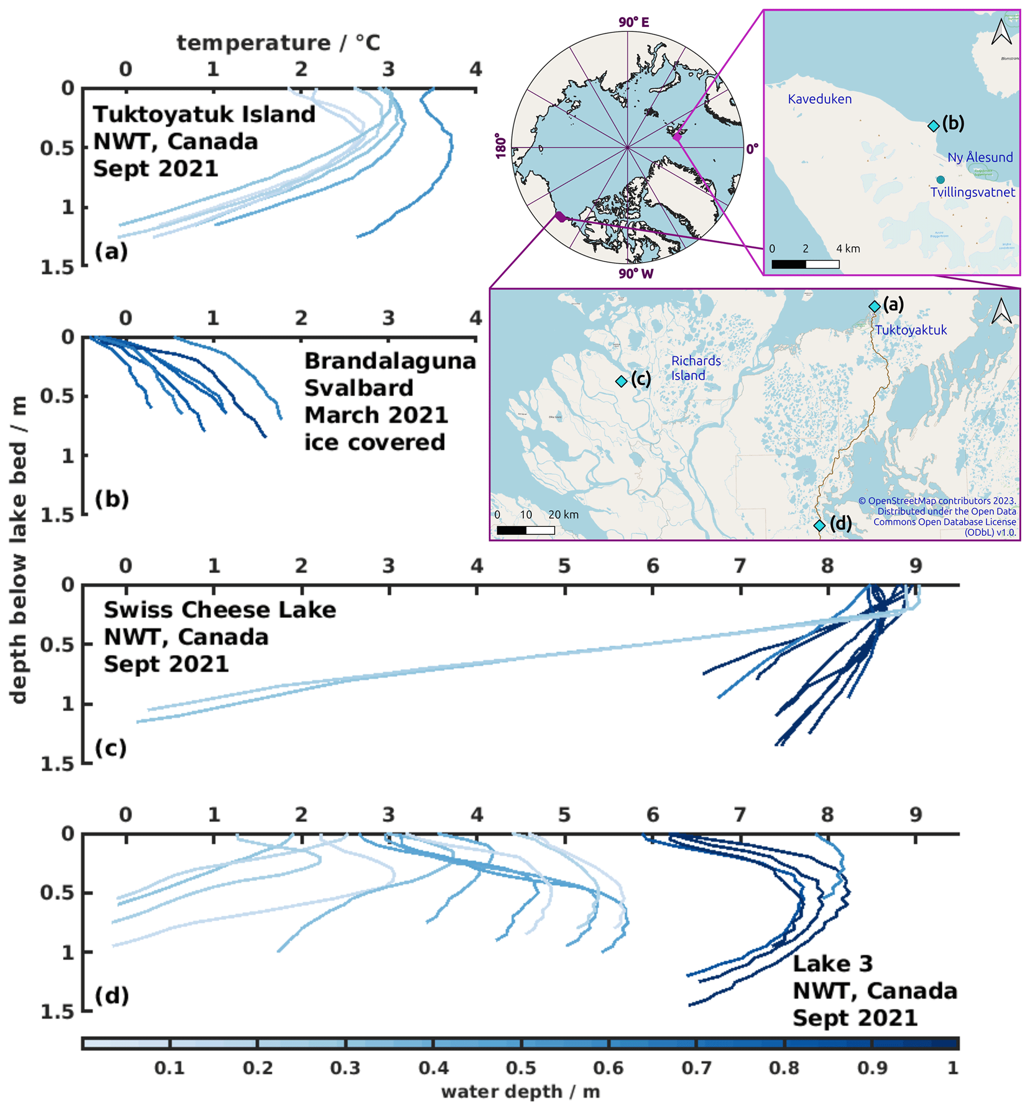
Figure 3Temperature–depth profiles grouped by investigation sites. The map shows all locations in teal diamonds and, additionally, the drinking-water lake of the long-term measurement as a circle. Map data are from https://www.openstreetmap.org/copyright (last access: 6 April 2024). (a) Measurements below the Arctic Ocean at Tuktoyaktuk Island, NWT, Canada. Measurements were taken from a wading position in the water in September 2021. (b) Measurements at Brandalaguna, Svalbard, were taken through an ≈60 cm ice cover in March 2021. (c) Measurements at Swiss Cheese Lake in the outer Mackenzie River Delta, NWT, Canada, were taken from a small rubber boat in September 2021. (d) Measurements at Lake 3, near the Inuvik–Tuktoyaktuk Highway, NWT, Canada, were taken from a small rubber boat in September 2021. Brandalaguna and Tuktoyaktuk Island have brackish water, while the other two are freshwater lakes. The shades of blue indicate water depth, and the scale is the same over all sites. We measured in water as deep as 2.5 m (at Swiss Cheese Lake), but the color scale is cropped to 1 m to better distinguish between shallower values.
We observe that measurements at all locations reveal spatial heterogeneity in sediment temperatures and a difference between the locations even at the same water depth. Water depth alone is not able to cluster the measured temperature–depth profiles over all sites.
The importance of the spatial heterogeneity in shallow water is possibly linked to zones with bed-fast ice. Permafrost may be found under lakes with bed-fast ice regimes (Arp et al., 2016), while floating-ice lakes may develop taliks (Boike et al., 2015; Arp et al., 2016; Burn, 2002). Burn (2002) monitored lake water and sediment temperatures during 1992–1996 at various lakes on Richards Island, Northwest Territories (see Fig. 3). They found permafrost below the terraces with water depth shallower than ≈60 % of the maximum ice thickness (i.e., shallower than 1 m). The measured mean annual lake-bottom-water temperatures in these shallow parts varied, however, over a wide range, from −6 to 0 °C. Our observations at Swiss Cheese Lake corroborate these findings.
Our newly built temperature lance has proven suitable for use in a variety of Arctic aquatic environments. It is portable enough to be brought along on helicopter flights and carried on foot over the tundra. It was successfully used in winter through lake ice and in summer from a rubber boat and by wading in shallow water. The maximum penetration depth when hand-operated varies with the structure of the sediment, with fine sands being ideal. Hammering the lance was only moderately successful in increasing penetration depth. Extracting the lance was easiest from the boat, using the steady up-and-down rhythm of the boat in the waves. This indicates that vibrating the lance in, with either a motor or a drop weight, could be another option for deployment with more reliable deeper penetration.
The equilibration time depended largely on the sediment's thermal properties and the initial temperature gradient between the lance and the sediment but was overall short enough to be able to acquire measurements in under 1 h, including the time needed to push the lance into the sediment and to recover it. We recommend leaving the device in the sediment for more than 30 min to ensure sufficient thermal equilibration with the sediment. Using an inversion algorithm to retrieve an estimate of the asymptotic in situ temperatures improves the accuracy of the resulting temperature–depth profile, especially for short measurements, but this advantage fades when the measurement is long enough to have good accuracy.
The presented data show significant variation between the spatially distributed temperature–depth profiles obtained at each site and captured spatial heterogeneity that would be unavailable from single boreholes. We observe similar temperature–depth profiles in the deeper water (>1 m) at each location and large variability (up to 5 °C) in shallower water (<0.9 m). Lake sediment temperatures in shallow waters tend to show higher spatial heterogeneity. Single-location sediment temperature profiles – for example, from boreholes – cannot capture the variety in the temperature field. Our measurements can capture this variety but would require repeat deployments to capture temporal variability.
The resulting data sets will bring new insights into the temperature dynamics under shallow lakes, especially in the bottom-fast ice zone. Data from locations like Swiss Cheese Lake can help to better constrain patterns of methane emissions and support investigations of the sources (Wesley et al., 2022). These data are suitable as validation for modeling, can give additional spatial information around borehole installations, and may yield insights into heat fluxes at the sediment–water interface. Future work will focus on estimating the permafrost table from these measurements via extrapolation and thermal modeling.
The data are available from Pangaea, and the references are provided in Table 1.
FM, WLC, PPO, and JB conceptualized the design of the lance and the fieldwork. WLC constructed the devices with the assistance of FM and wrote the logger code. FM, WLC, and JB carried out the fieldwork. FM analyzed the data and wrote the paper. JB and PPO acquired the funding. All authors contributed to the final paper.
The contact author has declared that none of the authors has any competing interests.
Publisher’s note: Copernicus Publications remains neutral with regard to jurisdictional claims made in the text, published maps, institutional affiliations, or any other geographical representation in this paper. While Copernicus Publications makes every effort to include appropriate place names, the final responsibility lies with the authors.
This work is part of the Helmholtz Association as part of the MOSES (Modular Observation Solutions for Earth Systems) project. The authors would like to thank the Scientific Workshop of the Alfred Wegener Institute in Bremerhaven for design assistance and manufacturing the lance body and extensions.
The article processing charges for this open-access publication were covered by the Alfred-Wegener-Institut Helmholtz-Zentrum für Polar- und Meeresforschung.
This paper was edited by Adrian Flores Orozco and reviewed by Emmanuel Léger and one anonymous referee.
Abnizova, A., Siemens, J., Langer, M., and Boike, J.: Small ponds with major impact: The relevance of ponds and lakes in permafrost landscapes to carbon dioxide emissions, Global Biogeochem. Cy., 26, GB2041, https://doi.org/10.1029/2011GB004237, 2012. a
Arp, C. D., Jones, B. M., Grosse, G., Bondurant, A. C., Romanovsky, V. E., Hinkel, K. M., and Parsekian, A. D.: Threshold sensitivity of shallow Arctic lakes and sublake permafrost to changing winter climate, Geophys. Res. Lett., 43, 6358–6365, https://doi.org/10.1002/2016GL068506, 2016. a, b, c
Boike, J., Georgi, C., Kirilin, G., Muster, S., Abramova, K., Fedorova, I., Chetverova, A., Grigoriev, M., Bornemann, N., and Langer, M.: Thermal processes of thermokarst lakes in the continuous permafrost zone of northern Siberia – observations and modeling (Lena River Delta, Siberia), Biogeosciences, 12, 5941–5965, https://doi.org/10.5194/bg-12-5941-2015, 2015. a, b
Brown, W. G., Johnston, G. H., and Brown, R. J. E.: Comparison of observed and calculated ground temperatures with permafrost distribution under a northern lake, Can. Geotech. J., 1, 147–154, https://publications-cnrc.canada.ca/eng/view/object/?id=0b9d85f6-dfa9-499c-b29d-6dfe5bcd34c8 (last access: 8 May 2024), 1964. a
Bullard, E.: The Flow of Heat through the Floor of the Atlantic Ocean, in: Proceedings of the Royal Society A: Mathematical, Physical and Engineering Sciences, 222, 408–429, https://doi.org/10.1098/rspa.1954.0085, 1954. a, b
Burn, C. R.: Tundra lakes and permafrost, Richards Island, western Arctic coast, Canada, Can. J. Earth Sci, 39, 1281–1298, https://doi.org/10.1139/E02-035, 2002. a, b, c, d
Carslaw, H. S. and Jaeger, J. C.: Conduction of Heat in Solids, Oxford University Press, Oxford, ISBN: 0198533039, 1959. a
Christoffel, D. A. and Calheam, I. M.: A geothermal heat flow probe for in situ measurement of both temperature gradient and thermal conductivity, J. Phys. E Sci. Instrum., 2, 457–465, 1969. a, b
Dafflon, B., Wielandt, S., Lamb, J., McClure, P., Shirley, I., Uhlemann, S., Wang, C., Fiolleau, S., Brunetti, C., Akins, F. H., Fitzpatrick, J., Pullman, S., Busey, R., Ulrich, C., Peterson, J., and Hubbard, S. S.: A distributed temperature profiling system for vertically and laterally dense acquisition of soil and snow temperature, The Cryosphere, 16, 719–736, https://doi.org/10.5194/tc-16-719-2022, 2022. a
Dziadek, R., Doll, M., Warnke, F., and Schlindwein, V.: Towards closing the polar gap: New marine heat flow observations in antarctica and the Arctic ocean, Geosciences, 11, 11, https://doi.org/10.3390/geosciences11010011, 2021. a
Hartmann, A. and Villinger, H.: Inversion of marine heat flow measurements by expansion of the temperature decay function, Geophys. J. Int., 148, 628–636, https://doi.org/10.1046/j.1365-246X.2002.01600.x, 2002. a
Hornbach, M. J., Sylvester, J., Hayward, C., Kühn, M., Huhn-Frehers, K., Freudenthal, T., Watt, S. F., Berndt, C., Kutterolf, S., Kuhlmann, J., Sievers, C., Rapp, S., Pallapies, K., Gatter, R., and Hoenekopp, L.: A Hybrid Lister-Outrigger Probe for Rapid Marine Geothermal Gradient Measurement, Earth and Space Science, 8, e2020EA001327, https://doi.org/10.1029/2020EA001327, 2021. a
Hyndman, R. D., Davis, E. E., and Wright, J. A.: The Measurement of Marine Geothermal Heat Flow by a Multipenetration Probe with Digital Acoustic Telemetry and Insitu Thermal Conductivity, Mar. Geophys. Res., 2, 181–205, 1979. a, b
Jorgenson, M. T., Romanovsky, V., Harden, J., Shur, Y., O’Donnell, J., Schuur, E. A. G., Kanevskiy, M., and Marchenko, S.: Resilience and vulnerability of permafrost to climate change, Can. J. Forest Res., 40, 1219–1236, https://doi.org/10.1139/X10-060, 2010. a
Lindqvist, J. G.: Heat Flow Density Measurements in the Sediments of three Lakes in Northern Sweden, Tectonophysics, 103, 121, 1984. a, b
Lister, C. R.: Measurement of in Situ Sediment Conductivity by means of a Bullard‐type Probe, Geophys. J. Roy. Astr. S., 19, 521–532, https://doi.org/10.1111/j.1365-246X.1970.tb00157.x, 1970. a, b, c
Miesner, F., Boike, J., and Cable, W. L.: Physical oceanography (CTD) measurements in Brandallaguna in March 2021, PANGAEA [data set], https://doi.org/10.1594/PANGAEA.951082, 2022a. a, b
Miesner, F., Cable, W. L., and Boike, J.: Temperature measurements at Brandallaguna in March 2021, PANGAEA [data set], https://doi.org/10.1594/PANGAEA.950782, 2022b. a, b
Miesner, F., Cable, W. L., and Boike, J.: Temperature measurements at three subaquatic sites in the Mackenzie Delta, Northwest Territories, Canada, PANGAEA [data set], https://doi.org/10.1594/PANGAEA.949290, 2022c. a, b, c
Miesner, F., Erkens, E., Boike, J., and Overduin, P. P.: CTD measurements acquired in a small lake (“Lake 3”) between the villages of Tuktoyaktuk and Inuvik, Canada, PANGAEA [data set], https://doi.org/10.1594/PANGAEA.949253, 2022d. a
Miesner, F., Erkens, E., Boike, J., and Overduin, P. P.: CTD measurements acquired in a former river channel (“Swiss Cheese Lake”) in the Mackenzie Delta, Northwest Territories, Canada, PANGAEA [data set], https://doi.org/10.1594/PANGAEA.949256, 2022e. a
Miesner, F., Erkens, E., Boike, J., and Overduin, P. P.: CTD measurements acquired in the region of Tuktoyaktuk Island, Northwest Territories, Canada, PANGAEA [data set], https://doi.org/10.1594/PANGAEA.949258, 2022f. a
Onken, R., Garbe, H., Schröder, S., and Janik, M.: A new instrument for sediment temperature measurements, J. Mar. Sci. Technol., 15, 427–433, https://doi.org/10.1007/s00773-010-0096-8, 2010. a
Paltan, H., Dash, J., and Edwards, M.: A refined mapping of Arctic lakes using Landsat imagery, Int. J. Remote Sens., 36, 5970–5982, https://doi.org/10.1080/01431161.2015.1110263, 2015. a
Riedel, M., Villinger, H., Asshoff, K., Kaul, N., and Dallimore, S. R.: Temperature measurements and thermal gradient estimates on the slope and shelf-edge region of the Beaufort Sea, Canada, Geological Survey of Canada, Open File, 7725, https://doi.org/10.4095/296570, 2015. a
Roy-Leveillee, P. and Burn, C. R.: Near-shore talik development beneath shallow water in expanding thermokarst lakes, Old Crow Flats, Yukon, J. Geophys. Res.-Earth, 122, 1070–1089, https://doi.org/10.1002/2016JF004022, 2017. a
Sclater, J. G., Corry, C. E., and Vacquier, V.: In Situ Measurement of the Thermal Conductivity of Ocean-Floor Sediments, J. Geophys. Res., 74, 1070–1081, https://doi.org/10.1029/jb074i004p01070, 1969. a
Solomon, S. M., Taylor, A. E., and Stevens, C. W.: Nearshore Ground Temperatures, Seasonal Ice Bonding, and Permafrost Formation Within the Bottom-Fast Ice Zone, Mackenzie Delta, NWT, in: Proceedings of the Ninth International Conference on Permafrost, Fairbanks, Alaska, June 29–July 3, edited by: Kane, D. L. and Hinkel, K. M., vol. 2, 1675–1680, http://uspermafrostold.org/icop-proceedings/9th International Conference on Permafrost Vol 2.pdf (last access: 8 May 2024), 2008. a
Wesley, D., Dallimore, S., MacLeod, R., Sachs, T., and Risk, D.: Characterization of atmospheric methane release in the outer Mackenzie River delta from biogenic and thermogenic sources, The Cryosphere, 17, 5283–5297, https://doi.org/10.5194/tc-17-5283-2023, 2023. a
Whalen, D., Forbes, D., Kostylev, V., Lim, M., Fraser, P., Nedimović, M., and Stuckey, S.: Mechanisms, volumetric assessment, and prognosis for rapid coastal erosion of Tuktoyaktuk Island, an important natural barrier for the harbour and community, Can. J. Earth Sci., 59, 945–960, https://doi.org/10.1139/cjes-2021-0101, 2022. a
Wise, J. A.: Liquid-in-glass thermometer calibration service, NIST measurement sercives, Vol. 250, No. 23, US Department of Commerce, National Institute of Standards and Technology, https://nvlpubs.nist.gov/nistpubs/Legacy/SP/nistspecialpublication250-23.pdf (last access: 8 May 2024), 1988. a