A large-scale high-resolution numerical model for sea-ice fragmentation dynamics

Forecasts of sea-ice motion and fragmentation are of vital importance for all human interactions with sea ice, ranging from those involving indigenous hunters to shipping in polar regions. Sea-ice models are also important for simulating long-term changes in a warming climate. Here, we apply the Helsinki Discrete Element Model (HiDEM), originally developed for glacier calving, to sea-ice breakup and dynamics. The code is highly optimized to utilize high-end supercomputers to achieve an extreme time and space resolution. Simulated fracture patterns and ice motion are compared with satellite images of the Kvarken region of the Baltic Sea from March 2018. A second application of HiDEM involves ice ridge formation in the Gulf of Riga. With a few tens of graphics processing units (GPUs), the code is capable of reproducing observed ice patterns that in nature may take a few days to form; this is done over an area of $\sim \mathrm{100}\mathrm{km}\times \mathrm{100}\mathrm{km}$, with an 8 m resolution, in computations lasting ∼10 h. The simulations largely reproduce observed fracture patterns, ice motion, fast-ice regions, floe size distributions, and ridge patterns. The similarities and differences between observed and computed ice dynamics and their relation to initial conditions, boundary conditions, and applied driving forces are discussed in detail. The results reported here indicate that the HiDEM has the potential to be developed into a detailed high-resolution model for sea-ice dynamics at short timescales, which, when combined with large-scale and long-term continuum models, may form an efficient framework for forecasts of sea-ice dynamics.

1 Introduction

Reliable forecast models for ice dynamics are of vital importance for all human activities related to sea ice. Indigenous hunters in the Arctic can move fast over long distances across level landfast ice, while traveling on drift ice or on land can be immensely more difficult. Similarly, sustainable and safe winter navigation is dependent on ice conditions, requiring constant route optimizations to avoid packed or ridged ice. Sea ice also influences the design of offshore structures, such as wind turbines, and in cold regions, sea ice may be a hindering factor for renewable energy. In addition, a large-scale implementation of offshore wind farms may affect local sea-ice dynamics. For all these purposes, new high-resolution ice models that are capable of simulating ice dynamics across tens to hundreds of kilometers are needed.

Traditionally, large-scale continuum models have been used for modeling sea-ice dynamics at scales larger than kilometer scales. Such models are computationally efficient and can easily be extended over larger areas and longer durations compared to the discrete-element-method (DEM) approach used here. A well-known challenge of continuum models is that an effective rheology for sea ice has to be implemented in the model, and there is no easy and straight-forward way to model all relevant aspects of sea-ice dynamics using an effective large-scale rheology. Some of the early attempts in this direction include the viscoplastic model (Hibler, 1977, 1979), developed in the 1970s. The viscoplastic model by Hibler can capture some effective large-scale ice dynamics but fails to model the formation of leads, compression ridges, shear zones, and floe fields that are apparent at scales smaller than ∼ 100 km. More advanced and more accurate continuum models include the elastic-decohesive model by Schreyer et al. (2006), the Maxwell elasto-brittle model by Dansereau et al. (2016), and the brittle Bingham–Maxwell rheology model by Ólasson et al. (2022). Several modern high-resolution continuum models are able to capture many of the characteristics of large-scale fracturing (Bouchat et al., 2022; Hutter et al., 2022), and some are even utilized as operational application tools with a grid resolution of a few kilometers (Pemberton et al., 2017; Kärnä et al., 2021; Röhrs et al., 2023). However, even advanced and modern continuum models struggle with modeling fine-scale details, such as leads and ridges.

DEM models take a significantly different approach. Instead of modeling sea ice as a continuum, solid and elastic blocks are initially connected together to form sea ice. The dynamics are typically computed via discrete versions of Newton's equations with some form of energy dissipation term. When a load is applied, these connections may break, and ice disintegrates into discrete floes. Early models of this kind utilized circular discrete elements (DEs) moving in two dimensions (Babic et al., 1990; Hopkins and Hibler, 1991; Blockley et al., 2020). Hopkins and Thorndike (2006) modeled Arctic pack ice using a DE model. The resolution of these models was not enough to resolve details; instead, important features, such as ridging, were described by an ice floe interaction model. A similar approach was later adopted by West et al. (2022), who simulated ice dynamics in the Nares Strait, and by Damsgaard et al. (2021, 2018), who investigated pressure ridging. Also, a recent investigation by Manucharyan and Montemuro (2022), which introduced complex discrete elements with time-evolving shapes, relied on a similar approach. In addition, they used a rudimentary fracture model to describe the failure of sea ice. Our model is not based on these models; instead, we explicitly model ice dynamics at a scale on the order of meters, including ridging, leads, and shear and tensile fractures, with large-scale ice failure patterns emerging as a collective result of these smaller-scale failure processes. Our model also does not rely on an assumption of ice floes; instead, we let the ice floes form and fracture throughout the simulations.

The objective of this investigation is to bridge the gaps between continuum models and DE models by implementing and testing a computationally efficient DEM that has been developed and optimized for high-end computing using vast numbers of highly efficient processors. If a detailed high-fidelity model of this kind can be scaled up to length scales at which continuum models are sufficient, and if the two types of models can be combined to form a unified framework, a very useful forecast model for sea-ice dynamics would be the result.

2 The Helsinki Discrete Element Model (HiDEM) for sea ice

2.1 Mechanics of the HiDEM

The HiDEM code uses a discrete-element-method (DEM) algorithm. A DEM formulation for sea-ice motion may be related to the Cauchy momentum equation (Acheson, 1990), which treats sea ice as a continuum. In its full form, this equation accounts for the Coriolis force, atmospheric and ocean stresses, sea surface tilt, and Cauchy stresses within pack ice. The Cauchy momentum equation reads

$$\begin{array}{}\text{(1)}& m\left({\displaystyle \frac{\mathrm{D}\mathit{u}}{\mathrm{D}t}}+f\mathit{k}\times \mathit{u}\right)={\mathit{\tau }}^{\mathrm{a}}+{\mathit{\tau }}^{\mathrm{w}}+m\mathit{g}\mathrm{\Delta }H+\mathbf{\nabla }\cdot \mathit{\sigma },\end{array}$$

where m is the combined ice and snow mass, u is the horizontal ice velocity vector, f is the Coriolis parameter, k is the upward unit vector, τ^a and τ^w are the stresses due to air and water drag, g is the gravitational acceleration, ΔH is the vertical component of the sea surface tilt, and σ is the Cauchy stress tensor of ice.

Below, we focus on short-term sea-ice deformations driven by external forcing and modified by coastal boundary conditions and sea-ice fracturing. In this case, we can neglect the Coriolis term and the sea surface tilt, which results in the previous equation becoming

$$\begin{array}{}\text{(2)}& m{\displaystyle \frac{\mathrm{D}\mathit{u}}{\mathrm{D}t}}={\mathit{\tau }}^{\mathrm{a}}+{\mathit{\tau }}^{\mathrm{w}}+\mathrm{\nabla }\cdot \mathit{\sigma }.\end{array}$$

Assuming a simple linear Kelvin–Voigt type of viscoelasticity (Meyers and Chawla, 2009), the stress tensor of sea ice can be written as

$$\begin{array}{}\text{(3)}& \mathit{\sigma }=A\dot{\mathit{ϵ}}+B(\mathit{x},t)\mathit{ϵ},\end{array}$$

where A represents dissipative deformations, such as viscosity, and B(x,t) represents spatially and temporally varying brittle elasticity. Here, σ denotes stress, ϵ denotes strain, and $\dot{\mathit{ϵ}}$ denotes strain rate.

DEM algorithms do not explicitly solve continuum equations but instead resolve forces on interacting DEs. The continuum equations above can be reformulated in a format more suitable for a DEM implementation. DEs interact pairwise either through beams connecting them or through repulsive contact forces. If we define the discrete position vector x_i of the DE i, which includes 3 translational and 3 rotational degrees of freedom, the DEM equation of motion can be written as

$$\begin{array}{}\text{(4)}& m_i{\ddot{\mathit{x}}}_i+\sum _j\mathbf{K}{\mathit{x}}_{ij}+\sum _j{C}_{\mathrm{2}}{\dot{\mathit{x}}}_{ij}+C_{\mathrm{1}}{\dot{\mathit{x}}}_i={\mathit{F}}_i,\end{array}$$

where m_i is the mass or moment of inertia of i, C₁ is the drag coefficient of the combined drag of water and air, and F_i denotes external forces and moments (such as gravity and buoyancy). Further, K=K(t) and C₂=C(t) represent elements of contact stiffness and damping matrices for the interacting discrete-element pair i and j, and x_ij refers to the position vector between i and its neighbor j. Moreover, $\dot{\mathit{x}}$ and $\ddot{x}$ are the first and second time derivatives of x. K and C₂ correspond to B and A in Eq. (3), respectively, and depending on the pair of discrete elements, they may include elements of stiffness and damping matrices concerning either the beams or the repulsive contacts of the discrete elements.

In the previous equation, ${\sum }_j\mathbf{K}{\mathit{x}}_{ij}+{\sum }_j{C}_{\mathrm{2}}{\dot{\mathit{x}}}_{ij}$ corresponds to ∇⋅σ in Eq. (2), with the divergence operator being replaced by a sum of all neighboring discrete elements of i. This can be done as the contact forces from neighbors on opposite sides of a discrete element cancel each other out if they apply equal force on i; thus, only change in the force across an element induces motion. Further, $C_{\mathrm{1}}{\dot{\mathit{x}}}_i$ and F_i in Eq. (4) include the effect of stresses τ^a and τ^w in Eq. (2). DEM simulations utilize explicit time stepping. For this, the previous equation can be written in discrete form using the definition of the derivatives, and the motion of the discrete elements, x(t+dt) as a function of x(t) and x(t−dt), can be computed via iterations of time steps (dt) based on element positions, velocities, and forces acting on them.

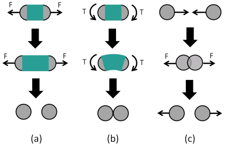
Figure 1 In a DEM algorithm, an intact material is described by joining discrete elements (here shown as circular in shape) with beams. (a) Tensile forces (F) break a beam connecting DEs if stretched beyond a certain limit. (b) Torque (T) also breaks a beam if the difference in rotation angles is too large. (c) DEs also interact through pairwise inelastic collisions (Riikilä et al., 2015).

2.2 Code optimization for high-performance computing

Any computational implementation of Eq. (4) involves a trade-off between accuracy and computational efficiency. A higher accuracy could mean, for example, including irregular elements, higher-order time integration schemes, nonlinear elasticity, and/or nonlinear drag coefficients. In contrast, simpler models with a higher computational efficiency allow for a finer resolution, i.e., smaller elements and time steps. The HiDEM is focused on the latter. In the DEM algorithm, a large set of elements move relative to each other and interact only with neighbors within a limited maximum interaction range. Most of the computational effort for algorithms of this kind has to be dedicated to computing forces between elements. With such a code structure, the HiDEM is a good candidate for efficient implementation on the most powerful and modern high-performance computers (HPCs). The HiDEM code is written in C++ using the Message Passing Interface (MPI) and Open Multi-Processing (OpenMP) version 4.x or higher for parallelization and multithreading. Offloading to graphics processing units (GPUs) is done using CUDA or HIP. The code is optimized for maximum computational efficiency on supercomputers or large clusters with an efficient interconnect. The code can be compiled to run only on CPUs or on a combination of CPUs and GPUs (with almost all computations occurring on GPUs).

The HiDEM code thus has two levels of parallelization by means of two different methods: MPI message passing between the CPU nodes and OpenMP multithreading on CPUs with many compute cores or, alternatively, employing the MPI for CPUs and using CUDA or HIP to offload the most compute-intensive parts to GPUs. This structure introduces a high level of complexity to the code, and extreme care has been taken to implement optimal data structures and communications so that the compute power of the GPUs can be utilized as efficiently as possible. The technical details of the code's data structures and communication schemes are beyond the scope of this article and will be reported elsewhere.

The results reported here were run on the Large Unified Modern Infrastructure (LUMI) supercomputer in Kajaani, Finland. In June 2023, LUMI was ranked third on the TOP500 list of the world's fastest supercomputers. The LUMI GPU partition has 2928 GPU nodes, each equipped with a 64-core CPU and eight Graphics Compute Dies (GCDs). For the results reported here, we performed runs using about 100 million elements with roughly half a billion interactions and a few million time steps. A simulation typically lasted about 10–20 h, and we used no more than four GPU nodes. Hence, there is still a lot of potential to scale up the element count and increase the time integration speed. The extreme computational efficiency of the HiDEM code when implemented in a suitable HPC environment allows for extreme scale and resolution properties, thus setting the HiDEM apart from standard DEMs. DEM results cited in the Introduction typically report models with approximately 10 000 elements or, for some larger numbers of elements, significantly larger time steps for kilometer-sized elements. The resolution of the HiDEM simulations is demonstrated in Fig. 2b, which displays only 1 % of the Kvarken simulation domain in order to make details visible. This figure also displays how damaged ice (i.e., drift ice) and undamaged ice (i.e., landfast ice) can behave differently in the model.

2.3 Sea-ice simulations

The purpose of this investigation is to apply a simple and computationally efficient DEM implementation, as described above, to simulate sea-ice fragmentation and compare the result with observations. We apply the HiDEM code to ice failure in the Kvarken region of the Baltic Sea and to ridge formation in the Gulf of Riga (Fig. 2). Our objective is to investigate the model's capability to mimic the ice dynamics in Kvarken – this is a narrow strait that is often ice-covered on its northeastern (NE) side, while the sea often remains largely open on its southwestern (SW) side, creating interesting dynamics when wind pushes ice towards the southwest. Our second objective is to test how well the model mimics the formation of ice compression ridges in the Gulf of Riga under strong SW winds. This is a well-known problem for shipping in this region.

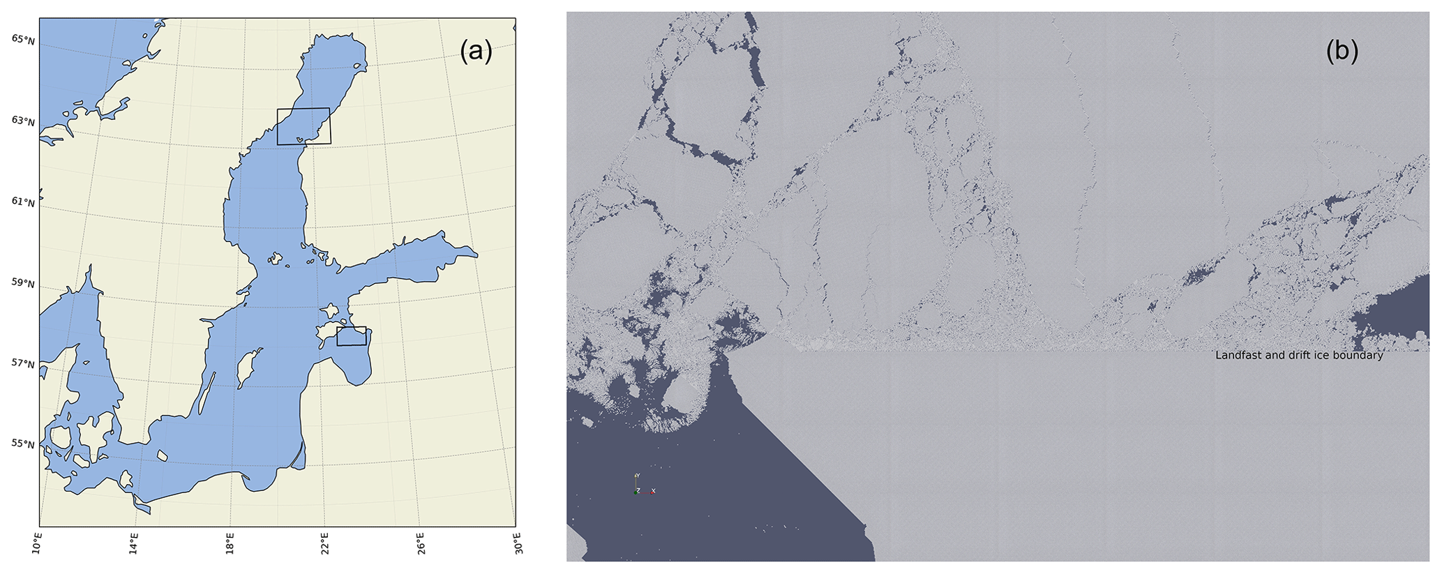
Figure 2 (a) The two simulation domains in Kvarken and the Gulf of Riga, indicated by rectangles. (b) All DEs displayed in a $\sim \mathrm{10}\mathrm{km}\times \mathrm{7}\mathrm{km}$ area in the southwestern corner of the Kvarken simulation domain at a late stage of the 8 March 2018 simulation when the ice is broken up. The straight boundary from east to west, between the drift ice and landfast ice, is indicated in the figure.

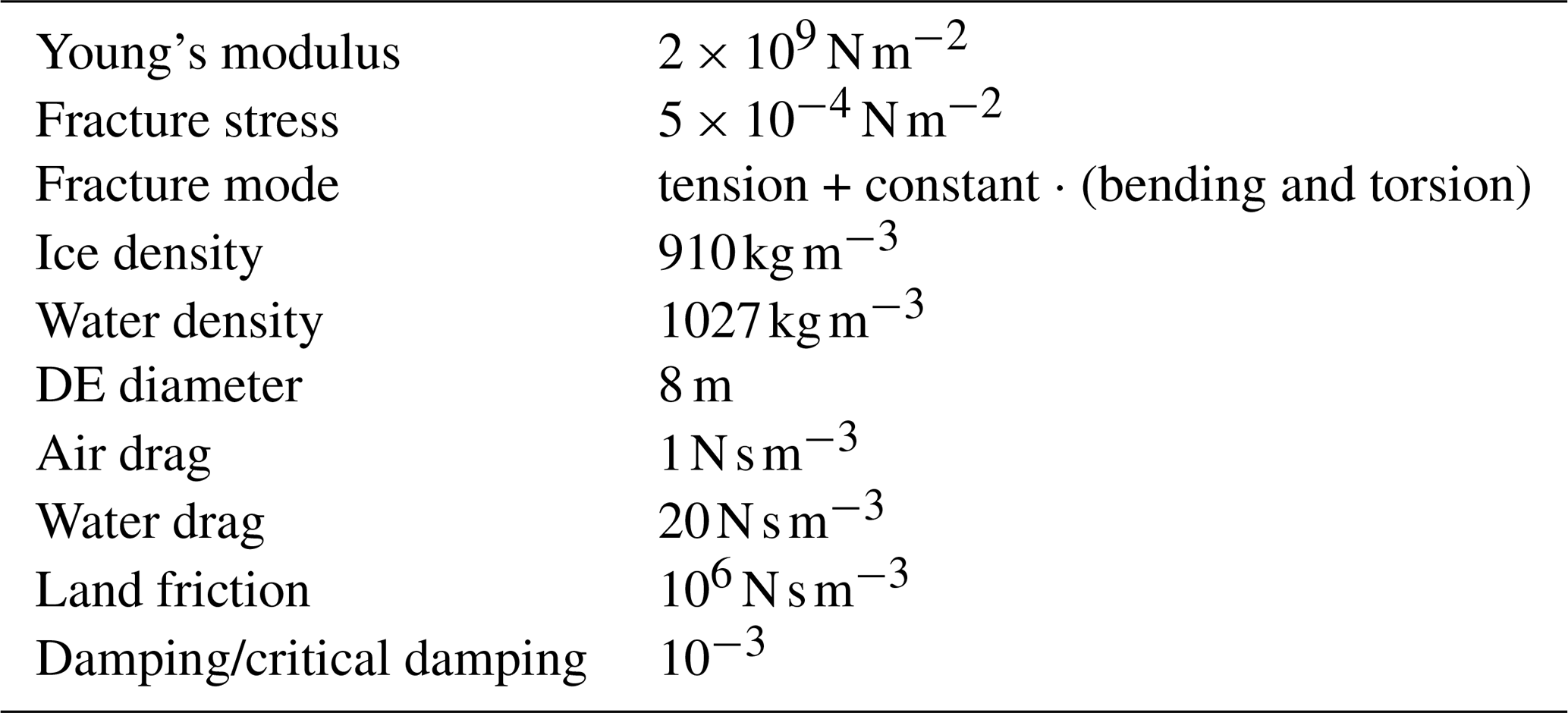
We use closely packed spherical DEs, all of a similar size and 8 m in diameter, connected by Euler–Bernoulli beams. A beam connects two center points of a DE. Each DE, and therefore also each endpoint of a beam, has 6 degrees of freedom: 3 translational and 3 rotational degrees of freedom. Beams connect either all or a fraction of the randomly selected nearest neighbors. The matrix K in Eq. (4) contains the stiffness elements (or spring constants) that relate forces and torques to beam deformation. The stiffness matrix of a single beam, along with other details, is given in Åström et al. (2013). All relations between forces and deformations are linear up to a beam's breaking point, which is determined by the beam deformations (either as an elastic energy criterion or as a maximum stress/strain criterion). Once a beam breaks, it vanishes – i.e., the connection between the DEs is irreversibly broken, and the DEs can freely move apart but will continue to interact if they are pressed against each other. DEM parameters are listed in Table 1. Drag and friction terms are linear in velocity. Drag coefficients are small to allow for swift dynamics. Land friction is high to prevent ice from sliding onto land. Damping is small compared to the critical damping of a harmonic oscillator to allow sound waves to travel through the ice; however, it is large enough to prevent the buildup of vibrational kinetic energy in the ice. The element interactions are sketched in Fig. 1. The animation in the “Video supplement” demonstrates simulated ice dynamics in a small fraction (∼0.3 %) of the Kvarken domain so that details can be seen.

Table 1 HiDEM parameters.

The typical winter sea-ice thickness in the Kvarken region is on the order of 1 m or less. This means an accurate ice thickness can only be described explicitly if the diameter of the spherical elements is no more than 1 m. This would increase computational requirements immensely compared to when 8 m spheres are used in the large-scale simulations. The number of elements would have to be increased by a factor of 64 to simulate the same domain. Instead, we use a single layer of DEs in a closely packed configuration that forms a triangular lattice of 8 m spheres.

A consequence of the 8 m diameter is that the model ice will be significantly thicker and stronger than the ice that appears naturally in the region. Ice fractures when stress buildup reaches the fracture threshold of the ice. When the ice breaks, stress is relieved. In order to simulate this, we can define a dimensionless parameter, R_ss, which represents the ratio of the stress of the model ice to its strength, and tune the applied stress on the ice in the simulations so that this ratio is approximately equal to unity. The stress-to-strength ratio of the model ice is given by

$$\begin{array}{}\text{(5)}& R_{\mathrm{ss}}={\displaystyle \frac{h{l}_{\mathrm{DE}}{E}_{\mathrm{ice}}{\mathit{ϵ}}_{\mathrm{frac}}}{f_{\mathrm{DE}}{L}_{\mathrm{domain}}/l_{\mathrm{DE}}}},\end{array}$$

where h is ice thickness, l_DE is the horizontal dimension of the DEs, E_iceϵ_frac is the ice fracture stress, f_DE is the force applied on each DE, and $L_{\mathrm{domain}}/l_{\mathrm{DE}}$ is the relative resolution of the simulation domain. R_ss is of order 1, as it should be if we use the following: h=1, l_DE=8, a driving force on the order of 100 N/DE, an ice fracture stress of order 10⁵ N m⁻², and $L_{\mathrm{domain}}/l_{\mathrm{DE}}\sim {\mathrm{10}}^{\mathrm{4}}$. Benefits of increasing f_DE, while keeping R_ss fixed, is that ice dynamics can be made a bit faster and that forecasts corresponding to longer times can be performed using shorter simulations.

The triangular lattice structure introduces a weak anisotropy in the material stiffness and limits the crack propagation directions to a few preferred ones on the scale of a DE. The triangular lattice has three possible crack propagation directions, with a 60° angle between them. These angles are, however, not visible in the larger-scale fracture patterns in, for example, Fig. 2b. This means that, on a large scale, the model behaves predominantly isotropically, as it should.

In spite of the limitations, the lack of detail in the initial and boundary conditions, the driving forces, and the simplicity of the DEM implementation, the model is – as demonstrated below – able to capture a great deal of the large-scale structures and small-scale details of observed sea-ice fragmentation and dynamics.

3 Kvarken region – March 2018

Kvarken is the narrow and shallow neck between the Bay of Bothnia and the rest of the Gulf of Bothnia. In a typical winter, such as the winter of 2018, the Bay of Bothnia freezes over completely, while the rest of the Gulf of Bothnia freezes only partly. This makes Kvarken an interesting location for ice dynamics because, when subjected to strong northern or eastern winds, the sea ice in the Bay of Bothnia is fragmented and pushed through the narrow Kvarken Strait. During severe winters, ice arches can develop on the northern side of Kvarken. Physically, ice dynamics in Kvarken resemble those of the Nares Strait, where ice arching is common (Moore et al., 2023).

We simulate two different cases of ice dynamics, which occurred on 8 and 23 March 2018. For the simulation domain, we use a digital depth model (∼100 m resolution) of the Baltic Sea (courtesy of the Baltic Sea Hydrographic Commission), and for comparison with simulation results, we use Copernicus satellite images from the Landsat program (see the “Code and data availability” section). For forces driving the ice fragmentation, we mimic wind directions and magnitudes from weather data archives.

Initially, ice is set to cover the entire domain, except for a region southwest of the narrowest part of Kvarken, where we initially have a rectangular area of open water in order to roughly mimic the ice situation in March 2018. The northern and eastern domain boundaries are fixed, while the southern and western boundaries allow ice to flow out of the domain – except, of course, where land is blocking ice motion. The discrete-element diameter is 8 m, and we set the beam width to 40 % of the diameter. Further, we introduce disorder and strength variations in the ice by initially reducing the density of the beams from its maximum at uniformly random and uncorrelated locations. We use slightly different setups for the two cases: in the 23 March 2018 case, the density of the beams is reduced by 40 % over the entire domain, and in the 8 March 2018 case, for partly refrozen ice rubble that often appears at open sea, we reduce the density of the beams by 40 %, while fast-ice regions in the inner archipelago experience zero reduction in beam density. In terms of ice strength, this corresponds to ice that is about 1.3 m thick.

3.1 Simulation case study for 23 March 2018

In the 23 March 2018 case, nearby weather stations reported moderate western winds early on 22 March 2018, which then strengthened and turned to northern winds at speeds of 9–11 m s⁻¹, before shifting to northeastern winds and eventually weakening during 23 March 2018. To model this, we applied a constant force from the north on all elements for 3 h, followed by 45 min of force from the northeast. In this case, as explained above, the ice is similar over the entire domain. Figure 3a displays the resulting ice motion, while Fig. 3b shows the largest compressive strains at the end of the simulation. These two figures show clearly the “bottleneck behavior” of ice motion through the Kvarken Strait. Ice that has passed southwest of the narrowest region moves fast, while compressive stresses are built up northeast of the narrowest region, leading to a reduction in ice speed. Ice is breaking up along compressive shear fracture zones, and some evidence of compressive arches is visible upwind of the narrowest point of the strait. Additional ice compression that is not related to ice motion through the strait is visible on the northern side of the Finnish archipelago.

Figure 3c depicts a satellite image of the Kvarken area on 23 March 2018. Correspondingly, Fig. 3d shows the simulated fracture pattern. The model-derived figure is rendered to mimic the satellite image, except for the fact that land is shown in brown so that it can be easily distinguished from open water. The similarity between these two images is striking, but there are also some noticeable inconsistencies. (i) There is significantly more open water east and north of Holmön (marked by “H” in Fig. 3a). This is most likely due to differences in initial conditions. In the simulations, the initial condition was that the Bay of Bothnia was 100 % ice-covered, while in reality, there was a wide expanse of open water along the Swedish coast in the days before 23 March 2018. (ii) Ice floes traveled much further through the Kvarken Strait in the satellite image compared to in the simulations, where the floes are closer to their original positions. The reason for this is simply that the simulation covers 3 h and 45 min of ice motion, while in reality, the motion lasted for about a day.

Figure 4a and b highlight the drift ice and landfast ice in both the satellite and simulated images. Likewise, in this case, the similarities between the two images are striking, but there are also visible differences – for example, the fairly straight southwest–northeast lead that marks the boundary between the drift ice and landfast ice goes a bit further to the north in the simulation compared to the satellite image. This lead begins near Valsörarna (marked by “V” in Fig. 4b) and reaches the Finnish coast at the island of Öuran (marked by “Ö”) in the satellite image and further north near the island of Torsön (marked by “T”) in the simulations.

Figure 4c and d highlight regions with highly disintegrated ice adjacent to the boundary between the drift ice and landfast ice. The reason why the ice becomes so crushed in this region is that it is pushed southwards by the wind, and high compressive forces will therefore appear on the northern side of the Finnish archipelago. The difference in the shape and extent of the simulated and observed crushed-ice regions is again a consequence of the shorter ice dynamics time in the simulations. A longer simulation would induce more shear crushing against the fast-ice margin as the drift ice slowly moves west through the Kvarken Strait. Another consequence of these particular dynamics is the appearance of east–west tensile stress in the drift ice region. Such stresses are typical of shear zones and often induce tensile cracks that are more or less perpendicular to the shear zone. Such cracks are marked by “C” in Fig. 4c and d.

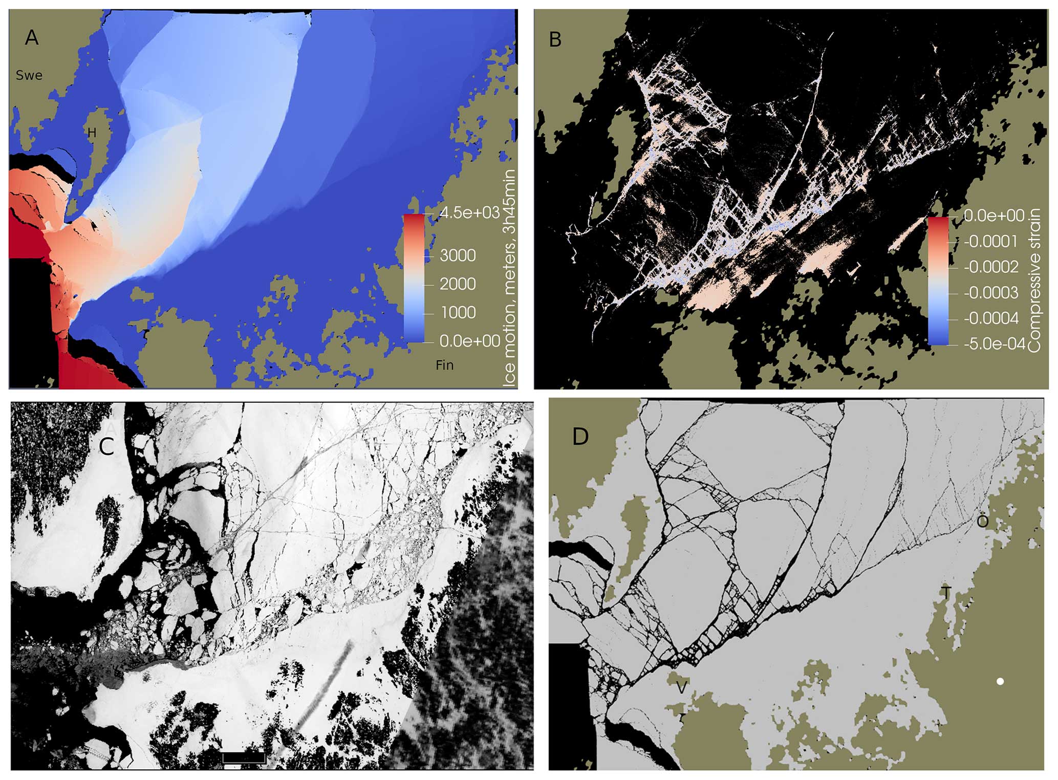
Figure 3 (a) Color-coded ice motion for the 23 March 2018 simulation. “Swe” and “Fin” mark the Swedish and Finnish mainlands. “H” marks the location of Holmön. (b) The largest compressive strains on intact beams connecting DEs at the end of the simulation. (c) A satellite image of the Kvarken area on 23 March 2018. “T” marks the location of the island of Torsön, “Ö” marks the location of the island of Öuran, and “V” marks the location of the island of Valsörarna. (d) The simulated fracture pattern after 3 h and 45 min. This image displays (with black dots) all beams that are strained to more than 5 % of their original length (and are thereby obviously broken). Water is depicted in black, ice in gray, and land in brown.

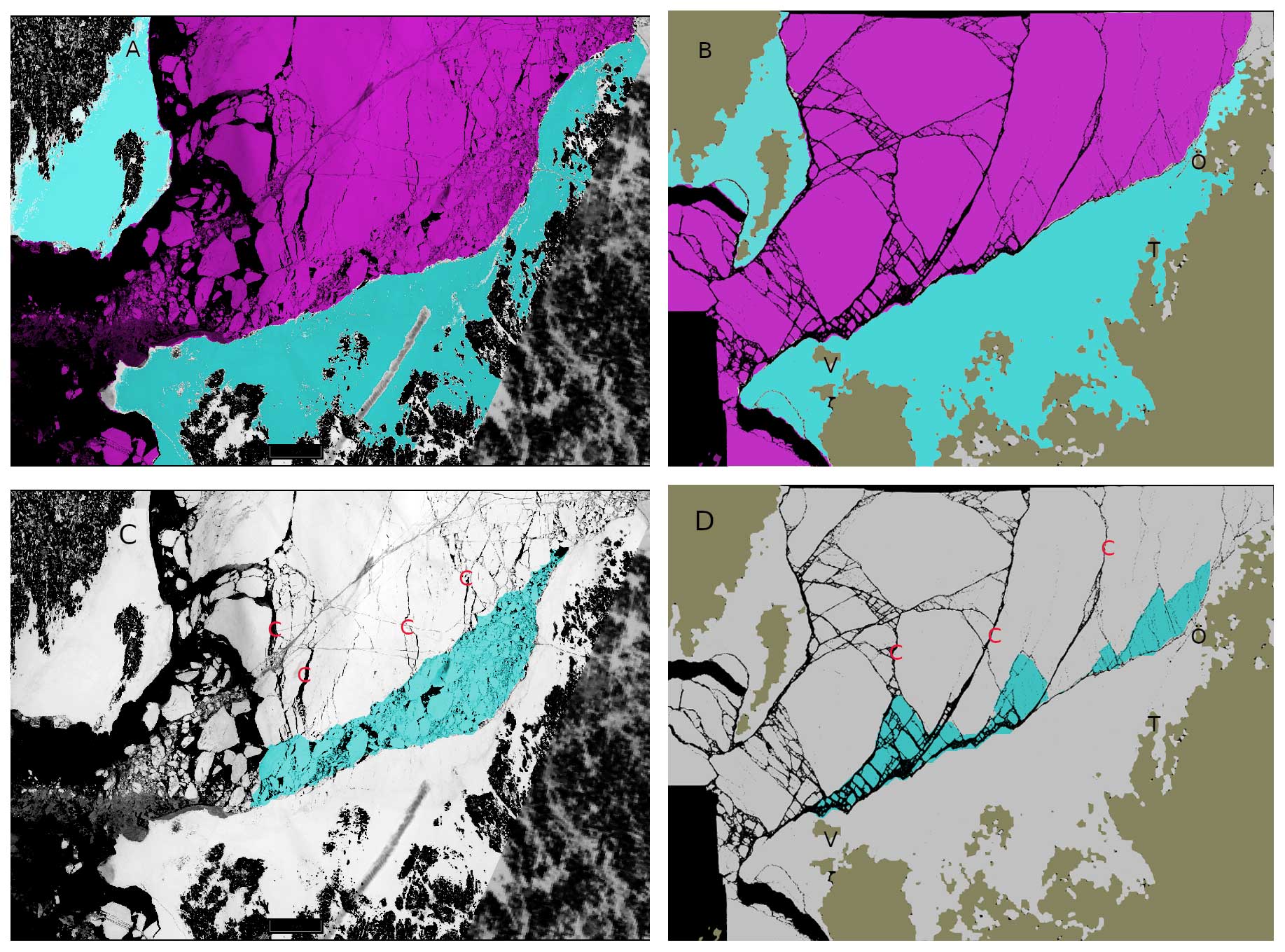
Figure 4 (a) Fast-ice regions (teal-blue) and drift ice regions (purple) extracted from the satellite image for 23 March 2018. (b) Fast-ice regions and drift ice regions at the end of the simulation. (c) Crushed-ice region and tensile cracks (marked by “C”) extracted from the satellite image. (d) Crushed-ice regions and tensile cracks at the end of the 23 March 2018 simulation.

3.2 Simulation case study for 8 March 2018

The other date for model testing in the Kvarken region is 8 March 2018. During a few days proceeding this day, there was a fairly constant, mostly eastern wind. We use the same initial state in this case as that used in the 23 March 2018 case, except that we now define two regions of stronger landfast ice to test how this influences the outcome of the simulations. One region of stronger ice is the strait between Holmön and the Swedish mainland, and the other region is the Finnish archipelago along the southern border of the domain terminating close to Valsörarna (marked by “V” in Fig. 4d). The effect this has is visible, for example, in Fig. 2b. The damaged ice breaks, while the fast ice remains solid. Another difference from the previous case is that now the wind stress forcing on DEs comes from the east and not the north, and the simulation is a bit shorter (3 h and 15 min instead of 3 h and 45 min).

Figure 5a displays ice motion, while Fig. 5b shows the largest compressive strains at the end of the simulation. Similarly to the 23 March 2018 case, ice is pushed through the Kvarken Strait, but now, because of a different wind stress direction, the ice comes more from the east than from the north. Compressive stress builds up northeast of the strait, as in the previous case; however, in this case, there is also a significant compressive fracture of ice against the Swedish coast (Fig. 5b). The ice begins to break up along an east–west corridor ending between the south end of Holmön and the Finnish archipelago. The same corridor of fragmented ice can be seen in the satellite image, but in this case, it reaches almost all the way to the Finnish coast. It is quite clear that the simulation would have to run longer for significant fragmentation to reach that far east, even though the ice forcing is slightly exaggerated in the simulations, as explained above.

Figure 5c displays a satellite image of the region on 8 March 2018. In contrast to the previous case, the simulation image rendered to mimic the observations now displays, as before, fractured beams in black so that they are the same color as open water, but on top of them, all intact compressed beams are rendered in light gray to mimic regions in the satellite image that may have densely packed drift ice and would therefore appear white or grayish. It is not possible to determine from the satellite image (Fig. 5c) if the regions near the Swedish coast, northeast of Holmön, consist of densely packed drift ice, fast ice, or a mix of both. This issue may have two explanations – either the crushing of ice cannot be detected in the satellite image as it does not expose dark open water or the wind forcing was set too strong in the simulations. The latter is consistent with the weak to moderate eastern winds during 6 to 8 March 2018. Inspecting satellite images from 6 and 7 March 2018 reveals that it took at least 3 d to form the east–west fragmentation corridor. With the current model configuration, it would take a lot of computational resources to execute simulations for such durations.

Figure 5e and f highlight the floes (teal blue) that are about to flow out through the Kvarken Strait. The same figures display the land and landfast ice on the eastern side of Kvarken as purple areas. The teal-blue areas display obvious similarities, and the eastern border between the drift ice and landfast ice, indicated by the boundary of the purple areas, are very similar for the observed and the simulated images. A dominant diagonal lead, marked by “Dia”, appears in both images. However, the exact locations of this lead differ a bit between the observed and the simulated images. Finally, there are cracks in both images, marked by “Arc”, that have the characteristic curved shape of cracks formed in regions with compression arches.

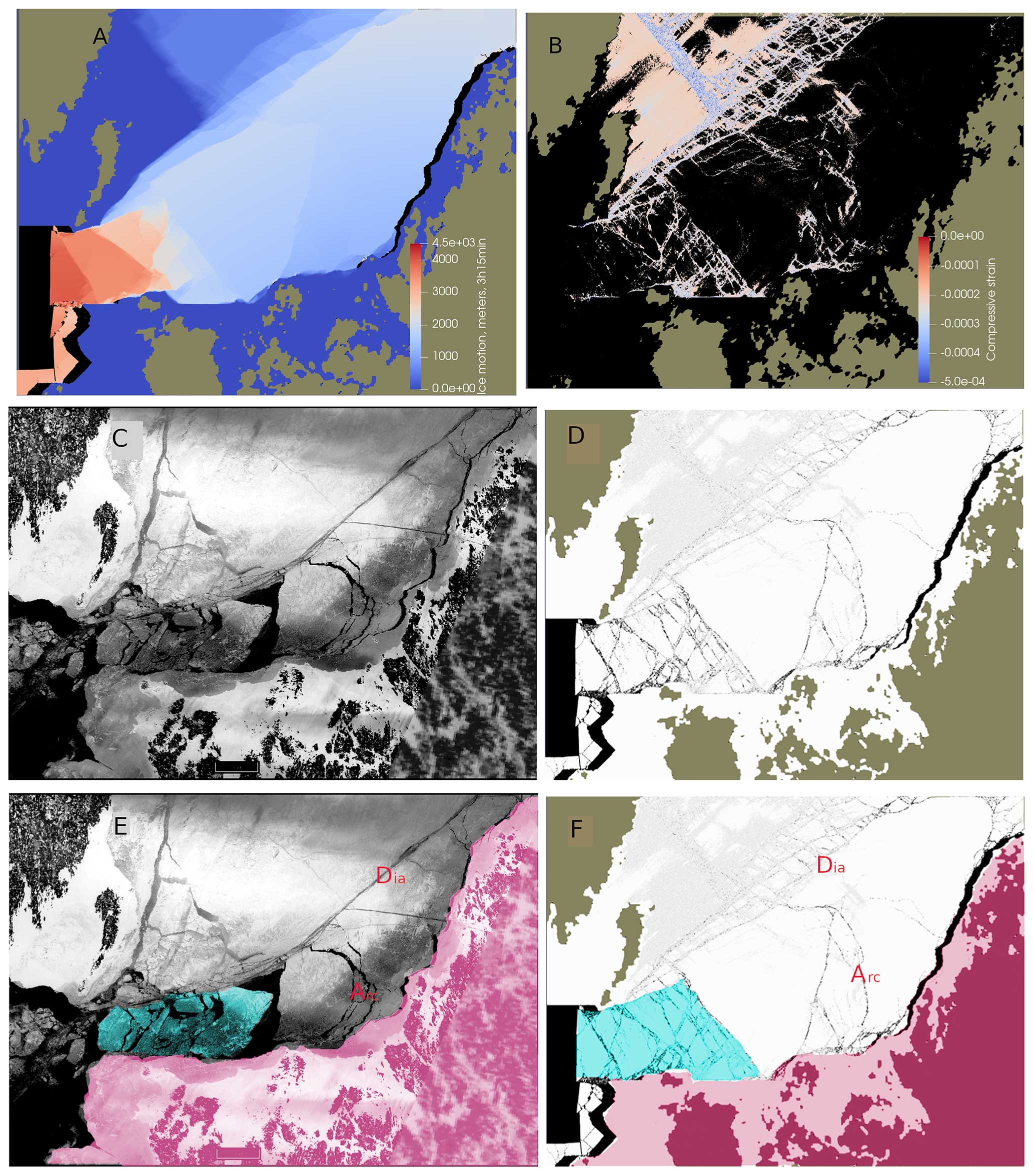
Figure 5 (a) Color-coded ice motion for the 8 March 2018 simulation. (b) The largest compressive strains on intact beams connecting DEs at the end of the simulation. (c) A satellite image of the Kvarken area on 8 March 2018. (d) The simulated fracture pattern after 3 h and 15 min. This image displays (with black dots) all beams that are strained to more than 5 % of their original length (and are thereby obviously broken) and displays (with light-gray dots) beams compressed by more than 0.02 % of their original length. (e) Drift ice that is on its way out through the Kvarken Strait (highlighted in teal blue). The purple area covers the land and landfast ice on the eastern (Finnish) side of Kvarken, highlighting the boundary between drift ice and fast ice. (f) The corresponding highlighted regions for the simulation. “Dia” marks the dominant diagonal lead, and “Arc” marks the cracks formed in regions with compression arches.

3.3 Floe size distributions

The floe size distribution (FSD) formed in the simulations may be extracted. We were not, however, able to extract the corresponding FSDs from the satellite images. Observed FSDs have recently been published with respect to the Canada Basin (Denton and Timmermans, 2022). They reported power-law FSDs, $n\left(s\right)\propto s^{-\mathit{\alpha }}$, with exponent α ranging from 1.65 to 2.03 over a floe area ranging from 50 m² to 5 km² and with larger exponent values appearing in the summer and fall as well as at low sea-ice concentration. Figure 6a and b display the FSDs from the 8 March 2018 and 23 March 2018 simulations, respectively. Power laws are evident with exponents 1.72 and 1.76, respectively. Also, the size ranges are similar to those reported by Denton and Timmermans (2022). However, the discreteness of the DEM becomes influential for the smallest floe sizes: a single element has an area of πr²≈50 m². As single DEs cannot be broken, there is a “pileup” effect in the FSDs for floes with a single or a few DEs. The largest “floes” in the FSDs, outside of the power-law range, represent the fast-ice regions.

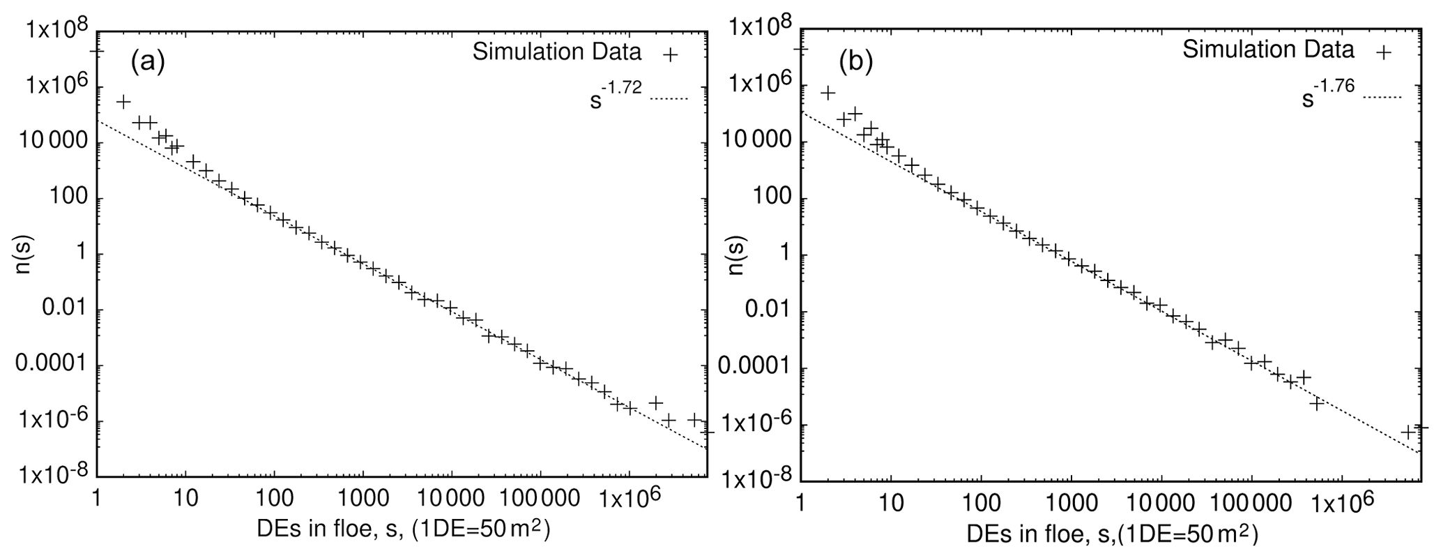
Figure 6 (a) The computed FSD at the end of the 8 March 2018 simulation fitted by power law with an exponent of 1.72. (b) The computed FSD at the end of the 23 March 2018 simulation fitted by power law with an exponent of 1.76. The scale on the x axis represents the number of DEs in a floe (1 DE ≈50 m²).

4 Gulf of Riga

An important characteristic of sea-ice compression is the formation of pressure ridges. In order to demonstrate how pressure ridges form in the HiDEM, a square-shaped sea-ice sheet measuring 10 km×10 km was modeled using DEs of 1 m diameter and subjected to uniaxial compression (Fig. 7a). Our simulation results may be assessed with the help of an aerial photograph of ice ridges in the Gulf of Bothnia from March 2011 (Fig. 7b). The dynamics process of ridge formation becomes rather evident in these two images. Compression, induced by a strong wind, breaks up the ice into floes. Along the floe boundaries, the ice fractures in compressive shear zones, and ice rubble builds up to form ridges. In the simulated image, the floes still remain largely in their original positions relative to each other, although they have moved enough to form patches of open water between them (Fig. 7b).

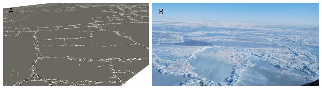
Figure 7 (a) A HiDEM simulation of the failure of a 10 km×10 km square-shaped sea-ice cover subjected to uniaxial compression. The sea-ice cover was modeled using a densely packed single layer of 1 m diameter spherical discrete elements. The sea-ice cover fails in shear, and ice ridges are formed. (b) An aerial photo taken at 30 m altitude showing fractured ice with pressure ridges in the Gulf of Bothnia after a storm in March 2011 (Jari Haapala, private photo).

Pressure ridge formation is a particular hinderance for shipping in the Baltic Sea. In the Gulf of Riga, ridges typically form under compression caused by southwestern winds. Such conditions are known to produce ridges, particularly between the Kihnu and Saaremaa islands. Figure 8a shows the strains between DEs that were initially connected by beams at the end of the simulation. Both intact and broken beams are included. Formed compression ridges appear in the figure as indistinct red bands of tension in an otherwise compressive ice landscape. Figure 8b shows the FSD extracted from the Gulf of Riga simulation. The exponent in this case is significantly larger (α≈2.12) compared to that in the Kvarken simulations. This is consistent with the topography of the Gulf of Riga, which (unlike the Kvarken Strait) does not allow the ice to flow out of the domain, and therefore, the ice floes are crushed and ground into smaller sizes (Sulak et al., 2017; Åström et al., 2021). The strain rate distribution can be extracted from the simulations. For the largest strains, the distribution of rates (Fig. 8c) is consistent with power-law distributions observed at much larger scales (Girard et al., 2009).

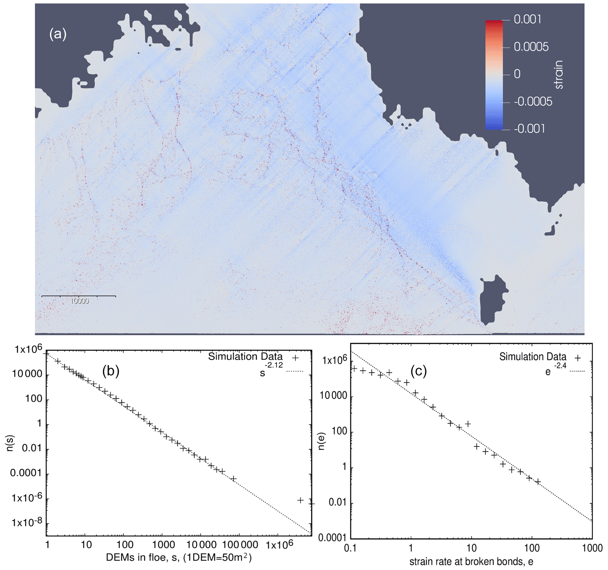
Figure 8 (a) Simulated strain field in the Gulf of Riga induced by southwestern winds. (b) FSD of the Gulf of Riga simulation. (c) Strain rate distribution, n(e), of the largest strains, e, in the Gulf of Riga simulation.

To further investigate ridge formation in the Gulf of Riga, we identify locations of compression ridges in the simulations as places where elements are pushed below the sea surface to form ridge keels. Ridges are affected by the bathymetry (Fig. 9a). It is evident from this figure that when long ridges are formed in a single event, like in our simulations, the structure of the ridges is strongly influenced by the shape of the coastline and the bathymetry in shallow waters where ridge keels begin to become grounded. It is, therefore, reasonable to expect that ridge patterns form fractals, just like coastlines and many structures formed by sea-ice dynamics do (Weiss, 2001). A simple box-counting algorithm, $N(L/l)\propto L/l^D$, can reveal the fractal dimension D. Here, $L/l$ is the linear number of boxes that the domain is divided into, and N is the number of boxes containing DEs identified as ridge keels. Figure 9b shows the result of this exercise, indicating that D≈1.12, which is a fairly low dimension. A dimension of D=1 would mean that ridges form nonfractal linear structures. It is reasonable to expect that if ridge fields were formed over longer periods and by different wind directions, they could eventually cover entire areas, and their dimension would then become D=2. The fractal dimension D=1.12 is a rather typical value for reasonably straight coastlines, such as those observed in the Gulf of Riga.

Figure 9c shows the locations of ice ridges observed from ice charts for 2000–2016. The ridge locations follow the general ridge pattern of the simulations reasonably well, indicated by the reddish area in Fig. 9c. Figure 9d shows the wind statistics (i.e., a wind rose) from the ERA5 data set (location: 58.00° N, 23.75° E) for the same time period (15 December to 1 May in 2000–2016). This figure demonstrates that ridges are predominantly caused by SW winds, with SW being the dominant direction of strong winds in the area.

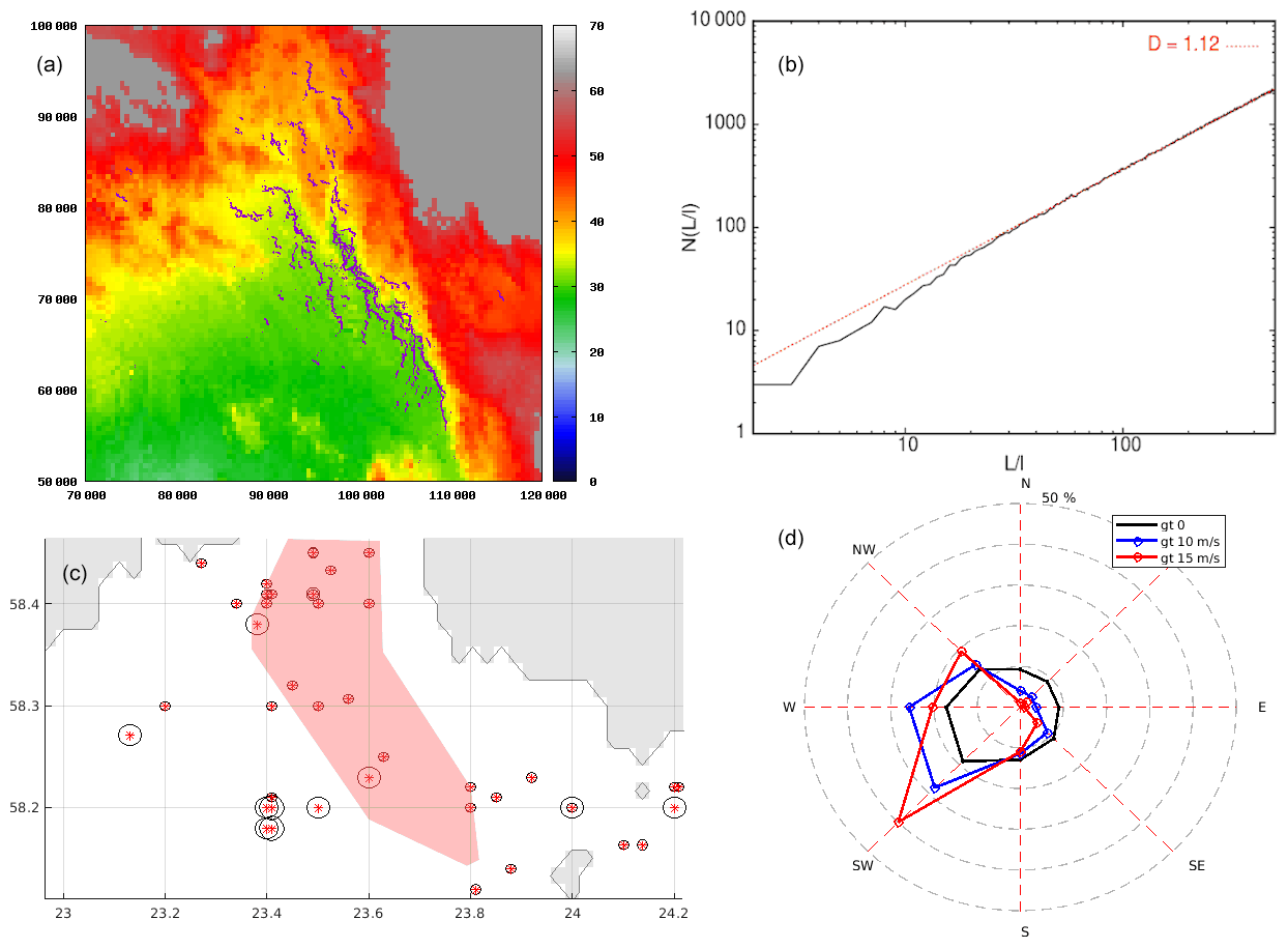
Figure 9 (a) Color-coded bathymetry. The water surface is at 57 m. The locations of DEs that make up compression ridges are indicated by blue markers. Single DEs on the surface would become grounded in dark-red areas. Gray areas represent land. The scale on the axes is given in meters. (b) The result of a box-counting algorithm for compression ridges, $N(L/l)\propto L/l^D$, where l is box length, L is domain length, and N is the number of boxes containing ridges. (c) Observed locations (lat, long) of ridges from ice charts. The statistics are based on the data from winters in 2000–2016 (15 December–1 May). Red stars indicate ridge locations, and the diameter of each black circle indicates the number of days of ridged-ice presence at that location. The reddish region indicates the area where ridges form in the simulations. (d) A wind rose showing wind speeds greater than 0, 10, and 15 m s⁻¹ for 15 December to 1 May (2000–2016). The dashed lines indicate frequency intervals of 10 %.

5 Discussion

The outcomes presented, along with prior findings on ice shelf disintegration (Benn et al., 2022), laboratory-scale ice-crushing experiments (Prasanna et al., 2022), and glacier calving (Åström et al., 2021), illustrate that the HiDEM has the capability to model the physics of ice fragmentation. In practical terms, the current version of the code can be utilized to forecast sea-ice movement and fragmentation for a few days across distances of a few hundred kilometers. However, ensuring a consistent supply of accurate forecasts would necessitate a method for acquiring high-quality initial conditions. This would require a comprehensive understanding of variations not only in ice thickness but also in ice quality. Additionally, accounting for spatial variations in ice surface roughness is crucial as it impacts the local stress on ice induced by winds and currents. Moreover, precise forecasts of winds and currents would be essential to determine the forces acting on the ice during simulations. Proper boundary conditions would also need to be established for each scenario, especially if the ice is permitted to exit the simulation domain. While evaluating this in cases where the domain is bounded by land is straightforward, it becomes more challenging when the boundary crosses water with dynamic ice both inside and outside the domain. Enhancing the HiDEM code for sea-ice forecasts would significantly benefit from improved comparisons with quantitative observational data on sea-ice dynamics that could be directly juxtaposed with simulation data for any specific location. For instance, having detailed data on the evolving floe size distribution, shapes, and locations in the Kvarken Strait for a specific time frame would be highly valuable for further validating the HiDEM. Similarly, recording the formation of compression ridges and ice motion in the Gulf of Riga, such as during a midwinter storm with southwest winds, would be equally beneficial. Any observed distribution function, velocity field, or stress field of this nature could be valuable for comparison with simulation results, provided that the simulation starts with precise initial conditions and that the simulated ice dynamics are driven by valid forces.

One challenge is the disparity between the short time step required for accurate fracture dynamics and the relevant timescales for sea-ice dynamics. The time resolution, dt, must be smaller than the time it takes for sound to travel across a DE, which for ice translates to $\mathrm{d}t<{\mathrm{DE}}_{\mathrm{diameter}}/\sqrt{K+\mathrm{3}G/\mathrm{4}}\approx \mathrm{0.0025}$ s (for the setup used in this investigation). K represents the bulk modulus, and G represents the shear modulus for ice. Here, a time step of dt=0.001 s has been used. This implies that 3.6 million time steps are necessary to simulate 1 h of ice dynamics. Even with the highly optimized HiDEM code, practical simulation times are typically constrained to a range from a few hours to several tens of hours, depending on the available computational resources. In contrast, the relevant timescale for sea-ice dynamics may span days, weeks, or months. Although it is feasible to accelerate ice dynamics slightly in simulations compared to natural rates, the limitation in simulation times means that it is not feasible to compute entire winter seasons of sea-ice dynamics. Instead, a snapshot of sea ice at a specific time must be generated based on observations, and the near-future ice dynamics can then be simulated from such a starting point.

It is important to note that the HiDEM code solely models sea-ice dynamics as elastic–brittle fracture and dynamics, omitting the thermodynamic processes involved in sea-ice formation and disintegration. Over extended periods and in extreme temperature conditions, thermodynamic processes often dominate sea-ice behavior, while in shorter time frames in which ice is subjected to stresses surpassing its strength, elastic–brittle behavior typically prevails. A potential approach to encompass the full spectrum of processes would be to integrate a code like the HiDEM with a large-scale continuum model that includes the modeling of thermodynamic processes.

The ice breakup events in Kvarken in March 2018, as detailed in this report, were accompanied by air temperatures hovering around −10 °C, indicating the possibility of new ice formation. Nevertheless, the influence of the windy weather conditions would have constrained freezing rather effectively during the time frame of a few dozen hours that is pertinent to the modeled and observed elastic–brittle breakup.

6 Conclusions

In this study, we utilized the HiDEM to analyze sea-ice fragmentation and have shown its capability to accurately replicate observed characteristics. Specifically, we compared the outcomes of the simulations with satellite imagery from the Kvarken area of the Baltic Sea from March 2018. The external forces acting on the ice in the simulations were derived from weather archives. The fracturing of the ice and its movement through the narrow Kvarken Strait were primarily influenced by moderate to strong winds blowing from the north and east. Despite using an 8 m grid resolution, minimal model adjustments, and basic initial conditions, the model successfully replicated a significant portion of the fracture patterns, fast-ice distributions, and ice drift patterns observed in the satellite images. Furthermore, we explored the formation of compression ridges in the Gulf of Riga and discovered that the size distributions of floes and the development of compression ridges aligned well with real-world observations. While the model offers detailed insights into fracture patterns, leads, compression ridges, and floes, its practical utility as a forecasting tool is constrained by certain limitations. The model's ability to simulate at a high resolution is restricted to relatively small domains, and the duration of the simulated ice dynamics is also constrained. The most favorable method for improving the precision of ice dynamics predictions seems to be a blend of DEM and continuum models, as these two model types possess contrasting strengths and weaknesses.