the Creative Commons Attribution 4.0 License.
the Creative Commons Attribution 4.0 License.
 | 03 May 2024
Understanding the drivers of near-surface winds in Adélie Land, East Antarctica
Cécile Davrinche
Anaïs Orsi
Cécile Agosta
Charles Amory
Christoph Kittel
Near-surface winds play a crucial role in the climate of Antarctica, but accurately quantifying and understanding their drivers is complex. They result from the contribution of two distinct families of drivers: the large-scale pressure gradient and surface-induced pressure gradients known as katabatic and thermal wind. The extrapolation of vertical potential temperature above the boundary layer down to the surface enables us to separate and quantify the contribution of these different pressure gradients in the momentum budget equations. Using this method applied to outputs of the regional atmospheric model MAR at a 3-hourly resolution, we find that the seasonal and spatial variability in near-surface winds in Adélie Land is dominated by surface processes. On the other hand, high-frequency temporal variability (3-hourly) is mainly controlled by large-scale variability everywhere in Antarctica, except on the coast. In coastal regions, although the katabatic acceleration surpasses all other accelerations in magnitude, none of the katabatic or large-scale accelerations can be identified as the single primary driver of near-surface wind variability. The angle between the large-scale acceleration and the surface slope is a key factor in explaining strong wind speed events: the highest-wind-speed events happen when the katabatic and large-scale forcing are aligned, although each acceleration, when acting alone, can also cause strong wind speed. This study underlines the complexity of the drivers of Antarctic surface winds and the value of the momentum budget decomposition to identify drivers at different spatial and temporal scales.
- Article
(9370 KB) - Full-text XML
-
Supplement
(7513 KB) - BibTeX
- EndNote


Near-surface winds play a key role in the Antarctic climate system. First, they contribute to an active mass exchange between the continent and sub-polar latitudes. They transport cold surface air northward, which causes warmer subpolar air masses to rise and travel southward to replenish the cold air removed (Parish and Bromwich, 1998). Moreover, they have a major influence on the ice sheet surface mass balance. At the surface, they redistribute surface snow across the continent, which can sublimate during transport in the lower atmosphere (Lenaerts et al., 2012; Amory et al., 2021; Gerber et al., 2023). Additionally, high near-surface wind speeds enhance the mass and energy exchange at the surface–atmosphere interface and contribute to increase the sublimation of surface snow (Bintanja, 1998). Furthermore, near-surface winds originating from the cold and dry inner continent supply the lower troposphere with unsaturated air as they flow downslope and adiabatically warm up (Gallée and Pettré, 1998). This causes precipitating snow to sublimate into the atmosphere (Vignon et al., 2019; Jullien et al., 2020) and thus decreases the amount of precipitation reaching the ground by up to 35 % on the margins of East Antarctica (Grazioli et al., 2017).
These winds are complex because they result from two different families of drivers: in the free atmosphere, winds are governed by large-scale pressure gradients. Additionally, in the boundary layer, the dense, cold surface air, caused by surface net radiative cooling (followed by turbulent sensible heat exchange between the atmosphere and the surface), is accelerated by gravity on the steep surface slope, generating a divergent flow called katabatic wind (Gallée and Pettré, 1998). At the same time, the accumulation of cold air over the lowest part of the slope and the sea ice induces a poleward flow, the thermal wind, which opposes the katabatic flow near the foot of the slope (Vihma et al., 2011).
It is important to disentangle the impact of large-scale and boundary layer forcings on Antarctic near-surface winds because they have different drivers and might evolve differently in the future. In the next decades, during winter, the large-scale forcing is expected to weaken at the ice sheet ocean margins due to a more positive southern annular mode (SAM) (Hazel and Stewart, 2019; Neme et al., 2022).
Simultaneously, the katabatic forcing could also decrease in a warmer climate due to the increase in downward longwave radiation. However, the decrease in boundary layer stability might also induce stronger mixing with upper-geostrophic winds by increased vertical momentum transfer (Bintanja et al., 2014). The resulting change in wind speed is thus very uncertain and depends greatly on the region of Antarctica, with potential cancellation between regions of increase and decrease (Bracegirdle et al., 2008).
In order to study the temporal variability in Antarctic near-surface winds, it is thus essential to look at each component of the momentum budget separately. In previous studies, the katabatic nature of Antarctic near-surface wind forcing diagnosed using the directional constancy has been overemphasized. It had been suggested that the katabatic nature of winds could be estimated using Weibull shape parameters (Sanz Rodrigo et al., 2013) like in Greenland (Gorter et al., 2014). However, in Antarctica, the large-scale pressure gradient is also directed from the interior to the coast, which has led to an overestimation of the role of the katabatic forcing for decades (Parish and Cassano, 2003). Instead, a full decomposition of the momentum budget with separation of large-scale and boundary layer contributions is necessary.
The momentum budget decomposition has proven to be a useful tool to study the spatial variability in the different acceleration terms for modelled monthly averaged wind fields (van den Broeke and van Lipzig, 2003; Parish and Cassano, 2001). Fewer studies have focused on understanding the variability in these winds on sub-daily to monthly timescales. Yasunari and Kodama (1993) tackled this aspect, albeit at a 30 m level and focusing only on periods ranging from 30 to 60 d. Unfortunately, this range excludes the analysis of short events such as high-wind-speed events which typically last for less than 2 d. Renfrew and Anderson (2002) conducted case studies at a 3-hourly resolution using automatic weather station (AWS) data but had to assume the katabatic nature of winds due to the lack of vertical depiction of the atmosphere.
Here we identify the drivers of the temporal variability in near-surface winds by computing the momentum budget in the atmosphere at a 3-hourly resolution, with a regional focus on Adélie Land in East Antarctica. Compared to previous approaches, our study focuses on understanding the variability in the near-surface winds (7 m above ground level) for a larger range of timescales using a more accurate diagnosis obtained through an extensive analysis of the vertical profiles of the atmosphere, using the polar-oriented regional atmospheric model MAR. We first quantify the dominant components of the momentum budget by analysing the spatial and seasonal variations in each term in the momentum budget. Then, we focus on the correlations between the different acceleration terms and the total wind speed at a 3-hourly resolution.
2.1 Data
2.1.1 Field observations over a transect in Adélie Land
We focus on the East Antarctic region located between coastal Adélie Land and the Antarctic Plateau (Fig. 1), taking advantage of the supply route between Dumont d'Urville station (DDU; 66.7° S, 139.8° E; 0 m above sea level) and Concordia station, Dome C (DC; 75.1° S, 123.3° E; 3233 m a.s.l.). This transect is typical of the climatology of Antarctica, with downslope flow from the East Antarctic Plateau to the coast and strong easterlies along the coast. Coastal Adélie Land is known for its very strong near-surface winds, with the highest wind speed recorded in Antarctica (96 m s−1) monitored at DDU in the late 1970s (Wendler, 1990), which makes it an ideal area to study the drivers of near-surface wind variability.
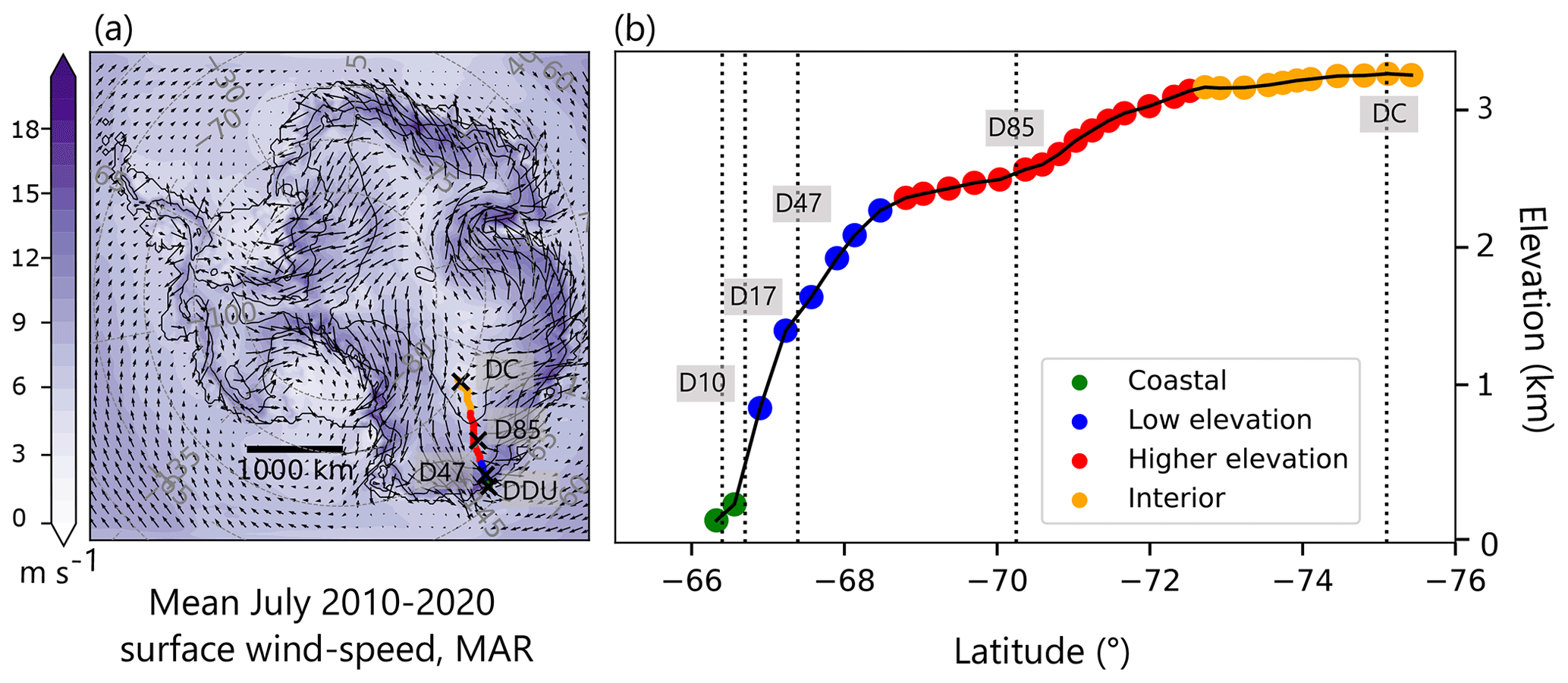
Figure 1(a) Map of average July 2010–2020 norm of near-surface wind speed (MAR). Superimposed are the mean vectors. Solid black lines are for elevation contours every 500 m (a.s.l.). The transect is indicated in coloured dots. Four weather stations are indicated: D10, D47, D85, and Dome C (DC). Dumont d'Urville (DDU) is located 5 km offshore of D10 and 34 km of D17. (b) Elevation profile along the transect extracted on the 35 km MAR grid. For both plots, colour dots represent the different sectors detailed at Table 2, with green dots on coastal area, blue dots on lower elevations, red dots on high elevations, and orange dots on the Antarctic Plateau. The spacing of the dots is related to the MAR grid.
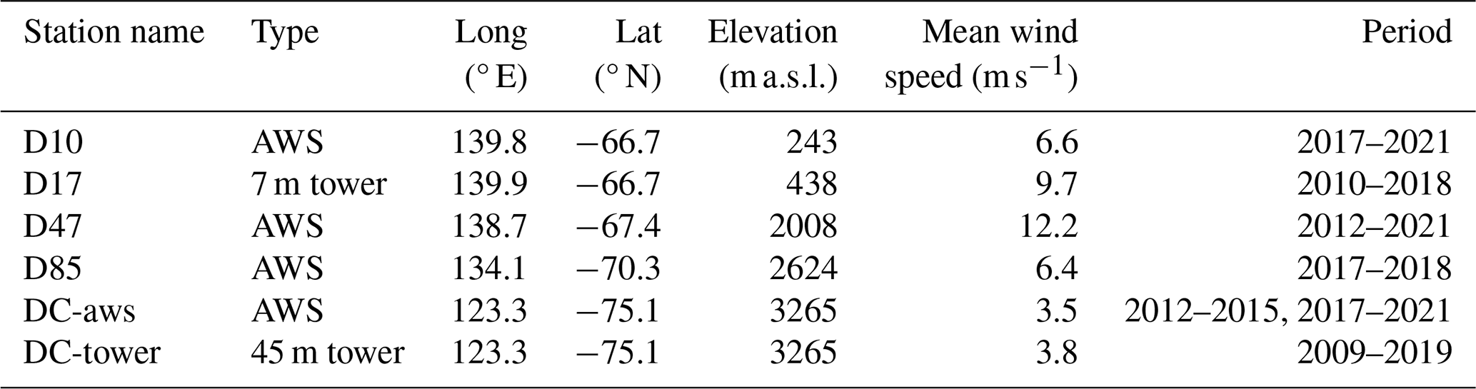
This supply route is well instrumented, with six weather stations described in Table 1 and shown in Fig. 1. The wind speed recorded in each of these six stations enables us to assess the model's ability to represent the winds in a wide range of conditions. Four automatic weather stations (AWS, 2010) record temperature and wind speed at approximately 2 m above ground level (a.g.l.), with data provided at a 3-hourly resolution. Additionally we use 3-hourly quality-controlled wind speed from two weather profiling towers: the first level (≈ 2 m) of a 7 m tower at D17 (Amory et al., 2017, D17, CALVA project) and the first level (≈ 3 m) of a 45 m “American tower” at DC (Genthon et al., 2021). All these observations are available even during wintertime, when wind speeds are particularly high (seasonal maximum) and the diurnal cycle is very weak (polar night), leading to favourable katabatic conditions. In the following, we will focus more specifically on the months of July 2010–2020: July is the month of the year when the wind speed is highest and also free of the radiative forcing due to the diurnal cycle of insolation.
2.1.2 Regional atmospheric model
Our goal is to disentangle the contributions of large-scale and boundary layer drivers in shaping the near-surface winds of Antarctica. In order to do this, we need a description of the vertical atmospheric column, which is only available in radiosoundings at the two extremities of our transect, DDU and DC. Consequently, due to the scarcity of observations, we perform our study using outputs from the regional atmospheric model MAR v3.11 for the period 2010–2020 (https://gitlab.com/Mar-Group/MARv3, last access: 24 April 2024), after evaluation of this model for near-surface winds (Sect. 3.1). MAR is a regional hydrostatic model that takes into account specific physical properties of the Antarctic region, in particular a multi-layer snow model based on CROCUS (Brun et al., 1992; Vionnet et al., 2012), with several adaptations for Antarctica, including meltwater refreezing and parameterized fresh snow density (Agosta et al., 2019). Topography, ice mask, and rock mask are derived from Fretwell et al. (2013). The equations of the atmospheric model, lateral boundary, upper- and lower-boundary conditions, and the main parameterizations are extensively described in Gallée and Schayes (1994), and a description of the adaptation of MAR to the Antarctic ice sheet can be found in Agosta et al. (2019) and Kittel et al. (2021). Relative to previous studies over the Antarctic ice sheet (Agosta et al., 2019), the version used in this study improves the cloud lifetime, the model stability and its computational efficiency, and the inclusion of rock outcrops, as in Mottram et al. (2020) and Kittel et al. (2021). In addition, MAR v3.11 includes a correction of the cloud microphysics in the upper relaxation zone, where clouds were set to zero in previous versions of the model (Kittel et al., 2021). We increased the snow albedo by 5 % (relative to the previous value) in agreement with recent model evaluations performed at DC.
We use 3-hourly outputs of MAR v3.11 with 24 vertical atmospheric levels (first model level ∼ 2 m a.g.l.), 30 snow or ice layers distributed over a fixed 20 m thickness, and a horizontal resolution of 35 km. MAR is forced with 6-hourly outputs of the ERA5 reanalysis (Hersbach et al., 2020) at its lateral boundaries (temperature, wind, humidity) and for upper-air relaxation at the top of the troposphere (temperature, wind), as well as with daily outputs at the surface of the ocean (sea surface temperature, sea ice concentration).
2.1.3 Coast-to-plateau transect on the model grid
The spatial variability in near-surface winds is strongly linked to the topography of Antarctica with the strongest winds just under the steepest slopes. The supply route between DDU and DC crosses a wide range of slopes, which enables us to study the various wind drivers, in particular the katabatic acceleration. On the 35 km MAR grid, we extract the DDU–DC transect by following the steepest slope trajectory upstream and downstream of D47. This transect reaches an upstream location close to DC and a downstream location close to DDU station (Fig. 1). We divide the transect into four elevation bins with different slopes, similar to van den Broeke et al. (2002), which are detailed in Table 2 and shown in Fig. 1: a coastal region at the foot of the slope (0–100 m a.s.l.), a low-elevation region with steep slopes (100–2300 m a.s.l.), a higher-elevation region with gentler slopes (2300–3100 m a.s.l.), and the nearly flat plateau (3100–3300 m a.s.l.). By construction, the transect follows the steepest slope direction, which enables us to capture the spatial variability in wind from its formation on the plateau to its acceleration along the slopes of Adélie Land and up to the coastal area.
Table 2Characteristics of regions defined along the study transect on the 35 km MAR grid. Transect location is shown in Fig. 1.
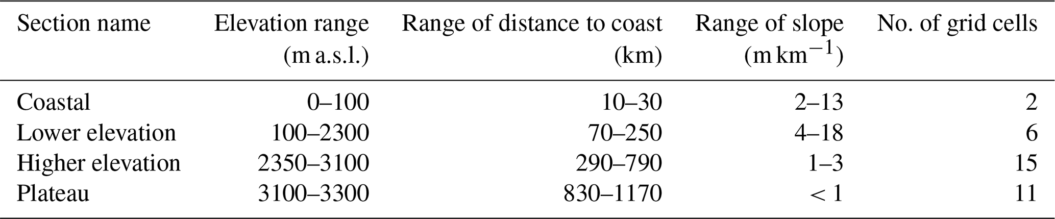
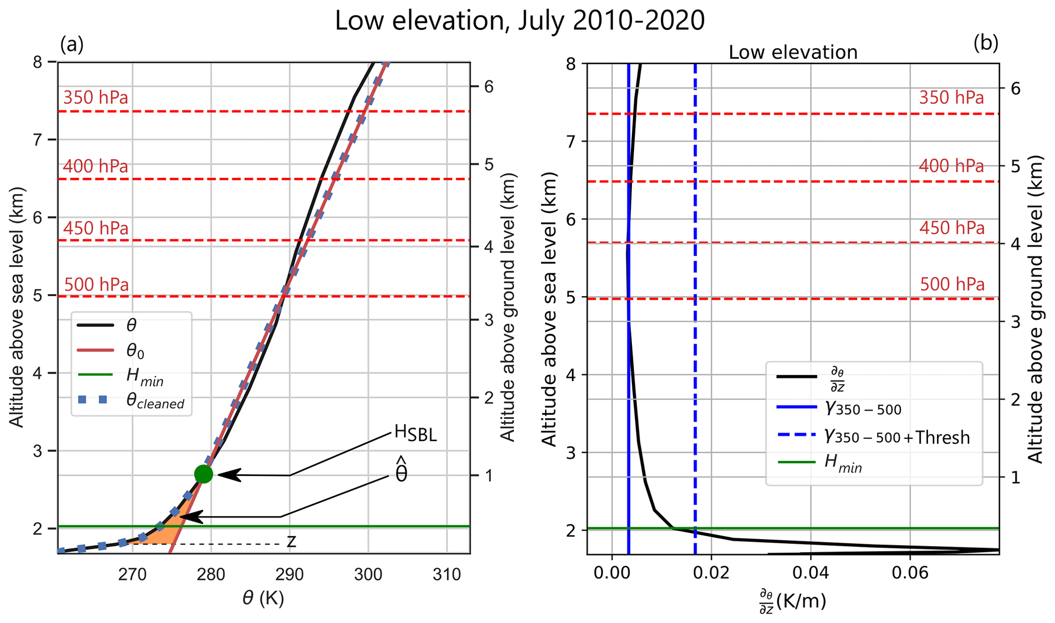
Figure 2Schematic defining variables used for separation of large-scale and surface forcings. (a) Typical vertical profile of potential temperature θ computed for July 2010–2020 at low elevation (120–2300 m a.s.l.) on the transect (solid black line). Solid red line represents the linear background potential temperature θ0, which is a linear interpolation of θ between 350 hPa and the altitude Hmin (solid green line). The dotted blue line indicates the correction performed on θ to avoid positive values of the potential temperature deficit above HSBL (green dot), which is the lowest altitude for which Δθ becomes positive. (b) Typical profile of the vertical derivative of potential temperature (, black line) computed for July 2010–2020 at low elevation (120–2300 m a.s.l.) on the transect. The solid blue line represents the mean value of computed between 350 and 500 hPa. The dotted blue line indicates the threshold value of 5 below which we consider the vertical potential temperature profile to be no longer quasi-linear. Hmin is defined as the maximum height under which .
2.2 Method
2.2.1 Separation of large-scale and surface forcings in the vertical potential temperature profile
The goal of this study is to separate the main drivers of near-surface wind variability. Near-surface winds are the result of two types of forcing: the large-scale pressure gradient and the additional pressure gradients associated with the vicinity of the surface. It was shown by van den Broeke and van Lipzig (2003) that we can separate the pressure gradient force (PGF) into the contribution of surface and large-scale pressure gradients using the potential temperature. The vertical potential temperature profile in the free troposphere (i.e. above the boundary layer and below the tropopause) is approximately linear (see Fig. 2a). Well above the boundary layer (typically above 500 hPa), the potential temperature is only influenced by large-scale pressure gradients. Thus, we linearize the potential temperature above the boundary layer and extrapolate it to the surface:
with z the altitude a.g.l., γ0 the vertical gradient of the background potential temperature in the free atmosphere (in K m−1), and τ0 the intercept of θ0 at ground level (in K). We interpret θ0 as the background potential temperature, linked exclusively to the large-scale forcing. On the other hand, the difference between the real potential temperature profile θ and the background temperature θ0 (called the temperature deficit, ) is associated with the surface processes such as katabatic and thermal wind, defined later.
These definitions are based on the hypothesis that we can define for each grid cell and each time step a minimum height Hmin above which the vertical profile of θ is quasi-linear and the free atmosphere is not influenced by surface processes. In other words, above Hmin, the vertical derivative of potential temperature should be equal to a quasi-constant value, and Hmin is defined as the height below which the vertical derivative of potential temperature deviates from this quasi-constant value. The challenge related to the definition of the background potential temperature θ0 is to be able to accurately define this lowest altitude Hmin on which to interpolate the potential temperature. Should we take it too low or too high, we would wrongly interpret pressure gradients associated with large-scale processes.
We are confident that pressure levels between 500 and 350 hPa fall within the free troposphere in Antarctica, as the tropopause is typically between 150 and 320 hPa in this region (Hoffmann and Spang, 2022). Therefore, the slope of the linear interpolation of θ between 500 and 350 hPa (γ350−500) gives a good first estimate of γ0. In order to fine-tune γ0, we look for the minimum height Hmin under which the vertical derivative of potential temperature computed at each level deviates from γ350−500. We do so by finding the height Hmin for which , with Thresh a threshold on the first vertical derivative that we need to define (Fig. 2b).
A first option would be to determine a constant threshold in time and space. However we realized that for vertical profiles with a high γ350−500, the threshold needed to be higher than for smaller γ350−500. Therefore we decided to chose a threshold proportional to γ350−500:
A sensitivity study of the coefficient N is provided in Fig. S2 of the Supplement. It is also possible to define a threshold on the second-order vertical derivative instead of on the first derivative of potential temperature to determine Hmin. Figures S3 and S4 provide a comparison of these methods at D47 for July 2018 and show that both methods are equivalent.
We also force Hmin to be greater than 100 m a.g.l., as we assume surface processes to always play a role below this height. Once Hmin is determined, we compute θ0 as the linear interpolation of θ between Hmin and 350 hPa, which gives an estimate of γ0 and of τ0 for each 3-hourly time step and each grid cell. Finally, we apply a spatial smoothing function (Gaussian filter) to γ0 and τ0 to obtain a horizontally smooth θ0, required for the horizontal derivative (see Eq. S25 in the Supplement) in the large-scale wind computation described in Eqs. (6) and (7). This is a reasonable assumption, since the large-scale potential temperature field does not change abruptly. As Δθ is the potential temperature deficit in the boundary layer, it must be negative by definition. However, the interpolation line θ0 always crosses θ. We look for the lowest altitude HSBL (see green dot in Fig. 2) for which Δθ becomes positive, and we force Δθ to be equal to 0 above this altitude (see dotted blue line in Fig. 2a). This approximation is justified in Sect. 3.2.
2.2.2 Momentum budget decomposition
We use the decomposition of the vertical potential temperature profile to separate the contribution of surface and large-scale pressure gradients in the momentum budget equations. As the wind follows the Antarctic topography at the surface of the ice sheet, we use the momentum budget equations in a coordinate system related to the topography (x, y, z), where (x, y) is the plane following the surface slope of the topography, with y being the downslope direction and z being the vertical axis normal to the surface slope, as in van den Broeke et al. (2002):
| Horizontal | Coriolis | Vertical advection | Large-scale | Thermal wind | Katabatic | ||
| advection | and turbulence | ||||||
| Cross-slope: | ADVH | COR | TURB | LSC | THWDTD | KAT | |
| +fV | −fVLSC | (3) | |||||
| Downslope: | |||||||
| −fU | +fULSC |
with
The derivatives with respect to time of the cross-slope wind U (in m s−1) and the downslope wind V (in m s−1) are decomposed into six accelerations: the horizontal advection (ADVH); the Coriolis deviation (COR); the large-scale acceleration (LSC); the thermal-wind acceleration related to the potential temperature deficit (THWDTD); the katabatic acceleration (KAT); and a residual term that includes the vertical advection, drag, and turbulence (TURB) in m s−1 h−1. A detailed description of the derivation of these equations is given in the Supplement (Sect. S2.2). The Coriolis factor f is equal to (λ), with Ω the rotation rate of the earth in s−1 and λ the latitude. The katabatic acceleration is computed using the potential temperature deficit Δθ defined in Sect. 2.2.1 and illustrated in Fig. 2. This is a classic definition documented in Ball (1956) and Mahrt (1982). For the altitude z (a.g.l.), if z>HSBL, then θ=θ0 (as detailed in Sect. 2.2.1). In the following, we will also use a constant zmax=z450 hPa, an arbitrary height that verifies everywhere so that we can compute the integration in Eq. (5) with constant bounds.
The thermal-wind acceleration (THWDTD) is a function of the horizontal gradients of , the vertically integrated potential temperature deficit between the ground, and zmax (Eq. 5 and Fig. 2). Note that the classic definition of thermal wind does not include a vertically integrated gradient of potential temperature deficit but of potential temperature. Here, we use the definition of van den Broeke and van Lipzig (2003), while Parish and Cassano (2003) named this term “integrated deficit”. It causes a surface flow from areas of weak to large negative values of , similarly to a sea-breeze circulation.
The large-scale acceleration is defined as the geostrophic acceleration in equilibrium with the background potential temperature profile (van den Broeke and van Lipzig, 2003):
where p is the pressure in Pa, and Rd and Cp are respectively the gas constant and specific heat capacity of dry air (Rd=287 and Cp=1005.7 ). The vertical large-scale wind gradients with respect to pressure and are then integrated between z and zmax. At zmax, none of the surface-influenced processes are at stake. Thus, the turbulence and katabatic and thermal-wind accelerations all equal zero. In Antarctica, this happens around 3000 m above ground level.
Consequently, at the level z=zmax, we obtain the following from Eqs. (6) and (7):
ULSC(z) and VLSC(z) are then computed by the integration of Eqs. (6) and (7), downward from zmax.
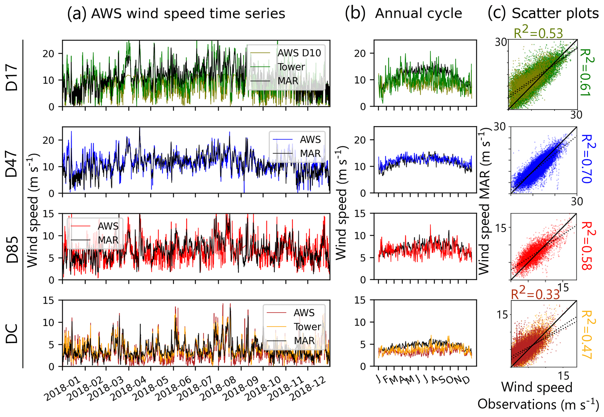
Figure 3From top to bottom D17, D47, D85, and Dome C. (a) Comparison of 3-hourly MAR outputs (black lines) with meteorological tower measurements (when available, i.e. at DC and D17/D10) and AWS (coloured lines). (b) Seasonal cycle computed for the years available at each AWS (see Table 1), with MAR, AWS, and the meteorological towers. (c) Scatter plots comparing observations and model outputs for each station. Solid black lines indicate the y=x line, while the dotted ones are the linear fit associated with each evaluations. The determination coefficient R2 is indicated next to each scatterplot.
3.1 Evaluation of MAR winds on the transect
Overall, in our simulations, MAR is able to capture the temporal variability in near-surface winds at a 3-hourly frequency reasonably well (Fig. 3a). This includes a good representation of the spatial differences in the seasonal cycle (Fig. 3b), which is more pronounced in locations closer to the coast, such as D17 and D47, than in the interior. The model underestimates slightly the mean 2 m wind speed at D47 with a bias of −0.6 m s−1. However, across all the other stations, the model tends to overestimate the mean wind speed with a bias ranging from 0.6 m s−1 for D85 to 2.0 m s−1 at D17. The largest biases are found during winter time at D17 and DC, with an overestimation of the seasonal cycle in MAR, compared to AWS measurements of about 60 % in D17 and 90 % in DC. The strongest correlations are found at sites with higher mean wind speeds such as D47 (R2=0.7) and D17 (R2=0.61) (Fig. 3c).
At the coast, the D10 AWS (≈ 3 km from the coast) and D17 weather profiling tower (≈ 10 km from the coast) are contained within the same MAR grid cell, whose centre is equidistant from both stations. MAR correlates slightly better with the observations from D17 (R=0.61) than from D10 (R=0.53), and both stations are well correlated (R=0.87). This may be due to the fact the model grid cell is more representative of continental than oceanic conditions. The two wind sensors of the American tower and the AWS at Dome C are also located within the same MAR grid cell. Although it has been demonstrated that the AWS temperature was biased because the instruments were not ventilated (Genthon et al., 2010), there has been no assessment of the comparative performance of the wind measurements.
MAR biases at D17 and DC may result from its turbulence scheme. Turbulence in the atmospheric boundary layer is parameterized using a local E−ε scheme adapted to stable atmospheric boundary layers in which small eddies develop and dissipate rapidly (Amory et al., 2015). Local turbulence schemes, however, commonly fail to represent the downward entrainment of momentum by large eddies of greater vertical extent (Hillebrandt and Kupka, 2009). This typically happens in well-mixed atmospheric boundary layers, as encountered in coastal Adélie Land during strong winds (Amory et al., 2017). The resulting misrepresentation of wind speed maxima is partly compensated for by a temperature-dependent parameterization for z0, which has been tuned to better capture observed wind speed maxima (at the expense of minima) and seasonal variations in wind speed in coastal Adélie Land (Amory et al., 2021).
3.2 Evaluation of the momentum budget decomposition (MBD)
The momentum budget decomposition (MBD) performs a separation between the accelerations of the wind induced by large-scale acceleration (LSC) that are the only drivers above the boundary layer and the accelerations of the wind resulting from surface forcings (i.e. katabatic (KAT), thermal wind (THWDTD), and turbulence (TURB)), which are zero above the boundary layer and are intensified near the surface. LSC is computed using the background potential temperature θ0, while surface processes are computed using the potential temperature deficit Δθ for KAT and the integrated potential temperature deficit for THWDTD. As a first evaluation step, we verify that this is indeed the case by plotting vertical profiles of each acceleration of the wind (Fig. S11) and of the different metrics (θ, θ0, Δθ, ) computed during our separation of the vertical potential temperature on the transect (Fig. 4): the katabatic acceleration is proportional to Δθ, which is intensified near the surface and decreases exponentially with height; the turbulence has a local maximum slightly above the surface; and at higher elevation, the large-scale forcing is balanced by the Coriolis acceleration, all other terms being near zero. The vertical profiles are qualitatively similar to those in van den Broeke et al. (2002), who performed the same decomposition in the Droning Maud Land sector of Antarctica.
In addition, we find the total pressure gradient force (PGF) to be well reproduced by our decomposition. The total pressure gradient force is the sum of katabatic, large-scale, and thermal-wind accelerations (Sect. S2.1).
We compute the PGF (Eq. 10) and compare it to the PGF natively computed by the MAR model at each 3-hourly time step. Figure 5 shows this comparison at D47, the site with the largest katabatic acceleration for August 2012. This month was chosen because it displays two consecutive high-wind-speed events that are detailed in Sect. 3.3. The other stations are shown in Fig. S9.
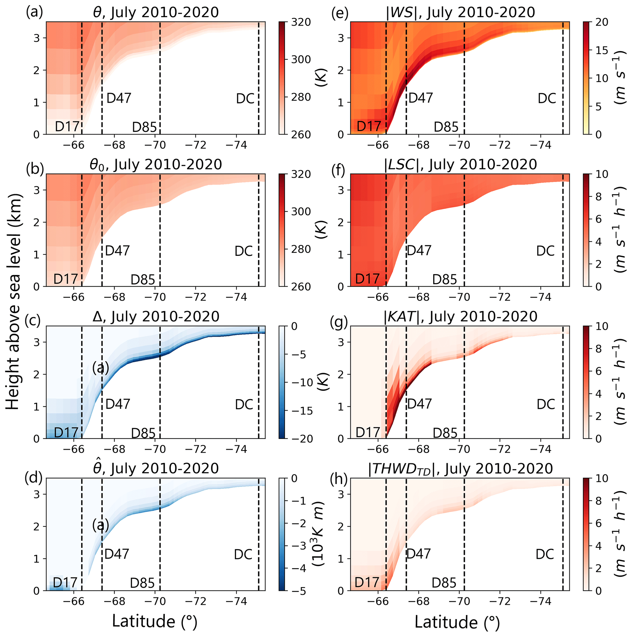
Figure 4Vertical profiles on the transect averaged for the months of July 2010–2020 of (a) potential temperature (θ), (b) background potential temperature (θ0), (c) potential temperature deficit (Δθ), (d) vertically integrated potential temperature deficit (), (e) norm of wind speed (), (f) norm of large-scale acceleration (), (g) norm of katabatic acceleration (), and (h) norm of thermal-wind acceleration ().
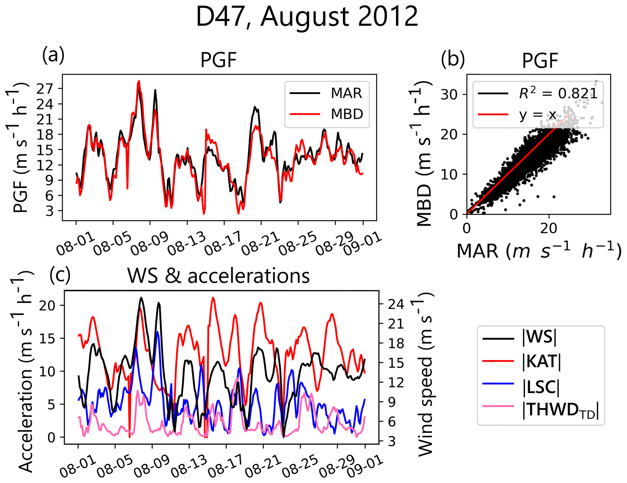
Figure 5Comparison of MAR pressure gradient force (PGF) output with our MBD PGF at D47 at the surface. (a) 3-hourly time series comparison of MAR PGF versus MBD PGF for a winter month (August 2012). (b) Scatter plot of 3-hourly MAR PGF versus MBD PGF for the winter months (June, July, August) of 2010–2020. (c) Wind speed (solid black line) and accelerations used to compute the PGF (katabatic acceleration in red, large-scale acceleration in blue, and thermal-wind acceleration in pink).
The MBD captures well the temporal variations and extrema of the pressure gradient force (Fig. 5). Some of the maxima are underestimated (at D47, our MBD exhibits a mean bias of −1.3 ). This is due to the fact that the background potential temperature profile (θ0) is approximated by a linear slope, which is not always exactly the case, and causes an underestimation of the large-scale acceleration, particularly near the coast (D17), where the vertical structure of air masses is more complex. Quantitatively, the normalized root mean square error (NRMSE, i.e. the root mean square error between MAR PGF and our MBD PGF, normalized by the maximum value minus the minimum value of the time series of MAR PGF at each grid cell) was about 7.5 % for July 2010–2020 at the surface. The coefficient of determination between the July datasets is relatively high everywhere on the transect (R2>0.6), with values ranging from 0.61 at D17 to 0.93 at DC. It indicates a good correlation between our MBD and MAR outputs and shows that the MBD is internally consistent. The approximations described in Sect. 2.2.1 do not introduce significant errors.
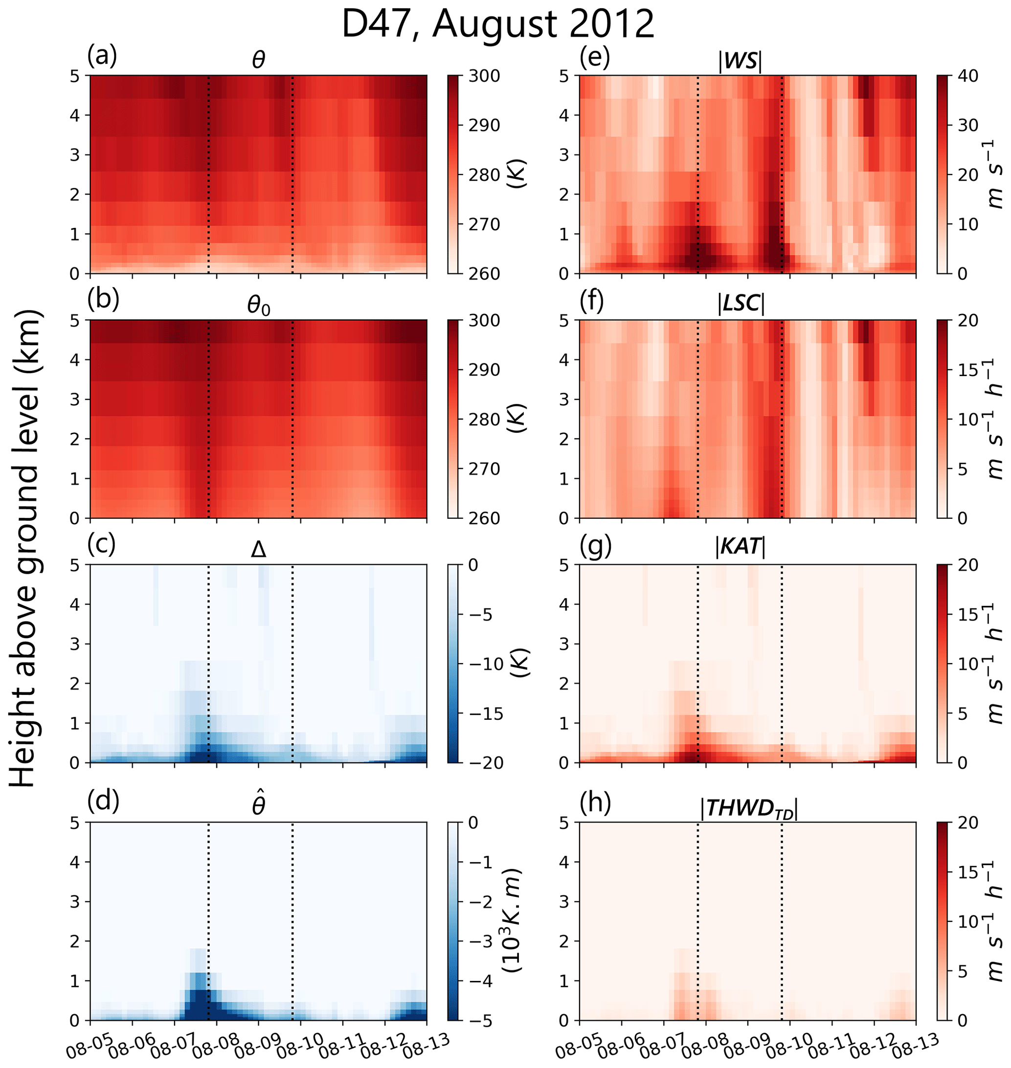
Figure 6Time series of vertical profiles during two high-wind-speed events at D47 on 7 and 9 August 2012 (denoted by vertical dotted lines): (a) potential temperature (θ), (b) background potential temperature (θ0), (c) potential temperature deficit (Δθ), (d) vertically integrated potential temperature deficit (, (e) norm of total wind speed (), (f) norm of large-scale acceleration (), (g) norm of katabatic acceleration (), and (h) norm of thermal-wind acceleration ().
3.3 Evaluation of the momentum budget decomposition (MBD) during a high-wind-speed event
MAR MBD is performed in August 2012 for two successive high-wind-speed events (HWSEs). HWSEs are defined as days for which the total wind speed is greater than the 90th percentile of the 10-year 3-hourly dataset. During the first event on 7 August, the katabatic layer (the air mass cooled down by the surface) starts growing around 00:30 UTC, reaches its maximum around 19:30 UTC (Fig. 6a), and decreases during the next 24 h. This is accompanied by an increase in background potential temperature (up to 288 K; Fig. 6b), which, combined with the low potential temperature at the surface, creates a strong potential temperature inversion ( K; Fig. 6c) and vertically integrated potential temperature deficit (Fig. 6d). This katabatic layer development is characteristic of a katabatic event (Vihma et al., 2011). It is consistent with the computed katabatic acceleration (Fig. 6g), which develops and reaches a maximum on that day, while the large-scale acceleration does not exhibit any significant increase. As a conclusion, the strong wind speed maximum on 7 August is primarily driven by the katabatic acceleration, and we consider it to be a katabatic-driven event.
On the other hand, 2 d later, on 9 August, another peak of wind speed extends much higher in the atmosphere. This time, the temperature deficit at the surface is limited (°; Fig. 6c), and the katabatic acceleration, while present, remains limited. The large-scale acceleration, however, increases progressively, starting on 8 August from 16:30 UTC to its maximum on 9 August at 13:30 UTC (Fig. 6f), just before the wind speed maximum around 19:30 UTC (Fig. 6e). Therefore, this high-wind-speed event is attributed mainly to large-scale forcing.
As a conclusion, our MBD produces logical results in regards to the vertical structure of the atmosphere. It also confirms hints of katabatic events, visible in the development of the katabatic layer in the vertical profile of potential temperature, and provides us with additional information regarding synoptic events, enabling us to clearly identify the main driver of these high-wind-speed events. It also underlines the necessity of studying these events at a 3-hourly timescale in order to be able to capture the variations in the katabatic layer and the large-scale acceleration.
4.1 Quasi-stationary momentum budget and dominant components
The seven terms in the momentum budget – Eqs. (6) and (7) – do not share equal roles in shaping the wind speed intensity or variability. Three of them, katabatic, thermal wind, and large-scale, can be viewed as active terms because they are produced by a forcing, either large-scale or surface pressure gradients. By opposition, turbulence, Coriolis, and advection accelerations can be viewed as passive terms, as they only come into play when the motion has been triggered by an active term.
We evaluated the dominant terms in the surface momentum budget by looking at the average amplitude of each acceleration, computed on 3-hourly outputs for the period 2010–2020 in summer (December–January–February, DJF), winter (June–July–August, JJA), and annual mean, shown in Table 3. The temporal derivative of the wind vector, , is 5 orders of magnitude smaller than the other accelerations. Therefore we can assume a quasi-stationary momentum budget everywhere on the transect, and the total wind speed is directly related to the norm of the sum of the other accelerations through the quasi-geostrophic equilibrium:
with being the geostrophic wind equivalent to each MBD acceleration, i.e. the stationary wind vector that would result from a balance of the acceleration under consideration with the Coriolis acceleration.
Table 3Averaged 2010–2020 summer (DJF), winter (JJA), and annual (Ann) norm of accelerations: katabatic (KAT), large-scale (LSC), thermal-wind (THWDTD), total pressure gradient force (PGF), horizontal advection (ADVH), Coriolis (COR), and turbulent (TURB) accelerations, as well as derivatives with respect to time of the wind speed (|∇tWS|), for the four stations of the transect. Accelerations displaying the highest values for each stations are denoted by a black asterisk. The seasonal values are computed in . Norms are computed with MAR 3-hourly outputs.
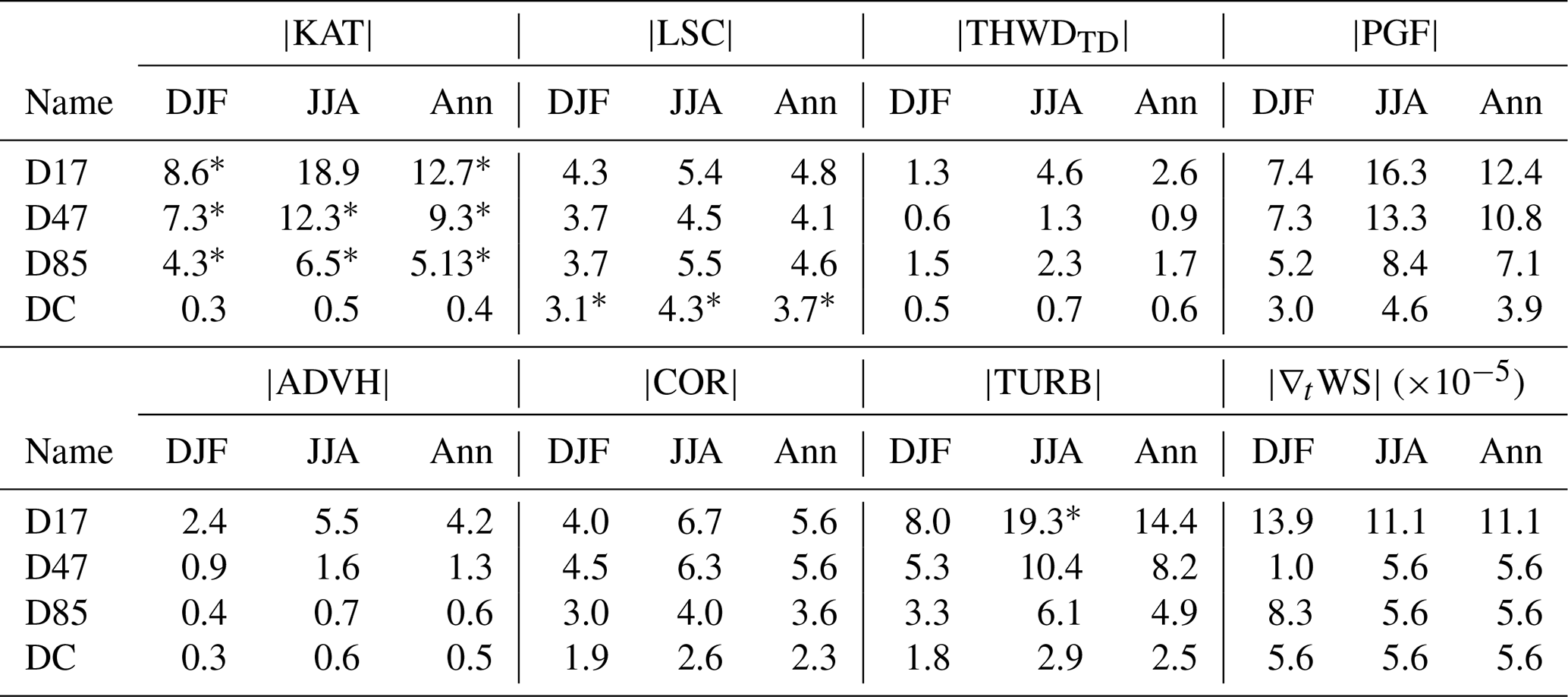
The katabatic, large-scale, and turbulent accelerations are the three dominant terms (Table 3). These three terms alone in Eq. (11) are enough to reproduce the direction and intensity of the near-surface wind (Fig. S7). Horizontal advection and thermal-wind accelerations have lower magnitudes but become significant with regard to the other terms close to the coast (D47 and D17) and over the ocean (Fig. 7).
4.2 Drivers of spatial wind variability
In Antarctica, the wind speed generally increases from the plateau to the coast (Fig. 1). On the transect, mean July 2010–2020 3-hourly MAR wind speeds are ranging from 4.9 to 14.1 m s−1, with a spatial standard deviation of 2.6 m s−1. During summer, mean wind speeds are lower, ranging from 3.6 to 9.1 m s−1 with a spatial standard variation reduced to 1.7 m s−1.
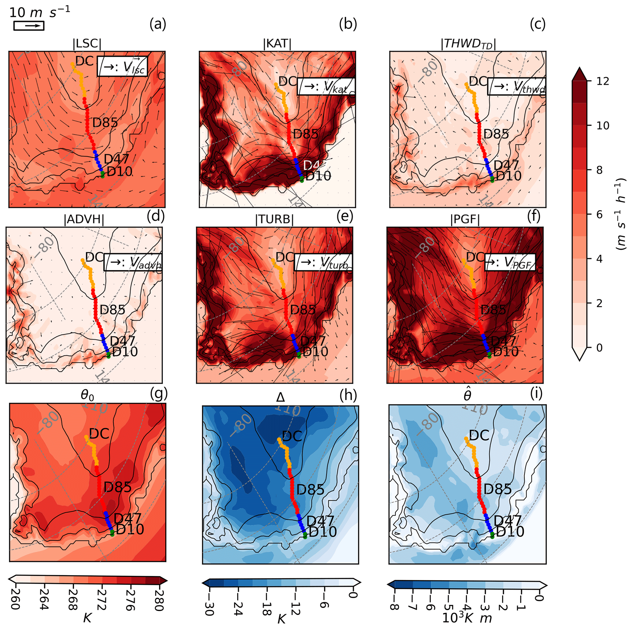
Figure 7Upper and middle panels: mean July 2010–2020 norm of accelerations at surface level (∼ 7 m a.g.l.) computed with 3-hourly MAR outputs: (a) large-scale, (b) katabatic, (c) thermal wind, (d) horizontal advection, (e) turbulence, and (f) pressure gradient force. Superimposed are the equivalent wind vectors. Lower panels: mean July 2010–2020 values of (g) the background temperature θ0, (h) the potential temperature deficit Δθ, and (i) the vertically integrated potential temperature deficit at surface level (∼ 7 m a.g.l.) computed with 3-hourly MAR outputs.
The katabatic acceleration is proportional to the product of the surface slope and the potential temperature deficit (Eq. 3). On the plateau, although the potential temperature deficit Δθ is large (Fig. 7h), the slope is near zero, and the katabatic acceleration is negligible (Fig. 7b). The katabatic acceleration increases strongly in a band of 250 km along the coast, where the surface slope is significant. We refer to this narrow band of strong katabatic acceleration as the active katabatic belt. Here, we want to emphasize that the katabatic acceleration points in the slope direction (see Fig. S8 in the Supplement). As we are in the quasi-geostrophic stationary conditions detailed in Sect. 4.1, we can neglect the first temporal derivative of wind speed. Consequently, the resulting wind speed is the sum of all the equivalent geostrophic wind speeds associated with the five accelerations detailed in Fig. 7a–e. Therefore, we show here in Fig. 7 the direction of the equivalent geostrophic winds (which are rotated by 90° to the left with respect to the acceleration vectors). The same maps with the direction of the acceleration vectors are presented in Fig. S8 of the Supplement.
Wind vectors associated with the katabatic acceleration are therefore always directed in the cross-slope direction. However, note that an increase in the katabatic acceleration does not increase the wind speed purely in the cross-slope direction because of the action of the turbulent acceleration.
There is a secondary, narrower active thermal-wind belt starting ∼ 100 km inland of the coast (Fig. 7c), in which the thermal wind opposes the katabatic acceleration most of the time. This is a consequence of the pressure low created by the displacement of cold air from the inland to the coast. It implies a secondary circulation (thermal wind) in the opposite direction (Parish et al., 1993). Inside this active thermal-wind belt, advection is significant in the valleys (e.g. west of D10 or in the Transantarctic Mountains; Fig. 7d).
The large-scale acceleration (Fig. 7a) is spatially more uniform than the katabatic acceleration (Fig. 7b). The large-scale polar circulation cell is characterized by a high surface pressure on the plateau and lower pressure on the coast. In addition, we find that, on average, the large-scale surface pressure gradient is aligned with the topography, but unlike the katabatic forcing, its value is not proportional to the slope angle. The mean magnitude of the large-scale acceleration is weaker than the katabatic term everywhere on the transect, except at Dome C (Table 3). The magnitude of the large-scale acceleration term varies greatly with a changing synoptic situation. In winter, at D47, for instance, the large-scale acceleration displays a mean value of 5.4 but a value of the 99th percentile (computed with 3-hourly outputs) of about 12.6 m s−1 h−1, which is comparable to the mean value of the katabatic acceleration for that period. The weaker mean intensity is due to the changing location of synoptic perturbations.
The turbulent acceleration mostly encompasses drag and vertical advection (supposed negligible by van den Broeke and van Lipzig, 2003). The drag is proportional and in the opposing direction to the wind vector (Fig. 7e).
To sum up, the mean acceleration of the wind on the slope of the plateau is dominated by the katabatic forcing, but the large-scale forcing also plays a role, as it has the same spatial pattern and the same sign, albeit with a smaller amplitude in the active katabatic belt. These two forcings are opposed by turbulence and by thermal wind very close to the coast, causing the wind speed maximum to be slightly more upslope than the slope would dictate alone.
4.3 Drivers of seasonal wind variability on the transect
The wind speed displays a seasonal cycle that peaks in late winter (August to September) and is especially pronounced in the low-elevation and coastal areas. In Fig. 8, we compute the annual cycle of the total wind speed (average of 3-hourly time steps for 2010–2020) and of wind speed equivalent to large-scale (VLSC), thermal-wind (), katabatic (VKAT), and turbulent accelerations (VTURB). Below 1500 m, the seasonal amplitude in wind speed between summer and winter ( equals 5.6 m s−1 at D17 and 3.8 m s−1 at D47) is larger than the July standard deviation of 3-hourly July wind speed (highest variability during winter months) computed over the 10-year dataset ( equals 4.1 m s−1 at D17 and 3.4 m s−1 at D47). In higher-elevation and interior zones, the seasonal cycle is much weaker, and the 10-year standard deviation of July 3-hourly wind speed exceeds .
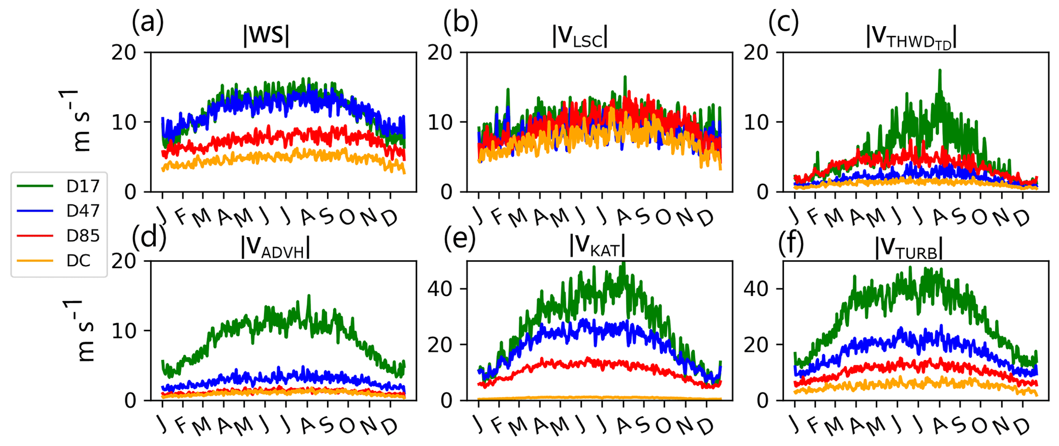
Figure 8Seasonal cycle of 3-hourly near-surface winds averaged over 10 years for (a) total wind speed, (b) wind speed equivalent to large-scale acceleration, (c) wind speed equivalent to thermal wind, (d) wind speed equivalent to advection, (e) wind speed equivalent to horizontal katabatic acceleration, and (f) wind speed equivalent to turbulent acceleration. Note that the y axis is different between panels (a)–(d) (, , , ) and panels (e)–(f) (, ).
Because of the strong seasonal cycle of the temperature deficit, as expected, a similar behaviour for katabatic and thermal winds (which are directly related to the surface inversion) is found. Katabatic winds have a strong seasonal cycle (Fig. 8d) which peaks in August and is increasingly stronger from inland to the coast. The strongest seasonal amplitude is found at D17 ( is 25 m s−1). Note that the seasonal amplitude of katabatic winds is significantly stronger than that of the total wind speed because it is damped by turbulence, which also displays a strong seasonal cycle ( is 22 m s−1). Thermal wind also depends on the inversion layer but is concentrated near the coastline (Fig. 7c) and shows a strong seasonality for D17 exclusively ( is 3.6 m s−1).
Surprisingly, the thermal wind is stronger at D85 than at D47, closer to the coast. This is due to the small valley shape around D85 (Fig. 1b) that enables piling up of cold air coming from the plateau (Fig. 4d), while D47 is located in the middle of a steep slope. Unlike surface-related momentum contributions, large-scale winds exhibit a weak seasonal cycle, identical for all stations, with ranging from 1.4 for D47 to 2.7 m s−1 for D85. Therefore the large-scale contribution is unlikely to explain either the seasonal variability in the total wind speed or the spatial differences in the seasonal cycle along the transect. Advection is computed as the scalar product of the wind vector and its horizontal gradient. It is significant only at D17 where wind speed exhibits a larger spatial variability.
From these analyses and from the Supplement analyses (Fig. S12), we conclude that the seasonal variability in wind speed is mainly produced by the seasonal cycle of katabatic acceleration, which is proportional to the surface inversion strength. The large-scale forcing only plays a minor role in the seasonal cycle of near-surface wind.
4.4 Drivers of 3-hourly winter variability
In this section, we investigate the drivers of near-surface wind variability at the synoptic scale. We analyse the high-temporal-resolution wind speed output (3-hourly) for the months of July 2010–2020, when wind speeds are particularly high (seasonal maximum) and the diurnal cycle is very weak (polar night). We use the correlation coefficients between the different accelerations and the total wind speed to identify the dominant drivers of wind speed variability (Fig. 9).
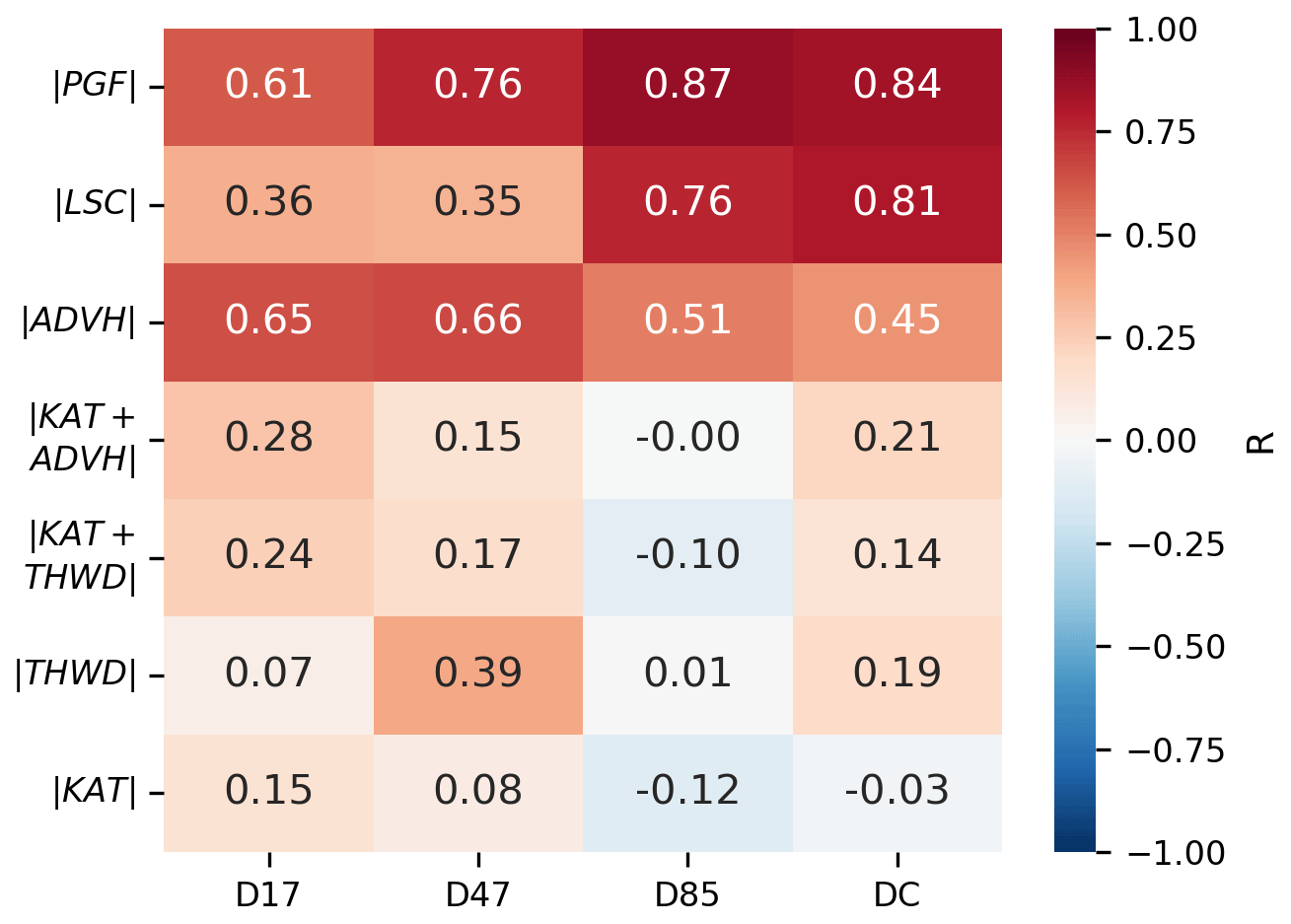
Figure 9Correlation coefficient (R) between the 3-hourly total wind speed and the different accelerations in July 2010–2020.
Table 4July 2010–2020 statistics for katabatic (KAT), large-scale (LSC), thermal-wind (THWDTD), surface process (KAT+THWDTD), and total pressure gradient force (PGF) accelerations for the four stations on the transect. The averaged value (Avg.) and standard deviation (σ) are computed in . R is the correlation coefficient with the total wind speed. All metrics are computed with MAR 3-hourly outputs for July 2010–2020.
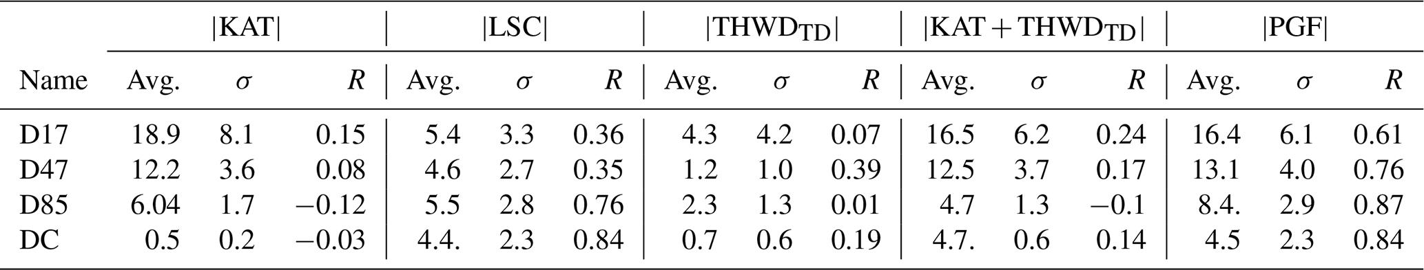
In the regions where the katabatic acceleration is small (D85 and DC; see Table 4 or Fig. 9), as expected, the correlation coefficient between the large-scale acceleration and the total wind speed is very high (R>0.75). Closer to the coast, this correlation coefficient decreases, reaching ∼0.35 for both D17 and D47. There, although the katabatic acceleration becomes stronger (greater than 12 on average in the winter, more than twice the value of the mean large-scale acceleration; Table 4), the acceleration remains poorly correlated with the total wind speed (R respectively equals 0.15 and 0.08 for D17 and D47). At these specific locations, it seems that none of the decomposed accelerations singularly dominate the 3-hourly wind speed variability.
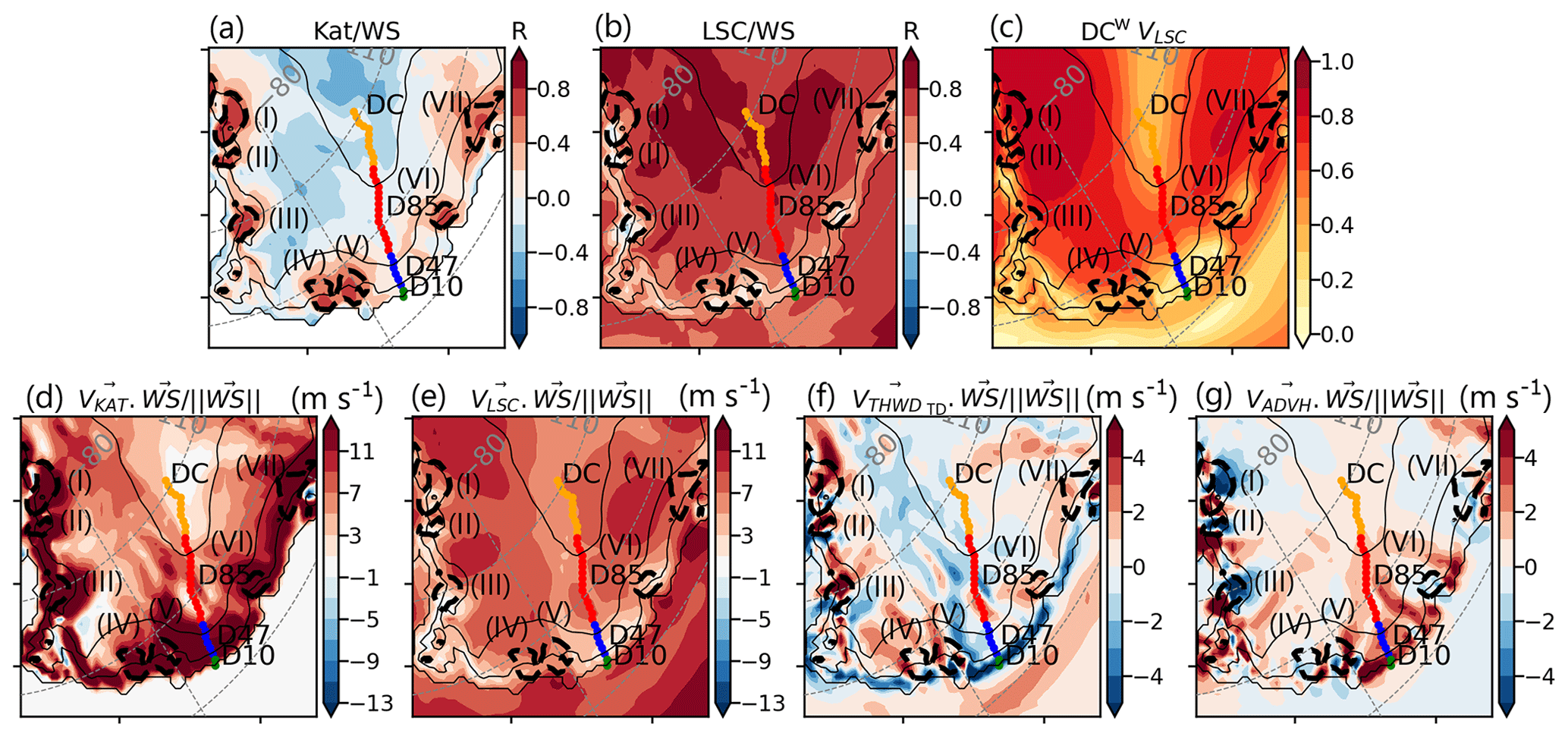
Figure 10(a) Average July 2010–2020 correlation coefficient of 3-hourly katabatic acceleration and wind speed, (b) average July 2010–2020 correlation coefficient of 3-hourly large-scale acceleration, and (c) wind speed directional constancy of 3-hourly large-scale wind speed. (d, e, f) Mean of 3-hourly July 2010–2020 scalar product normalized by the norm of wind speed of (d) 3-hourly katabatic wind speed and total wind speed, (e) 3-hourly large-scale and total wind speed, (f) 3-hourly thermal wind and total wind speed, and (g) 3-hourly advection and total wind speed. For the seven panels, the dotted black line corresponds to the line for which the correlation coefficient of katabatic acceleration and total wind speed reaches 0.5. Seven zones of higher correlations are indicated: (I), (II), (III), (IV), (V), (VI), and (VII).
Before explaining these results on the transect, we want to test how well our transect represents the coastal region of Adélie Land. To this aim, we analyse the correlation coefficient between the katabatic acceleration and the total wind speed, not only on the transect but rather on a surrounding region of 1800 km × 1550 km centred on Adélie Land (Fig. 10a). In the active katabatic belt, some regions show a higher correlation (R>0.5) between the katabatic acceleration and the total wind speed. Our transect is located right in the middle between two of these regions, meaning that it is not necessarily representative of the whole region.
A first explanation to the low correlation between the katabatic acceleration and the total wind speed could be that, close to the coast, the thermal wind opposes the katabatic acceleration. Thus, the sum of katabatic and thermal-wind accelerations (, in other words, surface processes) displays a better correlation with the total wind speed (R=0.24 at D17 and R=0.17 at D47) than the katabatic acceleration alone (, R=0.15 at D17 and R=0.08 at D47; Table 4, Fig. 9). Considering surface processes together prevents us from overestimating the impact of the katabatic acceleration, especially in cases where both thermal-wind and katabatic acceleration are large but of opposite direction.
In order to test this hypothesis on the whole region, we compute the scalar product of mean July 2010–2020 thermal wind with the wind direction. It enables us to assess whether thermal wind actively opposes the wind (negative values) or acts in a direction that increases it (positive values; Fig. 10f).
We observe that out of the seven zones of higher correlation between the katabatic acceleration and the total wind speed (R>0.5; Fig. 10a), five of them correspond to locations where the action of thermal wind is positive (Fig. 10f II, III, V, VI, VII). In the other ones (I, IV), the scalar product of total wind speed and thermal wind is close to zero (IV), indicating that the thermal wind has no effect on the total wind speed or includes some area of negative values (I). Note that some area of positive action of thermal-wind and strong katabatic accelerations (e.g. west and south of I) do not create the conditions for a strong correlation of the katabatic acceleration and the total wind speed. Therefore, the acceleration provided by thermal wind is not sufficient to fully explain the locations of the highest values of the correlation between the katabatic acceleration and the total wind speed. Similarly, the effect of advection cannot fully explain strong correlations between katabatic acceleration and total wind speed. Areas of strong correlation correspond either to locations of strong negative and positive advection contributions (I, II, III) or to a weak advection contribution (IV, V, VI, VII).
While the katabatic acceleration is always directed downslope, the large-scale wind speed displays a much more variable direction, indicated by low values of directional constancy (DCwVLSC) (see Fig. 10c). DCw is computed as follows:
On the plateau, DCw is close to zero, which is typical of a wind with no preferred direction. In the valleys around and in the higher-elevation zone, winds tend to blow in a preferred downslope direction and DCw is closer to 1. However, from D47 to the coast, DCw falls back to zero. That part of the segment is located on a ridge. As a result, the topographic steering of surface pressure gradient is less important than in the valleys. In locations with small DCw (i.e. on ridges and plateaus), the large-scale pressure gradient sometimes opposes the katabatic acceleration, leading to decreased correlations of the katabatic acceleration with total wind speed.
Figure 11Correlations for July 2010–2020, 3-hourly, between the large-scale acceleration and the total wind speed at (a) D17 (coast), (b) D47, (c) D85, and (d) DC (plateau). The colorbar indicates the absolute value of the angle between the katabatic and the large-scale acceleration. Around 0°, LSC and KAT are aligned; around 180°, they are of opposite direction.
The angle between the large-scale acceleration and the topography seems to have a major impact on the wind speed intensity. This is confirmed by Fig. 11, where we find a clear partition of the influence of the angle: the wind speed is higher when the large-scale acceleration is aligned with the topography (angle 0°, blue in Fig. 11) and weaker when the large-scale acceleration opposes the katabatic acceleration (angle 180°, red dots in Fig. 11). In locations where the large-scale direction is highly variable (e.g. between D10 and D47, close to the coast), the angle between katabatic and large-scale acceleration displays both positive and negative values. In this situation, there is not a single driver of the wind speed intensity but rather a competition between katabatic acceleration (mainly in winter and at night) and large-scale forcing which is particularly effective when it is aligned with the katabatic acceleration. Therefore, it is essential to compute the momentum budget decomposition in order to identify the drivers of wind speed variability.
To sum up, the dominant drivers of synoptic-scale variability depend on the location. On the plateau, the large-scale forcing logically dominates the variability. In the active katabatic belt, the katabatic acceleration has the strongest amplitude and variance (Table 4). However, a strong katabatic forcing is not always causing high wind speed because the large-scale acceleration can counteract the katabatic acceleration, if it is oriented upslope. Thus, the angle between the large-scale acceleration and the surface slope is a key factor in explaining strong wind speed events in coastal Antarctica: the highest-wind-speed events happen when the katabatic and large-scale forcing are aligned (Fig. 11), although each acceleration, when acting alone, can also cause strong wind speed (Fig. 6). On the coast, the pile-up of cold air at sea level counteracts the katabatic forcing, which explains why the strongest wind speeds are not found right on the coast (Fig. 7). There, all of the terms of the momentum budget are important, and there is not a dominant forcing term. We demonstrated that, although the katabatic term is the dominant contributor to the mean wind speed, spatially and seasonally, at the event scale, accelerations are more complex, and wind events cannot systematically be interpreted as katabatic.
In this study, we obtained a comprehensive understanding of the drivers of East Antarctic near-surface winds by combining directional consistency and momentum budget decomposition analyses. As different accelerations can cancel each other when in opposing directions, the consistent directional behaviour of the wind serves as a valuable complementary tool to the MBD for examining the drivers of near-surface winds in the active katabatic region. It reveals locations where correlation of the katabatic acceleration with the wind speed is weak due to the variable large-scale wind direction. However, we show that relying solely on directional constancy does not provide a reliable diagnosis of near-surface wind drivers because large-scale winds exhibit areas of significant directional consistency in regions where katabatic acceleration is low and does not correlate with wind speed, in line with Parish and Cassano (2003).
Previous work using the MBD had focused on monthly averages (van den Broeke and van Lipzig, 2003; Bintanja et al., 2014). However, to understand the drivers of high-wind-speed events, it is necessary to study winds at a sub-daily resolution. Here we have demonstrated that variations in the temperature deficit strength or in large-scale pressure gradient occur within a day (e.g. Fig. 6). Therefore, to highlight the influence of synoptic events on the nature of near-surface winds in the active katabatic belt, we have selected a 3-hourly time step. In this pursuit, we have adapted the method for extrapolating the free-atmosphere vertical potential temperature profile θ0 developed by van den Broeke and van Lipzig (2003) for monthly outputs. However, the linearization of the vertical potential temperature profile is challenging with 3-hourly outputs. Most of the profiles featuring a large normalized root mean square error (NRMSE) between the native MAR PGF and our MBD PGF, i.e. greater than the 90 % percentile (which corresponds approximatively to a NRMSE greater than 10 %; Fig. S10) do not feature any abrupt increase in the vertical derivative of potential temperature at the top of the inversion layer, leading to an underestimation of the MBD PGF. Some other profiles display intrusions of air-masses (characterized by a non-strictly monotonous profile of potential temperature) or a secondary linear section with a different slope under 500 hPa. Examples of these types of profiles are shown in Fig. S11. From the comparison between PGFMAR and our PGFMBD, our MBD works better in the interior than close to the coast, where these types of profiles are more likely to be found, probably due to the vicinity of the ocean. Overall, on our transect, there is a satisfactory low number of profiles exhibiting large NRMSE. Increasing the temporal resolution of our dataset would be even more challenging. The vertical profiles of potential temperature would be even less smooth and hard to interpolate. Furthermore, the stationary approximation has been made at a 3-hourly timescale, which is generally valid (Sect. 4.1) but might not be accurate at a finer resolution.
Finally, it is crucial to have a good depiction of the vertical structure of the atmosphere, inside and above the boundary layer, to study the drivers of near-surface winds. Our regional atmospheric model has been evaluated at 2 m a.g.l. and performs well at that height. However, its ability to accurately represent vertical atmospheric profiles has not been assessed due to limited observations, only available at DC where there is no katabatic acceleration and DDU where the performance of MAR is limited. In the future, it would be valuable to have available radiosoundings in a katabatic-active region to conduct an observational study about the drivers of near-surface winds and to evaluate more accurately our model.
To understand the drivers of near-surface winds in Antarctica, we have separated the contributions to wind speed of surface-based and large-scale pressure gradients using the momentum budget decomposition. We focused on a well-instrumented transect running through Adélie Land (east Antarctica), from the plateau to the coast. We demonstrated that seasonal and spatial variabilities in near-surface winds in Adélie Land are both dominated by surface processes, notably by katabatic winds. At a 3-hourly timescale, however, on our study transect, identifying the main driver of the wind becomes more challenging. Large-scale pressure acceleration correlates well to the total wind speed from the plateau to ∼ 250 km from the coast in locations where the katabatic acceleration is weak to null. Then, in the active katabatic and thermal-wind belt, below 2000 m above sea level, surface processes come into play and decrease the correlation of large-scale acceleration with the total wind speed. Due to the highly varying angle between large-scale and katabatic accelerations, close to the coast, the two are often in competition. Thus, correlation coefficients of large-scale and katabatic processes with total wind speed remain low, weaker than respectively 0.4 and 0.2. In that region of the transect, at a 3-hourly timescale, even though the katabatic acceleration reaches average values greater than 40 , it cannot be considered the unique driver of near-surface wind variability. The variability in the near-surface winds in the lowest section of the transect is the result of variability in the intensity of both large-scale and katabatic processes as well as variability in the angle between these two accelerations.
Our momentum budget decomposition study unveils deeper insights into the relationship between the magnitude of different accelerations and their correlation with the total wind speed. It underscores the limitation of assessing the synoptic or katabatic nature of near-surface winds solely by studying the individual magnitudes of accelerations on a 3-hourly timescale. In locations where there is not a single driver of temporal variability, high-wind-speed events can be synoptic-driven, surface-driven, or a combination of both when they act in the same direction.
All data and scripts developed in this study to compute each momentum budget acceleration for July 2010 are available at https://doi.org/10.5281/zenodo.8315142 (Davrinche et al., 2023).
The supplement related to this article is available online at: https://doi.org/10.5194/tc-18-2239-2024-supplement.
CD, CeA, and AO designed the study and contributed to the output and observation analyses. CeA, ChA, and CK set up the MAR model for Antarctica with several adaptations. CeA performed model simulations and the MAR PGF diagnostic. CD performed the momentum budget decomposition, assembled observational data, post-processed the data, did the bulk of the analysis, and made all the figures. CD wrote the first draft, with input from CeA and AO. All authors contributed to discussions in writing this paper.
The contact author has declared that none of the authors has any competing interests.
Publisher’s note: Copernicus Publications remains neutral with regard to jurisdictional claims made in the text, published maps, institutional affiliations, or any other geographical representation in this paper. While Copernicus Publications makes every effort to include appropriate place names, the final responsibility lies with the authors.
The authors appreciate the support of the University of Wisconsin–Madison Automatic Weather Station Program for the dataset, data display, and information (NSF grant number 1924730). We acknowledge using data from the CALVA project and CENECLAM and GLACIOCLIM observatories. This work is part of the Katabatic project, AWACA project, and the POLARiso project. The MAR simulations were performed thanks to access granted to the HPC resources of IDRIS under the allocation 2022-AD010114000 made by GENCI. We acknowledge the work of Xavier Fettweis (Université de Liège) in developing and maintaining the MAR model.
This research has been funded by the Agence Nationale de la Recherche JCJC Katabatic project (grant no. ANR19-CE01-0020-01) awarded to Anaïs Orsi and by NSERC Discovery (grant no. DGERC-2021-00213). This work is also part of the AWACA project that has received funding from the European Research Council (ERC) under the European Union's Horizon 2020 research and innovation programme (grant agreement no. 951596) and part of the POLARiso project that has received funding from the European Union's Horizon 2020 research and innovation programme under the Marie Skłodowska-Curie action (grant agreement no. 8410).
This paper was edited by Michiel van den Broeke and reviewed by two anonymous referees.
Agosta, C., Amory, C., Kittel, C., Orsi, A., Favier, V., Gallée, H., van den Broeke, M. R., Lenaerts, J. T. M., van Wessem, J. M., van de Berg, W. J., and Fettweis, X.: Estimation of the Antarctic surface mass balance using the regional climate model MAR (1979–2015) and identification of dominant processes, The Cryosphere, 13, 281–296, https://doi.org/10.5194/tc-13-281-2019, 2019. a, b, c
Amory, C., Trouvilliez, A., Gallée, H., Favier, V., Naaim-Bouvet, F., Genthon, C., Agosta, C., Piard, L., and Bellot, H.: Comparison between observed and simulated aeolian snow mass fluxes in Adélie Land, East Antarctica, The Cryosphere, 9, 1373–1383, https://doi.org/10.5194/tc-9-1373-2015, 2015. a
Amory, C., Gallée, H., Naaim-Bouvet, F., Favier, V., Vignon, E., Picard, G., Trouvilliez, A., Piard, L., Genthon, C., and Bellot, H.: Seasonal variations in drag coefficient over a sastrugi-covered snowfield in coastal East Antarctica, Bound.-Lay. Meteorol., 164, 107–133, https://doi.org/10.1007/s10546-017-0242-5, 2017. a, b
Amory, C., Kittel, C., Le Toumelin, L., Agosta, C., Delhasse, A., Favier, V., and Fettweis, X.: Performance of MAR (v3.11) in simulating the drifting-snow climate and surface mass balance of Adélie Land, East Antarctica, Geosci. Model Dev., 14, 3487–3510, https://doi.org/10.5194/gmd-14-3487-2021, 2021. a, b
AWS: Data and Imagery – AMRC/AWS, https://amrc.ssec.wisc.edu/data/ (last access: 24 April 2024), 2010. a
Ball, F.: The Theory of Strong Katabatic Winds, Aust. J. Phys., 9, 373–386, https://doi.org/10.1071/PH560373, 1956. a
Bintanja, R.: The contribution of snowdrift sublimation to the surface mass balance of Antarctica, Annals of Glaciology, 27, 251–259, https://doi.org/10.3189/1998AoG27-1-251-259, 1998. a
Bintanja, R., Severijns, C., Haarsma, R., and Hazeleger, W.: The future of Antarctica's surface winds simulated by a high-resolution global climate model: 2. Drivers of 21st century changes, J. Geophys. Res.-Atmos., 119, 7160–7178, https://doi.org/10.1002/2013JD020848, 2014. a, b
Bracegirdle, T. J., Connolley, W. M., and Turner, J.: Antarctic climate change over the twenty first century, J. Geophys. Res., 113, D03103, https://doi.org/10.1029/2007JD008933, 2008. a
Brun, E., David, P., Sudul, M., and Brunot, G.: A numerical model to simulate snow-cover stratigraphy for operational avalanche forecasting, J. Glaciol., 38, 13–22, https://doi.org/10.3189/S0022143000009552, 1992. a
Davrinche, C., A., Anaïs, O., Christoph, K., and Charles, A.: Understanding the drivers of winter surface winds intensity in Adelie land, Zenodo [data set and code], https://doi.org/10.5281/zenodo.8315142, 2023. a
Fretwell, P., Pritchard, H. D., Vaughan, D. G., Bamber, J. L., Barrand, N. E., Bell, R., Bianchi, C., Bingham, R. G., Blankenship, D. D., Casassa, G., Catania, G., Callens, D., Conway, H., Cook, A. J., Corr, H. F. J., Damaske, D., Damm, V., Ferraccioli, F., Forsberg, R., Fujita, S., Gim, Y., Gogineni, P., Griggs, J. A., Hindmarsh, R. C. A., Holmlund, P., Holt, J. W., Jacobel, R. W., Jenkins, A., Jokat, W., Jordan, T., King, E. C., Kohler, J., Krabill, W., Riger-Kusk, M., Langley, K. A., Leitchenkov, G., Leuschen, C., Luyendyk, B. P., Matsuoka, K., Mouginot, J., Nitsche, F. O., Nogi, Y., Nost, O. A., Popov, S. V., Rignot, E., Rippin, D. M., Rivera, A., Roberts, J., Ross, N., Siegert, M. J., Smith, A. M., Steinhage, D., Studinger, M., Sun, B., Tinto, B. K., Welch, B. C., Wilson, D., Young, D. A., Xiangbin, C., and Zirizzotti, A.: Bedmap2: improved ice bed, surface and thickness datasets for Antarctica, The Cryosphere, 7, 375–393, https://doi.org/10.5194/tc-7-375-2013, 2013. a
Gallée, H. and Pettré, P.: Dynamical Constraints on Katabatic Wind Cessation in Adélie Land, Antarctica, J. Atmos. Sci., 55, 1755–1770, https://doi.org/10.1175/1520-0469(1998)055<1755:DCOKWC>2.0.CO;2, 1998. a, b
Gallée, H. and Schayes, G.: Development of a three-dimensional meso-γ primitive equation model: katabatic winds simulation in the area of Terra Nova Bay, Antarctica, Mon. Weather Rev., 122, 671–685, https://doi.org/10.1175/1520-0493(1994)122<0671:DOATDM>2.0.CO;2, 1994. a
Genthon, C., Town, M. S., Six, D., Favier, V., Argentini, S., and Pellegrini, A.: Meteorological atmospheric boundary layer measurements and ECMWF analyses during summer at Dome C, Antarctica, J. Geophys. Res.-Atmos., 115, D05104, https://doi.org/10.1029/2009JD012741, 2010. a
Genthon, C., Veron, D., Vignon, E., Six, D., Dufresne, J. L., Madeleine, J.-B., Sultan, E., and Forget, F.: Ten years of wind speed observation on a 45-m tower at Dome C, East Antarctic plateau, PANGAEA [data set], https://doi.org/10.1594/PANGAEA.932513, 2021. a
Gerber, F., Sharma, V., and Lehning, M.: CRYOWRF-a validation and the effect of blowing snow on the Antarctic SMB, Authorea Preprints, 2023.. a
Gorter, W., van Angelen, J. H., Lenaerts, J. T. M., and van den Broeke, M. R.: Present and future near-surface wind climate of Greenland from high resolution regional climate modelling, Clim. Dynam., 42, 1595–1611, https://doi.org/10.1007/s00382-013-1861-2, 2014. a
Grazioli, J., Madeleine, J.-B., Gallée, H., Forbes, R. M., Genthon, C., Krinner, G., and Berne, A.: Katabatic winds diminish precipitation contribution to the Antarctic ice mass balance, P. Natl. Acad. Sci. USA, 114, 10858–10863, https://doi.org/10.1073/pnas.1707633114, 2017. a
Hazel, J. E. and Stewart, A. L.: Are the Near-Antarctic Easterly Winds Weakening in Response to Enhancement of the Southern Annular Mode?, J. Clim., 32, 1895–1918, https://doi.org/10.1175/JCLI-D-18-0402.1, 2019. a
Hersbach, H., Bell, B., Berrisford, P., Hirahara, S., Horányi, A., Muñoz-Sabater, J., Nicolas, J., Peubey, C., Radu, R., Schepers, D., and others: The ERA5 global reanalysis, Q. J. Roy. Meteorol. Soc., 146, 1999–2049, https://doi.org/10.1002/qj.3803, 2020. a
Hillebrandt, W. and Kupka, F.: An Introduction to Turbulence, in: Interdisciplinary Aspects of Turbulence, edited by: Hillebrandt, W. and Kupka, F., Lecture Notes in Physics, Springer, Berlin, Heidelberg, 1–20, ISBN 9783540789611, https://doi.org/10.1007/978-3-540-78961-1_1, 2009. a
Hoffmann, L. and Spang, R.: An assessment of tropopause characteristics of the ERA5 and ERA-Interim meteorological reanalyses, Atmos. Chem. Phys., 22, 4019–4046, https://doi.org/10.5194/acp-22-4019-2022, 2022. a
Jullien, N., Vignon, E., Sprenger, M., Aemisegger, F., and Berne, A.: Synoptic conditions and atmospheric moisture pathways associated with virga and precipitation over coastal Adélie Land in Antarctica, The Cryosphere, 14, 1685–1702, https://doi.org/10.5194/tc-14-1685-2020, 2020. a
Kittel, C., Amory, C., Agosta, C., Jourdain, N. C., Hofer, S., Delhasse, A., Doutreloup, S., Huot, P.-V., Lang, C., Fichefet, T., and Fettweis, X.: Diverging future surface mass balance between the Antarctic ice shelves and grounded ice sheet, The Cryosphere, 15, 1215–1236, https://doi.org/10.5194/tc-15-1215-2021, 2021. a, b, c
Lenaerts, J. T. M., Van Den Broeke, M. R., Van De Berg, W. J., Van Meijgaard, E., and Kuipers Munneke, P.: A new, high-resolution surface mass balance map of Antarctica (1979–2010) based on regional atmospheric climate modeling: SMB ANTARCTICA, Geophys. Res. Lett., 39, L04501, https://doi.org/10.1029/2011GL050713, 2012. a
Mahrt, L.: Momentum balance of gravity flows, J. Atmos. Sci., 39, 2701–2711, 1982. a
Mottram, C., Kellett, D., Barresi, T., Zwingmann, H., Friend, M., Todd, A., and Percival, J.: Syncing fault rock clocks: Direct comparison of U-Pb carbonate and K-Ar illite fault dating methods, Geology, 48, 1179–1183, https://doi.org/10.1130/G47778.1, 2020. a
Neme, J., England, M. H., and McC. Hogg, A.: Projected Changes of Surface Winds Over the Antarctic Continental Margin, Geophys. Res. Lett., 49, e2022GL098820, https://doi.org/10.1029/2022GL098820, 2022. a
Parish, T., Pettré, P., and Wendler, G.: The influence of large-scale forcing on the katabatic wind regime at Adélie Land, Antarctica, Meteorol. Atmos. Phys., 51, 165–176, 1993. a
Parish, T. R. and Bromwich, D. H.: A Case Study of Antarctic Katabatic Wind Interaction with Large-Scale Forcing, Mon. Weather Rev., 126, 199–209, https://doi.org/10.1175/1520-0493(1998)126<0199:ACSOAK>2.0.CO;2, 1998. a
Parish, T. R. and Cassano, J. J.: Forcing of the Wintertime Antarctic Boundary Layer Winds from the NCEP–NCAR Global Reanalysis, J. Appl. Meteorol., 40, 810–821, https://doi.org/10.1175/1520-0450(2001)040<0810:FOTWAB>2.0.CO;2, 2001. a
Parish, T. R. and Cassano, J. J.: The role of katabatic winds on the Antarctic surface wind regime, Mon. Weather Rev., 131, 317–333, 2003. a, b, c
Renfrew, I. A. and Anderson, P. S.: The surface climatology of an ordinary katabatic wind regime in Coats Land, Antarctica, Tellus A, 54, 463–484, 2002. a
Sanz Rodrigo, J., Buchlin, J.-M., Van Beeck, J., Lenaerts, J. T. M., and Van Den Broeke, M. R.: Evaluation of the antarctic surface wind climate from ERA reanalyses and RACMO2/ANT simulations based on automatic weather stations, Clim. Dynam., 40, 353–376, https://doi.org/10.1007/s00382-012-1396-y, 2013. a
van den Broeke, M., van Lipzig, N., and van Meijgaard, E.: Momentum budget of the East Antarctic atmospheric boundary layer: Results of a regional climate model, J. Atmos. Sci., 59, 3117–3129, 2002. a, b, c
van den Broeke, M. R. and van Lipzig, N. P. M.: Factors Controlling the Near-Surface Wind Field in Antarctica, Mon.Weather Rev., 131, 733–743, https://doi.org/10.1175/1520-0493(2003)131<0733:FCTNSW>2.0.CO;2, 2003. a, b, c, d, e, f, g
Vignon, É., Traullé, O., and Berne, A.: On the fine vertical structure of the low troposphere over the coastal margins of East Antarctica, Atmos. Chem. Phys., 19, 4659–4683, https://doi.org/10.5194/acp-19-4659-2019, 2019. a
Vihma, T., Tuovinen, E., and Savijärvi, H.: Interaction of katabatic winds and near-surface temperatures in the Antarctic: KATABATIC WINDS IN THE ANTARCTIC, J. Geophys. Res.-Atmos., 116, D21119, https://doi.org/10.1029/2010JD014917, 2011. a, b
Vionnet, V., Brun, E., Morin, S., Boone, A., Faroux, S., Le Moigne, P., Martin, E., and Willemet, J.-M.: The detailed snowpack scheme Crocus and its implementation in SURFEX v7.2, Geosci. Model Dev., 5, 773–791, https://doi.org/10.5194/gmd-5-773-2012, 2012. a
Wendler, G.: Strong gravity flow observed along the slope of Eastern Antarctica: A contribution to I.A.G.O., Meteorol. Atmos. Phys., 43, 127–135, https://doi.org/10.1007/BF01028115, 1990. a
Yasunari, T. and Kodama, S.: Intraseasonal variability of katabatic wind over east Antarctica and planetary flow regime in the southern hemisphere, J. Geophys. Res., 98, 13063, https://doi.org/10.1029/92JD02084, 1993. a