Surface heat fluxes at coarse blocky Murtèl rock glacier (Engadine, eastern Swiss Alps)

We estimate the surface energy balance (SEB) of the Murtèl rock glacier, a seasonally snow-covered permafrost landform with a ventilated coarse blocky active layer (AL) located in the eastern Swiss Alps. We focus on the parameterisation of the turbulent heat fluxes. Seasonally contrasting atmospheric conditions occur in the Murtèl cirque, with downslope katabatic jets in winter and a strongly unstable atmosphere over the heated blocky surface in summer. We use a novel comprehensive sensor array both above the ground surface and in the coarse blocky AL to track the rapid coupling by convective heat and moisture fluxes between the atmosphere, the snow cover, and the AL for the time period September 2020–September 2022. The in situ sensor array includes a sonic anemometer for eddy-covariance flux above-ground and sub-surface long-wave radiation measurements in a natural cavity between the AL blocks. During the thaw seasons, the measurements suggest an efficient (∼ 90 %) export of the available net radiation by sensible and latent turbulent fluxes, thereby strongly limiting the heat available for melting ground ice. Turbulent export of heat and moisture drawn from the permeable AL contributes to the well-known insulating effect of the coarse blocky AL and partly explains the climate resiliency of rock glaciers. This self-cooling capacity is counteracted by an early snow melt-out date, exposing the low-albedo blocky surface to the intense June–July insolation and causing reduced evaporative cooling due to exacerbated moisture scarcity in the near-surface AL during dry spells. With climate change, earlier snowmelt and increased frequency, duration, and intensity of heat waves and droughts are projected. Regarding the parameterisation of the turbulent fluxes, we estimated the year-round turbulent fluxes using a modified Louis (1979) scheme. The monthly SEB is closed within 20 W m⁻² except during the snowmelt months and under katabatic drainage winds in winter. Detected sensible turbulent fluxes from nocturnal ventilation processes, although a potentially important ground cooling mechanism, are within our 20 W m⁻² uncertainty because nighttime wind speeds are low. Wintertime katabatic wind speeds needed to be scaled to close the SEB, which hints at the limits of parameterisations based on the Monin–Obukhov similarity theory in complex mountain terrain and katabatic drainage winds. The present work contributes to the process understanding of the SEB and climate sensitivity of coarse blocky landforms.

1 Introduction

Coarse blocky landforms such as rock glaciers, block fields, and talus slopes are covered by a thick clast-supported debris mantle typically ∼ 1–5 m thick. These “cold rocky landforms” (Brighenti et al., 2021) exhibit lower ground temperatures compared with adjacent fine-grained or bedrock areas, a phenomenon referred to as “undercooling” or “algific” (Wakonigg, 1996; Delaloye and Lambiel, 2005; Millar et al., 2014). This special ground thermal regime is owed to the interactive effects of energy exchange processes between the atmosphere and the ground arising from the debris mantle properties (Hoelzle et al., 2001). Large blocks and typically sparse fine materials near the surface create a vast, highly connected and thus permeable pore space. Depending on the stability of the air column in the debris mantle controlled by temperature gradients, a variable part of the near-sub-surface debris mantle is ventilated and effectively participates in the turbulent heat exchange with the atmosphere. Heat and moisture stored in the ventilated near-surface sub-layer of the debris mantle are rapidly mobilised and contribute to turbulent fluxes at short (≤ hourly) timescales. These non-conductive sub-surface heat transfer processes related to storage and phase changes in heat, vapour, water, and ice produce the peculiar micro-climate observed in debris mantles. As a consequence, to calculate the surface energy balance, no unambiguous, clearly defined and fixed interface of energy conversion (“active surface”, Oke, 1987) separating radiative–convective processes in the atmosphere from (dominantly) diffusive processes in the sub-surface is available (Herz, 2006). These active surfaces do not necessarily coincide for different processes (radiation conversion, wind-forced and buoyancy-driven air convection, interception of precipitation, water flow) or quantities (solar radiation, momentum, water), and therefore, they vary in time and are not necessarily at ground surface. On seasonally snow-covered sites, snow controls ground–atmosphere heat exchange processes at the surface by its effects on albedo and thermal insulation (Hoelzle et al., 2003; Zhang, 2005).

These complex interactions between debris mantle, snow cover, and atmosphere demand continuous high-resolution sub-surface measurements in addition to the “classical” above-surface weather station measurements and ground temperature. However, gathering the necessary measurements of sub-surface parameters is challenging in remote mountain terrain, and only a few comprehensive data sets beyond ground temperatures exist in mountain permafrost, exceptions being Rist and Phillips (2005) and Rist (2007). They deployed a heat flux plate, ultrasound probes, conductometer, vapour traps, and reflectometer probes to characterise the ground hydro-thermal regime of a steep, permafrost-underlain scree slope. Instead, non-conductive heat transfer processes in block fields, talus slopes, and debris cover of glaciers have been inferred from their effect on the ground thermal regime by means of (high-resolution) temperature measurements (Wakonigg, 1996; Wunder and Möseler, 1996; Humlum, 1997; Harris and Pedersen, 1998; Hoelzle et al., 1999; Gorbunov et al., 2004; Růžička et al., 2012; Wagner et al., 2019; Petersen et al., 2022), in cases aided by gas/smoke tracer experiments (Popescu et al., 2017) or thermal infrared imaging (Shimokawabe et al., 2015).

These challenges have been described in energy balance studies conducted on the Murtèl rock glacier, situated in a cirque in the Upper Engadine (eastern Swiss Alps). In this permafrost landform, the debris mantle overlies a perennially frozen rock glacier core, is seasonally frozen, and roughly coincides with the thermally defined active layer (AL). We will use the term “coarse blocky AL” throughout the text to point to both material property and thermal state. In a micro-climatological study by Mittaz et al. (2000), significant deviations from a closed surface energy balance (SEB) of up to 78 W m⁻² in winter and −130 W m⁻² in summer were found. These deviations exceed methodological uncertainties. The authors suggested that the apparent heat sink in summer and heat source in winter arose from processes unaccounted for in their calculations due to the lack of measurements, namely advective and convective heat transport in the coarse blocky AL. Scherler et al. (2014) addressed the seasonal SEB imbalance by adopting a volumetric energy balance approach consisting of adding a porous interfacial buffer layer able to store and release heat and including radiative and sensible turbulent heat transfer in the coarse blocky AL. The integration of additional sub-surface heat transfer mechanisms and storage components reduced the deviations to 26 W m⁻² in summer and −29 W m⁻² in winter. The remaining seasonal deviations were interpreted as latent heat effects of freezing and thawing of ice in the AL and at the permafrost table. This agreed well with long-term melt rates derived from photogrammetric and three-dimensional borehole deformation leading to subsidence estimates (∼ 5 cm yr⁻¹) (Kääb et al., 1998; Müller et al., 2014).

In this work, we estimate the SEB of the Murtèl rock glacier using in situ measurements on and within its ventilated coarse blocky AL. We revisit the micro-climatological studies by Mittaz et al. (2000) and Scherler et al. (2014) adding new measurements from a novel sensor array. Since the deviations present in these works were largely caused by uncertainties in the turbulent fluxes, here we focus on the parameter and parameterisations required for their calculation. We address two questions: a general one and a technical one. The general question is how large the individual surface heat fluxes on the Murtèl rock glacier are and how these are seasonally distributed. From a quantitative process understanding, we gain insight into how the insulating effect of the coarse blocky AL works and how the rock glacier, a thermally conditioned permafrost landform, responds to climate change. The technical question is which turbulent flux parameterisations and input parameters are appropriate for the study of a seasonally snow-covered ventilated landform in complex mountain terrain. Difficulties in calculating the turbulent fluxes on Murtèl arise at two spatial scales: the meso-scale relief (10²–10³ m) and sub-landform scale (10⁻¹–10¹ m). The meso-scale relief (10²–10³ m) modifies wind speeds and atmospheric stability in the Murtèl cirque, which must be accurately reflected by the flux parameterisations. In winter, persistent katabatic winds develop on the snow-covered rock faces and slopes and converge in the cirque. These katabatic jets determine the near-surface wind velocities and the vertical turbulent exchange. In summer, surrounding rock spurs weaken the regional valley wind in the sheltered Murtèl cirque. Thermals rising from the strongly heated debris surface create an unstable atmosphere with comparatively low horizontal wind speeds. We test different stability corrections commonly used for debris-covered glaciers. At sub-landform scale (10⁻¹–10¹ m), the coarse blocky AL is ventilated and participates in the convective exchange of momentum, heat, and moisture with the atmosphere, unless the ground is covered by a sufficiently thick snow cover. Heat and moisture can be drawn from an interfacial buffer layer coupled with the atmosphere. The active surface does not necessarily coincide with the ground or snow surface. Where should we appropriately measure the meteorological variables, namely surface temperature and surface humidity, needed to estimate the turbulent fluxes – on the ground/snow surface or at some depth? We describe these turbulent processes at the interface between atmosphere and uppermost coarse blocky AL (∼ 1.5 m depth) using in situ wind speed measurements and link these to measurements of eddy-covariance sensible fluxes. We then use the gained process understanding to define the appropriate “surface” temperature and humidity for the Bowen and bulk aerodynamic approaches to parameterise the turbulent fluxes.

Our work contributes to the quantitative process understanding of surface energy fluxes on a ventilated coarse blocky landform situated in a complex mountain terrain. The quantification of individual surface heat fluxes and near-surface storage terms will benefit the modelling of past and present mountain permafrost distribution and will help to anticipate the response of coarse blocky permafrost landforms to climate change.

2 Study site and past research

2.1 Murtèl rock glacier

The studied Murtèl rock glacier (WGS 84: 46°25^′47^′′ N, 9°49^′15^′′ E; CH1903+/LV95: 2'783'080, 1'144'820; 2620–2700 m a.s.l.; Fig. 1) is located in a north-facing periglacial area of Piz Corvatsch in the Upper Engadine (eastern Swiss Alps), a slightly continental rain-shadowed high valley (Fig. 2). Mean annual air temperature (MAAT) is −1.7 °C; mean annual precipitation is ∼ 900 mm (Scherler et al., 2014). This tongue-shaped, single-unit (monomorphic, Frauenfelder and Kääb, 2000) active rock glacier is ∼ 250 m long and ∼ 150 m wide, surrounded by steep rock faces and directly connected to a talus slope (2700–2850 m a.s.l.). Crescent-shaped furrows (∼ 3–5 m deep) and ridges with steep and, in some places, near-vertical slopes dissect the slightly north-northwestward-dipping surface (∼ 10–12°) and create a pronounced furrow-and-ridge micro-topography in the lowermost part of the rock glacier. The snow cover is thicker and lasts longer in furrows than on ridges, influencing the ground thermal regime at small scale (Bernhard et al., 1998; Keller and Gubler, 1993). The coarse-grained and clast-supported debris mantle is only 1–2 m thick in the colder furrows, while it is 3–5 m thick on the rest of the rock glacier. The ground ice table is accessible in a few places. Characteristic clast size ranges from 0.1 to 2 m edge length, with a few rockfall-deposited boulders of ∼ 3–5 m. Fine material (≤ sand) is virtually absent from most of the surface; its volume fraction increases with depth (inverse grading; Haeberli et al., 2006). Rain and percolating meltwater quickly disappear, and the surface appears dry. Beneath the coarse blocky debris mantle, roughly coinciding with the thermally defined AL, lies the perennially frozen ice-supersaturated rock glacier core. Drill cores have revealed sand- and silt-bearing massive ice (3–28 m depth, ice content over 90 % by volume), although boreholes drilled within ∼ 30 m distance suggest some lateral small-scale heterogeneity (Vonder Mühll and Haeberli, 1990; Arenson et al., 2010). Surface creep rates are ∼ 10 cm yr⁻¹, show a coherent creep pattern, and have been slightly accelerating in the past decade (Noetzli and Pellet, 2023). Water emerges seasonally from several springs or seeps at the foot of the rock glacier front and flows to the rock glacier forefield of till-veneered bedrock not underlain by permafrost (lower boundary of discontinuous permafrost) (Schneider et al., 2012).

The site is snow covered for 7–9 months annually with an up to 1–2 m thick snowpack. Persistent katabatic winds (Mittaz et al., 2000) develop in the topographically shaded cirque (no direct insolation in November–February) and redistribute snow from the windswept ridges into the furrows, eroding the snow around large blocks (Bernhard et al., 1998). These are preferential spots for snow funnels that form after the first snowfall in early winter. Oscillating airflow, resembling breathing, has been observed in these openings through the snow cover. This airflow allows for some vertical heat exchange to occur between the coarse blocky AL and the atmosphere, even during the winter months. As a result, the insulating effect of the snow cover is reduced to some degree, although the extent of this reduction has not been quantified (Bernhard et al., 1998; Keller and Gubler, 1993; Keller, 1994).

Figure 1 Location of Murtèl rock glacier in the Upper Engadine, a high valley in the eastern Swiss Alps. Inset map: location and extent (black rectangle) of regional map within Switzerland (source: Swiss Federal Office of Topography swisstopo).

2.2 Past micro-climatological research

The Murtèl rock glacier and the Murtèl–Chastelets periglacial debris slope have been intensely investigated since ca. 1970. One of the longest continuous mountain permafrost temperature time series worldwide (since 1987) and atmospheric measurements from an automatic weather station (AWS; since 1997) run by the Swiss Permafrost Monitoring Network (PERMOS) have turned this site into a “natural laboratory” for mountain permafrost research (summarised by Hoelzle et al., 2002). Relevant statistical and process-oriented energy balance studies are the ones by Hoelzle and Haeberli (1995), Hoelzle (1996), Mittaz et al. (2000), Hoelzle et al. (2001), Stocker-Mittaz et al. (2002), Herz et al. (2003), Hoelzle et al. (2003), Hanson and Hoelzle (2004, 2005), Hoelzle and Gruber (2008), Schneider et al. (2012, 2013), Scherler et al. (2014), and Wicky and Hauck (2017, 2020), as well as at least 10 unpublished master theses.

Apart from the two studies on Murtèl by Mittaz et al. (2000) and Scherler et al. (2014) mentioned above, perhaps the most similar investigation to the present work in terms of ground properties is Isaksen et al. (2003), performed on a ventilated coarse blocky permafrost site in southern Norway (Juvvasshøe); its meso-scale landscape, however, is a windswept flat mountain top dissimilar to the Murtèl cirque.

3 Measurements and data processing

3.1 Sensor placement

A total of 50 m away from the existing Murtèl PERMOS cluster (Noetzli et al., 2019; “AWS” in Fig. 2c), additional sensors were installed above the ground surface and within natural cavities of the porous coarse blocky AL in August 2020. This PERMA-XT sensor cluster comprised snow and atmospheric sensors above the ground surface, AL sensors distributed in natural cavities between the blocks (Table 1), and two automatic time-lapse cameras in the RGB colour and thermal infrared spectral range. We also used a four-component radiation sensor from the PERMOS cluster for our analysis; its specifications are reported in Scherler et al. (2014).

The above-ground sensors were located on a rock glacier ridge and included air temperature and humidity sensors, a barometer, a sonic ranger for snow height, and a sonic anemometer (CSAT; 3.87 m a.g.l.) for eddy-covariance measurements mounted on a custom-made sensor pylon. On ground level, an unheated tipping-bucket rain gauge measured liquid precipitation. Four unshielded snow thermistors at 0 (ground level), 25, 50, and 100 cm a.g.l. measured the vertical snow temperature profile. Sensor specifications are presented in Table 1.

The below-ground sensors were distributed in natural cavities at different micro-topographical positions (ridges, slopes, and furrows) around the meteo pylon within a 30 m distance and at different depths beneath ground surface. Five horizontally lying and vertically hanging thermistor strings and five thermo-anemometers (TP01/WS01) measured temperature and an airflow speed proxy at 5 and 30 min intervals, respectively. Most sub-surface sensors were concentrated in a 3 m deep and 0.5–1.5 m wide instrumented cavity (Fig. 2e). A thermistor string measured the vertical temperature profile of the cavity air (TK1/1–5), complemented by two hygrometers near the surface and in the mid-cavity (HV5; −0.7 and −2 m). Five thermistors (TK6/1–5) were drilled 5 cm into the blocks at depths corresponding to the TK1 thermistors. Three thermo-anemometers recorded wind speed at three levels: close to the surface (−0.35 m), mid-cavity (−1.5 m), and in a narrow extension at −2.1 m (not used in this study). Finally, a back-to-back pair of pyrgeometers mounted at mid-cavity level (CGR3; −1.55 m) measured the upward and downward long-wave radiation in the cavity. Detailed sensor specifications are presented in Table 1. Since accurate distances were required for the calculation of vertical gradients and fluxes, we triangulated the relative height of the sensors in the instrumented cavity with a laser distance meter and goniometer (Leica DISTO X310).

All sensors were solar-powered and wired to data loggers connected to the Internet via a mobile network. Hourly data transmission, when allowed by battery voltage, enabled timely detection of technical failures and intervention. To prevent uncontrolled power shortages during the no-insolation winter period, a protocol progressively sent power-demanding sensors into power-saving mode (50 % duty cycle or deactivated completely) as battery voltage decreased. This affected the most power-demanding sonic anemometer and, more rarely, the thermo-anemometer. Power-saving mode was active preferentially during nighttime. Such incomplete data sets are biased to daytime measurements, and thus daily average might not be representative (Sect. 3.2). For all other sensors, power from diffuse and snow-reflected radiation was sufficient for continuous operation.

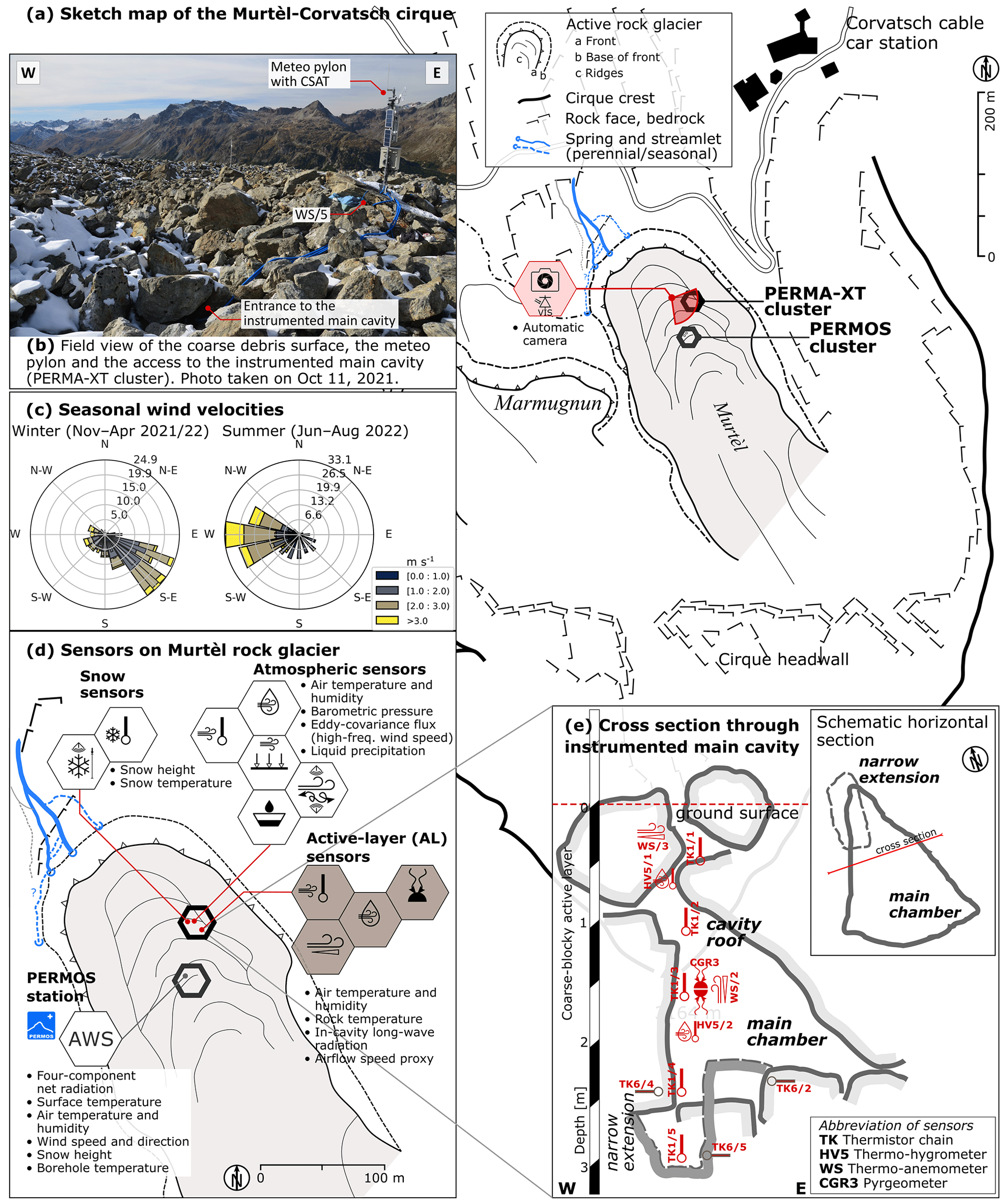
Figure 2 Sketch map of Murtèl–Corvatsch cirque (a) with two active rock glaciers, Murtèl and Marmugnun. (b) Photo of the above-surface PERMA-XT installations. (c) Wind patterns are seasonally varying in the sheltered cirque. Panels (d) and (e) show locations of sensors on Murtèl rock glacier and in the instrumented main cavity, respectively (Table 1). The term “cavity roof” used throughout the text refers to the uppermost ∼ 1 m of the instrumented cavity.

Table 1 PERMA-XT sensor specifications.

Measurement range and accuracy by manufacturer/vendor. Specifications of PERMOS sensor available in Scherler et al. (2014) and Hoelzle et al. (2022). ^a CSI: Campbell Scientific, Inc. ^b Sensors in radiation shield RAD10E. ^c CSAT measures three-dimensional high-frequency sonic wind speed and derives sonic buoyancy flux. ^d Snow temperature setup and thermistor strings manufactured by Waljag GmbH. ^e Semi-quantitative airflow speed derived from measured heat flux.

3.2 Data processing

In the present work, we analysed data of 2 years from 1 September 2020 to 30 September 2022 except for the eddy-covariance data. The sonic anemometer (CSAT) was operational from 5 November 2020 onwards.

3.2.1 Surface radiation

All four components of the radiative heat fluxes at the surface – i.e. incoming and outgoing short-wave (S) and long-wave (L) radiation – were measured directly by the PERMOS micro-meteorological station with two back-to-back pairs of Kipp & Zonen CM3 pyranometers (0.3–3 µm) and CG3 pyrgeometers (5–50 µm) (Hoelzle et al., 2022). We applied the same radiation corrections as in Hoelzle et al. (2022): (1) instrumental corrections of both pyranometers with nighttime short-wave radiation measurements (pyranometer offset correction), (2) correction for snow cover of the upward-looking pyranometer ($S^{\downarrow }=S^{\uparrow }/\mathrm{0.86}$ when $S^{\uparrow }>S^{\downarrow }$), (3) Sicart et al. (2005) correction of the incoming long-wave radiation for interference with solar radiation, and (4) rejection of incoming short-wave radiation at low sun angles (if albedo exceeds unity).

3.2.2 Eddy-covariance data

We estimated the sensible turbulent flux Q_H using the eddy-covariance method, based on the covariance of vertical wind speed fluctuations w^′ and temperature fluctuations T^′, measured by a CSI CSAT (CSI CSAT3B manual, 2020) and averaged over 30 min (Foken, 2017; see Sect. 4.2.2):

$$\begin{array}{}\text{(1)}& Q_{\mathrm{H}}^{\text{eddy}}={\mathit{\rho }}_{\mathrm{a}}{C}_p\stackrel{\mathrm{‾}}{w^{\prime }{T}^{\prime }},\end{array}$$

where (ρ_aC_p) refers to the volumetric heat capacity. We calculated buoyancy fluxes from the eddy raw data (10 Hz sampling rate) using Campbell Scientific's software EasyFlux™ and following the conventional pre-processing chain (Radić et al., 2017; Fitzpatrick et al., 2017; Steiner et al., 2018). Processing steps were trend and outlier removal, despiking (Vickers and Mahrt, 1997; Foken et al., 2012), coordinate rotation using the double rotation method (Tanner and Thurtell, 1969), and spectral corrections (Moncrieff et al., 1997; Massman, 2000).

Due to the lack of fast-response moisture measurements (no high-frequency gas analyser), the eddy-covariance method yielded the sonic buoyancy flux $\stackrel{\mathrm{‾}}{w^{\prime }{T}_{\mathrm{snc}}^{\prime }}$, which, for $\left|Q_{\mathrm{H}}\right|>\left|Q_{\mathrm{LE}}\right|$, is close to but not equal to the sensible heat flux $\stackrel{\mathrm{‾}}{w^{\prime }{T}^{\prime }}$ (Liu and Foken, 2001). We assess the discrepancy using the Bowen ratio method modified by Liu and Foken (2001) based on Schotanus et al. (1983) (“SND correction”):

$$\begin{array}{}\text{(2)}& \stackrel{\mathrm{‾}}{w^{\prime }{T}^{\prime }}=\stackrel{\mathrm{‾}}{w^{\prime }{T}_{\mathrm{snc}}^{\prime }}{\left(\mathrm{1}+{\displaystyle \frac{\mathrm{0.51}{\stackrel{\mathrm{‾}}{T}}_{\mathrm{a}}{C}_p}{L_{\mathrm{v}}\mathit{Bo}}}\right)}^{-\mathrm{1}},\end{array}$$

where T_snc is the sonic temperature, ${\stackrel{\mathrm{‾}}{T}}_{\mathrm{a}}$ is the air temperature (averaged over 30 min), and Bo refers to the Bowen ratio (Sect. 4.2.2). C_p and L_v are constants defined in Sect. 4.2.2.

3.2.3 Snow height and snow water equivalent

We measured snow height with a sonic distance sensor (Table 1) on a rock glacier ridge in addition to the nearby PERMOS snow height measurements. Raw measurements were compensated for variations in the speed of sound with air temperature, following the manufacturer's guidelines (CSI SR50A manual, 2020).

We used the semi-empirical ΔSNOW model (Winkler et al., 2021) to convert the measured snow height to snow water equivalent (SWE). This parsimonious model requires snow height and its temporal changes as the sole input. Calibration data used to develop their model were gathered in the Swiss and Austrian Alps in climatic regions similar to the Engadine.

3.2.4 Precipitation

We measured liquid precipitation with an unheated tipping-bucket rain gauge (Table 1) mounted on a rock glacier ridge.

Snow or sleet (a mix of snow and rain) can fall in any month of the year. The distinction from rain is important because of the latent heat of melting L_m that ice carries and by far exceeds the sensible heat of rainwater (c_wΔT). In the comparatively dry climate of the Engadine, wet-bulb temperature can be a better discriminator than dry-bulb temperature (Froidurot et al., 2014). Wet-bulb temperature T_wb [K] is defined in Stull (2017):

$$\begin{array}{}\text{(3)}& e-e^{\ast }\left(T_{\mathrm{wb}}\right)=-\mathit{\gamma }(T-T_{\mathrm{wb}})\left[\mathrm{Pa}\right],\end{array}$$

where $\mathit{\gamma }=\left(c_{\mathrm{p}}P\right)/\left(\mathrm{0.622}{L}_{\mathrm{v}}\right)$ [Pa K⁻¹] is the psychrometric “constant”. Equation (3) is solved iteratively. Based on hourly images from the automatic time-lapse camera, we defined a conservative wet-bulb temperature threshold of 2 °C that separates snow or sleet (T_wb<2 °C) from rain.

3.2.5 Sub-surface long-wave radiation

The in-cavity net long-wave radiation $Q_{\mathrm{CGR}\mathrm{3}}^{\mathrm{rad}}$ was calculated from the upwards $L_{\mathrm{al}}^{\uparrow }$ and downwards $L_{\mathrm{al}}^{\downarrow }$ long-wave radiation components measured with a back-to-back pyrgeometer pair installed in the instrumented cavity at a depth of 1.55 m beneath ground level (Table 1):

$$\begin{array}{}\text{(4)}& Q_{\mathrm{CGR}\mathrm{3}}^{\mathrm{rad}}=(L_{\mathrm{al}}^{\uparrow }-L_{\mathrm{al}}^{\downarrow }),\end{array}$$

which is not to be confused with the long-wave radiation L measured at 2 m a.g.l. (Sect. 4.2.1).

We corrected raw outputs $L_{\mathrm{raw}}^{\uparrow /\downarrow }$ from the two pyrgeometers in the instrumented cavity by accounting for the long-wave radiation emitted by the instruments themselves (Kipp & Zonen CGR3 manual, 2014):

$$\begin{array}{}\text{(5)}& L_{\mathrm{al}}^{\uparrow /\downarrow }=L_{\mathrm{raw}}^{\uparrow /\downarrow }+\mathit{\sigma }{T}_{\text{CGR3}}^{\mathrm{4}},\end{array}$$

where T_CGR3 refers to the pyrgeometer housing temperature. Large (>0.5 °C) or rapid changes in housing temperature differences between the two back-to-back mounted pyrgeometers indicated dust or water deposition on the upward-facing pyrgeometer window. Such disturbed measurements appeared in the high-resolution (10 min) data but did not significantly affect the daily net long-wave radiation balance in the sheltered cavity.

3.2.6 Sub-surface airflow speed

We refer to the sub-surface “wind” in the cavity as “airflow” to differentiate it from the atmospheric wind. We used the Hukseflux WS01/TP01 sensor to perform airflow speed measurements in the AL cavities. This sensor included a heated foil that measures a cooling rate expressed as a convective heat transfer coefficient h_WS [$\mathrm{W}{\mathrm{m}}^{-\mathrm{2}}{\mathrm{K}}^{-\mathrm{1}}$] related to airflow speed (Hukseflux WS01 manual, 2006). We did not convert h_WS to airflow speed but process this variable as a semi-quantitative indicator assuming u∝h_WS, sufficient for our purpose. WS01/TP01 do not resolve the direction of the airflow (hence the term “speed” instead of “velocity”). Deposition and evaporation of liquid water can disturb measurements (h_WS increase), as revealed by wrapping the heated foils in moist tissues. WS01 measurements during precipitation events were filtered out. Repeated zero-point checks were performed throughout the snow-free season by enclosing the heated foil in small, dry plastic bags for a few hours, ensuring stagnant conditions with zero airflow speed. Neither drift nor temperature dependency beyond measurement uncertainty was detected.

4 Surface energy balance calculation

4.1 Energy balance of the Murtèl near-surface AL

The point-scale surface energy balance at seasonally snow-covered sites accounts for net radiation Q^∗ [W m⁻²], composed of short- and long-wave radiation components; turbulent fluxes, composed of sensible heat Q_H [W m⁻²] and latent heat Q_LE [W m⁻²]; melt energy of snow Q_M at the surface [W m⁻²]; energy from precipitation Q_P [W m⁻²]; and heat flux Q_G [W m⁻²] into and from the ground when snow-free, replaced by conductive heat flux across the snow cover Q_S [W m⁻²] when snow covered:

$$\begin{array}{}\text{(6)}& \begin{array}{rl}& \underset{\text{net radiation}{Q}^{\ast }}{\underbrace{S^{\downarrow }+S^{\uparrow }+L^{\downarrow }+L^{\uparrow }}}+\underset{\text{turbulent fluxes}}{\underbrace{Q_{\mathrm{H}}+Q_{\mathrm{LE}}}}+Q_{\mathrm{M}}+Q_{\mathrm{P}}+Q_{\mathrm{G}/\mathrm{S}}\\ & =\mathrm{0}\left[\mathrm{W}{\mathrm{m}}^{-\mathrm{2}}\right].\end{array}\end{array}$$

Fluxes are counted as positive if these provide energy to the reference surface, i.e. the terrain or snow surface. Unlike Scherler et al. (2014), we consider the reference surface as an infinitely thin skin layer without storage. Fluxes must be balanced at all times (Eq. 6). Ground Q_G and snow Q_S heat fluxes measured beneath the surface are extrapolated to the reference surface by means of the calorimetric correction.

4.2 Flux parameterisations

We estimated the fluxes (terms in Eq. 6) as follows: all radiative fluxes were derived from on-site measurements, i.e. net radiation Q^∗ both above the surface (PERMOS data) and within the AL (PERMA-XT data); turbulent fluxes Q_H and Q_LE were estimated using the Bowen energy balance and the bulk aerodynamic methods and directly from eddy-covariance measurements. Snowmelt Q_M and precipitation Q_P heat fluxes were estimated using the calorimetric method from SWE estimates and on-site measured rainfall rates, respectively. The heat flux in the snowpack Q_S is the calorimetrically corrected conductive heat flux at the base of the snowpack. The ground heat flux Q_G (flux in the near-surface AL) was estimated analogously to the calorimetrically corrected net long-wave radiation measured in situ in the AL at 1.5 m depth.

4.2.1 Surface radiative fluxes

The net radiation Q^∗ is the sum of the measured and corrected radiation components (Sect. 3.2.1):

$$\begin{array}{}\text{(7)}& Q^{\ast }=\underset{S^{\ast }}{\underbrace{S^{\downarrow }+S^{\uparrow }}}+\underset{L^{\ast }}{\underbrace{L^{\downarrow }+L^{\uparrow }}},\end{array}$$

where S^↑ is the outgoing short-wave radiation, S^↓ is the incoming short-wave radiation, and net short-wave radiation S^∗ is the sum of both; correspondingly, L^↑ represents the outgoing long-wave radiation, L^↓ is the incoming long-wave radiation, and net long-wave radiation L^∗ is the sum of both.

4.2.2 Surface turbulent heat fluxes Q_H, Q_LE

We estimated the turbulent flux using three different methods: (1) the Bowen energy balance method (Bowen, 1926), (2) the bulk aerodynamic method (Mittaz et al., 2000; Hoelzle et al., 2022), and (3) directly with the eddy-covariance method from CSAT measurements (in the lack of a fast-response vapour analyser, only the sensible turbulent flux Q_H is estimated; Sect. 3.2.2).

Bowen energy balance method

The Bowen ratio Bo is defined as the ratio of sensible to latent heat flux (Bowen, 1926; Ohmura, 1982; Oke, 1987) and reflects the partitioning of the turbulent fluxes into sensible and latent components:

$$\begin{array}{}\text{(8)}& \mathit{Bo}:={\displaystyle \frac{Q_{\mathrm{H}}}{Q_{\mathrm{LE}}}}={\displaystyle \frac{K_{\mathrm{h}}}{K_{\mathrm{w}}}}{\displaystyle \frac{C_p\mathrm{\Delta }T}{L_{\mathrm{v}}\mathrm{\Delta }q}}\approx {\displaystyle \frac{C_p(T_{\mathrm{a}}-T_{\mathrm{s}})}{L_{\mathrm{v}}(q_{\mathrm{a}}-q_{\mathrm{s}})}},\end{array}$$

where K_h represents the eddy diffusivities for sensible heat and K_w is water vapour. Invoking the similarity principle and assuming K_h≈K_w (Ohmura, 1982), the Bowen ratio can be calculated from the isobaric specific heat capacity of air ($C_p=C_{\mathrm{pd}}(\mathrm{1}+\mathrm{0.84}q)$ with C_pd=1005 $\mathrm{J}{\mathrm{kg}}^{-\mathrm{1}}{\mathrm{K}}^{-\mathrm{1}}$) (Reid and Brock, 2010; Hoelzle et al., 2022), the latent heat of vaporisation L_v (if T_s≥0 °C) or sublimation L_s (if T_s<0 °C) (2.48×10⁶ J kg⁻¹, 2.83×10⁶ J kg⁻¹), and the gradients of temperature ΔT and specific humidity Δq (specified below). The sensible and latent turbulent fluxes are then expressed as a function of the available energy $Q^{\ast }+Q_{\mathrm{M}}+Q_{\mathrm{G}/\mathrm{S}}$ (Q_P considered negligible; Sect. 5.3.4):

$$\begin{array}{}\text{(9)}& \begin{array}{rl}& Q_{\mathrm{H}}^{\mathit{Bo}}={\displaystyle \frac{Q^{\ast }+Q_{\mathrm{M}}+Q_{\mathrm{G}/\mathrm{S}}}{\mathrm{1}+\mathrm{1}/\mathit{Bo}}},\\ & Q_{\mathrm{LE}}^{\mathit{Bo}}={\displaystyle \frac{Q^{\ast }+Q_{\mathrm{M}}+Q_{\mathrm{G}/\mathrm{S}}}{\mathrm{1}+\mathit{Bo}}}.\end{array}\end{array}$$

The ground and snow surface temperature T_s [°C] was calculated from the measured long-wave radiation components L and the Stefan–Boltzmann law via (Oke, 1987)

$$\begin{array}{}\text{(10)}& \mathit{\epsilon }\mathit{\sigma }{T}_{\mathrm{s}}^{\mathrm{4}}=L^{\uparrow }-(\mathrm{1}-\mathit{\epsilon })L^{\downarrow },\end{array}$$

where ε is the surface emissivity; σ represents the Stefan–Boltzmann constant ($\mathit{\sigma }=\mathrm{5.670}\times {\mathrm{10}}^{-\mathrm{8}}$ $\mathrm{W}{\mathrm{m}}^{-\mathrm{2}}{\mathrm{K}}^{-\mathrm{4}}$); and L^↑ and L^↓ represent the measured outgoing and incoming long-wave radiation, respectively. We took the emissivity value of ε=0.96 from Scherler et al. (2014).

The surface specific humidity q_s [g g⁻¹] is either the specific humidity of the air in the near-surface coarse blocky AL q_sa (measured) or the saturated snow surface $q_{\mathrm{ss}}^{\ast }(T_{\mathrm{s}},P_{\mathrm{a}})$, depending on whether or not the snow cover is thick enough to suppress convective air exchange between the AL and the atmosphere (Sect. 6.3.1).

$$\begin{array}{}\text{(11)}& q_{\mathrm{s}}=\left\{\begin{array}{ll}{q}_{\mathrm{sa}},& \text{for}{h}_{\mathrm{S}}{\le }^{\text{SEB}}{\widehat{h}}_{\mathrm{S}}^{\text{crit}}\text{(snow-free or open snow cover)}\\ q_{\mathrm{ss}}^{\ast },& \text{for}{h}_{\mathrm{S}}{>}^{\text{SEB}}{\widehat{h}}_{\mathrm{S}}^{\text{crit}}\text{(decoupling snow cover)}\end{array}\right.\end{array}$$

The critical snow height ${}^{\text{SEB}}{\widehat{h}}_{\mathrm{S}}^{\text{crit}}$ is reached when the AL is so strongly decoupled from the atmosphere that the convective fluxes across the snow cover are no longer detectable by our SEB estimations. We determine the snow height ${}^{\text{SEB}}{\widehat{h}}_S^{\text{crit}}$ using the AL air temperature, specific humidity, and airflow speeds (Sect. 6.3.1). The specific humidity of the air q_a was calculated from the measured air temperature T_a and relative humidity at the measurement level z_m of 2 m a.g.l.

Bulk aerodynamic method

In the bulk parameterisation, sensible $Q_{\mathrm{H}}^{\text{bulk}}$ and latent $Q_{\mathrm{LE}}^{\text{bulk}}$ turbulent fluxes are driven by the gradients of temperature $\mathrm{\Delta }T=T_{\mathrm{a}}-T_{\mathrm{s}}$ [K, °C] and specific humidity $\mathrm{\Delta }q=q_{\mathrm{a}}-q_{\mathrm{s}}$ [g g⁻¹], respectively, and horizontal wind speed u [m s⁻¹]:

$$\begin{array}{}\text{(12)}& {\displaystyle }{Q}_{\mathrm{H}}^{\text{bulk}}& {\displaystyle }={\mathit{\rho }}_{\mathrm{a}}{C}_{p}u(T_{\mathrm{a}}-T_{\mathrm{s}})C_{\mathrm{bt}},\text{(13)}& {\displaystyle }{Q}_{\mathrm{LE}}^{\text{bulk}}& {\displaystyle }={\mathit{\rho }}_{\mathrm{a}}{L}_{\{\mathrm{v},\mathrm{s}\}}u(q_{\mathrm{a}}-q_{\mathrm{s}})C_{\mathrm{bt}},\end{array}$$

where ρ_a [kg m⁻³] represents air density. The flux–gradient relationship is modified by atmospheric stability, accounting for enhanced turbulent fluxes in an unstable atmosphere and suppressed turbulent fluxes in a stable atmosphere, by means of the bulk exchange factors C_bt (bulk turbulent heat and vapour transfer coefficients) [unitless, –]. Different formulations of the stability functions exist. Here, we use the modified Louis (1979) scheme (Song, 1998), motivated by its use in the GEOtop model, a distributed hydrological model designed for complex terrain (Rigon et al., 2006; Endrizzi et al., 2014), and other studies (e.g. Essery and Etchevers, 2004). We compare the modified Louis (1979) scheme with the iterative Monin–Obukhov scheme and the widely used Businger–Dyer scheme (Oke, 1987). The latter has been used in the previous SEB studies on Murtèl by Mittaz et al. (2000) and Scherler et al. (2014) and in many SEB estimates on debris-covered glaciers (Brock et al., 2010; Reid and Brock, 2010; Reid et al., 2012; Steiner et al., 2018, 2021), despite discrepancies (overestimated fluxes) at strongly unstable atmosphere noted by Steiner et al. (2018). The issue with the Businger–Dyer parameterisation is that near-surface wind speeds on topographically sheltered rough terrain tend to be lower for a given atmospheric stability compared with the conditions under which the empirical Businger–Dyer parameterisation was originally developed (flatland in Kansas, USA; Businger et al., 1971; Haugen et al., 1971). This approach is therefore problematic in complex terrain, including our study site. Finally, we test the parameterisation without stability correction (“bulk c0”), which corresponds to the special case of a neutral atmosphere. Detailed explanations of the parameterisation schemes of the turbulent heat transfers are described in the appendix (Appendix A).

Accurate estimates of turbulent fluxes rely on representative values for the roughness lengths for momentum z_0m, heat z_0h, and moisture z_0q (Steiner et al., 2018; Smeets et al., 1999; Smith, 2014). We calculated the roughness length for momentum z_0m from the eddy-covariance data following Conway and Cullen (2013) and Fitzpatrick et al. (2017):

$$\begin{array}{}\text{(14)}& z_{\mathrm{0}\mathrm{m}}=(z_{\mathrm{u}}-d)\exp \left\{-k_{\ast }{\displaystyle \frac{{\stackrel{\mathrm{‾}}{u}}_{\mathrm{h}}}{u_{\ast }}}-{\mathit{\psi }}_{\mathrm{m}}\left({\displaystyle \frac{z_{\mathrm{u}}-d}{L}}\right)\right\},\end{array}$$

where ${\stackrel{\mathrm{‾}}{u}}_{\mathrm{h}}$ [m s⁻¹] represents the mean horizontal wind speed, u_∗ [m s⁻¹] is the friction velocity, k_∗ [0.40] is the von Kármán constant, z_u [m] is the measurement height of wind speed, L [m] is the Obukhov length, ψ is the integrated stability function (Appendix A), and d is the zero-plane displacement height. We set the (unknown) zero-plane displacement height d to zero (Miles et al., 2017). The sensor height z_u(t) is the variable distance above the ground or snow surface: $z_{\mathrm{u}}\left(t\right):=z_{\mathrm{CSAT}}-h_{\mathrm{S}}\left(t\right)$. The recommended filtering is to use only ${\stackrel{\mathrm{‾}}{u}}_{\mathrm{h}}>\mathrm{3}$ m s⁻¹ under near-neutral conditions $|z_{\mathrm{u}}/L|<\mathrm{0.05}$ (Radić et al., 2017; Nicholson and Stiperski, 2020). We compared our eddy-covariance-derived roughness length for momentum z_0m with the aerodynamically derived values reported in Mittaz et al. (2000). For simplicity, the scalar lengths for heat z_0h and humidity z_0q are often considered equal to the momentum roughness length z_0m (Sicart et al., 2005; Reid and Brock, 2010) or 1–3 orders of magnitudes smaller (Smeets and van den Broeke, 2008). Here, we could not independently estimate the scalar roughness lengths z_0h and z_0q due to the lack of humidity-corrected sonic temperature or high-frequency humidity measurements. We assumed an equal roughness length for heat and moisture, z_0h=z_0q, and used the unknown ratio ${\widehat{R}}_{z\mathrm{0}}:=z_{\mathrm{0}\mathrm{h}}/z_{\mathrm{0}\mathrm{m}}=z_{\mathrm{0}q}/z_{\mathrm{0}\mathrm{m}}$ as a calibration parameter.

Finally, we compared the sensible turbulent flux with the katabatic model of Oerlemans and Grisogono (2002) specifically developed for conditions of katabatic or nocturnal drainage winds. This is different from all the above-mentioned parameterisations as this predicts a quadratic rather than near-linear relation between Q_H and the driving temperature difference ΔT. Since we lacked vertical profile observations of potential temperature required for this parameterisation, we could not test this bulk method. Instead, we checked the validity of the quadratic Q_H–ΔT relation on Murtèl (cf. Radić et al., 2017) and show wind profile measurements collected by Mittaz et al. (2000) in the years 1997–2000 (Appendix D).

4.2.3 Snowmelt heat flux Q_M, snow heat flux Q_S, and snowpack sensible heat storage H_S

The snowmelt heat flux Q_M is the heat flux consumed by the melting snowpack. We estimated Q_M from the daily change in SWE [kg m⁻²] derived from the snow height data h_S (sonic ranger data) with the semi-empirical parsimonious ΔSNOW model (Winkler et al., 2021):

$$\begin{array}{}\text{(15)}& Q_{\mathrm{M}}\approx L_{\mathrm{m}}{\displaystyle \frac{\mathrm{\Delta }\left(\text{SWE}\right)}{\mathrm{\Delta }t}},\text{ if }{T}_{\mathrm{b}}=\mathrm{0}\mathrm{°}\mathrm{C},\end{array}$$

where L_m [336 kJ kg⁻¹] represents the latent heat of fusion for ice. We considered runoff-generating snowmelt to occur in spring when temperature at the base of the snowpack T_b reaches the melting point and ignored melting–refreezing events within the snowpack.

The snow heat flux Q_S is the conductive heat flux across the single-layer snowpack. We calculated ${\stackrel{\mathrm{̃}}{Q}}_{\mathrm{S}}$ in the lowermost 25 cm of the snowpack, ignoring transient effects (Mittaz et al., 2000):

$$\begin{array}{}\text{(16)}& \begin{array}{rl}{\stackrel{\mathrm{̃}}{Q}}_{\mathrm{S}}& =-k_{\mathrm{S}}{\displaystyle \frac{\mathrm{d}T}{\mathrm{d}z}}\approx -k_{\mathrm{S}}{\displaystyle \frac{T_{\mathrm{s}}-T_{\mathrm{b}}}{h_{\mathrm{S}}}}\approx -k_{\mathrm{S}}{\displaystyle \frac{T_{\mathrm{25}}-T_{\mathrm{0}}}{\mathrm{\Delta }z}},\\ & \text{ if }{h}_{\mathrm{S}}>\mathrm{30}\mathrm{cm}\text{and}\mathrm{0}\text{otherwise},\end{array}\end{array}$$

where $\mathrm{d}T/\mathrm{d}z$ is a linearised temperature gradient in the lowermost 25 cm of the snowpack. To ensure that both thermistors are snow covered, the minimum snow height h_S required is 30 cm. We related the snow thermal conductivity k_S to the snow density via the empirical equation $k_{\mathrm{S}}:=k_{\mathrm{S}}\left({\mathit{\rho }}_{\mathrm{S}}\right)=\mathrm{2.93}({\mathrm{10}}^{-\mathrm{6}}{\mathit{\rho }}_{\mathrm{S}}^{\mathrm{2}}+{\mathrm{10}}^{-\mathrm{2}})$ developed for Murtèl (Keller and Gubler, 1993; Hoelzle et al., 2022), where we estimated the bulk density of the snowpack with the ΔSNOW model via ${\stackrel{\mathrm{‾}}{\mathit{\rho }}}_{\mathrm{S}}=\text{SWE}/h_{\mathrm{S}}$ (Winkler et al., 2021).

${\stackrel{\mathrm{̃}}{Q}}_{\mathrm{S}}$ was calculated near the base of the snowpack instead of at the snow reference surface to which Eq. (6) refers. With this approach, we used the more stable snow density and thermal conductivity near the snowpack base, which is less affected by compaction than the near-surface layers that receive fresh snow. The heat flux ${\stackrel{\mathrm{̃}}{Q}}_{\mathrm{S}}$ was extrapolated to the snow surface by adding the sensible heat storage changes in the snowpack ΔH_S above z_S=25 cm (“calorimetric correction”) (Foken, 2008; Liebethal et al., 2005; Boike et al., 2003). We estimated the changes in cold content ΔH_S as

$$\begin{array}{}\text{(17)}& \mathrm{\Delta }{H}_{\mathrm{S}}\approx c_{\mathrm{S}}\left(m_{\mathrm{S}/\mathrm{A}}\right)\mathrm{\Delta }{T}_{\mathrm{S}}/\mathrm{\Delta }t\approx c_{\mathrm{S}}\text{SWE}\langle \mathrm{\Delta }{T}_{\mathrm{S}}\rangle /\mathrm{\Delta }t,\end{array}$$

where $\left(m_{\mathrm{S}/\mathrm{A}}\right)$ represents the mass of the snowpack per area, i.e. the SWE [kg m⁻²]; c_S [$\mathrm{2.050}\mathrm{kJ}{\mathrm{kg}}^{-\mathrm{1}}{\mathrm{K}}^{-\mathrm{1}}$] is the specific heat capacity of snow or ice at 0°C; and 〈ΔT_S〉 [°C] represents the layer-averaged snow temperature changes. The calorimetrically corrected snow heat flux Q_S was then calculated as

$$\begin{array}{}\text{(18)}& Q_{\mathrm{S}}={\stackrel{\mathrm{̃}}{Q}}_{\mathrm{S}}+\mathrm{\Delta }{H}_{\mathrm{S}}.\end{array}$$

4.2.4 Precipitation heat flux Q_P

The rainfall heat flux Q_Pr was estimated via (Sakai et al., 2004; Reid and Brock, 2010)

$$\begin{array}{}\text{(19)}& Q_{\mathrm{Pr}}=C_{\mathrm{w}}r(T_{\mathrm{P}}-T_{\mathrm{s}}),\end{array}$$

where C_w=ρ_wc_w (4.18 $\mathrm{MJ}{\mathrm{m}}^{-\mathrm{3}}{\mathrm{K}}^{-\mathrm{1}}$) is the water volumetric heat capacity and r [${\mathrm{m}}^{\mathrm{3}}{\mathrm{m}}^{-\mathrm{2}}{\mathrm{s}}^{-\mathrm{1}}$] is the rainfall rate intercepted at the surface. Precipitation temperature T_P was approximated using the wet-bulb temperature T_wb, calculated from air temperature and relative humidity (Eq. 3). We assumed precipitation in the form of rain if T_wb≥2 °C. Water contributions from upslope flowing onto the rock glacier and liquid precipitation falling into the snowpack were not accounted for.

The heat flux Q_Ps due to rapid melting of sleet or shallow summertime snow (T_wb<2 °C, h_S<10 cm) was roughly estimated as

$$\begin{array}{}\text{(20)}& Q_{\mathrm{Ps}}\sim L_{\mathrm{m}}{\mathit{\rho }}_{\mathrm{w}}{r}_{\mathrm{s}},\end{array}$$

where r_s [${\mathrm{m}}^{\mathrm{3}}{\mathrm{m}}^{-\mathrm{2}}{\mathrm{s}}^{-\mathrm{1}}$] represents the amount of solid precipitation that melts in the pluviometer per time period Δt [s]. Our measurement setup was not designed to accurately record the precipitation rate during mixed rain- and snowfall or the fraction of ice crystals and liquid water in the total precipitation. The heat flux Q_Ps is intended as an order-of-magnitude estimate.

4.2.5 Near-surface ground heat flux Q_G and sensible heat storage $H_{\mathrm{al}}^{\mathit{\theta }}$

Analogously to the calorimetrically corrected snow heat flux Q_S, the ground heat flux Q_G is the sum of the measured net long-wave radiation in the instrumented cavity $Q_{\mathrm{CGR}\mathrm{3}}^{\mathrm{rad}}$ (Eq. 4) and the sensible heat storage changes $\mathrm{\Delta }{H}_{\mathrm{al}}^{\mathit{\theta }}$ of the virtual layer between the ground surface and the depth of the pyrgeometer:

$$\begin{array}{}\text{(21)}& Q_{\mathrm{G}}=Q_{\mathrm{CGR}\mathrm{3}}^{\mathrm{rad}}+\mathrm{\Delta }{H}_{\mathrm{al}}^{\mathit{\theta }}.\end{array}$$

Rock mass subject to changing temperatures constitutes a heat source or sink (Scherler et al., 2014). The sensible heat storage change in the (dry) blocks $\mathrm{\Delta }{H}_{\mathrm{al}}^{\mathit{\theta }}$ is proportional to the rate of change in rock temperature, assuming a constant volumetric heat capacity $\partial \mathit{\left\{}\right(\mathrm{1}-{\mathit{\varphi }}_{\mathrm{al}}\left){\mathit{\rho }}_{\mathrm{r}}{c}_{\mathrm{r}}\mathit{\right\}}/\partial t=\mathrm{0}$. In the lack of rock temperatures over the 2-year time period analysed in this work, we use in-cavity air temperatures ${\stackrel{\mathrm{‾}}{T}}_{\mathrm{a}}$ averaged over a thermal adjustment timescale Δt_r (1 d) as a surrogate (Sect. 6.1.2; Appendix C). The rate of sensible heat storage and release of the blocks was then approximately calculated as (Liebethal and Foken, 2007; Ochsner et al., 2007; Brock et al., 2010)

$$\begin{array}{}\text{(22)}& \begin{array}{rl}\mathrm{\Delta }{H}_{\mathrm{al}}^{\mathit{\theta }}& =\underset{-z_{\mathrm{s}}}{\overset{\mathrm{0}}{\int }}{\displaystyle \frac{\partial }{\partial t}}\mathit{\left\{}\right(\mathrm{1}-{\mathit{\varphi }}_{\mathrm{al}}\left){\mathit{\rho }}_{\mathrm{r}}{c}_{\mathrm{r}}{T}_{\mathrm{r}}\right(z\left)\mathit{\right\}}\mathrm{d}z\\ & \approx (\mathrm{1}-{\mathit{\varphi }}_{\mathrm{al}}){\displaystyle \frac{\langle {\mathit{\rho }}_{\mathrm{r}}{c}_{\mathrm{r}}\rangle }{\mathrm{\Delta }{t}_{\mathrm{r}}}}\sum _i\mathit{\{}\langle {\stackrel{\mathrm{‾}}{T}}_{\mathrm{a}}(z_i,t+\mathrm{\Delta }{t}_{\mathrm{r}})\rangle \\ & -\langle {\stackrel{\mathrm{‾}}{T}}_{\mathrm{a}}(z_i,t)\rangle \mathit{\}}\mathrm{\Delta }{z}_i,\end{array}\end{array}$$

where z_s=155 cm is the distance from the pyrgeometer pair to the ground surface (reference level); ρ_r is the rock density (2690 kg m⁻³) (Corvatsch granodiorite; Schneider, 2014); c_r is the specific heat capacity (790 $\mathrm{J}{\mathrm{kg}}^{-\mathrm{1}}{\mathrm{K}}^{-\mathrm{1}}$); ϕ_al=0.4 (Scherler et al., 2014) is the AL porosity; and T_r(z) and T_a(z) are the vertical rock and in-cavity air temperature profile [°C], respectively. In the discretised formulation, temperatures $\langle \stackrel{\mathrm{‾}}{T}\left(z_i\right)\rangle$ are layer-wise averages in the ith layer with thickness Δz_i (denoted by “〈⋅〉”) derived from the thermistor string TK1/1 and the radiometric surface temperature T_s.

5 Results

5.1 Meteorological conditions

The weather in each season differed markedly between the 2 years analysed in the present work (2020–2022; Fig. 3). The winter 2020–2021 was colder than the 2021–2022 one (November–April: average temperature: −6.2 °C vs. −5.3 °C; minimum daily average temperature: −16.5 °C vs. −15.1 °C) and richer in terms of snow amount (November–April: average snow height measured on a wind-swept ridge: 76 cm vs. 54 cm) and duration (early onset of snow cover: 5 October vs. 3 November; later melt-out: mid-June vs. mid-May). Summer 2021 was cool and wet compared with the hot and dry summer 2022; temperatures were lower (July–August: average: 6.9 °C vs. 9.3 °C) with frequent passage of synoptic fronts, often bringing cold air (≤3 °C; minimum daily average temperature: 0.7 °C vs. 5.6 °C) and mixed precipitation (sleet). Snowfall occurred in a few days throughout the summer and melted within hours. A few snow patches survived over the summer after melt-out of the winter snowpack in mid-June. In contrast, the hot and dry summer 2022 was marked by three heat waves (in June, July, and August) and daily minimum temperatures not below 5 °C. Several dry spells occurred during this season; the longest one was an 11 d long dry spell within the 5–19 July heat wave. Almost no precipitation was recorded between 20 June and 1 August despite some convective precipitation events recorded on the nearby Piz Corvatsch cable car station (MétéoSuisse station at 3294 m a.s.l.). Discharge data of the rock glacier outflow (own measurements, not shown), camera images, and field observations (fresh debris flow deposits, flooding of furrows) revealed rainwater funnelled onto the rock glacier. Data gaps for this period were filled with MétéoSuisse precipitation data from the nearby station “Piz Corvatsch”.

Wind speeds (measured by PERMOS) in the sheltered Murtèl cirque were generally low (hourly means: 1–3 m s⁻¹; peak wind speed ∼5 m s⁻¹; Fig. 2c). The wind pattern was often marked by a strong diurnal cycle. Peak wind speed was reached during the night in winter (strong katabatic wind blowing downslope from southeast) and in the afternoon in summer (regional valley wind known as the “Maloja wind” blowing from west-northwest–west-southwest overruled a local anabatic wind). Summer nights were calm or with weak katabatic winds (wind speed: ≤2 m s⁻¹ from west–southeast).

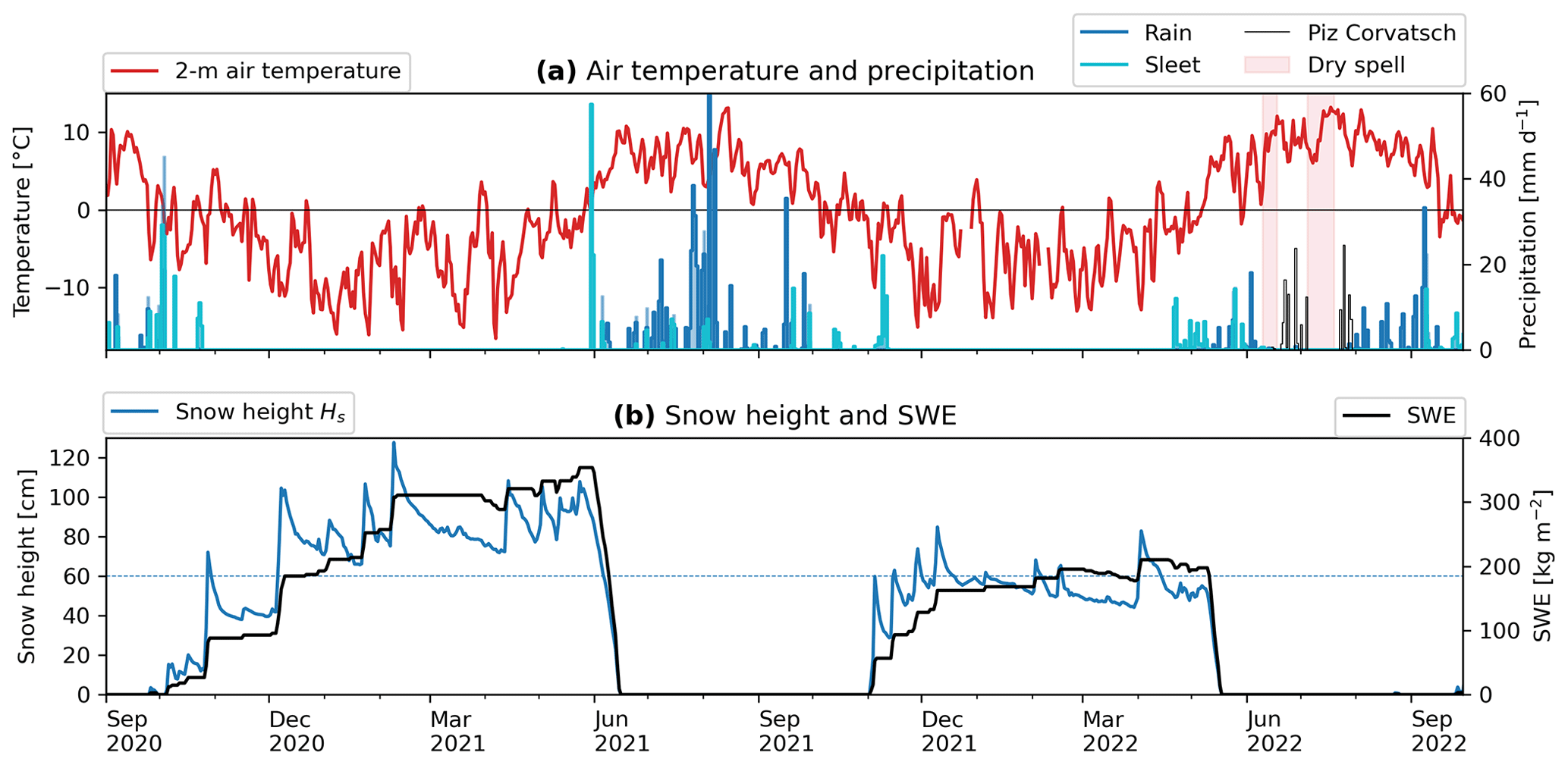
Figure 3 Meteorological conditions. (a) Air temperature (daily mean) and precipitation (daily sum). (b) Snow height and SWE. Rain and sleet (mixed precipitation) separated based on a wet-bulb temperature threshold of 2 °C. Precipitation data at Piz Corvatsch from MétéoSuisse.

5.2 Snow and ground thermo-hygric conditions

During the snow-rich winter 2020–2021, a thick and insulating snow cover (exceeding 70 cm) sealed the cavity from the atmosphere. The cavity air was kept isothermal (within ±0.2 °C; Fig. B1; Appendix B) and isohume at saturation at a much higher moisture level than that in the (colder) atmosphere (Fig. B2; Appendix B). Virtually no dry and cold air from the atmosphere was mixed into the closed cavity system. A stable winter equilibrium temperature (WEqT; bottom temperature of snow cover (BTS, Haeberli, 1973; Haeberli and Patzelt, 1982) was reached in March 2021 ($-\mathrm{4.59}\pm \mathrm{0.05}$ °C). In contrast, during the snow-poor winter 2021–2022, the rapidly fluctuating temperature and humidity (relative and specific) indicated a connection across the thin snow cover and an exchange with the dry, cold air from the atmosphere. Following snow melt-out (end of zero curtain) and re-connection with the atmosphere, the cavity air began to warm and “desaturate” from the surface downwards (July 2021; June 2022).

In summer, the near-surface cavity roof was generally warmer and more humid compared with both the atmosphere (despite slightly lower relative humidity) and the deeper cavity (specific humidity profiles are shown in Appendix Fig. B3). Daily average specific humidity in the cavity roof and that in the atmosphere were strongly correlated (R²=0.868). The near-surface cavity consistently presented a moisture surplus in relation to that of the atmosphere throughout the year. This surplus persisted even during dry spells. Summertime in-cavity temperature gradients were more stable the higher the surface temperature was. In summer 2021, frequent passages of cold fronts with rapid atmospheric cooling destabilised the in-cavity air column by reducing the temperature gradients. In summer 2022, dry spells impacted the sub-surface moisture conditions down to 2 m within 3–6 d after the last precipitation event: water infiltrated within minutes, near-surface relative humidity started to decrease within hours, and the cavity air drying front (evaporation front at the isohume of rH = 100 %) receded to greater depths within days. At a depth of 2 m, saturation was lost ∼ 5 d after the last precipitation event. Consequently, the in-cavity humidity gradients reversed, indicating a switch from downwards to upwards humidity transport. This was most pronounced in July 2022 during the intense mid-July dry spell accompanying a heat wave (Appendix Figs. B3, B2). In contrast, near the surface, the measured gradient in specific humidity between the near-surface AL and the atmosphere and, therefore, Q_LE remained largely constant regardless of the different weather conditions and the humidity gradient within the AL (Sect. 6.3.3).

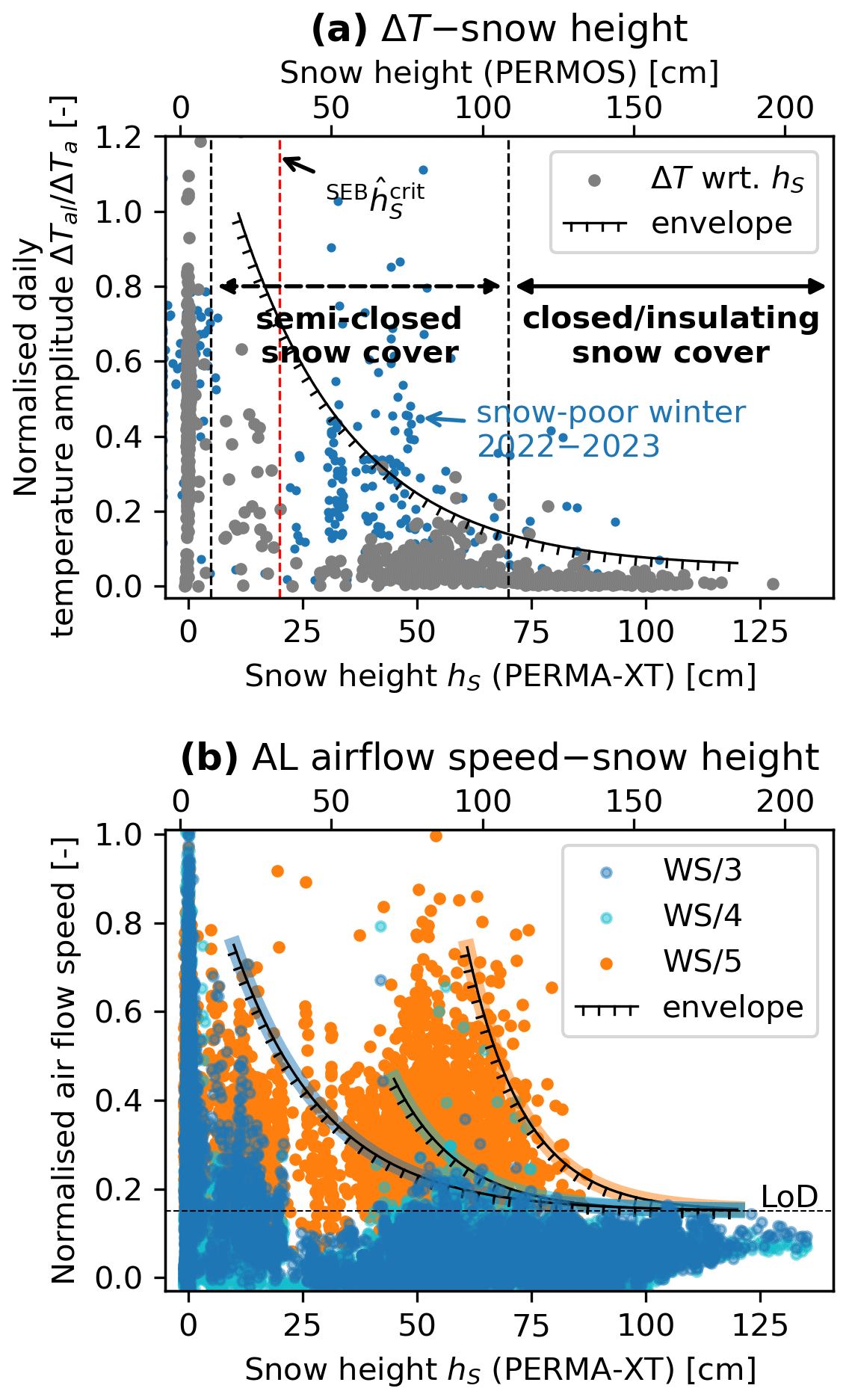
Figure 4 Indicators of AL–atmosphere coupling. (a) Relationship between the daily temperature amplitude in the cavity roof (normalised by the 2 m temperature amplitude) and the corresponding snow depth h_S measured on a wind-swept rock glacier ridge (PERMA-XT station) and a broad flat area (PERMOS station). (b) Normalised airflow speed ($u/u_{\max }$) at different locations as a proxy for sub-surface ventilation and convective coupling. Measurements below the level of detection (LoD) were considered zero. Airflow speed decreases with increasing snow height relative to the maximum speeds under snow-free conditions. Onset of decoupling varies with sensor location. WS/5 is beneath a large wind-exposed block on a ridge where snow funnels remain open longer than those on flat terrain (WS/3, WS/4).

We determine the snow height necessary to close the snow cover and to decouple the AL from the atmosphere with the sub-surface AL air temperature, specific humidity (not shown, correlated with air temperature), and airflow speeds (Fig. 4). With increasing snow depth, the differences in air temperature and specific humidity between the cavity and the atmosphere increased (Appendix Figs. B1, B2), the correlation between in-cavity and atmospheric signal was lost, and rapid (hourly–daily) fluctuations in the in-cavity temperature and specific humidity weakened (Fig. 4a). Normalised near-surface AL temperature amplitudes indicate the degree of convective coupling: amplitudes similar to that in the atmosphere mean coupled and strongly attenuated amplitudes mean decoupled (Fig. 4a; additional winter 2022–2023 data shown). The decoupling proceeded gradually with snow depth (sketched by the schematic envelope), and the thresholds are only approximate values. Also, the sub-surface airflow speed was attenuated gradually according to the micro-topographic setting that controls the local snow depth (Fig. 4b): on gently sloping and less rough terrain, the vertical connection between the coarse blocky AL and the atmosphere was reduced at snow heights of 5–20 cm and lost at ∼50–60 cm of snow (WS/3 and WS/4); on wind-swept ridges with wind erosion, a much thicker snow cover was necessary to shut down the last snow funnel (Bernhard et al., 1998; Keller and Gubler, 1993) (∼80 cm at WS/5 at the upwind side of a big block on a ridge).

5.3 Surface energy balance

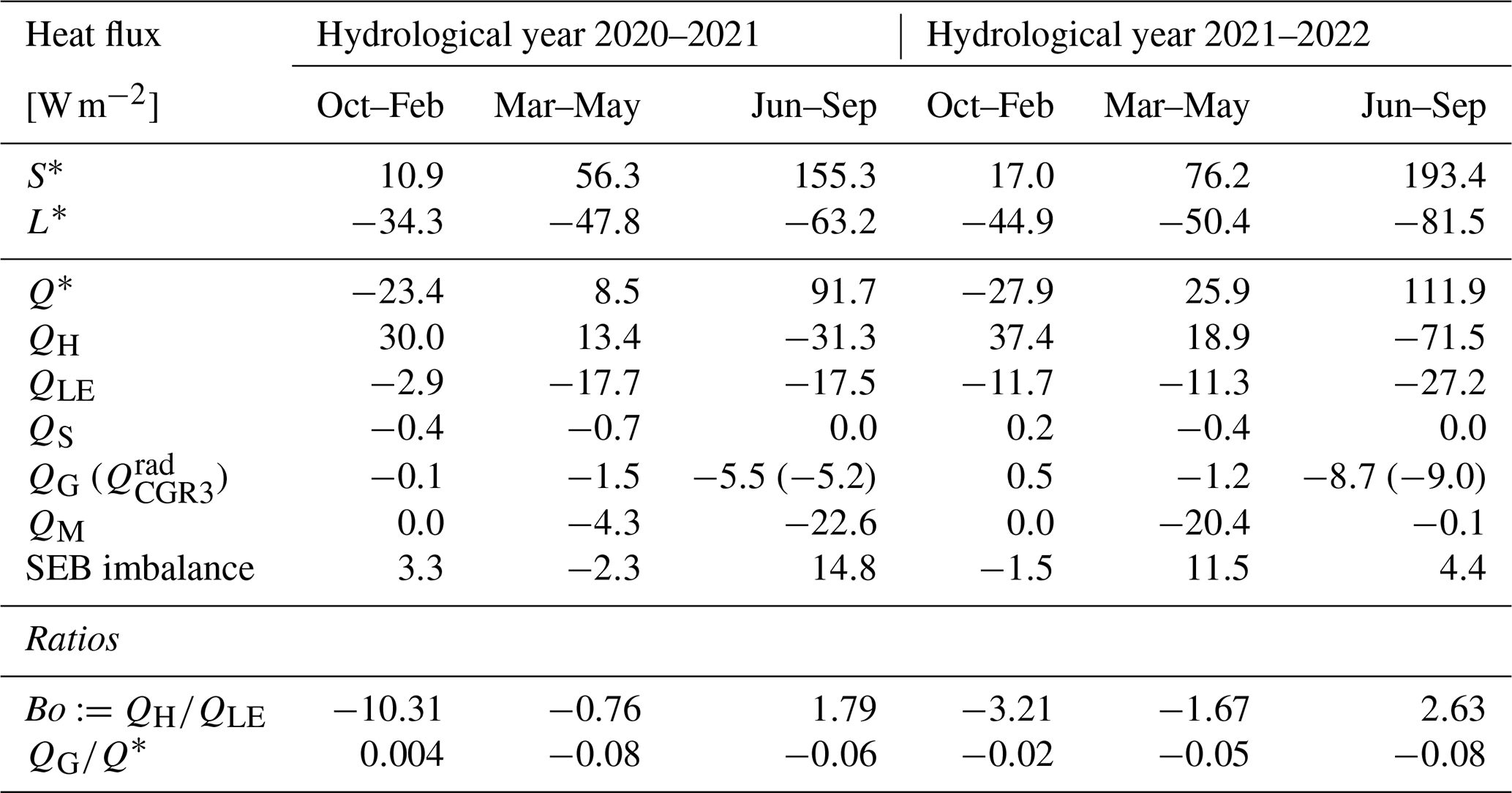
Monthly SEB (Eq. 6) is dominated by the short-wave S^∗ and long-wave L^∗ radiation components, followed by the sensible Q_H and latent Q_LE turbulent heat fluxes and the ground heat flux Q_G (Fig. 5; Table 2). In winter, turbulent fluxes compensate for the energy lost by net radiation. In summer, turbulent fluxes export roughly 90 % of the available net radiation. Snowmelt Q_M absorbs practically the entire net radiation ($Q_{\mathrm{M}}\approx -Q^{\ast }$) in the respective melt-out month (June 2021; May 2022), and the sensible and latent turbulent fluxes either are then small or roughly cancel each other (Fig. 6). The ground heat flux Q_G is downwards (negative) during snowmelt (infiltration of meltwater into the frozen coarse blocky AL releases latent heat) and net negative during the thaw season. The sensible rain heat flux Q_P is a negligible SEB component. In short, $S^{\ast }\gtrsim L^{\ast }\gg \left|Q_{\mathrm{H}}\right|>\left|Q_{\mathrm{LE}}\right|>\left|Q_{\mathrm{G}}\right|⋙Q_{\mathrm{P}}$. The parameters and constants used in the calculations are tabulated in Appendix E (Table E1).

Figure 5 (a) Monthly energy balance components. Turbulent fluxes calculated using the modified Louis (1979) parameterisation (cL^′). (b) Daily and monthly surface albedo A as a snow-cover indicator.

Table 2 Season-averaged heat fluxes and heat-flux ratios.

Turbulent fluxes calculated using the modified Louis (1979) (cL^′) bulk parameterisation.

5.3.1 Surface radiation

Short- and long-wave radiation are by far the largest SEB components (Fig. 5a). Consequently, the well-known effect of the snow cover on albedo is the single largest control of net radiation and hence of the entire SEB (Fig. 5b).

In mid-winter, the meso-scale relief controls the solar radiation budget. The shaded north-facing Murtèl cirque receives no direct insolation from November to February. Depending on cloud cover and amount of incoming diffuse or terrain-reflected short-wave radiation, the net radiation is negative and dominated by the long-wave radiation budget ($L^{\ast }\ll S^{\ast }<\mathrm{0}$). Net radiation Q^∗ was less negative in the cloudy and precipitation-rich winter 2020–2021 (December–February; average: −19 W m⁻²) than in the sunny and dry winter 2021–2022 (−40 W m⁻²) due to greater incoming long-wave radiation L^↓ emitted by the clouds (233 vs. 215 W m⁻²). A case in point is the exceptionally warm and sunny November 2020, which received in total 33 W m⁻² less short- and long-wave radiation than November 2021. The monthly mean radiation deficits are up to −53 W m⁻², which, together with the steep snow-covered slopes, is a favourable setting for strong katabatic winds.

5.3.2 Turbulent heat fluxes

The Bowen ratio partitions the available energy from net radiation, the ground heat flux, and the snowmelt heat flux into sensible and latent turbulent fluxes. Throughout the seasons of both years, the heat fluxes were as follows (Fig. 6): during wintertime, from November to March, without direct insolation in the shaded cirque, the energy loss of 20–50 W m⁻² due to long-wave emission and terrain shading was largely compensated by the sensible heat flux Q_H. Latent heat flux Q_LE at the cold snow surface was small, with mostly resublimation (moist winter 2020–2021) and sublimation fluxes (dry winter 2021–2022) within $-\mathrm{6}\pm \mathrm{10}$ W m⁻² (Fig. 6a). With the latent heat flux being small and in a variable direction, the computed Bowen ratio showed a large scatter ($\left|\mathit{Bo}\right|>\mathrm{1}$; Fig. 6b). In the drier winter 2021–2022, Q_H compensated for the heat lost by sublimation in addition to the radiative heat loss. During spring, from April to May, before the snowmelt period, the magnitude of the fluxes remained similar but the direction reversed. In summer, after complete snow melt-out, from June/July to October, the turbulent fluxes were larger to compensate for the large radiation surplus. In the more rainy summer 2021, sensible and latent heat exports were similarly large ($\mathit{Bo}=\mathrm{1.25}\pm \mathrm{2.71}$), whereas in the drier summer 2022, heat export was more dominated by sensible flux ($\mathit{Bo}=\mathrm{1.48}\pm \mathrm{2.47}$). Towards early autumn, with decreasing temperatures, the sensible flux lost importance relative to the latent flux (Bo decreased and approached zero). In September/October, with mixed precipitation (sleet) and first snow falls at still warm conditions near 0 °C, the latent heat export by sublimation from the snow cover intermittently dominated over the sensible heat uptake (Bo between 0 and −1). With further cooling, the moisture supply became limited again, and sensible heat uptake took over to offset the increasing radiation deficit ($\mathit{Bo}<-\mathrm{1}$).

We compare the estimates of turbulent fluxes (monthly averages) with the net radiation (Fig. 6) and among each other (Fig. 7). In the snow-free summer months, the Louis (1979) bulk fluxes tend to slightly underestimate the fluxes, while the Businger–Dyer fluxes (cB&D) clearly overestimate them. The measured eddy-covariance flux (buoyancy flux) falls short of closing the SEB, roughly by 50 %–75 % depending on how large the (unmeasured) eddy latent flux would be. The imbalance (“missing” flux to close the SEB; Foken, 2008) is, in any case, substantial.

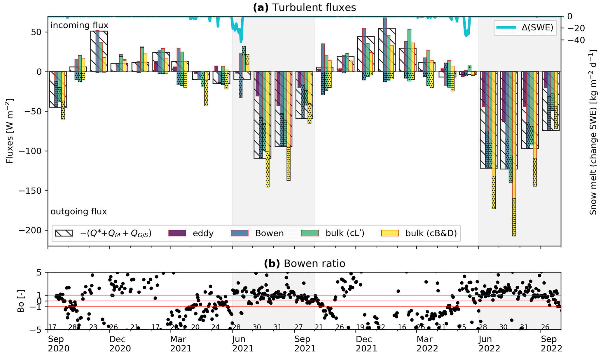
Figure 6 (a) Sensible and latent (dotted boxes) turbulent surface fluxes. Available energy from net radiation Q^∗, snowmelt Q_M, and ground heat flux Q_G (hatched boxes) is partitioned into sensible $Q_{\mathrm{H}}^{\mathit{Bo}}$ and latent $Q_{\mathrm{LE}}^{\mathit{Bo}}$ turbulent fluxes according to the Bowen ratio. The Bowen SEB is closed by design. Bulk fluxes differ according to the stability function and do not necessarily close the SEB. (b) Bowen ratio (Eq. 8). November–March: large scatter in winter because $Q_{\mathrm{LE}}^{\mathit{Bo}}$ is small and changes direction (unstable calculation). June/July–October: Bo∼ 0.5–2.5, reflecting the wet and cool summer 2021 and the dry and hot summer 2022 (Fig. 3). Monthly average based on 16–31 valid values per month.

Figure 7 Comparison of turbulent flux estimates from different parameterisations (daily and monthly averages; see Fig. 6 for time series). Comparison metrics: root mean square error (RMSE [W m⁻²]), mean bias error (MBE [W m⁻²]), and Pearson correlation coefficient (r [–]) on daily estimates.

5.3.3 Snowmelt heat flux

The latent heat of the melting snowpack Q_M largely consumes the available net radiation Q^∗ in the respective snowmelt months; the snowmelt heat flux is roughly as large as typical summer sensible turbulent heat fluxes Q_H (Fig. 5).

5.3.4 Precipitation heat flux

The sensible rain heat flux Q_Pr exerts a negligible cooling effect of $\le -\mathrm{2}$ W m⁻² at the daily timescale (not shown). Short but intense rainfall (thunderstorms) with fluxes up to −100 W m⁻² in 10 min is averaged out because such high-precipitation events are short. The heat fluxes Q_Ps arising from mixed precipitation or a shallow snow cover that melts within hours (“summer snow”; 10–30 W m⁻² daily average) are similar to Q_G and not negligible. Such events typically occur in early autumn (September–October) but also occurred throughout the wet and cool summer 2021 (June–October). Their timing often coincides with episodes of rapid ground cooling (Fig. 8).

5.3.5 Snow and ground heat fluxes

Snow heat flux Q_S is in the range of 2 to −4 W m⁻² and ground heat flux Q_G in the range of 30 to −20 W m⁻² at the daily timescale (Fig. 8). The snowpack is a thermal insulator. Within-snowpack conductive fluxes are 2–3 orders of magnitude smaller than typical SEB components. The conductive snow heat flux is negligible compared with the overall SEB and across-snowpack convective fluxes (snow funnels; Figs. 8, 4). The simplifications from the single-layer snowpack that ignore vertically varying snow density do not detract from this finding.

Heat storage changes in the snowpack (Fig. 8a) and uppermost coarse blocky AL (Fig. 8b) are asymmetric (Guodong et al., 2007) in opposite directions. In the snowpack, downwards heat transfer or warming (storage gain) is more intense (larger maxima) but less frequent, likely due to non-conductive fluxes from refreezing meltwater (synchronised with warm spells T_a>0 °C or rapid warming to the zero curtain). In the near-surface AL, upwards heat transfer or cooling (storage loss) is more intense but less frequent. Different weather conditions in the two summers analysed are reflected by Q_G: the passage of cold fronts in summer 2021 led to more frequent convective cooling, often accompanied and enhanced by sleet; conversely, ground warming is pronounced during dry spells in summer 2022. Similarly for the two winters, virtually no storage changes (Q_G≈0) occurred in the snow-rich winter 2020–2021, whereas temperature and sensible heat storage fluctuations continued in the snow-poor winter 2021–2022, albeit strongly attenuated compared with those in the snow-free season (Fig. 4; Sect. 6.3.1). The non-zero Q_G in winter 2021–2022 beneath the thin snow cover reflects convective heat exchange across the snow funnels since the conductive snow heat flux Q_S is too small to account for Q_G.

Figure 8 (a) Snow heat flux Q_S and changes in cold content of the snowpack ΔH_S. (b) Ground heat flux Q_G, net long-wave radiation in the instrumented cavity $Q_{\mathrm{CGR}\mathrm{3}}^{\mathrm{rad}}$, and sensible heat storage changes $\mathrm{\Delta }{H}_{\mathrm{al}}^{\mathit{\theta }}$ (uppermost 1.5 m of the coarse blocky AL). Beneath the insulating snow cover in winter 2020–2021, the ground thermal regime is stable, and Q_G≈0 W m⁻². In contrast, the rapid fluctuations in Q_G during the snow-poor winter 2021–2022 are faster than those during the conduction time, indicating convective processes as a driver. Heat input was larger in summer 2022 than in summer 2021.

5.4 Aerodynamic roughness length

Valid values of roughness length for momentum z_0m (Eq. 14) scatter over 2 orders of magnitude in the range of 10⁻² to 10⁰ m. Few (2.1 %) data points met the quality criteria $u_{\ast }>\mathrm{0.1}$ m s⁻¹ under near-neutral conditions $\left|\mathit{\zeta }\right|<\mathrm{0.05}$ or $\stackrel{\mathrm{‾}}{u}>\mathrm{3.0}$ m s⁻¹ (Radić et al., 2017; Nicholson and Stiperski, 2020) (Fig. 9a). The bin-wise average (median) is 0.19 m (0.23 m) for snow-free conditions (h_S<10 cm) and slightly decreases with increasing snow height up to 0.07 m (0.08 m) at 90–100 cm of snow (Fig. 9b). Averages were calculated from the average of the logarithmised values (Radić et al., 2017). Snow heights between 10 and 50 cm or exceeding 100 cm are rarely observed in the 2-year data set, hence the observation gap. z_0m is itself a function of sensor distance and hence of snow height h_S (Eq. 14). To control for possible spurious correlation in the z_0m–h_S relation, we eliminated the confounding variable h_S and tested with the constant measurement height z_CSAT=3.78 m. This did not significantly affect the z_0m–h_S relation.

Figure 9 Calculated momentum roughness length z_0m vs. (a) horizontal wind speed ${\stackrel{\mathrm{‾}}{u}}_{\mathrm{h}}$ and (b) snow height h_S. Of all values (grey dots), 2.1 % met the quality criteria (blue dots). Momentum roughness length decreases from 0.19 to 0.07 m ($\times {\mathrm{10}}^{-\mathrm{0.43}}$) with snow height increasing from 0 to 100 cm.

6 Discussion

6.1 Surface fluxes and uncertainties

6.1.1 Fluxes

Monthly SEBs are closed within the calculation uncertainties of ≤20 W m⁻² (Fig. 10, blue bars; Table 3). This represents a substantial improvement compared with Mittaz et al. (2000) and Scherler et al. (2014) and is due to the novel sensor array used in the present work. The largest SEB imbalances (deviation from closure) occur during the transition between seasons, when ground thermal conditions linger around 0 °C, during extreme meteorological conditions, and in mid-winter (December–March). These are the snowmelt months (June 2021, May 2022), early autumn (September), and the July 2022 heat wave and accompanying dry spell that strongly impacted the ground thermal and moisture regime (Figs. B1–B2). Larger deviations that occurred in the snow-rich mid-winter 2020–2021 are reduced by a “katabatic wind correction” for the variable anemometer height above the snow surface (Sect. 6.2).

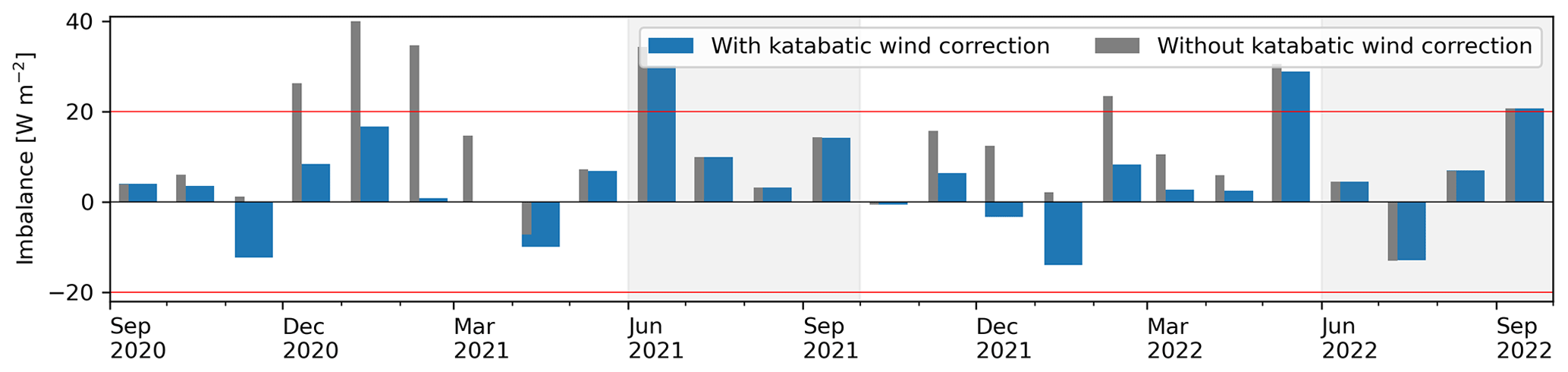
Figure 10 SEB imbalance (monthly averages). Turbulent fluxes calculated using modified Louis (1979) (cL^′) bulk parameterisation. Correcting excessively high wind speed measured in the low-level katabatic jet at thick snow cover improves the SEB in the snow-rich winter 2020–2021 (katabatic wind correction; Sect. 6.2, Eq. 23).

6.1.2 Parameter sensitivity

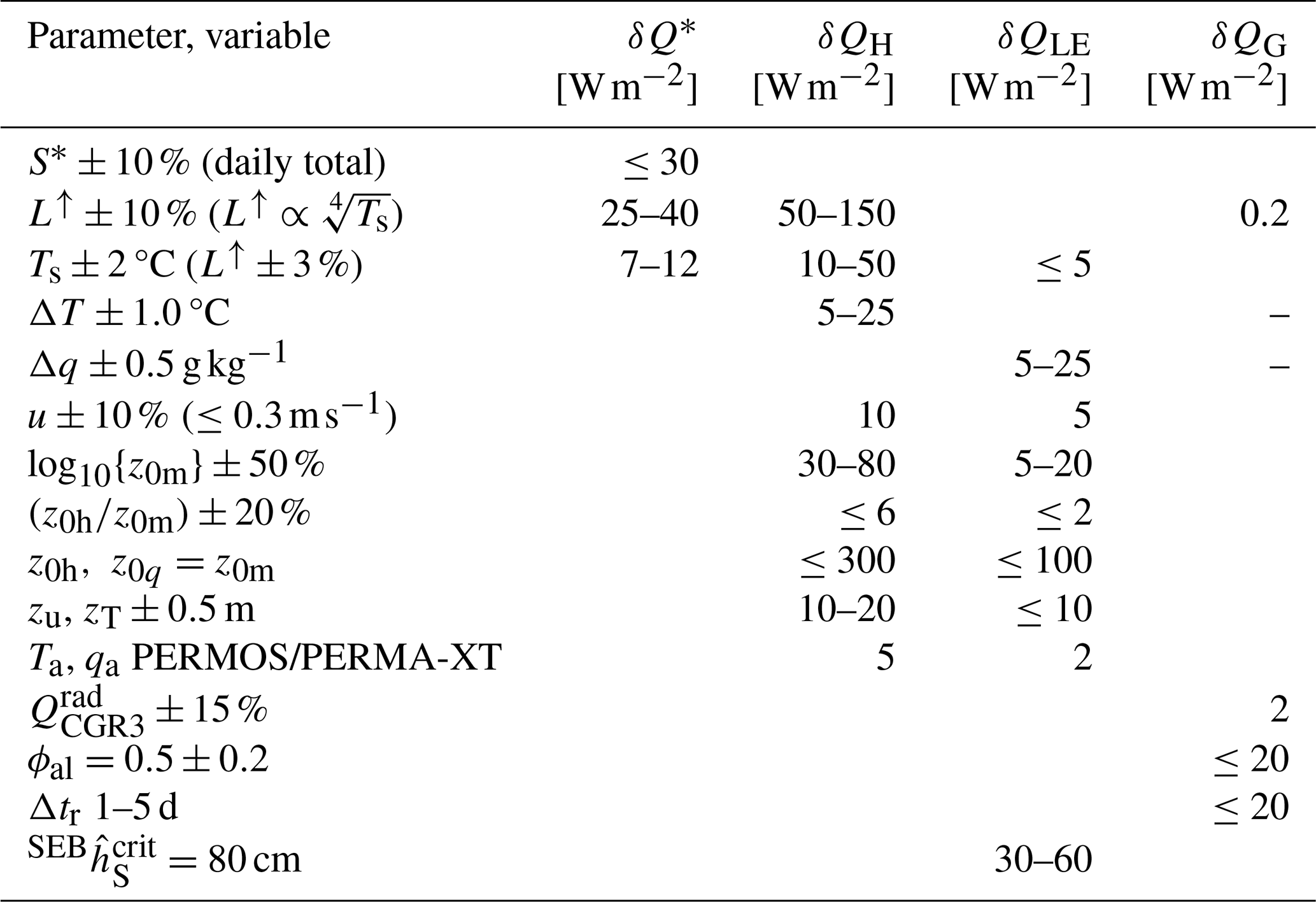
Uncertainties arise from terrain or snow cover variability across the rock glacier, spatially variable properties of the coarse blocky AL (e.g. emissivity, porosity, intrinsic permeability), and instrumental measurement errors, among other factors. We assessed the impact of the largest sources of parameter uncertainty of the heat fluxes (Table 3; sensor accuracy from Scherler et al., 2014; Hoelzle et al., 2022). We estimate our overall accuracy as ∼20 W m⁻² at the daily timescale due to uncertainties in Q_G (uncertainties in sensible heat storage changes $\mathrm{\Delta }{H}_{\mathrm{al}}^{\mathit{\theta }}$) and Q_H (uncertainty in surface temperature T_s propagated from the emissivity ε; Eq. 10). These uncertainties play an important role in this study. The SEB uncertainties determine which processes are included in the SEB estimates and which are not, complementing measurement-driven criteria. We consider insignificant (i.e. within the uncertainty) the processes with associated fluxes smaller than our 20 W m⁻² uncertainty threshold. The processes considered insignificant in the context of the SEB are not necessarily insignificant at depth. In fact, in the AL, all daily-averaged sub-surface heat fluxes are within 20 W m⁻² (Fig. 8b). We apply this criterion on the nocturnal Balch ventilation (Sect. 6.3.2) and the decoupling snow height ${}^{\text{SEB}}{\widehat{h}}_{\mathrm{S}}^{\text{crit}}$ (Sect. 6.3.3).

Insolation differences due to the local shading effect of the coarse terrain surface, the terrain slope effects, or instrumental effects (cosine response) might lead to differences of up to 30 W m⁻² (daily average) in summer (Table 3) (Otto et al., 2012; Scherler et al., 2014; Fitzpatrick et al., 2017; Kraaijenbrink et al., 2018). Uncertainties in the outgoing long-wave radiation L^↑ of ±10 % corresponding to a radiometric surface temperature difference of 7 °C might arise from patchy snow cover. The lateral advective heat transport altering the boundary layer characteristics (Essery et al., 2006; Mott et al., 2013, 2015) could explain the large SEB imbalance (Fig. 5) of roughly 100–150 W m⁻² during the melt-out phase. Smaller but still significant T_s differences of 2 °C can occur due to local shading (micro-topography) or uncertainty in emissivity (e.g. variable snow emissivity; Steiner et al., 2018) and lead to considerable Q_H uncertainties of up to 50 W m⁻². Surface temperature differences from different emissivity values (ε=1 instead of 0.96 from Scherler et al. (2014); Eq. 10) are within −1.2 and +0.25 °C. The deviations tend to be largest on hot clear-sky days with little incoming long-wave radiation L^↓ (Eq. 10) and hence might translate into considerable uncertainties in Q_H precisely when these are largest.

Temperature and specific humidity uncertainties driving bulk fluxes (Eqs. 8, 12–13) lead to considerable Q_H and Q_LE uncertainties. The Essery and Etchevers (2004) parameterisation is moderately sensitive to the spatially variable wind field which might arise from the micro-topography, for example wind sheltering in the furrows. The momentum roughness length z_0m is varied by a factor of 10^0.5 (between 0.09 and 0.45 m), which reflects the standard deviation of the measurements (Fig. 9). The roughness lengths are perhaps among the most critical parameters for the estimation of turbulent fluxes when using the bulk approach (besides the emissivity ε): sensitive yet hard to constrain on rough and complex mountainous terrain (Steiner et al., 2018; Rounce et al., 2015; Giese et al., 2020). Equivalence between momentum z_0m and scalar roughness lengths for heat z_0h or moisture z_0q would lead to prohibitively large deviations and can be excluded. As the rough terrain turns sensor height above the surface into a somewhat vague parameter, we vary it by a typical block edge length of 0.5 m. The arising Q_H deviations of 10–20 W m⁻² are similar to other parameter uncertainties. Air temperature and specific humidity measurements from the PERMOS and PERMA-XT stations, located within 50 m, differ by 0.6±1.0 °C and 0.004±0.24 g kg⁻¹, respectively. The calculated fluxes are similar: Q_H is within ±5 W m⁻² and Q_LE within 2 W m⁻². Maximum deviations are temporarily up to 10–15 W m⁻² in winter and during the snowmelt period. The PERMOS and PERMA-XT station data yield flux estimates indistinguishable within their uncertainty.

Ground heat flux Q_G primarily reflects the rate of temperature change (RTC) of the near-surface AL and is weakly sensitive to the pyrgeometer flux measurements $Q_{\mathrm{CGR}\mathrm{3}}^{\mathrm{rad}}$. The reason behind is that Q_G (Eq. 21) is dominated by the sensible heat storage changes $\mathrm{\Delta }{H}_{\mathrm{al}}^{\mathit{\theta }}$ of the 1.5 m thick blocky layer above the long-wave radiation measurement (Liebethal et al., 2005). Consequently, rather large uncertainties in Q_G (20 W m⁻²) come from uncertainties in the storage changes $\mathit{\delta }\left(\mathrm{\Delta }{H}_{\mathrm{al}}^{\mathit{\theta }}\right)$ from two factors, namely the porosity ϕ_al and the thermal adjustment time Δt_r (time lags). First, a high porosity limits the heat storage capacity that scales with 1−ϕ_al. We tested a plausible range of δϕ_al±0.2 and obtained uncertainties up to 20 W m⁻². Porosity might laterally vary closest to the surface, precisely where daily temperature amplitudes are largest. Second, the assumption of similar air and rock temperature profiles ${\stackrel{\mathrm{‾}}{T}}_{\mathrm{a}}\left(z\right)\approx T_{\mathrm{r}}\left(z\right)$ – local thermal equilibrium (LTE) assumption (Nield and Bejan, 2017)) – becomes problematic in the roof of the ventilated cavity, where conditions are highly transient (convective heat transfer and effect of insolation). The entire rock mass might not adjust to the rapid temperature fluctuations of +2 to −3 °C from day to day. The chosen thermal relaxation time Δt_r of 1 d is a minimum duration (Appendix C). We assess the influence of longer adjustment times Δt_r by comparing 1 d with 5 d running averages. The differences are similar to the uncertainties related to porosity. We conclude that, due to the large and rapid heat turnover in the ventilated near-surface coarse blocky AL under highly transient conditions, the ground heat flux Q_G is arguably the least-constrained flux. This might not be a surprising finding on a landform that does not present a clearly defined surface.

Finally, we let ${}^{\text{SEB}}{\widehat{h}}_{\mathrm{S}}^{\text{crit}}=\mathrm{80}$ cm to simulate an open snow cover in early–mid-winter 2020–2021 (October–February; Fig. 3) and throughout the snow-poor 2021–2022. Due to the large humidity differences across the snow cover (Fig. B2), this resulted in a massive (up to 10² fold) increase in Q_LE. The closing of the snow cover is a key control factor for the SEB and ground thermal regimes (Eq. 11; Sect. 6.3.1) (Hanson and Hoelzle, 2004).

Table 3 Instrumental sensitivity: uncertainty due to parameter values and meteorological variables.

Uncertainty of daily average fluxes. Q_H and Q_LE using the modified Louis (1979) parameterisation (cL^′).

In the sensitivity analysis (Table 3), input parameters and meteorological variables are varied independently from each other and based on likely maximum measurement errors. However, the meso-scale relief and local sub-surface processes like ventilation might add some systematic biases that exceed instrumental errors. We will explore parameterisation uncertainties (stability corrections) in Sect. 6.2 and uncertainties in the meteorological input variables in Sect. 6.3.

6.2 Meso-scale terrain effects on turbulent flux parameterisations

6.2.1 Katabatic wind

The interaction of the steep snow-covered wintertime terrain with a negative radiation balance induces downslope katabatic winds that govern the near-surface wind field. This, in turn, affects the calculation of the bulk turbulent fluxes that require a representative wind speed as input. Our initially calculated wintertime turbulent fluxes were “too large” by 10–35 W m⁻² on monthly average (Fig. 10), especially during the overcast snow-rich winter 2020–2021, while the radiative cooling and the forcing temperature deficit ΔT were weaker than in the snow-poor winter 2021–2022 (Fig. B1; Appendix B; Eqs. 12–13). This result suggests that measured wind speeds were off in relation to the snow height and not to the temperature deficit. In fact, wind tower measurements on Murtèl performed by Stocker-Mittaz (2002) showed strong and persistent katabatic winds in winter, with a wind speed maximum a few metres above the surface weakly correlated to snow height (Appendix D; see Fig. 2c). The growing snow cover “shifted” the high-velocity region of the low-level katabatic jet to the level of the wind sensor, causing an apparent wind speed increase. We compensate the wind speed u_s measured at variable height above the snow cover (z_s−h_S) for the snow height with a simple power-law relation:

$$\begin{array}{}\text{(23)}& u=u_{\mathrm{s}}(z_{\mathrm{u}}/(z_{\mathrm{s}}-h_{\mathrm{S}}){)}^{-\widehat{m}},\end{array}$$

where $\widehat{m}$ is the exponent. Note that the usual correction of the sensor height above the variable snow surface further increased rather than decreased the turbulent fluxes. Since our measurements cannot resolve the near-surface wind speed profile of the low-level katabatic jet, the intention of this ad hoc “katabatic wind correction” is not to accurately describe the wintertime wind profile but rather to pragmatically render our input data amenable to the flux–gradient parameterisations based on the Monin–Obukhov theory. We use $\widehat{m}$ as a calibration parameter (denoted by the circumflex). A literature value of $\widehat{m}=\mathrm{0.6}$ for stable conditions (Arya, 2001) reduced the wind speed sufficiently to yield turbulent fluxes that close the SEB within our uncertainty threshold (Fig. 10). Although the Monin–Obukhov theory is not strictly valid under such conditions (Grisogono et al., 2007), our consistent flux estimates based on a scaled wind speed are in line with Endrizzi et al. (2014) and Denby and Greuell (2000), who argue that the bulk method still provides reasonable flux estimates when measured close to the surface, as was the case here (measurements within 2 m above the variable snow cover). This illustrates the importance of accurate wind speeds for the calculation of turbulent fluxes. We suggest an alternative solution in Sect. 6.2.2.

6.2.2 Comparison of turbulent flux parameterisations

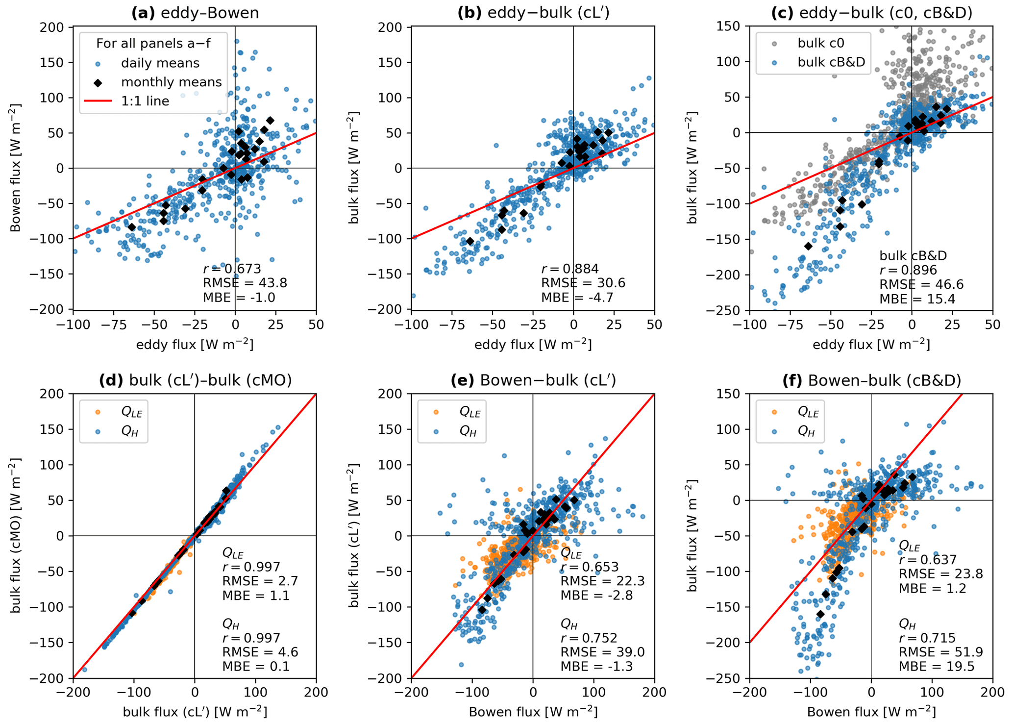
From the comparison of the measured eddy-covariance fluxes and the calculated Bowen and bulk fluxes (daily averages), we reach the following conclusions.

Overall, the modified Louis (1979) parameterisation (cL^′) seems the best choice to parameterise the turbulent fluxes on Murtèl for three reasons. First, as expected, the modified Louis (1979) cL^′ bulk fluxes were near-identical to the iteratively calculated Monin–Obukhov fluxes (Fig. 7d; r=0.996) but at less computational cost. Second, neither filtering nor post-processing was necessary because virtually all estimates met the quality criteria. Third, these show the least deviations from the Bowen fluxes (Fig. 7e), which we consider the benchmark as the Bowen SEB is closed by design. The Bowen fluxes offer reasonable daily estimates based on minimal measurement requirements, namely temperature and specific humidity profiles. Wind speed is not required. The minimum time resolution is daily scale. Hourly values either are numerically unstable (small $\mathrm{\Delta }T/\mathrm{\Delta }q$, especially over a “warm” spring–early-summer snow cover) or do not account for the systematic diurnal wind speed variations. In summer, for example, hourly sensible Bowen fluxes are overestimated during the calm nights and compensated by excessive daytime fluxes.

The eddy-covariance flux systematically underestimates the sensible turbulent flux by a factor of ∼2, leading to a large imbalance (underclosure) in the eddy SEB. The error from the lacking SND correction (Sect. 3.2.2) cannot account for the eddy SEB imbalance. The ratio between the eddy sensible flux and the (sonic) buoyancy flux is between 0.93 and 1.05 (10 % and 90 % quantile, respectively; Eq. 2) on a daily average. Since both the air and the ground surface are most often far from saturation, the eddy sensible flux error due to the lacking high-frequency gas analyser is less than 10 % on 617 out of 692 d (89.2 %) with valid Bowen ratios. Larger deviations occur on the remaining 75 d with $\left|Q_{\mathrm{LE}}\right|>\left|Q_{\mathrm{H}}\right|$ (Bowen ratio within −0.6 and 0.5), typically during snowmelt periods (“warm” saturated snow surface), cloudy and rainy summer days (more frequently in summer 2021 than 2022), or during the first snowfall in autumn. Applying the SND correction showed little added value. Nonetheless, the summertime eddy-covariance fluxes correlate reasonably well with the Bowen sensible turbulent fluxes (Fig. 7a) and the modified Louis (1979) bulk fluxes (Fig. 7b) or the driving temperature gradient (Fig. 11a), and therefore random instrumental or data processing errors represent an unlikely explanation. We hypothesise that some hidden systematic reason causes the flux underestimation and the large eddy SEB imbalance, e.g. secondary circulation (Foken, 2008) of the anabatic afternoon winds.

The empirical Businger–Dyer (cB&D) formulation, developed over flat terrain, overestimates the turbulent fluxes and deviates more strongly for larger negative fluxes (“banana” shape; Fig. 7f), despite extensive filtering. Even the bulk parameterisation without stability correction (c0) outperformed cB&D for the summer fluxes under unstable atmospheric conditions (Fig. 7c). This finding agrees well with Steiner et al. (2018) on the Lirung debris-covered glacier that shares many topo-climatic features with the Murtèl rock glacier (unstable atmosphere over a strongly heated debris surface with anabatic valley winds).

Finally, we describe the relation between the wintertime sensible Bowen fluxes with the driving temperature gradient ΔT (“surface temperature deficit”) as quadratic (Fig. 11b). A quadratic functional Q_H–ΔT relation is unique to the katabatic model of Oerlemans and Grisogono (2002). Note that the Bowen fluxes are independent of wind speed (Eq. 8). Together with the ad hoc “katabatic correction”, our data show that the turbulent fluxes in a snow-covered cirque with katabatic winds might be better parameterised by a katabatic model than by the common Monin–Obukhov bulk method, as also found by Radić et al. (2017) on a sloped glacier surface and discussed by Grisogono et al. (2007) in the context of atmospheric boundary layer modelling.

Figure 11 Comparison of the turbulent sensible flux estimates with the driving temperature difference ΔT (a–c) and atmospheric wind speed u (d–f) motivated by Eq. (12) (daily and monthly averages). Measured winter eddy fluxes are weakly sensitive to local ΔT (a) and u (d). Sensible Bowen flux shows a seasonally differing Q_H–ΔT relation: quasi-linear in summer and quadratic in winter (b) (with best-fit lines). Relation to wind speed u also differs seasonally (e), with a clearer increase in Q_H with wind speed in summer. Note that wind speed is not an input variable for the Bowen parameterisation. The seasonally differing Q_H–ΔT relation reflects the seasonally differing atmospheric stability and wind conditions: stronger dependency on ΔT in the unstable summer atmosphere. The quadratic relation found for the wintertime fluxes suggests that katabatic nocturnal drainage winds govern the turbulent heat transfer (Oerlemans and Grisogono, 2002). Different parameterisations of the bulk fluxes (c) show different sensitivities to ΔT: c0 and cB&D are over-sensitive to ΔT in winter and summer, respectively.

6.3 Micro-scale landform effects on turbulent flux parameters

The “surface” temperature T_s and “surface” specific humidity q_s are key inputs for the Bowen ratio (Eq. 8) and bulk methods to estimate turbulent fluxes (Eqs. 12–13). However, heat and moisture can be drawn from the ventilated AL beneath the surface, provided the snow cover is sufficiently thin to allow convective exchange ($h_{\mathrm{S}}{<}^{\text{SEB}}{\widehat{h}}_{\mathrm{S}}^{\text{crit}}$). Although an “open” snow cover that allows vertical convective exchange between the AL and the atmosphere (Sect. 6.3.1) shapes the wintertime ground thermal regime up to a snow height of ∼70 cm, we will argue in Sect. 6.3.2 and 6.3.3 that already at more than 20 cm of snow convective exchange across the snow cover can be ignored in the context of our SEB.

6.3.1 Snow cover and AL–atmosphere coupling

The snow cover controls the coupling between the coarse blocky AL and the atmosphere. The turbulent fluxes draw heat and moisture from the AL as long as the snow cover is “open” via snow funnels, a phenomenon widely observed on coarse blocky landforms (Sawada et al., 2003; Delaloye et al., 2003; Delaloye and Lambiel, 2005; Morard et al., 2008; Schneider, 2014; Kellerer‐Pirklbauer et al., 2015; Popescu et al., 2017). A thickening snow cover gradually suppresses the vertical convective coupling between the AL and the atmosphere, as more snow funnels close (sketched by the schematic envelopes in Fig. 4). A snow height of ∼10 cm begins to decouple the coarse blocky AL from the atmosphere (“semi-closed” in Fig. 4), but much more snow (∼70 cm) is necessary to achieve the insulating effect of the snow cover on the ground thermal regime (“closed/insulating”). Then, the snow cover is thick enough to suppress convective air exchange, rapid sub-daily fluctuations are strongly attenuated, and large temperature and moisture gradients to the outside air build up (Haberkorn et al., 2015), indicating that the AL–atmosphere coupling is weak. Such a high value is typical for a terrain as rough and blocky as on Murtèl, agreeing with, for example, Hanson and Hoelzle (2004) and Herz (2006). The insulating effect of a thick snow cover was already observed decades ago and used to indirectly map the permafrost distribution using the bottom temperature of snow cover (BTS) method (Haeberli, 1973; Haeberli and Patzelt, 1982).

As regards the SEB, a snow cover as thin as ${}^{\text{SEB}}{\widehat{h}}_{\mathrm{S}}^{\text{crit}}=\mathrm{20}$ cm causes a decoupling that is strong enough for our SEB to be significant. This is shown in the snow-poor winter 2021–2022 with snow depths between 40 and 70 cm, when the ground heat flux Q_G kept fluctuating but remained below the 20 W m⁻² uncertainty threshold (Table 3). The convective flux across the snow cover cannot deviate strongly from Q_G because it was the single largest heat flux to supply/extract the heat for the AL sensible heat storage changes (small conductive snow heat flux, Q_S±2 W m⁻², T_s<0 °C, and no latent effects from snowmelt in that period). We take this threshold as the critical snow thickness (${}^{\text{SEB}}{\widehat{h}}_{\mathrm{S}}^{\text{crit}}$; Eq. 11). We emphasise that the 20 cm threshold is an operational definition for the “decoupled” snow cover in the context of our SEB and its uncertainties.

6.3.2 “Surface” temperature and near-surface ventilation

From Sect. 6.3.1 it follows that for the decoupling or insulating snow cover ($h_{\mathrm{S}}{\ge }^{\text{SEB}}{\widehat{h}}_{\mathrm{S}}^{\text{crit}}$), the reference surface coincides with the snow surface. The radiometric surface temperature represents the surface temperature T_s (Eqs. 8, 12). Whenever the snow cover is open or under snow-free conditions ($h_{\mathrm{S}}{<}^{\text{SEB}}{\widehat{h}}_S^{\text{crit}}$), the radiometric surface temperature is the input meteorological variable T_s (Eq. 12). The surface is where the solar radiation is intercepted and transformed to thermal energy, hence the main source of sensible heat for Q_H. The large gradient $(T_{\mathrm{a}}-T_{\mathrm{s}})/z_{\mathrm{T}}$ drives the sensible turbulent flux Q_H (Eqs. 8, 12; Fig. 12a) and the wind-forced ventilation (Fig. 12b) (Panz, 2008; Stocker-Mittaz, 2002). This is shown by the measured eddy-covariance flux (Fig. 12c) that largely follows the difference between air and radiometric surface temperatures (Fig. 12a, red area), as do the local (anabatic) wind in the atmosphere above the surface and the airflow speed in the near-surface AL (Fig. 12b). During daytime with strong heating on the low-albedo surface, the blocky surface exceeds air temperatures by >15 °C.

However, we found evidence of near-surface ventilation that cannot be parameterised by the 2 m air temperature and the radiometric ground surface temperature: nocturnal Balch ventilation, a nighttime cooling process owed to the interplay of the air permeability, and the thermal inertia (heat retention) of the coarse blocky AL that is most apparent during fair-weather summer days with clear nights. Upwards turbulent heat export is protracted into the evening hours, long after sunset (S^∗; Fig. 12c), as shown by the measured in-cavity airflow speed (WS/3; Fig. 12b) and the eddy-covariance flux (Fig. 12c). Furthermore, the measured eddy-covariance flux remained upwards-directed in the early morning hours, when the terrain surface has radiatively cooled to air temperature T_s≈T_a or even during reversals T_s<T_a in clear-sky nights (that frequently occur in the Engadine: e.g. 24 out of 31 nights in August 2022). The calculated bulk fluxes driven by 2 m air temperature and radiometric ground surface temperature (rGST; red area in Fig. 12a; Eq. 12) are then close to zero (or even downwards) and do not fully capture this nocturnal drawing of heat from the near-surface AL. The large thermal inertia of the rock mass and the protection from long-wave radiative cooling stabilise the sub-surface air temperatures and keep the air in the roof of the ventilated cavity during the nights warmer than that in the atmosphere outside and that on the ground surface (Fig. 12a; $\text{TK1/1}\approx \text{TK6/1}>T_{\mathrm{a}}\approx T_{\mathrm{s}}$ by ∼4 °C). In the nighttime, the locally stably stratified air in the uppermost cavity roof is hence warmer and more unstable than that in the atmosphere (non-local static stability, Stull, 1991). The high permeability of the coarse blocky AL allows this air to escape upwards into the atmosphere or, equivalently, allows the colder outside air to sink into the cavity, thereby exporting heat (Balch ventilation; Balch, 1900; Millar et al., 2014). Panz (2008) describes an occasional nocturnal sub-surface ventilation on Murtèl when T_s<T_a. Also Yao et al. (2014) interpreted nocturnal near-surface ventilation on the debris-covered Koxkar glacier (Xinjiang, China) from eddy-covariance and temperature data.

We assess this uncertainty by using the cavity roof temperature TK1/1 instead of the conventional 2 m air temperature as input T_a for the bulk fluxes (Eq. 12) and compare the nighttime fluxes (when TK1/1 >T_s). Due to the low wind speeds at night, the estimated nocturnal Balch fluxes are small despite the appreciable temperature gradients (10–20 W m⁻²), maximally 10 W m⁻² larger than the “conventional” bulk flux and within our SEB 20 W m⁻² uncertainty (Table 3). Since the short-wave radiative forcing S^∗ and the wind speed covary in phase, the “conventional” radiometric ground surface temperature and 2 m air temperature measurements are sufficiently adequate to parameterise the turbulent fluxes when sub-daily resolution is not required – especially considering that the chosen parameterisation (stability function) shows a much larger effect on the calculated turbulent flux (Fig. 12c; compare cL^′ with cB&D). We reach a conclusion equivalent to that in Sect. 6.3.1 for the critical snow height: the nocturnal convective processes in summer are within the uncertainties of the daily-averaged SEB but might exert an important cooling effect on the sub-surface energy balance.

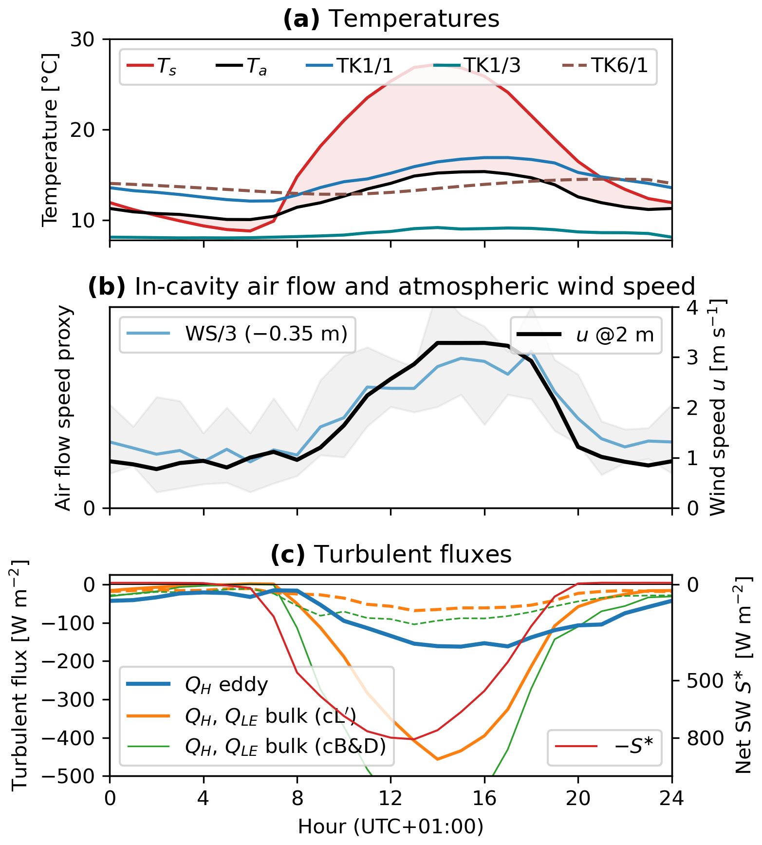
Figure 12 Hourly averages of (a) temperatures, (b) atmospheric wind speed, (c) near-surface AL airflow speed, and (d) sensible turbulent fluxes and net short-wave radiation S^∗ during a summer fair-weather period (15–19 July 2022). The cavity air is stably stratified (TK1/1 > TK1/3), but the air in the cavity roof is warmer and unstable compared with the outside air. During clear summer nights, the atmospheric air and the blocky surface cool down more strongly than the air in the near-surface coarse blocky AL that receives heat from the blocks (air temperature TK1/1 approaches the rock temperature TK6/1 in the night). Conversely to the calculated bulk fluxes, the measured eddy flux decays slowly in the evening–midnight (18–24 h) and remains upwards (negative) despite the small temperature gradient in the early morning (3–7 h, a). The turbulent sensible flux draws heat from the near-surface AL that is nocturnally warmer than T_a and thus unstable. (b, c) Atmospheric wind and AL airflow speeds co-vary in phase (but at ∼ 10× smaller magnitudes), follow the net radiation with some delay, and are closely related to the turbulent fluxes (d). The specific humidity shows small diurnal oscillations; the associated Q_LE varies less than Q_H in absolute terms.

6.3.3 “Surface” humidity and evaporation

From Sect. 6.3.1 it follows that for the decoupling or insulating snow cover ($h_{\mathrm{S}}{\ge }^{\text{SEB}}{\widehat{h}}_{\mathrm{S}}^{\text{crit}}$), the snow surface humidity at saturation $q_{\mathrm{ss}}^{\ast }$ represents the surface specific humidity q_s (Eqs. 8, 13) . Whenever the snow cover is open or under snow-free conditions ($h_{\mathrm{S}}{<}^{\text{SEB}}{\widehat{h}}_{\mathrm{S}}^{\text{crit}}$), the humidity measurement in the cavity roof q_sa is the input meteorological variable q_s (Eq. 11).

Perhaps contrary to the impression of a dry-looking blocky surface, the estimated summertime latent turbulent flux Q_LE is ∼ 30 W m⁻², corresponding to an evaporation rate of ∼ 1 $\mathrm{mm}\mathrm{w}.\mathrm{e}.{\mathrm{d}}^{-\mathrm{1}}$, even during the severe July 2022 dry spell. This value is in the range of evaporation rates reported for debris-covered glaciers of 0.6–2.8 $\mathrm{mm}\mathrm{w}.\mathrm{e}.{\mathrm{d}}^{-\mathrm{1}}$ (Collier et al., 2014; Yao et al., 2014; Steiner et al., 2018). However, note that our evaporative flux estimate Q_LE might be an upper bound, in particular during the July 2022 dry spell. The moisture source for evaporative Q_LE is in the AL, not at the surface (except during precipitation events). However, our bulk parameterisation (C_bt; Eq. 13) ignores the additional resistance to vapour transport imposed by the blocky layer between the specific humidity measurement in the cavity roof and the atmosphere (q_sa is measured 0.7 m beneath the terrain surface; Fig. 2e). The neglected resistance to vapour transport in the coarse blocky AL during moisture-limited evaporation stages, when moisture is drawn from deeper levels and governed by vapour diffusion through the porous AL (Pérez, 1998; Collier et al., 2014), might lead to an overestimation of Q_LE. The longer the dry spell lasts, the deeper in the AL the moisture is drawn from (Sect. 5.2), and the more important this effect of vapour transport resistance becomes. This likely explains why the specific humidity in the cavity roof is almost always (down to sub-hourly timescales) higher than that in the atmosphere despite the relentless mixing by ventilation (moisture surplus relative to the atmosphere; Sect. 5.2), and it possibly accounts for the negative July 2022 SEB imbalance (Fig. 10). The upwards vapour transfer in the comparatively large and strongly ventilated cavity during the dry spell might be overly efficient compared with that in the surrounding AL. This might have led to a non-representatively high specific humidity q_sa in the cavity roof and an overestimated evaporative flux Q_LE.

6.3.4 Aerodynamic roughness lengths

Our mean (median) values of the filtered aerodynamic momentum roughness lengths z_0m of 19 to 7 cm (23–8 cm) agree with the values of Mittaz et al. (2000) and Stocker-Mittaz (2002) of 18 and 7 cm for the snow-free and snow-covered Murtèl surface, respectively (Fig. 9). The scatter range of ∼ 2 orders of magnitude is similar to that in other studies (Brock et al., 2006; Sicart et al., 2014; Radić et al., 2017; Fitzpatrick et al., 2017, 2019). The absolute values are at the upper limit of what has been typically found on debris-covered glaciers (Miles et al., 2017) or on Juvvasshøe by Isaksen et al. (2003) (5 cm), which is plausible given the rough terrain of the Murtèl rock glacier.

The calculated roughness length decreases slightly with increasing snow height by 0.1 cm per cm of snow (Fig. 9b). A similar but much stronger relation between snow height and roughness lengths was found on the Haut Glacier d'Arolla, where Brock et al. (2006) found z_0m to decrease by 2 orders of magnitude with snow heights up to 3 m. This represents a much stronger relation than that on Murtèl, where z_0m decreases by $\sim \mathrm{0.5}\times$ over the observed range of snow thickness. With a maximum snow height of 120 cm (PERMA-XT measurement; Fig. 3) or 200 cm (PERMOS) during the measurement period, the snow cover is thin compared with the terrain roughness (edge length of blocks ∼ 50 cm) and undulations. Both the comparatively high roughness length and the weak sensitivity to snow height might suggest that the aerodynamic roughness is largely controlled by the furrow-and-ridge micro-topography that is not smoothed out by the snow cover or by the few largest blocks that stick out of the snow cover rather than by the average block size. In forests, for comparison, the tallest trees of the canopy have a disproportionally large influence on the aerodynamic roughness (Foken, 2017).

For the bulk parameterisation, we linearly interpolate log ₁₀{z_0m} with snow height. Due to the lack of accurate humidity-corrected sonic temperature measurements, we cannot calculate z_0h or z_0q. We used the unknown ratio ${\widehat{R}}_{z\mathrm{0}}:=z_{\mathrm{0}\mathrm{h}}/z_{\mathrm{0}\mathrm{m}}=z_{\mathrm{0}q}/z_{\mathrm{0}\mathrm{m}}$ as a calibration parameter and found ${\widehat{R}}_{z\mathrm{0}}=\mathrm{2}\times {\mathrm{10}}^{-\mathrm{2}}$. While the approximation z_0h≈z_0q seems applicable, z_0m≈z_0h is not compatible with our parameterisation (Table 3). This agrees with previous studies on debris-covered glaciers (Steiner et al., 2018, 2021) and hummocky ice surfaces (Smeets and van den Broeke, 2008; Sicart et al., 2014).

6.4 Synthesis

The thick coarse blocky AL strongly insulates the underlying permafrost body. We quantified this well-known effect on Murtèl: during the thaw seasons 2021 and 2022, roughly 90 % of the net radiation Q^∗ was exported by the turbulent fluxes and not available to melt ground ice (Fig. 13). The ratio between received surface net radiation Q^∗ to downwards-transmitted heat flux $Q_{\mathrm{r}}=Q_{\mathrm{CGR}\mathrm{3}}^{\mathrm{rad}}$ is $Q^{\ast }:Q_{\mathrm{r}}\approx \mathrm{9}:\mathrm{1}$. This follows from the ratio of the measured in-cavity net long-wave radiation $Q_{\mathrm{CGR}\mathrm{3}}^{\mathrm{rad}}$ to the surface net radiation Q^∗ and the relation $Q_{\mathrm{CGR}\mathrm{3}}^{\mathrm{rad}}=-\mathrm{0.12}{Q}^{\ast }+\mathrm{5.6}$ W m⁻² (R²=0.680). Our measurements corroborate the relation between surface net radiation and ground heat flux that has been found by Hoelzle et al. (2022) using PERMOS data from 1997–2019. Export of the received net radiation is predominantly by sensible fluxes Q_H (50 %–70 %) and secondarily by latent fluxes Q_LE (30 %–50 %; Table 2). Surface albedo (spring–early summer snow cover) and sub-surface thermal and moisture regime of the thick coarse blocky AL control the energy partitioning at/near the surface and the rock glacier's efficiency/ability to export the heat supplied by the surface net radiation Q^∗, the primary heat input (Fig. 5; Table 2).

More heat was transferred into the ground (and more ground ice observed to melt) during the hot and dry summer 2022 than during the cool and wet summer 2021. Two sets of conditions enhanced the downwards heat transfer Q_G in the hot and dry summer 2022 as measured by the sub-surface pyrgeometer, in particular during dry spells and heat waves: first, less snow in winter 2021–2022 and a warm 2022 spring resulted in an early snowmelt in May, 1 month earlier than in summer 2021, and an early start of the thaw season. This exposed the dark low-albedo blocky surface to the strong insolation and the June heat wave, resulting in a rapid rise in ground temperatures and hence an increase in sensible heat storage and downwards ground heat flux (Fig. 8; see Hoelzle et al., 2022, for a 20-year perspective). Second, the 11 d dry spell in July 2022 exhausted the near-surface moisture stores in the coarse blocky AL as indicated by the specific humidity deficit $(q_{\mathrm{sa}}^{\ast }-q_{\mathrm{sa}})$ in the cavity roof (Appendix Fig. B2). Lack of moisture limited the evaporative cooling Q_LE and countered the rock glacier's ability to export the heat (Fig. 8). The moisture storage capacity of the coarse blocky Murtèl AL is limited because the near-surface AL presents a rapid drainage and little fine material (silt) to hold water. During dry spells, the evaporation front recedes quickly to greater depths.

Figure 13 Relation between measured 10 d averaged surface net radiation Q^∗ and measured 10 d averaged in-cavity long-wave radiation $Q_{\mathrm{CGR}\mathrm{3}}^{\mathrm{rad}}$ (of the consecutive 10 d window) summarises the relation between Q^∗, Q_H, and Q_LE. The in-cavity net long-wave radiation $Q_{\mathrm{CGR}\mathrm{3}}^{\mathrm{rad}}$ represents the radiative downward heat transfer Q_r towards the ground ice table (note that upward heat transfer is primarily by convection and not represented by the radiation measurements; $Q_{\mathrm{CGR}\mathrm{3}}^{\mathrm{rad}}=Q_{\mathrm{r}}\approx \mathrm{0}$ W m⁻² during cooling episodes). Of the available net radiation Q^∗, 90 % is exported into the atmosphere by Q_H+Q_LE. Only 10 % is transmitted deeper into the ground and available to warm the AL and to melt ground ice. Latent turbulent heat export is less efficient during dry spells, when the coarse blocky AL dries out and evaporation becomes increasingly moisture-limited (outliers from June, July 2022). The relations between in-cavity long-wave radiation and air temperature, surface temperature ($\propto L^{\uparrow }$), or Q_H are qualitatively similar.

Efficient evaporative cooling relies on frequent precipitation events to resupply, as occurred in summer 2021. With climate change, both factors – early start of the thaw season and hot and dry weather spells in summer – are projected to worsen. A shift to earlier snowmelt and an increase in the number of snow-free days has already been observed in the Swiss Alps (Hoelzle et al., 2022) and is projected to continue with climate change (Scherler et al., 2013; Marmy et al., 2016). Also, the frequency, duration, and intensity of heat waves and dry spells are likely to increase. Changes in the SEB of the thermally conditioned rock glaciers and other mountain permafrost landforms entail changes in the ground thermal regime and ground ice content first and, ultimately, morphological changes: thawing, melting of ground ice, and degradation.

7 Conclusions

We estimated the year-round surface energy balance (SEB) of the seasonally snow-covered ventilated coarse blocky active layer (AL) of the active Murtèl rock glacier that is situated in a cirque in the Upper Engadine (eastern Swiss Alps). The meso-scale landscape produces seasonally contrasting atmospheric conditions of downslope katabatic jets in winter and a strongly unstable atmosphere in summer. At landform scale, the ventilated near-surface AL acts as a buffer layer where heat and moisture transfer is coupled to the atmosphere, unless sealed by a thick snow cover. Based on a novel sensor array located above the ground surface and in the AL that expands an on-site automatic weather station from the Swiss Permafrost Monitoring Network (PERMOS), we were able to improve previous SEB calculations on Murtèl by Mittaz et al. (2000) and Scherler et al. (2014). The measurement period is from September 2020 to September 2022. Our monthly SEB imbalances are within 20 W m⁻² except during the snowmelt months. The main findings concern (i) the climate resilience of the Murtèl rock glacier and (ii) technical aspects of the turbulent flux parameterisations.

• i.

  Two crucial factors for climate resilience of the Murtèl rock glacier are the insulating high-albedo snow cover and a near-complete energy turnover during the snow-free thaw season. The two meteorologically contrasting years studied in this work with the cool and wet summer 2021 and the hot and dry summer 2022 were traced into the SEB and ground thermal and moisture regime. First, an early snowmelt in 2022 prolonged the thaw season, exposed the dark blocky surface to the intense July insolation, and increased AL temperature gradients and the downward heat flux. Second, about 90 % of the received surface net radiation was exported and only 10 % effectively transferred towards the ground ice table and available to melt ground ice. Heat export occurs predominantly via sensible turbulent flux and secondarily via the latent turbulent flux from evaporation. The degree of energy turnover and the turbulent flux partitioning is co-controlled by the availability of moisture for evaporation. Dry spells and heat waves counter the rock glacier's ability to export heat by limiting evaporative fluxes leaving the rapidly drying coarse blocky AL, since the moisture storage capacity is limited. Both trends – earlier snowmelt and more heat waves and dry spells – are projected to continue with climate change. This potentially renders coarse blocky landforms vulnerable to heat waves and dry spells.

• ii.

  With our in-mountain permafrost unprecedentedly comprehensive in situ measurements of eddy-covariance flux, liquid precipitation, snow height, AL temperature and humidity profiles, sub-surface airflow speeds, and sub-surface long-wave radiation, we tested different bulk parameterisations and constrained their input parameters.

  • We parameterised the year-round turbulent fluxes using the modified Louis (1979) scheme (Song, 1998) despite seasonally contrasting atmospheric stability and wind profiles. Wintertime katabatic wind speeds needed to be scaled to close the SEB, which hints at the limits of parameterisations based on the Monin–Obukhov similarity theory in complex mountain terrain and katabatic drainage winds.

  • Sensible and latent partitioning of the turbulent fluxes using the simple Bowen ratio approach agreed with the bulk fluxes on monthly to daily resolution. Given its parsimony and independence from atmospheric stability and wind speed, the Bowen approach represents a valuable and robust tool to estimate the turbulent fluxes in complex terrain with a strongly heterogeneous wind field, provided sub-daily resolution is not required.

  • Since daily oscillations of wind speed and insolation are nearly in phase, the sensible turbulent flux Q_H is driven by the gradient between radiometric ground surface temperature T_s and air temperature T_a. The heat flux Q_H from nocturnal ventilation of the permeable coarse blocky AL is small due to low wind speeds at night. Using a radiometric surface temperature is convenient for modelling Q_H with remotely sensed data.

  • During the thaw season, the evaporative turbulent flux Q_LE is 30 %–50 % of the sensible turbulent flux as a function of moisture availability in the near-surface AL. During dry spells, the near-surface moisture stores are exhausted within days, and moisture supply to the surface is limited by the convective vapour transport from the deeper AL.

  • Measured eddy-covariance fluxes were systematically too small to close the SEB. Still, the eddy-derived momentum roughness length z_0m corroborates previous aerodynamic estimates from Mittaz et al. (2000). z_0m varies seasonally between 7 and 20 cm as a function of snow height that smooths the landscape.

Appendix A: Turbulent flux parameterisations

Different formulations of the stability functions exist. Here, we compare the widely used Businger–Dyer relations with the formulation from Louis (1979) and the iterative Monin–Obukhov scheme.

A1 Businger and Dyer parameterisation

In the Businger and Dyer parameterisation (denoted by “cB&D”), the bulk transfer coefficient C_bt is expressed as

$$\begin{array}{}\text{(A1)}& C_{\mathrm{bt}}={\displaystyle \frac{k_{\ast }^{\mathrm{2}}}{\ln \left\{\frac{z_{\mathrm{u}}}{z_{\mathrm{0}\mathrm{m}}}\right\}\ln \left\{\frac{z_{T/q}}{z_{\mathrm{0}h/q}}\right\}}}({\mathit{\varphi }}_{\mathrm{m}}{\mathit{\varphi }}_{h/q}{)}^{-\mathrm{1}},\end{array}$$

where the Businger–Dyer non-dimensional stability functions for heat and water vapour are expressed as a function of the bulk Richardson number Ri_b (Eq. A3) (Brutsaert, 1982; Oke, 1987),

$$\begin{array}{}\text{(A2)}& \begin{array}{rl}({\mathit{\varphi }}_{\mathrm{m}}{\mathit{\varphi }}_{\mathrm{h}}{)}^{-\mathrm{1}}& =({\mathit{\varphi }}_{\mathrm{m}}{\mathit{\varphi }}_q{)}^{-\mathrm{1}}\\ & =\left\{\begin{array}{ll}(\mathrm{1}-\mathrm{5}{\mathit{Ri}}_{\mathrm{b}}{)}^{\mathrm{2}},& \text{for}\mathrm{0.0}\le {\mathit{Ri}}_{\mathrm{b}}\le \mathrm{0.2}\text{(stable case)}\\ (\mathrm{1}-\mathrm{16}{\mathit{Ri}}_{\mathrm{b}}{)}^{\mathrm{0.75}},& \text{for}{\mathit{Ri}}_{\mathrm{b}}<\mathrm{0.0}\text{(unstable case)}\end{array}\right.\end{array}\end{array}$$

that corrects for non-neutral stability of the near-surface atmosphere (atmospheric stratification). These are unity in the case of neutrally stable atmosphere (Ri_b=0), denoted by “c0”. Used constants and parameters are the von Kármán constant k_∗ (0.40); the roughness lengths for momentum z_0m, heat z_0h, and water vapour z_0q; and the (constant) measurement heights for wind speed z_u [m], temperature z_T, and humidity z_q above the ground surface. In this work, the variable sensor height above the snow surface is accounted for by correcting the wind speed u rather than simply subtracting the snow height from the sensor distance above the ground for site-specific reasons discussed in Sect. 6.2.

The Businger–Dyer and the modified Louis (1979) parameterisations characterise atmospheric stability with the bulk Richardson number Ri_b defined by

$$\begin{array}{}\text{(A3)}& {\mathit{Ri}}_{\mathrm{b}}:={\displaystyle \frac{g}{\stackrel{\mathrm{‾}}{T}}}{\displaystyle \frac{\frac{T_{\mathrm{a}}-T_{\mathrm{s}}}{z_{\mathrm{T}}-z_{\mathrm{0}\mathrm{h}}}}{{\left(\frac{u}{z_{\mathrm{u}}-z_{\mathrm{0}\mathrm{m}}}\right)}^{\mathrm{2}}}},\end{array}$$

with the average temperature $\stackrel{\mathrm{‾}}{T}:=(T_{\mathrm{a}}+T_{\mathrm{s}})/\mathrm{2}$ [K].

However, this widely used stability function (Reid and Brock, 2010; Brock et al., 2010; Mittaz et al., 2000; Favier et al., 2004; Steiner et al., 2018; Scherler et al., 2014) yields implausible fluxes when the atmosphere strongly deviates from near-neutral stability conditions, $\left|{\mathit{Ri}}_{\mathrm{b}}\right|>\mathrm{0.2}$. Equation (A2) is invalid for ${\mathit{Ri}}_{\mathrm{b}}>+\mathrm{0.2}$ and tends to diverge for highly unstable atmospheres at low wind speeds where ${\mathit{Ri}}_{\mathrm{b}}\to -\mathrm{\infty }$. Filtering out these fluxes as proposed by Steiner et al. (2018) potentially deletes a sizeable portion of the calculated fluxes at the wind-sheltered Murtèl cirque.

A2 Modified Louis (1979) scheme

The Louis (1979) scheme is an analytical approximation of the iterative Monin–Obukhov scheme. The bulk exchange factor is expressed as C_bt=f_hC_Hn (notation from Essery and Etchevers, 2004), where $C_{\mathrm{Hn}}=k_{\ast }^{\mathrm{2}}\ln \mathit{\{}{z}_{\mathrm{u}}/z_{\mathrm{0}}{\mathit{\}}}^{-\mathrm{2}}$ (the neutral exchange coefficient) and

$$\begin{array}{}\text{(A4)}& f_{\mathrm{h}}=\left\{\begin{array}{ll}(\mathrm{1}+\mathrm{10}{\mathit{Ri}}_{\mathrm{b}}{)}^{-\mathrm{1}},& \text{for}{\mathit{Ri}}_{\mathrm{b}}\ge \mathrm{0}\text{(stable case)}\\ \mathrm{1}-\mathrm{10}{\mathit{Ri}}_{\mathrm{b}}(\mathrm{1}+\mathrm{10}{C}_{\mathrm{Hn}}\sqrt{-{\mathit{Ri}}_{\mathrm{b}}}/f_z{)}^{-\mathrm{1}},& \text{for}{\mathit{Ri}}_{\mathrm{b}}<\mathrm{0}\text{(unstable case)}\end{array}\right.\end{array}$$

with

$$\begin{array}{}\text{(A5)}& f_z={\displaystyle \frac{\mathrm{1}}{\mathrm{4}}}\sqrt{{\displaystyle \frac{z_{\mathrm{0}}}{z_{\mathrm{u}}}}}.\end{array}$$

However, one shortcoming of the Louis (1979) scheme critical on rough surfaces is the assumption of equal momentum roughness length (z_0m) and sensible heat roughness length (z_0h), i.e. $z_{\mathrm{0}\mathrm{m}}=z_{\mathrm{0}\mathrm{h}}=z_{\mathrm{0}}$. Hence, we use the Louis (1979) scheme modified by Song (1998) (denoted by “cL^′”). The implementation is described in Rigon et al. (2006) and Endrizzi et al. (2014).

A3 Iterative Monin–Obukhov scheme

In the Monin–Obukhov scheme (denoted by “cMO”), the atmospheric stability is characterised by the Obukhov length L defined by

$$\begin{array}{}\text{(A6)}& L={\displaystyle \frac{u_{\ast }^{\mathrm{3}}}{k_{\ast }\frac{g}{T_{\mathrm{a}}}\frac{Q_{\mathrm{H}}}{{\mathit{\rho }}_{\mathrm{a}}{C}_p}}},\end{array}$$

where u_∗ [m s⁻¹] is the friction velocity. The bulk exchange factor for heat C_bt=C_MO is given by (Conway and Cullen, 2013; Fitzpatrick et al., 2017; Steiner et al., 2018)

$$\begin{array}{}\text{(A7)}& C_{\mathrm{MO}}={\displaystyle \frac{k_{\ast }^{\mathrm{2}}}{\left[\ln \left\{\frac{z_{\mathrm{u}}}{z_{\mathrm{0}\mathrm{m}}}\right\}-{\mathit{\psi }}_{\mathrm{m}}\left(\frac{z_{\mathrm{u}}}{L}\right)+{\mathit{\psi }}_{\mathrm{m}}\left(\frac{z_{\mathrm{0}\mathrm{m}}}{L}\right)\right]\left[\ln \left\{\frac{z_{\mathrm{T}}}{z_{\mathrm{0}\mathrm{h}}}\right\}-{\mathit{\psi }}_{\mathrm{h}}\left(\frac{z_{\mathrm{T}}}{L}\right)+{\mathit{\psi }}_{\mathrm{h}}\left(\frac{z_{\mathrm{0}\mathrm{h}}}{L}\right)\right]}},\end{array}$$

where ψ_m and ψ_h are the vertically integrated stability functions for momentum and heat, respectively. The latent flux Q_LE is calculated analogously to scalar roughness length for water vapour z_0q and the integrated stability function for water vapour ψ_q, both assumed equal to the corresponding quantity and function for heat. Since L depends itself on Q_H, C_MO is calculated iteratively.

Different formulations are available for the integrated stability function ψ as used by, for example, Fitzpatrick et al. (2017), Steiner et al. (2018), and Sauter et al. (2020). We use the following momentum ψ_m and heat ψ_h stability functions (again assuming ψ_h=ψ_q) (Fitzpatrick et al., 2017):

$$\begin{array}{}\text{(A8)}& \begin{array}{rl}& {\mathit{\psi }}_{\mathrm{m}}\left(\mathit{\zeta }\right)\\ & =\left\{\begin{array}{ll}-\left[a\mathit{\zeta }+b\left(\mathit{\zeta }-\frac{c}{d}\right)\exp \left\{-d\mathit{\zeta }\right\}+\frac{bc}{d}\right],& \mathit{\zeta }>\mathrm{1}\\ & \text{(stable (Beljaars and Holtslag, 1991))}\\ \ln \left\{\left(\frac{\mathrm{1}+{\mathit{\chi }}^{\mathrm{2}}}{\mathrm{2}}\right){\left(\frac{\mathrm{1}+\mathit{\chi }}{\mathrm{2}}\right)}^{\mathrm{2}}\right\}\\ -\mathrm{2}\arctan \mathit{\chi }+\frac{\mathit{\pi }}{\mathrm{2}},& \mathit{\zeta }<\mathrm{0}\\ & \text{(unstable (Dyer, 1974))}\end{array}\right.\end{array}\end{array}$$

and the heat stability function ψ_h

$$\begin{array}{}\text{(A9)}& \begin{array}{rl}& {\mathit{\psi }}_{\mathrm{h}}\left(\mathit{\zeta }\right)\\ & =\left\{\begin{array}{l}-\left[{\left(\mathrm{1}+\frac{\mathrm{2}a}{\mathrm{3}}\mathit{\zeta }\right)}^{\mathrm{1.5}}\right.\\ \left.+b\left(\mathit{\zeta }-\frac{c}{d}\right)\exp \left\{-d\mathit{\zeta }\right\}+\frac{bc}{d}-\mathrm{1}\right],& \mathit{\zeta }>\mathrm{1}\\ & \text{(stable (Beljaars and Holtslag, 1991))}\\ \mathrm{2}\ln \left(\frac{\mathrm{1}+{\mathit{\chi }}^{\mathrm{2}}}{\mathrm{2}}\right),& \mathit{\zeta }<\mathrm{0}\\ & \text{(unstable (Dyer, 1974))}\end{array}\right.\end{array}\end{array}$$

with the dimensionless Obukhov parameter $\mathit{\zeta }:=z_{\mathrm{u}}/L$ (for ψ_m) or $z_{\mathrm{T}}/L$ (for ψ_h), $\mathit{\chi }=(\mathrm{1}-\mathrm{16}\mathit{\zeta }{)}^{\mathrm{1}/\mathrm{4}}$, a=1, $b=\mathrm{2}/\mathrm{3}$, c=5, and d=0.35.

Appendix B: Ground thermal and hygric regimes

The ground thermal and hygric regimes are shown in Figs. B1 and B2. These are the meteorological input variables for the calculation of the turbulent fluxes.

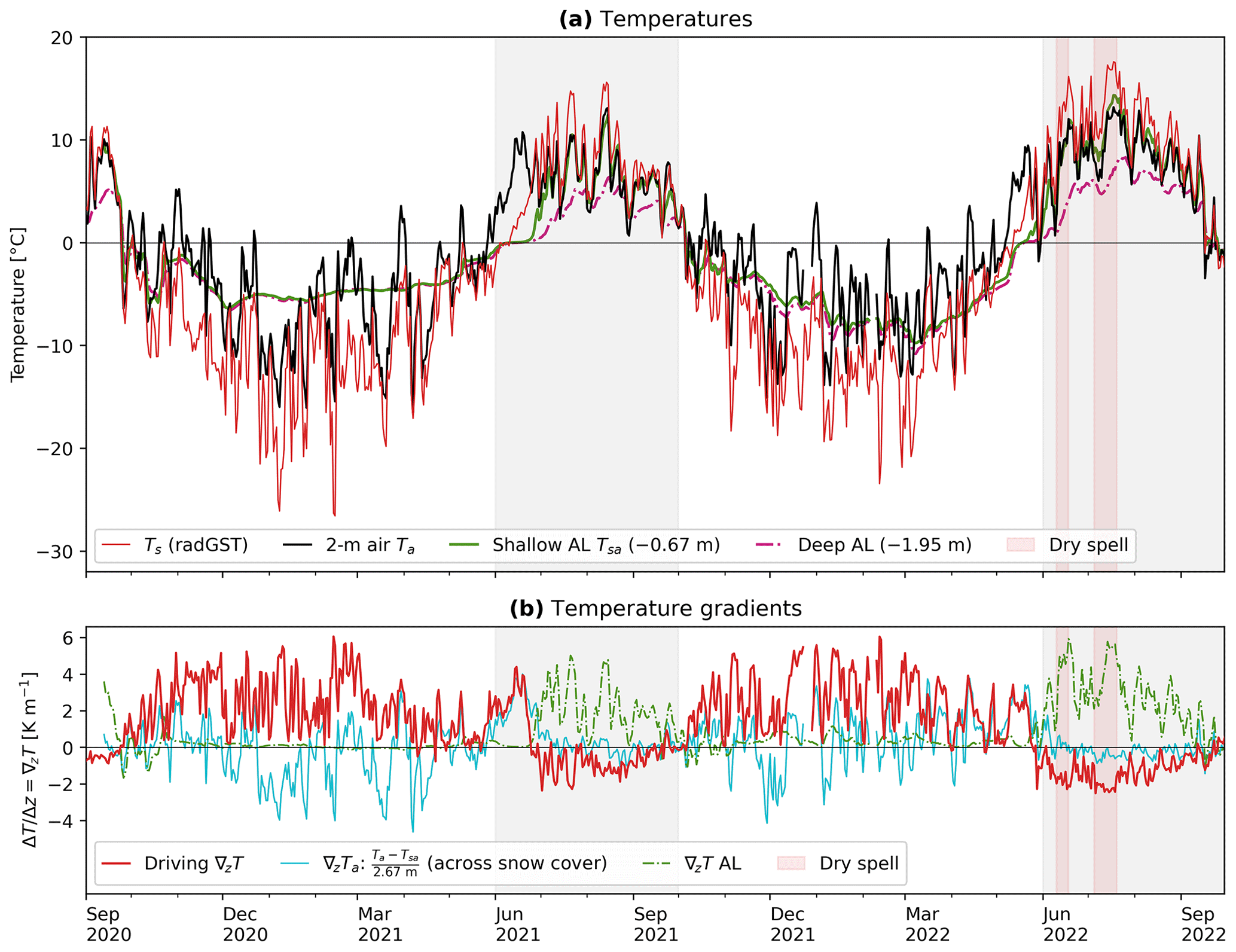
Figure B1 Thermal regime. (a) Radiometric ground surface temperature T_s (“rGST”) and air temperatures in the atmosphere T_a and in the instrumented cavity (cavity roof T_sa at 0.67 m and mid-cavity level at 1.95 m depth). (b) Vertical temperature gradients ∇_zT between surface and 2 m air temperature (drives turbulent sensible fluxes; Eq. 12), across the snow cover (T_a−T_sa), and within the cavity (indicates the stability of the in-cavity air column). The summer 2022 dry spells are referred to in the text.

Figure B2 Hygric regime. (a) Relative and specific humidity of the saturated snow surface $q_{\mathrm{ss}}^{\ast }$, in the atmosphere q_a, and in the instrumented cavity (q_sa cavity roof at 0.67 m and mid-cavity level at 1.95 m depth). (b) Vertical specific humidity gradients (∇_zq) between the atmospheric air and the surface (either $q_{\mathrm{ss}}^{\ast }$ or q_sa according to Eq. 11), across the snow cover (q_a−q_sa), and within the cavity (indicates the moisture transport direction). The moisture transport within the cavity is generally downwards (∇_zq>0), and condensation rather than evaporation occurs in the deep AL. Severe dry spells that last long enough to exhaust the near-surface moisture storage (∼ 5 d) strongly impact the ground moisture regime, reverse the moisture gradients, and lead to upwards moisture transport.

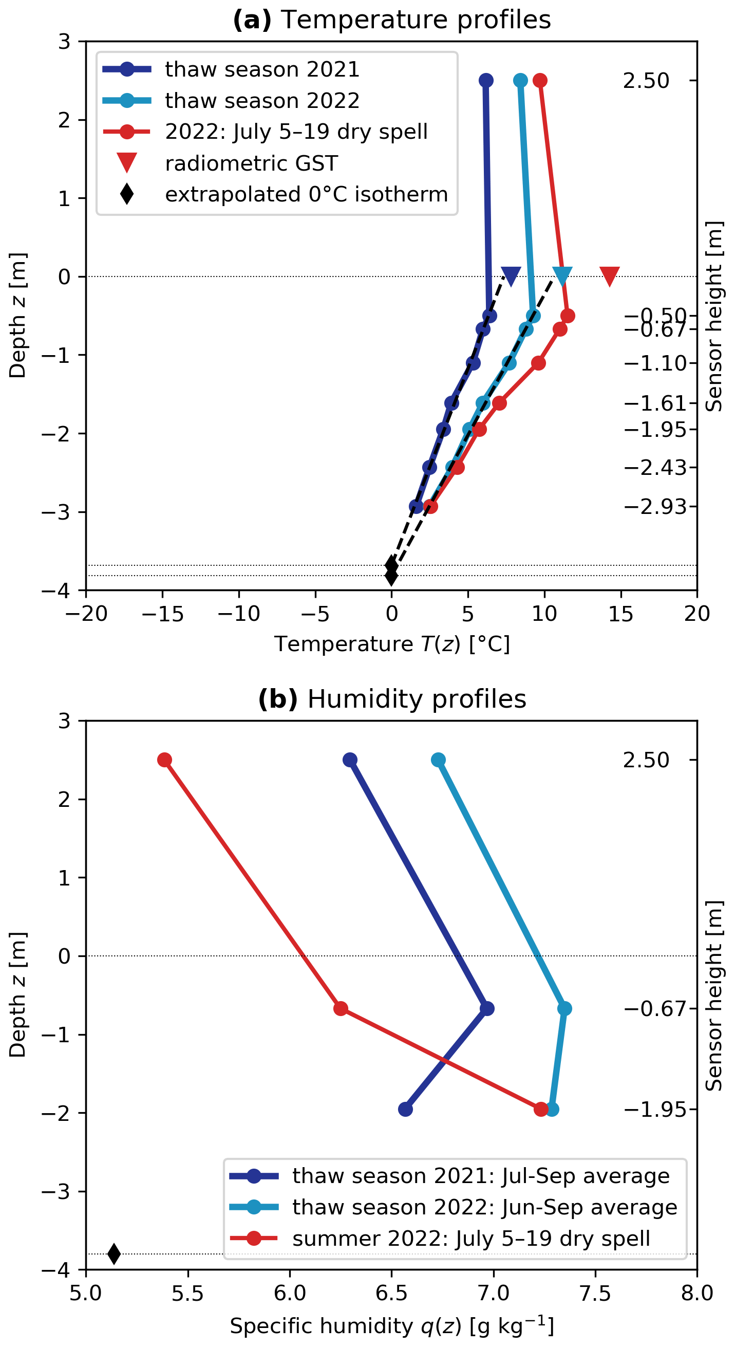
Figure B3 (a) Vertical temperature and (b) specific humidity profile (thaw-season average). Temperature and humidity are highest in the near-surface AL. The near-surface AL in contact with the atmosphere responds to dry spells and dries out within a few days after the last precipitation event. The deep AL remains close to saturation.

Appendix C: Estimate of the thermal relaxation time

An estimate for the thermal relaxation time Δt_r of a packed bed is

$$\begin{array}{}\text{(C1)}& \mathrm{\Delta }{t}_{\mathrm{r}}\approx {\displaystyle \frac{{\mathit{\rho }}_{\mathrm{r}}{c}_{\mathrm{r}}}{h_{\text{eff}}}}{\displaystyle \frac{V}{A_s}}={\displaystyle \frac{{\mathit{\rho }}_{\mathrm{r}}{c}_{\mathrm{r}}}{h_{\text{eff}}}}{\displaystyle \frac{(d_{\mathrm{p}}/\mathrm{2})}{\mathrm{3}(\mathrm{1}-{\mathit{\varphi }}_{\mathrm{al}})}},\end{array}$$

where h_eff is the effective heat transfer coefficient calculated via $\mathrm{1}/h_{\text{eff}}=\mathrm{1}/h+d_{\mathrm{p}}/\left(\mathrm{10}{k}_{\mathrm{r}}\right)$ (Esence et al., 2017). This correction accounts for the additional resistance arising from the temperature gradients within large blocks. “Large” means blocks whose Biot number exceeds 0.1 (Esence et al., 2017), with the Biot number defined by

$$\begin{array}{}\text{(C2)}& \mathit{Bi}:={\displaystyle \frac{h}{k_{\mathrm{r}}}}L.\end{array}$$

The characteristic length L is given by the ratio of the block volume to surface area: $L:=V/A_s=d_{\mathrm{p}}/\mathrm{6}$ for spheres. A minimum value for the convective heat transfer coefficient h under forced convection at low wind speed (u<1 m s⁻¹) is ∼ 10 $\mathrm{W}{\mathrm{m}}^{-\mathrm{2}}{\mathrm{K}}^{-\mathrm{1}}$. The value is derived from inverting Eq. (12) with $h:=Q_{\mathrm{H}}/(T_{\mathrm{a}}-T_{\mathrm{s}})$ (nighttime values) and agrees with an estimate in Bozhinskiy et al. (1986). With a thermal conductivity of the rock of k_r=2.5 $\mathrm{W}{\mathrm{m}}^{-\mathrm{1}}{\mathrm{K}}^{-\mathrm{1}}$, the critical diameter is 0.15 m. With d_p=60 cm (typical dimension of the blocks enclosing the instrumented cavity), Eq. (C1) yields an estimate of $\mathrm{\Delta }{t}_{\mathrm{r}}=\sim \mathrm{12}$ h. Thermal adjustment (within >95 %) is attained after 3Δt_r or ∼1.5 d for large blocks with 60 cm edge length. Smaller blocks reach thermal equilibrium much faster, e.g. 20 cm blocks within 10 h.

Appendix D: 1997–2000 wind speed profiles

Here, we justify our “katabatic correction” of wind speed measurements with wind profile data collected by Stocker-Mittaz et al. (2002) and Stocker-Mittaz (2002). A 10 m tower installed on the Murtèl rock glacier at the PERMOS monitoring site measured the wind velocity, air temperature, and relative humidity at 1.5, 2.0, 6.5, and 9.1 m a.g.l. between January 1997 and March 2000.

Average vertical wind speed profiles (Fig. D1a) show the winter-time low-level jet between December and March with maximum wind speeds close to the snow-covered surface and upwards decreasing wind speed. In summer, wind speeds increase with height and approximately show the log wind profile (Stocker-Mittaz, 2002). The wind speed gradient is predominantly negative for more than ∼ 75 cm of snow measured at the PERMOS station (located on a plateau) (Fig. D1b), corresponding to ∼ 50 cm at the PERMA-XT station (located on a more wind-swept ridge). This finding justifies the compensation for snow height (Eq. 23) and possibly explains why the “katabatic correction” has less effect on the SEB of the snow-poor winter 2021–2022 and a negative effect on the November 2020 SEB (Fig. 10).

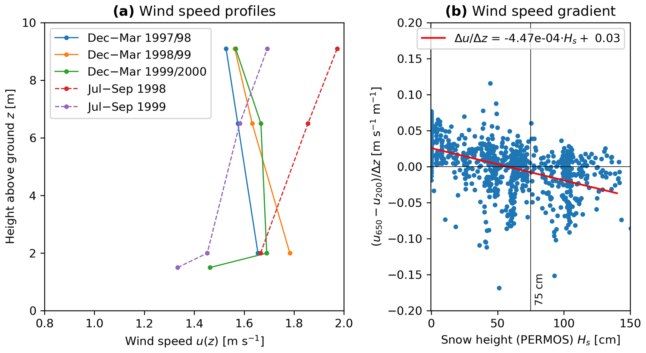
Figure D1 (a) Wind speed profiles for winter (December–March average) and summer (July–September) 1997–2000 (Stocker-Mittaz et al., 2002). Winter storms where wind speed at 9.1 m exceeded 2.5 m s⁻¹ are filtered out (threshold from Stocker-Mittaz, 2002). (b) The average wind speed gradient between the 2.0 and 6.5 m levels switches from a (dominantly) positive log wind profile to a negative low-level jet profile at a (PERMOS) snow height of ∼ 60 cm (R²=0.271). Own figure based on data from Stocker-Mittaz et al. (2002).

Appendix E: Nomenclature

Parameters and constants used in this study are tabulated in Table E1.

Table E1 Nomenclature: measurement variables, site-specific calibration parameters, dimensionless numbers, and constants.