Using Icepack to reproduce ice mass balance buoy observations in landfast ice: improvements from the mushy-layer thermodynamics

Icepack (v1.1.0) – the column thermodynamics model of the Community Ice CodE (CICE) version 6 – is used to assess how changing the thermodynamics from the Bitz and Lipscomb (1999) physics (hereafter BL99) to the mushy-layer physics impacts the model performance in reproducing in situ landfast ice observations from two ice mass balance (IMB) buoys co-deployed in the landfast ice close to Nain (Labrador) in February 2017. To this end, a new automated surface retrieval algorithm is used to determine the in situ ice thickness, snow depth, basal ice congelation and snow-ice formation from the measured vertical temperature profiles. Icepack simulations are run to reproduce these observations using each thermodynamics scheme, with a particular interest in how the different physics influence the representation of snow-ice formation and ice congelation. Results show that the BL99 parameterization represents well the ice congelation but underrepresents the snow-ice contribution to the ice mass balance. In particular, defining snow-ice formation based on the hydrostatic balance alone does not reproduce the negative freeboards observed for several days in the IMB observations, resulting in an earlier snow-flooding onset, a positive ice thickness bias and reduced snow depth variations. We find that the mushy-layer thermodynamics with default parameters significantly degrades the model performance, overestimating both the congelation growth and snow-ice formation. The simulated thermodynamics response to flooding, however, better represents the observations, and the best results are obtained when allowing for negative freeboards in the mushy-layer physics. We find that the mushy-layer thermodynamics produces a larger variability in congelation rates at the ice bottom interface, alternating between periods of exceedingly fast growth and periods of unrealistic basal melt. This pattern is related to persistent brine dilution in the lowest ice layer by the congelation and brine drainage parameterizations. We also show that the mushy-layer congelation parameterization produces significant frazil formation, which is not expected in a landfast ice context. This behavior is attributed to the congelation parameterization not fully accounting for the conductive heat flux imbalance at the ice–ocean boundary. We propose a modification of the mushy-layer congelation scheme that largely reduces the frazil formation and allows for better tuning of the congelation rates to match the observations. Our results demonstrate that the mushy-layer physics and its parameters can be tuned to closely match the in situ observations, although more observations are needed to better constrain them.

1 Introduction

The sea ice and oceanography of the Canadian Arctic are largely modulated by the formation of landfast ice in fjords, along the coasts and in narrow channels. Each winter, this landlocked sea ice transforms the Canadian Arctic Archipelago (CAA) into a seasonal continent of stationary sea ice (Melling, 2002; Galley et al., 2012), effectively insulating the seawater from the cold atmosphere and barring the transport of ice through the CAA passages (Howell et al., 2013; Kwok, 2006). The landfast ice edge represents a seasonal boundary where the air–ocean exchanges and ice dynamics processes are concentrated, in particular by the opening of semipermanent polynyi under divergent surface forcing conditions (Melling et al., 2001; Dumont et al., 2010). These flaw polynyi in turn drive the regional meteorology (Barber et al., 2001; Gultepe et al., 2003; Lüpkes et al., 2008; Raddatz et al., 2011) and ocean circulation (Dumont et al., 2010), producing sediment-rich waters that are key to the Arctic marine ecosystem (Stirling, 1980, 1997; Carmack and Macdonald, 2002; Tremblay et al., 2002). As changes in the landfast ice cover are expected to alter these processes, its monitoring, representation in forecast models and inclusion in climate projections are a concern not only for the study of the Arctic climate but also for a wide range of socio-economical aspects such as on-ice transport safety, food security and navigation planning (Gearheard et al., 2006; Eicken et al., 2011; Cooley et al., 2020).

In dynamic sea ice models, the physics of landfast ice is represented using a combination of thermodynamic relations governing the ice growth and melt (i.e., a column thermodynamics model; Maykut and Untersteiner, 1971; Semtner, 1976; Bitz and Lipscomb, 1999; Huwald et al., 2005; Turner et al., 2013) and of dynamic parameterizations governing its stability against external forces (i.e., a rheological model; Hibler, 1979; Hunke and Dukowicz, 1997; Tremblay and Mysak, 1997; Wilchinsky and Feltham, 2004; Rampal et al., 2016). While these components are mostly treated (and developed) independently, they remain deeply interconnected and the formation of landfast ice usually results from their combined action. In many areas, for instance, the landfast ice is held by the grounding of ice keels on the ocean floor, which involves prior ridging (dynamics) of sufficiently thick ice (thermodynamics). In the absence of ice grounding, landfast ice can form during periods of calm and cold weather (Divine et al., 2004; Kirillov et al., 2021), during which leads freeze to a sufficient ice thickness for the unconsolidated ice floes to coalesce together (thermodynamics), allowing the formation of ice arches between pining points that resist subsequent surface forcings (dynamics;  Dammann et al., 2019; Liu et al., 2022). In sea ice models, this interplay between thermodynamic and dynamic factors is represented by ice thickness dependencies in the dynamic parameters, such as the seabed stress term (Lemieux et al., 2015) or the material strength parameters (Dumont et al., 2009; Lemieux et al., 2016; Plante et al., 2020; Liu et al., 2022). The accurate representation of landfast ice extent, trends and variability in sea ice models therefore requires not only the permitting dynamics (i.e., ice grounding and tensile strength) but also thermodynamics that reproduce well the landfast ice growth and melt.

In the Environment and Climate Change Canada (ECCC) ice–ocean forecasting systems (e.g., RIOPSv2; Smith et al., 2021), the implementation of the aforementioned landfast ice dynamics was shown to greatly improve the representation of landfast ice in hindcast (free-run) simulations (Lemieux et al., 2016). The timings of landfast ice formation and breakup, however, remain difficult to reproduce, often offset by a couple of weeks with respect to those recorded in operation ice charts (Lemieux et al., 2016). While this could be improved by modifications to the ice grounding mechanics (e.g., Dupont et al., 2022) or by changes to the ice strength formulation (Ungermann et al., 2017), it is also possible that the discrepancy is associated with a misrepresentation of the landfast ice thermodynamics, which in the ECCC systems is based on the model of Bitz and Lipscomb (1999) (hereafter BL99). Thermodynamics models have grown in sophistication over the years, in particular with the representation of mushy-layer physics (Feltham et al., 2006), brine dynamics (Notz and Worster, 2009; Turner et al., 2013) and melt ponds (Flocco et al., 2010; Holland et al., 2012; Hunke et al., 2013). These developments are implemented in the Los Alamos Community Ice CodE version 5 (CICE5) and were shown to have competing effects on the overall pan-Arctic ice mass balance, both in long-term global simulations (Turner and Hunke, 2015) and in coupled climate simulations (Community Earth System Model version 2;  Bailey et al., 2020; DuVivier et al., 2021). The use of the mushy-layer physics was in particular shown to produce larger amounts of frazil and snow ice, together increasing the overall ice thickness. Whether this increase is also seen in the landfast ice context (without sensitivities to the offshore sea ice dynamics) remains to be determined.

In recent years, the deployment of ice mass balance (hereafter IMB but used here as a general term not referring to specific designs) buoys in both the Arctic and Antarctic provided in situ observations of the thermodynamics in the sea ice interior by measuring the internal sea ice temperature at a high vertical (cm) and temporal (h) resolution (Richter-Menge et al., 2006; Jackson et al., 2013; Planck et al., 2019). The snow depth and ice thickness conditions are inferred from the recorded vertical temperature profiles, traditionally by visual inspection (Tian et al., 2017; Provost et al., 2017) but more recently by using automated algorithms (Liao et al., 2019; Cheng et al., 2020; Richter et al., 2023). These measurements give new insights into thermodynamic processes that are otherwise not detectable by traditional ice thickness measurements, ice core analyses or remote sensing, such as snow-ice formation (Provost et al., 2017; Rösel et al., 2018), heat fluxes within and between the material interfaces (Trodahl et al., 2000; West et al., 2020), brine convection, and mushy-layer properties (Wongpan et al., 2018). IMB buoys have also been used to assess the performance of thermodynamics models in the context of 1D simulations (Caixin et al., 2015; Tian et al., 2017; Duarte et al., 2020). The mushy-layer physics in CICE version 5, for instance, has been tested against IMBs deployed in the pack ice (first year and multiyear) during the N-ICE2015 expedition north of Svalbard, where it was shown to adequately represent the observed sea ice growth but also to overrepresent snow flooding under large snow depth conditions (Duarte et al., 2020).

In this study, we investigate how updating the model thermodynamics from the BL99 physics to the mushy-layer parameterization impacts the simulated sea ice mass balance in a landfast ice context, away from the pack ice dynamics. This assessment is based on the in situ observations from two IMB buoys that were deployed in a landfast ice channel well sheltered from offshore dynamics, close to Nain (Nunatsiavut, Labrador). A particular interest is placed on the ice growth from congelation and snow-ice formation, which is determined from the recorded internal temperature profiles using a novel surface retrieval algorithm building on the work of Liao et al. (2019) and Cheng et al. (2020). Multiple Icepack (v1.1.0) model simulations (Hunke et al., 2023) are run to reproduce these observations using the BL99 physics or the mushy-layer physics to determine the effect of the brine physics on the model's performance. In particular, we find that the use of the mushy-layer physics with default parameters significantly degrades the model performance despite the improved representation of flooding and brine processes. The basal ice growth in mushy simulations is overrepresented, includes a significant contribution from frazil production and exhibits unexpected periods of basal melt. The snow-ice formation is also overrepresented due to early snow flooding when observations are under negative freeboard conditions. We show that these discrepancies are largely resolved by simple modifications and tunings of the congelation and snow-ice parameterizations. The contributions of this paper include a modified mushy-layer congelation parameterization not conducive to frazil formation and a parameterized dependency of the snow flooding rate on negative freeboard values.

This paper is organized as follows. A description of the buoys and surface forcing data used in the analysis is provided in Sect. 2. The Icepack model physics are briefly presented in Sect. 3, first describing the BL99 physics currently used in the ECCC forecast systems and then the differences when using the mushy-layer thermodynamics. Our modifications to the congelation and snow-ice parameterizations are also included in Sect. 3. The methods are detailed in Sect. 4, including the surface retrieval algorithm, the numerical simulation setup and the model performance diagnostics. Results from the in situ observations and Icepackv1.1.0 simulations are presented in Sect. 5. Discussions of the model performance and conclusions are summarized in Sect. 6.

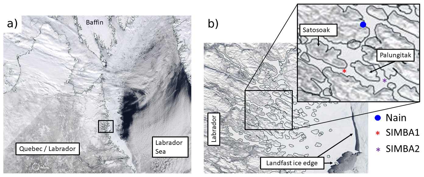
Figure 1 Location of the two snow ice mass balance apparatus (SIMBA) buoys on the Labrador coast (a) and in a landfast ice channel close to the Nain community (b). The buoys are located at ∼56.42° N, 61.7° W (SIMBA1) and ∼56.43° N, 61.50° W (SIMBA2), ∼ 12 km from each other and ∼50 km from the nearest landfast ice edge. Images are corrected reflectance imagery taken from MODIS Worldview (https://earthdata.nasa.gov/labs/worldview/, last access: 7 September 2023).

2 Data

2.1 Ice mass balance buoy observations

Two Scottish Association for Marine Science (SAMS) snow ice mass balance apparatus (hereafter SIMBA) buoys were deployed in winter 2017 as part of an ongoing collaboration with the Nunatsiavut Research Centre (NRC), with the goal of serving the Nain community with the deployment of scientific instruments in the local landfast ice. The buoys were thus not deployed as part of a wider scientific field observation campaign: the deployment dates and locations were chosen with NRC collaborators based on their sea ice monitoring interests. The first buoy (SIMBA1) was deployed on 23 February 2017 at ∼56.42° N, 61.7° W in a landfast channel close to the southern coast of Satosoak Island (see Fig. 1) and recovered 2 months later on 18 April. The second buoy (SIMBA2) was deployed during the same season on 24 February at ∼56.43° N, 61.50° W, ∼12 km east of SIMBA1 in the same fjord close to Palungitak Island and recovered 3 months later on 31 May. To our knowledge, this was the first time IMB buoys were deployed in this area.

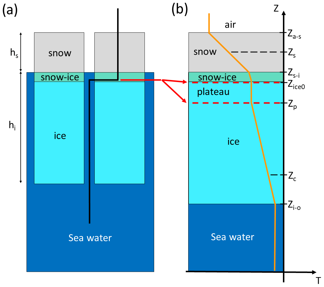
Figure 2 Schematics of the deployed SIMBA buoy thermistor strings through the snow, snow-ice and sea ice layers (a) and the vertical temperature profiles they measure, with the sensor positions identified by the surface retrieval algorithm (b). Note the section of the thermistor string (thermistor plateau, red lines) laid flat on the bare ice surface at deployment but later embedded within the ice layer after flooding. The marked sensor locations are, from top to bottom as follows: the air–snow interface (Z_a−s), the snow interior (Z_s), the snow–ice interface above the snow ice (Z_s−i), the snow–ice interface at deployment (Z_ice0), the lower end of the thermistor plateau (Z_p), a point in the ice interior close to the ice–ocean interface (Z_c) and the ice–ocean interface (Z_i−o).

The SIMBA buoys consist of a 5 m long thermistor string with temperature sensors (Maxim DS28EA00, with a 0.0625 °C resolution and 0.0625 °C accuracy) placed every 2 cm (Jackson et al., 2013). The thermistor strings are deployed vertically through a 5 cm hole such that the sensors measure the vertical temperature profile from the atmosphere above the snow layer down to the seawater below the ice (Fig. 2a). At deployment, a section of the thermistor string is laid flat on the ice surface to mark the initial snow–ice interface in the data (see red arrows and dashed lines in Fig. 2a–b). The sensors within this thermistor string section are thus all at the same depth and show nearly identical temperature readings, making this segment easily identifiable in the vertical temperature profiles. The hole is then refilled with slush and the snow cover is carefully restored to its original depth. The vertical temperature profiles are measured with a 6 h time resolution and are transmitted remotely via Iridium satellite along with the recorded air temperature, atmospheric pressure and GPS location.

The SIMBA buoys also perform daily heat cycle measurements, which consist in recording the temperature change associated with a 1 min and 2 min heating from a resistor component besides each temperature sensor (Jackson et al., 2013). This change in temperature can be used to infer the heat capacity and conductivity of the medium surrounding the sensors, and it is used in this study to visually locate the material interfaces and validate the accuracy of our surface retrieval algorithm.

2.2 GDPS atmospheric forcing

Data from the ECCC Global Deterministic Prediction System (GDPS; Buehner et al., 2015; Smith et al., 2018) are used to compute the atmospheric fluxes driving our thermodynamic simulations at the air–snow interface. The GDPS was previously shown to be equally representative of observations as more commonly used reanalysis data (Smith et al., 2014), and it offers an accurate estimate of the atmospheric conditions in our study region with limited surface observations.

The GDPS is a coupled atmosphere–ice–ocean forecasting system using the Global Environment Multiscale (GEM) model for the atmosphere (Côté et al., 1998b, a), the Los Alamos multicategory Community Ice CodE (CICE) model version 4 for the sea ice (Hunke et al., 2010) and the Nucleus for European Modelling of the Ocean (NEMO) model for the ocean (Madec et al., 1998; Madec and the NEMO team, 2008). This system produces 10 d forecasts with 3 h outputs of the atmosphere, ice and ocean, initialized each day at 00:00 UTC with fields from a data assimilation system (e.g., a four-dimensional ensemble-variational data assimilation scheme for the atmosphere; for details see Buehner et al., 2013, 2015). Here, we use the archived surface fields from the 006–027 h forecasts (i.e., after a 6 h spin-up) to drive the atmospheric fluxes in our model. At these very short lead times, only limited deviations from the initial analysis fields are expected (Smith et al., 2014). The GDPS variables used in our analysis include surface winds, air temperature, humidity, shortwave and longwave radiation, and precipitation, all taken at the grid point location closest to the buoy deployment.

3 Model

Column thermodynamics simulations are produced using Icepackv1.1.0, which is the thermodynamics package from CICE6. This package corresponds to a collection of thermodynamics parameterizations that can be chosen by the user. In this analysis, we use Icepack with two different thermodynamics schemes: simulations are first ran using the BL99 thermodynamics, available in CICE version 4 and employed in the ECCC systems, and then repeated using the mushy-layer thermodynamics, available from CICE version 5 onward. All simulations share the same forcing (atmosphere and ocean fluxes) and snow model, but the mushy-layer thermodynamics includes improvements in the representation of brine processes and modifications to the sea ice congelation and snow-ice formation parameterizations (Turner and Hunke, 2015; Bailey et al., 2020).

3.1 Standard BL99 thermodynamics

3.1.1 Surface thermodynamic balance

The thermodynamic growth and melt of sea ice are governed by the net energy balance at the top and bottom ice (or snow) surfaces. At the top interface, the atmospheric fluxes are calculated from the GDPS data, and the net heat flux F₀ (positive downward) at the top interface is written as

$$\begin{array}{}\text{(1)}& F_{\mathrm{0}}=F_{\mathrm{s}}+F_{\mathrm{l}}+F_{\mathrm{LW}}+(\mathrm{1}-\mathit{\alpha })(\mathrm{1}-i_{\mathrm{0}})F_{\mathrm{SW}},\end{array}$$

where F_s is the sensible heat flux, F_l is the latent heat flux, F_LW is the net longwave flux, α is the surface shortwave albedo, i₀ is the fraction of shortwave penetration into the ice or snow surface, and F_SW is the incoming shortwave flux. In all simulations, the shortwave albedo and penetration are defined by the Community Climate System Model version 3 (CCSM3; Collins et al., 2006).

Due to the absence of ocean salinity and ocean currents observations at the buoy locations, no forcing data are used in our simulations to represent the oceanographic conditions. The ice–ocean fluxes are represented using the mixed-layer parameterization included in Icepack, which determines the sea surface temperature (SST) and heat exchanges between the sea ice and the ocean based on a fixed mixed-layer depth, sea surface salinity (SSS) and skin friction velocity. Here, we set the SSS to 33 psu (a value coherent with our measured ocean surface temperature of $\sim -\mathrm{1.85}$ °C), the mixed-layer depth to 20 m (default value) and the skin friction velocity to 0.005 m s⁻¹ (the set minimum in Icepack). The SST is prognostic but initialized at the freezing point (as calculated from the liquidus).

The net heat exchange F_bot between the ice and the ocean is given by

$$\begin{array}{}\text{(2)}& F_{\mathrm{bot}}=-{\mathit{\rho }}_{\mathrm{w}}{c}_{\mathrm{w}}{c}_{\mathrm{h}}{u}_{*}(T_{\mathrm{w}}-T_{\mathrm{f}}),\end{array}$$

where ρ_w (1026 kg m⁻³) is the seawater density, c_w is the seawater specific heat capacity (4.218 kJ kg⁻¹ K⁻¹), c_h (0.006) is a heat transfer coefficient, u_* is the ocean friction velocity (0.005 m s⁻¹), and T_w is the water temperature at the SST, and T_f is the ice bottom temperature at the freezing point. Note that when the SST is at the freezing point, T_w=T_f and F_bot=0.

3.1.2 Enthalpy, temperature and salinity profiles

The vertical temperature profiles are computed with boundary conditions set from the surface energy balance described above. The temperature in the snow and ice interior layers is solved to satisfy a prognostic temperature equation, which treats sea ice as a single-phase solid but represents brine via salinity dependencies in the heat conductivity and specific capacity definitions (see Bitz and Lipscomb, 1999, for details).

The top surface temperature T_sf is determined by the conductive flux needed to balance the net heat flux F₀:

$$\begin{array}{}\text{(3)}& F_{\mathrm{0}}=F_{\mathrm{ct}}=K_{\mathrm{sf}}{\displaystyle \frac{\mathrm{2}(T_{\mathrm{sf}}-T_{\mathrm{t}})}{\mathrm{\Delta }{h}_{\mathrm{t}}}},\end{array}$$

where F_ct is the top interface conductive flux, K_sf is the conductivity at the air–snow (or air–ice) interface, and T_t and Δh_t are the internal temperature and layer thickness of the top snow or ice layer. If F₀>0, then T_sf is capped to the melting temperature and the remaining imbalance is used to melt snow or ice. The ice bottom temperature T_b is set to the freezing point of surface seawater (T_f).

The internal temperatures in each of the snow or ice layers are governed by the following prognostic equation:

$$\begin{array}{}\text{(4)}& {\mathit{\rho }}_{\mathrm{i}}{c}_{\mathrm{i}}{\displaystyle \frac{\partial T_{\mathrm{i}}}{\partial t}}={\displaystyle \frac{\partial }{\partial z}}\left(K_{\mathrm{i}}{\displaystyle \frac{\partial T_{\mathrm{i}}}{\partial z}}\right)-{\displaystyle \frac{\partial }{\partial z}}\left(I_{\mathrm{pen}}\right(z\left)\right),\end{array}$$

where ρ_i is the ice or snow density (917 kg m⁻³ for sea ice or ρ_s=330 kg m⁻³ for snow), c_i(T,S) is the specific heat of sea ice or snow, T_i is the internal temperature in the ice or snow layer, K_i is the thermal conductivity based on the bubbly parameterization (Pringle et al., 2007), and I_pen(z) is the flux of penetrating solar radiation at depth z according to Beer's law.

The enthalpy q(T,S) of any interface or layer can be retrieved from the solved temperatures as follows:

$$\begin{array}{}\text{(5)}& q(T,S)=-\mathit{\rho }\left[c_{\mathrm{0}}(T_{\mathrm{m}}-T)+L_{\mathrm{0}}\left(\mathrm{1}-{\displaystyle \frac{T_{\mathrm{m}}}{T}}\right)-c_{\mathrm{w}}{T}_{\mathrm{m}}\right],\end{array}$$

where S is the sea ice bulk salinity (fixed and based on observed vertical salinity profiles; Bitz and Lipscomb, 1999), c₀ (2.106 kJ kg⁻¹ K⁻¹) is the specific heat of fresh ice at 0 °C, T_m(S) is the melting temperature of sea ice as determined by a salinity-dependent liquidus relation, L₀ (334 kJ kg⁻¹) is the latent heat of fusion of fresh ice at 0 °C and c_w is the specific heat capacity of brine.

3.1.3 Ice congelation

The amount of ice congelation or melt at the ice bottom is given by the imbalance between F_bot and the conductive heat flux adjacent to the ice base (F_cb), according to

$$\begin{array}{}\text{(6)}& -q(T,S){\displaystyle \frac{\partial h_{\mathrm{c}}}{\partial t}}=(F_{\mathrm{bot}}-F_{\mathrm{cb}}),\end{array}$$

where q is the enthalpy at the ice bottom interface as given from Eq. (5). F_cb is defined as

$$\begin{array}{}\text{(7)}& F_{\mathrm{cb}}=K_{\mathrm{b}}{\displaystyle \frac{\mathrm{2}(T_n-T_{\mathrm{b}})}{\mathrm{\Delta }{h}_n}},\end{array}$$

where h_c represents the thickness of ice formed by congelation at the ice–ocean interface, K_b and T_b (set to T_f) are the conductivity and temperature at the ice–ocean interface, and T_n and Δh_n are the temperature and thickness of the lowest ice layer.

3.1.4 Snow-ice formation

The formation of snow ice is represented by converting a fraction of the snow layer to sea ice whenever the hydrostatic balance pushes the snow–ice interface below the water line. This conversion is mass-conserving and instantaneous. The threshold for snow-ice formation is based on Archimedes' law:

$$\begin{array}{}\text{(8)}& h_{\mathrm{s}}>{\displaystyle \frac{({\mathit{\rho }}_{\mathrm{w}}-{\mathit{\rho }}_{\mathrm{i}})h_{\mathrm{i}}}{{\mathit{\rho }}_{\mathrm{s}}}},\end{array}$$

where h_s is the snow thickness. The change in snow and ice thicknesses (δh_s and δh_i) associated with snow-ice formation is written as

$$\begin{array}{}\text{(9)}& {\displaystyle }\mathit{\delta }{h}_{\mathrm{s}}={\displaystyle \frac{-{\mathit{\rho }}_{\mathrm{i}}{h}^{*}}{{\mathit{\rho }}_{\mathrm{w}}}},\text{(10)}& {\displaystyle }\mathit{\delta }{h}_{\mathrm{i}}={\displaystyle \frac{{\mathit{\rho }}_{\mathrm{s}}{h}^{*}}{{\mathit{\rho }}_{\mathrm{w}}}},\end{array}$$

where h^* is the is the snow thickness in excess of the threshold for snow-ice formation (Eq. 8) before the snow-ice conversion.

3.2 Mushy-layer thermodynamics

3.2.1 Enthalpy, temperature and salinity profiles

In the mushy-layer thermodynamics, sea ice is assumed to be a mixed-phase layer composed of both fresh ice and liquid brine inclusions, with proportions that are determined by prognostic temperature and salinity relations (Feltham et al., 2006; Turner et al., 2013). The boundary conditions at the top and bottom interface are the same as in the BL99 parameterization, but the internal temperatures in the snow and ice layers are governed by a prognostic equation for enthalpy:

$$\begin{array}{}\text{(11)}& {\displaystyle \frac{\partial q}{\partial t}}={\displaystyle \frac{\partial }{\partial z}}\left(K_{\mathrm{i}}{\displaystyle \frac{\partial T_{\mathrm{i}}}{\partial z}}\right)+w{\displaystyle \frac{\partial q_{\mathrm{br}}}{\partial z}}-{\displaystyle \frac{\partial }{\partial z}}\left(I_{\mathrm{pen}}\right(z\left)\right),\end{array}$$

where q_br is the enthalpy of the brine and w is the Darcy velocity of the brine. The enthalpy q is defined in terms of the brine fraction and temperature as

$$\begin{array}{}\text{(12)}& \begin{array}{rl}q& =\mathit{\varphi }{q}_{\mathrm{br}}+(\mathrm{1}-\mathit{\varphi })q_{\mathrm{i}}\\ & =\mathit{\varphi }{\mathit{\rho }}_{\mathrm{w}}{c}_{\mathrm{w}}T+(\mathrm{1}-\mathit{\varphi })({\mathit{\rho }}_{\mathrm{i}}{c}_{\mathrm{i}}T-{\mathit{\rho }}_{\mathrm{i}}{L}_{\mathrm{0}}),\end{array}\end{array}$$

where q_i is the enthalpy of fresh ice and ϕ is the liquid fraction defined as

$$\begin{array}{}\text{(13)}& \mathit{\varphi }={\displaystyle \frac{S}{S_{\mathrm{br}}}},\end{array}$$

where S_br is the salinity of the brine as defined by an observation-based liquidus relation (Turner et al., 2013). Together, Eqs. (11) and (12) differ from the BL99 thermodynamics only from the additional heat advection from brine flow and the mixed-phase enthalpy definition.

The prognostic salinity equation in each ice layer includes dependencies on brine processes such as gravity drainage and melt pond flushing (Notz and Worster, 2009; Turner et al., 2013). The brine drainage component (Turner et al., 2013) is written as

$$\begin{array}{}\text{(14)}& {\displaystyle \frac{\partial S}{\partial t}}+v_z{\displaystyle \frac{\partial S_{\mathrm{br}}}{\partial z}}={\displaystyle \frac{\partial S}{\partial t}}{|}_{\mathrm{slow}},\end{array}$$

where v_z is the vertical velocity of the ocean water percolating upward through the ice layer in response to the brine drainage (rapid drainage mode). The right-hand side represents a slow mode of brine drainage that varies with the surface temperature according to the following equation:

$$\begin{array}{}\text{(15)}& {\displaystyle \frac{\partial S}{\partial t}}{|}_{\mathrm{slow}}=\left\{\begin{array}{ll}-\mathit{\omega }(S-{\mathit{\varphi }}_{\mathrm{c}}{S}_{\mathrm{br}})\frac{(T_{\mathrm{b}}-T_{\mathrm{sf}})}{h_{\mathrm{i}}}& \text{if }{T}_{\mathrm{b}}>T_{\mathrm{sf}},\\ \mathrm{0}& \text{otherwise,}\end{array}\right.\end{array}$$

where ω is a tuning parameter set by the user ($-\mathrm{5.0}\times {\mathrm{10}}^{-\mathrm{9}}$ m s⁻¹ is the default value) determining the strength of the slow drainage and ϕ_c is a critical liquid fraction for the slow drainage to occur, also set by the user (0.05 is the default value in Icepack). More details can be found in Turner et al. (2013).

3.2.2 Standard mushy-layer congelation

In mushy-layer physics, there is no sharp interface between solid ice and ocean water, but rather a downward transition within the mushy medium towards a 100 % liquid fraction. As such, ice congelation is not made by forming a layer of solid ice but by moving the ice–ocean boundary downward at a rate defined by the conductive heat flux imbalance and then by integrating the corresponding amount of seawater in the bottom ice layer. The solidification of the seawater is thus only treated in subsequent time steps when implicitly solving for the temperature profiles, during which the liquid fraction is adjusted to satisfy the liquidus relation.

Specifically, the congelation rate (i.e., the migration of the ice–ocean boundary) is first defined based on the energy needed to form a mushy layer with an initial liquid fraction ϕ_init=0.85 (default value) as

$$\begin{array}{}\text{(16)}& {\displaystyle \frac{\partial h_{\mathrm{c}}}{\partial t}}={\displaystyle \frac{F_{\mathrm{bot}}-F_{\mathrm{cb}}}{L{\mathit{\rho }}_{\mathrm{i}}(\mathrm{1}-{\mathit{\varphi }}_{\mathrm{init}})}}.\end{array}$$

Then, the enthalpy and salinity of the lowest ice layer are updated to account for the added seawater spanned by the moving boundary, using

$$\begin{array}{}\text{(17)}& {\displaystyle \frac{\partial \left(h_n{q}_n\right)}{\partial t}}=q_{\mathrm{w}}{\displaystyle \frac{\partial h_{\mathrm{c}}}{\partial t}},\text{(18)}& {\displaystyle \frac{\partial \left(h_n{S}_n\right)}{\partial t}}=S_{\mathrm{c}}{\displaystyle \frac{\partial h_{\mathrm{c}}}{\partial t}},\end{array}$$

where the subscript n refers to the lowest ice layer, q_w is the enthalpy of seawater at the freezing point and S_c is the bulk salinity of the integrated seawater (i.e., SSS).

Note, however, that Eq. (17) does not include the phase change of the solid ice fraction (1−ϕ_init) assumed in Eq. (16) and thus does not fully account for conductive heat imbalance F_bot−F_cb. This leads to a leftover being taken from the ocean, resulting either in a cooling of the SST, or, if the SST is already at the freezing point, in frazil formation. Defining F_ocn as the leftover heat flux imbalance taken from the ocean after congelation, the rate of frazil formation in the latter case is defined as

$$\begin{array}{}\text{(19)}& {\displaystyle \frac{\partial h_{\mathrm{f}}}{\partial t}}={\displaystyle \frac{F_{\mathrm{ocn}}}{q_{\mathrm{f}}}},\end{array}$$

where h_f is the ice thickness from frazil formation and q_f is the enthalpy of the frazil as defined from Eq. (12) using a liquid fraction of 0.75 (smaller than ϕ_init for congelation) and temperature corresponding to the liquidus for a brine salinity of $S_{\mathrm{br}}=\mathrm{SSS}-\mathrm{3}$.

The total growth at the ice base in mushy-layer simulations is thus obtained by combining the congelation growth/melt with the frazil (i.e., $h_{\mathrm{c}+\mathrm{f}}=h_{\mathrm{c}}+h_{\mathrm{f}}$; see Appendix A for more details).

3.2.3 Modified mushy-layer congelation

To improve our mushy simulation results, we propose a modification to the congelation parameterization that better accounts for the heat flux imbalance at the ice base (i.e., reducing the associated ocean cooling or frazil formation). Our modifications are twofold. First, we assume that the solid ice formation is simultaneous with the moving boundary, such that the congelation mush layer with liquid fraction ϕ_init is explicitly incorporated into the lowest ice layer (instead of only seawater in the standard parameterization described above). Second, we define the congelation rate as a function of the energy needed to decrease the enthalpy of the original seawater to that of the new congelation mush. Together, these modifications ensure that the enthalpy of the added congelation layer corresponds with the conductive heat imbalance at the ice–ocean interface. More details can be found in Appendix B.

Specifically, the mushy-layer congelation rate (i.e., the migration of the ice–ocean boundary) is now defined as

$$\begin{array}{}\text{(20)}& {\displaystyle \frac{\partial h_{\mathrm{c}}}{\partial t}}={\displaystyle \frac{F_{\mathrm{bot}}-F_{\mathrm{cb}}}{q_{\mathrm{w}}-q_{\mathrm{m}}}},\end{array}$$

where q_m is the enthalpy of the integrated congelation mush layer as defined by Eq. (12), with a liquid fraction ϕ_init and at the freezing point temperature. The enthalpy of the lowest ice layer is updated by integrating the congelation mushy congelation layer spanned by the moving boundary:

$$\begin{array}{}\text{(21)}& {\displaystyle \frac{\partial \left(h_n{q}_n\right)}{\partial t}}=q_{\mathrm{m}}{\displaystyle \frac{\partial h_{\mathrm{c}}}{\partial t}}.\end{array}$$

The salinity update in our scheme remains given by Eq. (18) but using S_c=ϕ_initS_br, where S_br= SSS.

3.2.4 Snow-ice formation

In the mushy-layer scheme, the snow-ice formation remains based on the hydrostatic balance (Eq. 8), but the conversion of snow to ice is no longer mass-conserving (in stand-alone simulations). Instead, snow flooding is parameterized by adding seawater to a fraction of the snow layer, thus assuming that seawater either is advected laterally or percolates through the ice layer. The change in snow and ice thickness associated with snow-ice formation is given by

$$\begin{array}{}\text{(22)}& \mathit{\delta }{h}_{\mathrm{i}}=-\mathit{\delta }{h}_{\mathrm{s}}={\displaystyle \frac{m_{\mathrm{fb}}}{{\mathit{\rho }}_{\mathrm{w}}+{\mathit{\rho }}_{\mathrm{s}}-{\mathit{\rho }}_{\mathrm{snice}}}},\end{array}$$

where m_fb ($=h_{\mathrm{i}}{\mathit{\rho }}_{\mathrm{i}}+h_{\mathrm{s}}{\mathit{\rho }}_{\mathrm{s}}-h_{\mathrm{i}}{\mathit{\rho }}_{\mathrm{w}}$) is the combined mass of snow and ice in excess of the hydrostatic equilibrium prior to the snow-ice formation and ρ_snice is the density of the newly formed snow ice. The snow-ice density and liquid fraction ϕ_snice are defined by assuming that seawater has filled the porosity of the snow layer:

$$\begin{array}{}\text{(23)}& {\displaystyle }{\mathit{\varphi }}_{\mathrm{snice}}=\mathrm{1}-{\mathit{\rho }}_{\mathrm{s}}/{\mathit{\rho }}_{\mathrm{i}},\text{(24)}& {\displaystyle }{\mathit{\rho }}_{\mathrm{snice}}={\mathit{\rho }}_{\mathrm{w}}{\mathit{\varphi }}_{\mathrm{snice}}+{\mathit{\rho }}_{\mathrm{i}}(\mathrm{1}-{\mathit{\varphi }}_{\mathrm{snice}}).\end{array}$$

In this analysis, we also test the use of additional criteria for snow flooding. In these specific simulations, the flooding onset either is allowed only after the observed flooding onset date (i.e., set manually, as in Duarte et al., 2020) or if the ice layers are sufficiently permeable (i.e., if the smallest liquid fraction in all ice layers is larger than a liquid fraction threshold ϕ_min). Otherwise, negative freeboards can develop. To avoid large and sudden snow flooding once the criteria are met, we include a simple linear dependence of the flooding rate on the negative freeboard:

$$\begin{array}{}\text{(25)}& \mathit{\delta }{h}_{\mathrm{i}}=-\mathit{\delta }{h}_{\mathrm{s}}=\mathit{\gamma }{\displaystyle \frac{m_{\mathrm{fb}}}{{\mathit{\rho }}_{\mathrm{w}}+{\mathit{\rho }}_{\mathrm{s}}-{\mathit{\rho }}_{\mathrm{snice}}}},\end{array}$$

where γ is a free parameter set here to 0.01 to match the observations.

4 Methods

4.1 Snow depth and ice thickness retrieval

The in situ snow depth, ice thickness, congelation growth and snow-ice formation are determined using a new automated surface retrieval algorithm. Our algorithm is similar to that of Liao et al. (2019) and Cheng et al. (2020) with a few adaptations that aim to reduce its sensitivity to large diurnal cycles and to improve its performance in near-isothermal conditions. As in Cheng et al. (2020), it detects the material interfaces based on the vertical gradients in the temperature profiles and is built to detect snow flooding (i.e., upward ice growth at the snow–ice interface), which was suspected at our deployment sites. Similar vertical-gradient-based algorithms were recently shown to be most appropriate compared to other methods for the automated retrieval of ice thickness from IMB data (Gough et al., 2012; Richter et al., 2023).

The ice thickness and snow depths are determined from the position of three material interfaces on the SIMBA temperature profiles: the top of the snow layer (the air–snow interface, shown as Z_a−s in Fig. 2), the snow–ice interface (Z_s−i) and the bottom ice–ocean interface (Z_i−o). Since a segment of the thermistor string is laid flat (horizontal) on the ice surface at deployment, the algorithm also needs to identify the first (Z_ice0 in Fig. 2) and last (Z_p) sensors of this “thermistor plateau”, which becomes embedded in the ice after flooding events (see Fig. 2b for the flooded ice case). These locations are first detected for each individual profile (at a 6 h interval) and then smoothed using a 24 h running mean to remove any sensitivity to the diurnal cycles.

The ice thickness h_i (including snow ice), snow depth h_s, and snow-ice thickness h_si are calculated from the five identified positions, according to

$$\begin{array}{}\text{(26)}& {\displaystyle }{h}_{\mathrm{i}}=Z_{\mathrm{p}}-Z_{\mathrm{i}-\mathrm{o}}+h_{\mathrm{si}},\text{(27)}& {\displaystyle }{h}_{\mathrm{s}}=Z_{\mathrm{a}-\mathrm{s}}-Z_{\mathrm{s}-\mathrm{i}},\text{(28)}& {\displaystyle }{h}_{\mathrm{si}}=Z_{\mathrm{s}-\mathrm{i}}-Z_{\mathrm{ice}\mathrm{0}}.\end{array}$$

The changes in ice thickness can thus be associated with an upward displacement of the snow–ice interface (defining the snow-ice contribution to the mass balance) or a downward displacement of the ice bottom interface (defining the congelation contribution to the mass balance).

The surface retrieval algorithm is based on the following assumptions:

1. The temperature profiles are piecewise linear.

2. The snow–ice interface does not move downward along the thermistor string (i.e., no vertical slip between the buoys and the ice and no surface melting).

3. The minimum temperature along the thermistor string is located above the snow layer.

4. The vertical profiles are isothermal in the ocean.

These assumptions are similar to those from Liao et al. (2019), Zuo et al. (2018) and Cheng et al. (2020), and they relate to the dependency of the algorithm on the difference in heat conductivity (i.e., vertical temperature gradient) in the snow and ice layers. Heat-conductivity-based surface retrieval algorithms are thus, by construction, not suited for near-isothermal conditions (e.g., during thaw), in which case other observations (e.g., from sonar data or the SIMBA heat cycles) are needed to determine the ice mass balance. In all, the algorithm described below is similar in principle to that of Cheng et al. (2020) and only differs in the detection criteria for each interface.

4.1.1 Temperature gradient and curvature

The vertical temperature gradient β and curvature γ are first calculated at each sensor location and for the entire data record using a centered finite-difference scheme. The vertical temperature gradient at the kth sensor location is defined as

$$\begin{array}{}\text{(29)}& {\mathit{\beta }}_k={\displaystyle \frac{\partial T_k}{\partial z}}\sim {\displaystyle \frac{T_{k+\mathrm{1}}-T_{k-\mathrm{1}}}{\mathrm{2}\mathrm{\Delta }z}},\end{array}$$

where T_k represents the temperature reading of the kth sensor and Δz is the spacing between two sensors (here 2 cm). The curvature at point k is defined as

$$\begin{array}{}\text{(30)}& {\mathit{\gamma }}_k={\displaystyle \frac{{\partial }^{\mathrm{2}}{T}_k}{\partial z^{\mathrm{2}}}}\sim {\displaystyle \frac{T_{k+\mathrm{1}}-\mathrm{2}{T}_k+T_{k-\mathrm{1}}}{\mathrm{\Delta }{z}^{\mathrm{2}}}}.\end{array}$$

4.1.2 Initial ice surface and thermistor plateau

For each buoy, the thermistor plateau is set at deployment and remains fixed over the entire record. The initial ice surface Z_ice0 (with temperature T_ice0) and lower end of the thermistor plateau serve as reference points for the algorithm.

The position Z_ice0 is identified by the minimum curvature (min(γ_k)) below the maximum vertical temperature gradient in the profiles (assumed to be inside the snow layer, Fig. 2). The other end of the thermistor plateau Z_p is identified by the closest local maxima in curvature below Z_ice0. To remove sensitivity to sporadic variations in the detected interfaces (±2 cm), the reference locations are defined as the statistical mode of Z_ice0 and Z_p over the first 7 d of records.

4.1.3 Ice–ocean interface

For each profile, the position of the ice–ocean interface is determined using a minimization approach to find the sensor location best matching the corresponding change in the vertical temperature slope. That is, to each tentative ice bottom position Z_l, where l represents a specific sensor location k=l close to the expected ice bottom, we assign a theoretical piecewise linear vertical temperature profile, defined as

$$\begin{array}{}\text{(31)}& T_k^{\mathrm{th}}=\left\{\begin{array}{ll}{T}_{\mathrm{c}}+(z_k-Z_{\mathrm{c}}){\mathit{\beta }}_{\mathrm{ice}}& \text{if }{Z}_{\mathrm{c}}>z_k>Z_l,\\ T_{\mathrm{w}}& \text{if }{z}_k<Z_l,\end{array}\right.\end{array}$$

where $T_k^{\mathrm{th}}$ is the theoretical temperature at sensor location z_k, T_c is the temperature observed at a position Z_c in the ice interior (here defined as $T_{\mathrm{c}}\sim T_{\mathrm{w}}+r(T_{\mathrm{ice}\mathrm{0}}-T_{\mathrm{w}})$, where $r=\mathrm{1}/\mathrm{3}$ is an arbitrary scaling factor), β_ice is an ice temperature gradient initial guess and T_w is the observed ocean temperature. The initial guess β_ice is defined as

$$\begin{array}{}\text{(32)}& {\mathit{\beta }}_{\mathrm{ice}}={\displaystyle \frac{T_{\mathrm{w}}-T_{\mathrm{c}}}{Z_l-Z_{\mathrm{c}}}}.\end{array}$$

The position of the ice bottom interface Z_i−o (and associated β_ice) is then defined from the position Z_l with the theoretical profile that minimizes the following error function:

$$\begin{array}{}\text{(33)}& \mathrm{err}=\sum _{k=l-\mathrm{10}}^{l+\mathrm{10}}{\left(T_k^{\mathrm{th}}-T_k^{\mathrm{obs}}\right)}^{\mathrm{2}},\end{array}$$

where $T_k^{\mathrm{obs}}$ is the observed temperature at sensor position k.

Note that this detection method differs significantly from the temperature selection method of Liao et al. (2019) and Cheng et al. (2020), with the benefit of not depending on the sensor type and precision.

4.1.4 Air–snow interface

The air–snow interface position Z_a−s is found by identifying the maximum vertical temperature curvature γ_k below the sensor with the coldest temperature reading (assumed to be in the air) and above the initial ice surface Z_ice0. The temperature gradient directly below Z_a−s must also be smaller than a threshold for snow detection, set to 0.1 °C cm⁻¹. Note that this threshold is smaller than in Liao et al. (2019) but is only used to discriminate curvatures associated with noise in the data. The temperature gradient in the snow layer is then defined as

$$\begin{array}{}\text{(34)}& {\mathit{\beta }}_{\mathrm{snow}}={\displaystyle \frac{T_{\mathrm{ice}\mathrm{0}}-T_{\mathrm{a}-\mathrm{s}}}{Z_{\mathrm{ice}\mathrm{0}}-Z_{\mathrm{a}-\mathrm{s}}}},\end{array}$$

where T_a−s is the temperature reading at Z_a−s.

4.1.5 Snow–ice interface

The presence of snow ice above the initial ice surface is detected by comparing the temperature gradient directly above the initial ice surface Z_ice0 with β_snow and β_ice. That is, sensors above the original ice surface are associated with snow ice if the local temperature gradient satisfies

$$\begin{array}{}\text{(35)}& {\mathit{\beta }}_k<{\mathit{\beta }}_{\mathrm{ice}}+r_{\mathrm{si}}({\mathit{\beta }}_{\mathrm{snow}}-{\mathit{\beta }}_{\mathrm{ice}}),\end{array}$$

where r_si (0.2) is a ratio between 0 and 1. If such a gradient is present above Z_ice0, then the new ice surface position (Z_s−i) is updated to the lowest point where β_k<β_si but only if detected for at least 4 consecutive days.

Note that while arbitrary, the ratio r_si for snow-ice detection ensures that the snow-ice conductivity is closer to that of sea ice, while also filtering fluctuations due to changing temperature conditions. The snow-ice detection is the only component of the algorithm that depends on the other detected interfaces.

4.2 Freeboard computation

The ice freeboard h_fb is the elevation of the snow–ice interface above the water line. A negative freeboard value indicates that the snow–ice interface is below the water line with the ice in hydrostatic imbalance. In both the observations and simulations, we compute the freeboard based on the hydrostatic balance using the same material densities defined in Icepack (see Sect. 3):

$$\begin{array}{}\text{(36)}& h_{\mathrm{fb}}=h_{\mathrm{i}}-{\displaystyle \frac{{\mathit{\rho }}_{\mathrm{s}}{h}_{\mathrm{s}}+{\mathit{\rho }}_{\mathrm{i}}{h}_{\mathrm{i}}}{{\mathit{\rho }}_{\mathrm{w}}}}.\end{array}$$

Based on the propagation of uncertainty and assuming an error of 2 cm for the snow and ice thicknesses and of 33 kg m⁻³ for the snow density (King et al., 2020), these freeboard estimates have a precision of ∼1.0 cm.

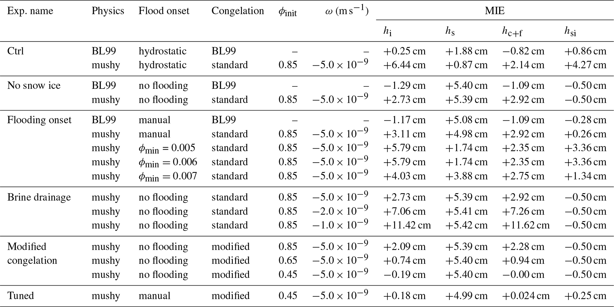
Table 1 Parameters and performance in mean integrated error (MIE) for all SIMBA1 simulations.

4.3 Experiment setup

Multiple Icepack simulations are run with the BL99 physics or the mushy-layer physics to reproduce each of the SIMBA observations. All simulations are initialized using the ice thickness, snow depth and internal ice temperature (at locations corresponding to the center of the snow and ice layers) recorded by the buoys. The initialization values are taken on 1 March, a few days after the SIMBA deployment to ensure that the deployment holes are completely refrozen. The simulations are run with seven ice layers, one snow layer and a time step of 1 h (outputs only every 3 h) from 1 March until well past the buoy recovery date. Results are only shown for the period corresponding with observation records.

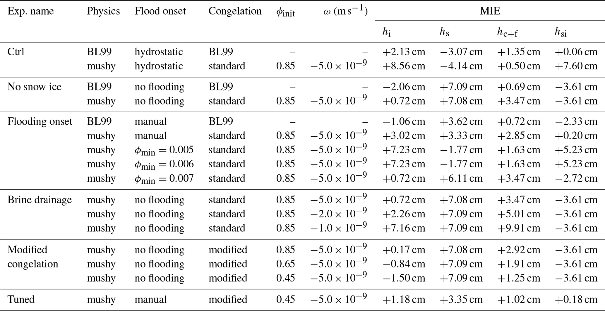
The parameter specifications for each simulations are listed in Tables 1 and 2 for the SIMBA1 and SIMBA2 experiments, respectively. Control simulations are first run using the default Icepack BL99 physics and mushy-layer parameterizations. A series of experiments are then conducted to investigate the influence of individual mushy physics components on the model performance by (1) removing the snow-ice parameterization, (2) adding a minimum liquid fraction (ϕ_min) criteria for snow flooding, (3) varying the strength of the brine drainage and (4) using the modified congelation scheme with varying initial liquid fraction ϕ_init.

Table 2 Parameters and performance in mean integrated error (MIE) for all SIMBA2 simulations.

4.4 Model evaluation

The performance of each simulation is quantified using the mean integrated error (MIE) of the ice thickness, snow depth, cumulative congelation and snow-ice formation. For each variable, the MIE is calculated first by linearly interpolating the SIMBA and simulation data into an hourly time series. The MIE is then defined as

$$\begin{array}{}\text{(37)}& \mathrm{MIE}=\sum _{\mathit{\tau }=\mathrm{1}}^n{\displaystyle \frac{(X_{\mathrm{sim}}^{\mathit{\tau }}-X_{\mathrm{obs}}^{\mathit{\tau }})}{n}},\end{array}$$

where n is the number of valid data points in the time series and $X_{\mathrm{sim}}^{\mathit{\tau }}$ and $X_{\mathrm{obs}}^{\mathit{\tau }}$ are the simulated and observed variable values at time τ in the interpolated time series.

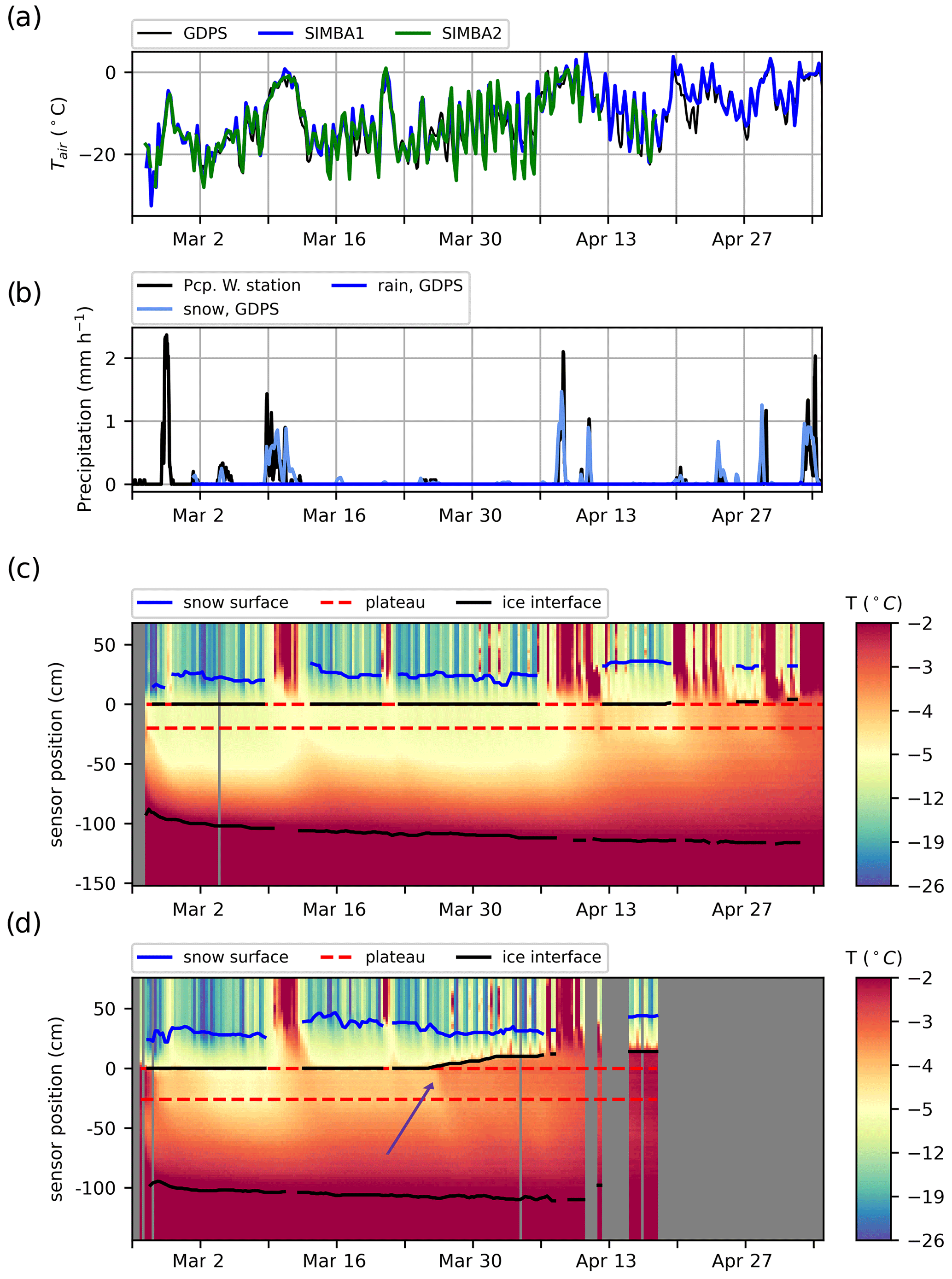
Figure 3 Time series of (a) air temperature from the GDPS (black) and recorded by the SIMBA buoys (SIMBA1 in blue, SIMBA2 in green), (b) precipitations from the Nain ECCC weather station (black) and from the GDPS (blue), (c) recorded temperatures along the SIMBA1 thermistor string with the detected material interfaces (air–snow interface in blue, ice interfaces in black and thermistor string plateau in red); (d) same as (c) but for the SIMBA2 buoy. The purple arrow points to the warming at the snow–ice interface, indicating flooding.

5 Results

5.1 In situ landfast ice thermodynamics

5.1.1 Observed temperature and weather conditions

The late-winter conditions along the Labrador coast are characterized by increasingly large diurnal cycles in air temperature, with longer (synoptic-scale) events of colder or warmer weather (Fig. 3a). The 2 m air temperatures calculated from the GDPS data correspond well with the air temperatures recorded in situ but are generally colder (MIE of −0.78 and −0.58 °C compared to the SIMBA1 and SIMBA2 records, respectively). These biases are mostly associated with differences in the short-term temperature peaks; the buoys record larger maxima in air temperatures than represented in the GDPS data.

Several precipitation events occurred during the observational periods. The snow precipitation events from the GDPS data correspond well with the precipitations recorded at a nearby weather station (Nain Airport; Fig. 3b). The precipitation phases were not documented in the airport records, and all events were snowfalls in the GDPS data. In particular, two events with heavy snowfalls are recorded on 9–11 March and on 6–10 April, which also correspond to periods of warmer weather during which temperatures slightly exceeded the freezing point.

The vertical temperatures recorded along the two SIMBA thermistor strings are coherent with these patterns (Fig. 3c–d). Short-term variations in air temperature are rapidly damped in the snow layer even though heat from longer periods of warm weather reaches, and has a larger impact on, the ice interior. The downward propagation of the surface heat is often followed by a slower cooling once colder conditions return. Despite the similar air temperature patterns, the SIMBA2 recorded significantly warmer ice temperatures than SIMBA1, with sharp warming events (see purple arrow in Fig. 3d) that suggest a snow-flooding onset (Provost et al., 2017).

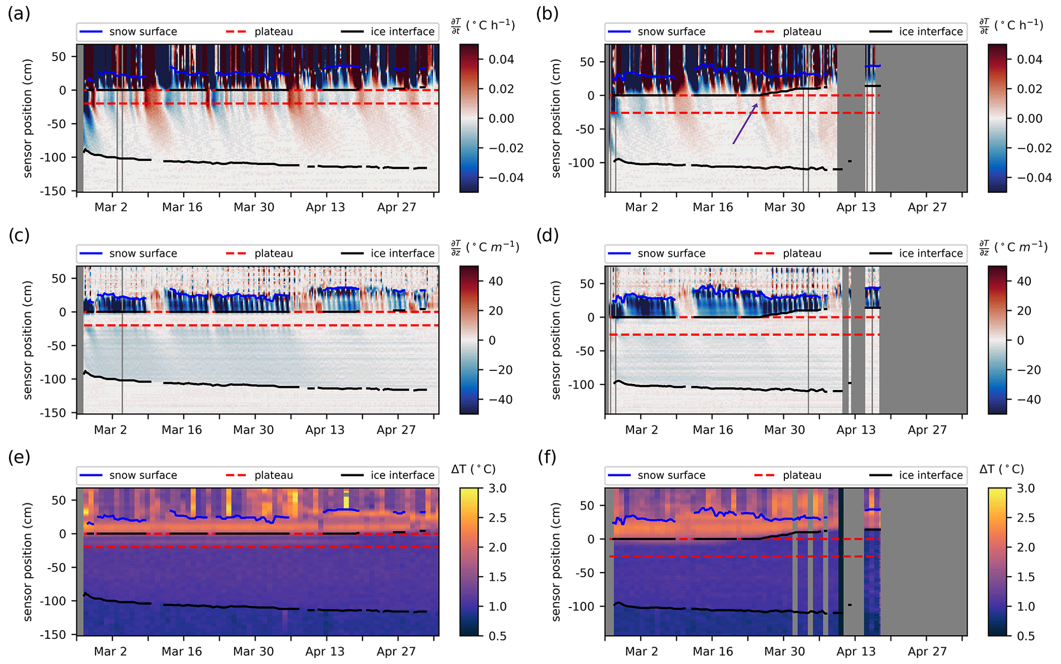
Figure 4 Rates of temperature changes (a, b), vertical temperature gradients (c, d) and change in temperature recorded after 2 min of heating during the daily heating cycles (e, f) at each sensor as measured for SIMBA1 (a, c, e) and SIMBA2 (b, d, f). Colored lines indicate the detected material interfaces (air–snow interface in blue, ice interfaces in black and thermistor string plateau in red). The purple arrow points to the warming at the snow–ice interface, indicating flooding.

5.1.2 Surface retrieval algorithm validation

The surface retrieval algorithm is able to identify the snow and ice interfaces in most of the records (Fig. 3c–d). The algorithm fails during the two warm spells when negligible vertical temperature gradients or temperature inversions are present within the snow and ice layers (i.e., the piecewise linear assumption does not hold). The surface retrieval algorithm is also generally not successful during the melt season (beyond 16 April) for the same reason, except on occasional colder days.

While we do not have independent data to validate the retrieved snow and ice thicknesses, we find that the selected interfaces are coherent with the interfaces detectable by visual inspection in the temperature profiles (Fig. 3c–d). The detected snow interfaces correspond well with the layer within which most of the variability associated with diurnal cycles or synoptic systems is damped (Fig. 4a–b) and where large vertical temperature gradients are present (Fig. 4c–d). The algorithm detects an upward migration of the snow–ice interface (i.e., snow flooding; see the upward displacement of the top black line, representing the snow–ice interface, above its original position) that also corresponds well with the warm temperatures recorded above the initial ice surface. In particular, the onset of flooding at the SIMBA2 site (on 26 March) coincides with a sudden warming event observed at the snow–ice interface, propagating upward in the snow layer despite a cooling in the surface air temperature above (see profiles at the purple arrow in Figs. 3d and 4b). This signal is expected when the snow flooding is caused by upward percolation or lateral advection of seawater (Provost et al., 2017), since the warm seawater increases the snow–ice interface temperature, and the heat later diffuses upward. In contrast, flooding by liquid precipitation or snow melting would show the entire snow layer at the freezing point. This could be the case at the SIMBA1 site, where flooding is only detected late in the observational record (on 25 April) when surface air temperatures above freezing are regularly present.

The top and bottom ice interfaces show good agreement with those seen in the recorded warming of sensors during the SIMBA heating cycles (Fig. 4e–f). The detected snow layers are also coherent with the thermistor string sections measuring the largest heating (smallest conductivity), although this is more difficult to assess with certainty due to the large variations within this layer, likely resulting from a vertically varying snow density. Note that the SIMBA2 heat cycle records (Fig. 4f) present a rather smooth vertical gradient over 2–4 cm within the thermistor plateau, supposedly sitting on the snow–ice interface. We speculate that this is due to the thermistor plateau not being exactly horizontal on the ice surface, indicating a (∼1–2 cm) thickness uncertainty related to this deployment method for a marking of the initial ice surface. This positional uncertainty remains for the entire record but is no longer visible once the thermistor plateau is flooded.

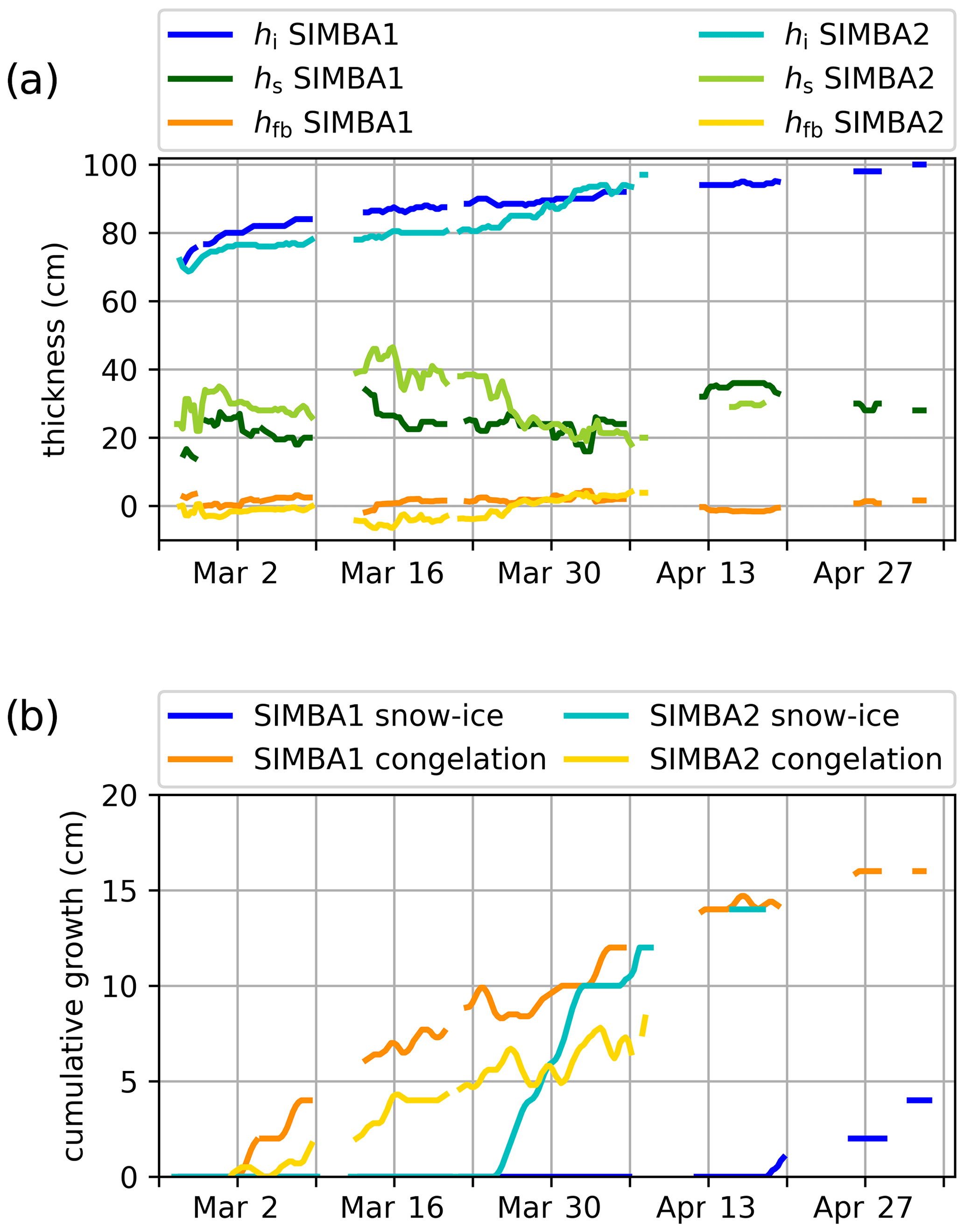
Figure 5 (a) Ice (blue lines), snow (green lines) and freeboard (orange lines) thicknesses from the SIMBA data. (b) Contribution of snow ice (blue lines) and congelation ice (orange lines) to the ice mass balance inferred from the SIMBA data.

5.1.3 In situ landfast ice mass balance

The SIMBA observations show large snow depths (∼20–40 cm) over relatively thin ice (∼75–100 cm) from the beginning of the records, and the measured freeboard occasionally dips to negative values (Fig. 5a). Both sites present significant snow depth increases during each warm event with a subsequent reduction likely resulting from snow compaction and redistribution by winds. The snow depths are generally larger at the SIMBA2 site (by ∼5–10 cm), with a large but short-lived maximum of 50 cm likely resulting from snow accretion and subsequent removal by the winds around the buoy.

The local ice mass balance at the two sites is largely influenced by the snow layer thickness and its insulating effect on the sea ice below. The thinner snow cover at the SIMBA1 site results in colder internal ice temperatures, larger congelation rates at the ice base and less snow flooding (Fig. 5b). With an initial ice thickness and snow depth of 80 and 26 cm, respectively (on 1 March), the SIMBA1 freeboard reaches negative values after each snowfall event: −1.8 cm on 13 March and −1.6 cm on 14 April. Snow flooding is only detected from 25 April onward. The ice thickness reached its maximum (100 cm) on 1 May, for a total ice growth of 20 cm, from which 16 cm is associated with (downward) congelation at the ice–ocean interface and 4 cm is associated with (upward) snow-ice formation. In comparison, the SIMBA2 buoy initially recorded a 30 cm snow depth and 76 cm ice thickness (on 1 March), already corresponding to a negative freeboard (−1.6 cm). Snowfalls during the first warm event brings the freeboard to a minimum of −6.4 cm on 15 March. Snow flooding is detected from 25 March onward, coinciding with a large (∼10 cm) reduction in the snow depth. By 6 April, the ice thickness reached a maximum of 97 cm for a total ice growth of 21 cm, 13 cm of which is attributed to snow-ice formation and 8 cm to congelation.

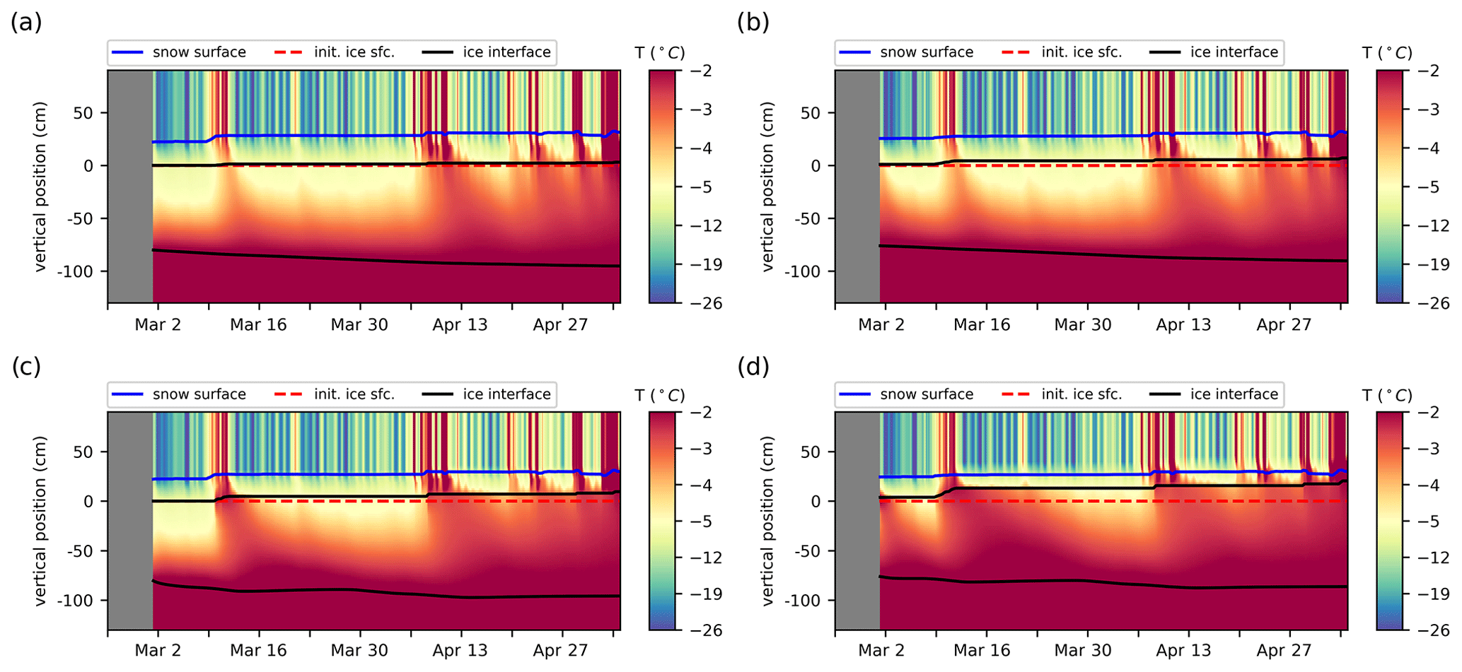
Figure 6 Simulated internal temperatures interpolated into 2 cm intervals from the BL99 (a, b) and mushy simulations (c, d), initialized from the SIMBA1 (a, c) and SIMBA2 (b, d) data. Solid lines indicate the simulated material interfaces (air–snow interface in blue, ice interfaces in black).

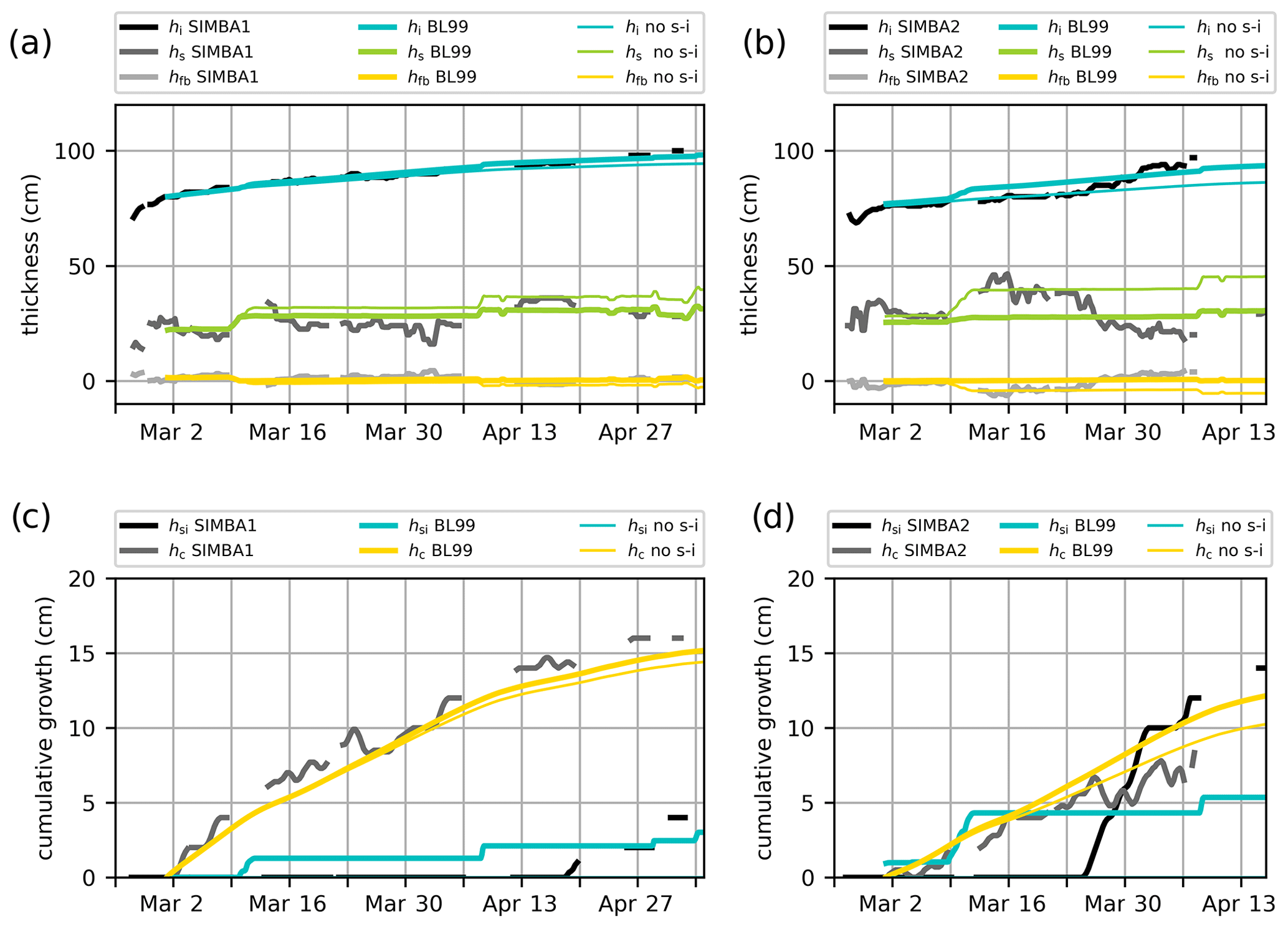
Figure 7 Ice mass balance in the BL99 simulations against the SIMBA1 (a, c) and SIMBA2 (b, d) observations. Top panels (a, b) represent ice thickness (blue lines), snow depth (green lines) and freeboard (yellow lines) values, with the observations in black. Bottom panels (c, d) represent cumulative ice growth from ice bottom (yellow lines) and snow-ice formation (blue lines), with the observations in black. Thin lines indicate results from the BL99 simulation ran without using the snow-ice parameterization.

5.2 BL99 simulations

The BL99 thermodynamics represents generally well the observed internal temperature profiles but with a larger downward heat conduction in the ice interior during periods of warm weather compared to the observations (Fig. 6). The simulated snow thicknesses present large discrepancies with observations (MIE of +1.88 and −3.07 cm for SIMBA1 and SIMBA2, respectively), with a tendency to remain mostly constant except for the occasional increases associated with precipitation events. This is mostly due to the simple snow model not accounting for snow compaction and redistribution. The simulated ice thickness is in general accord with observations (Fig. 7a–b) with a small positive bias +0.25 cm (MIE) for SIMBA1 and +2.13 for SIMBA2 (see Tables 1 and 2). Despite the positive MIE values, the ice thickness at the time of the observed maximum is smaller than the observed values, at 97.4 and 90.8 cm for the SIMBA1 and SIMBA2 simulations, respectively (−2.6 and −6.2 cm underestimations). Most of the ice growth is attributed to ice congelation at the ice bottom (14.9 and 10.5 cm), showing slowly decreasing ice growth rates from ∼0.3 cm d⁻¹ to near zero in May. The volume of snow ice is largely underestimated at 2.4 and 4.3 cm (−1.6 and −8.7 cm underestimations) despite the fact that conditions for snow-ice formation are met from the very start of the simulation (Fig. 7c–d).

The ice thickness and snow depth discrepancies are partly attributed to the misrepresentation of snow-ice formation, specifically to the hydrostatic-balance-based snow-flooding onset: the initialized snow depths are sufficient enough to depress the ice surface near (or already below in the SIMBA2 case) the water line, with any subsequent snow precipitation leading to a portion of the snow cover being immediately transformed into snow ice (see orange lines representing the freeboard values in Fig. 7a–b and blue lines representing the snow-ice volumes in Fig. 7c–d). This leads to the ice thickness temporarily exceeding the observations early in the simulations up to the observed snow-flooding onset, after which the thickness bias turns negative (in the SIMBA2 case) due to the small snow-ice volume.

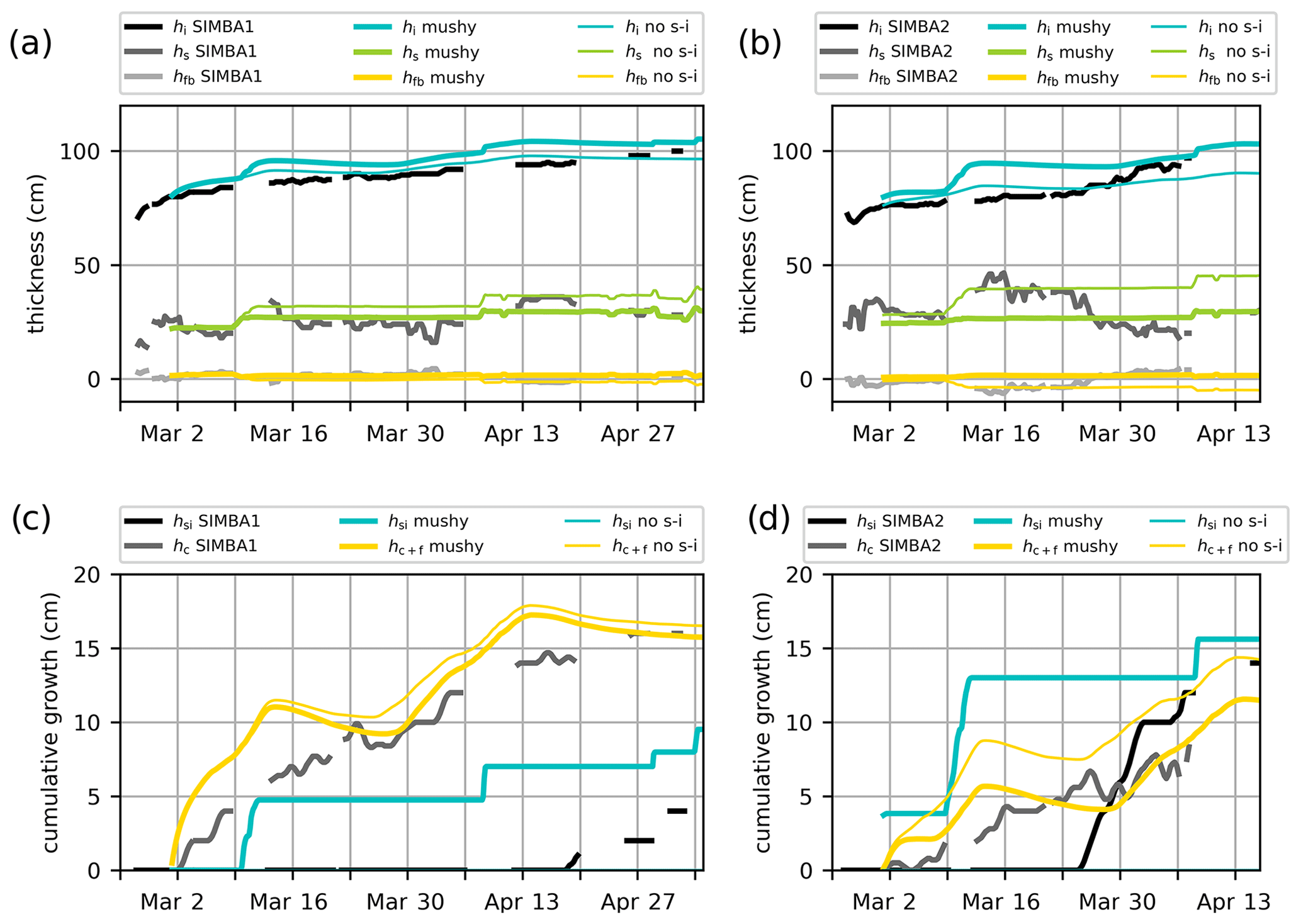
Figure 8 Ice mass balance in the mushy-layer simulations against the SIMBA1 (a, c) and SIMBA2 (b, d) observations. Top panels (a, b) represent ice thickness (blue lines), snow depth (green lines), and freeboard (yellow lines) values, with the observations in black. Bottom panels (c, d) represent cumulative ice growth from ice bottom (yellow lines, including frazil) and snow-ice formation (blue lines), with the observations in black. Thin lines indicate results from the mushy simulations run without using the snow-ice parameterization.

5.3 Mushy simulations

Compared to the BL99 simulations, the mushy-layer physics produces warmer sea ice temperatures (see Fig. 6c–d) and faster ice growth at both interfaces (i.e., upward snow-ice formation and downward bottom ice growth; see Fig. 8). These differences are present despite the fact that the simulated snow depths are very similar in both simulations.

The ice thickness in the mushy simulations reached 103.8 and 97.5 cm for SIMBA1 and SIMBA2, respectively, at the time of the observed maximum, corresponding to 3.8 and 0.5 cm overestimations. The ice growth presents larger variations than observations due to a combination of spurious snow-ice formation and variable basal ice growth. The spurious snow-ice formation is similar to but larger than in the BL99 simulations, yielding large ice thickness discrepancies during the period with observed negative freeboards. The total volume of snow ice is, however, closer to observations, with 8.0 and 13.0 cm for the SIMBA1 and SIMBA2 simulations, respectively (+4.0 and 0.0 cm deviations from observations). The basal growth variability could be considered an asset when compared with the slowly varying congelation rates in the BL99 simulations, but it is largely overestimated and effectively degrades the model performance. In particular, the simulated basal growth features periods of weak basal melt that are not coherent with observations (Fig. 8c–d). Furthermore, a quarter of the basal growth is attributed to the frazil formation during periods of rapid congelation (see the Appendix A). This frazil formation occurs despite the landfast ice conditions with a 100 % sea ice concentration and uniform thickness and is related to the treatment of the ice–ocean boundary in the mushy-layer congelation parameterization (see Sect. 3.2.2 and Appendix for details).

All control simulations (BL99 and mushy) thus present discrepancies early in the simulations due to the hydrostatic-balance criteria not accounting for negative freeboards. This difficulty lead Duarte et al. (2020) to manually activate/deactivate the snow-ice parameterization (i.e., by adding/removing the condition of the hydrostatic equilibrium according to the observations) to adequately reproduce in situ conditions. In our experiment, deactivating the snow-ice parameterization in all simulations effectively allows the snow depth to increase during precipitation events (see thin green lines in Figs. 7 and 8) and reduces the ice thickness discrepancy up to the flooding onset (thin blue lines in Figs. 7 and 8). This, however, leads to an underestimation of the ice thickness by the end of the simulations due to the missing snow-ice contribution in the ice mass balance.

The removal of snow-ice formation causes different responses in the BL99 and mushy-layer thermodynamics. Using the BL99 physics, simulations without snow ice show smaller congelation rates due to the increased insulation from the larger snow depths. Using the mushy-layer physics, simulations without snow ice show larger congelation rates despite the larger snow depths, since the ice interior is colder without the influx of warm ocean water associated with flooding, resulting in larger conductive heat fluxes at the ice base.

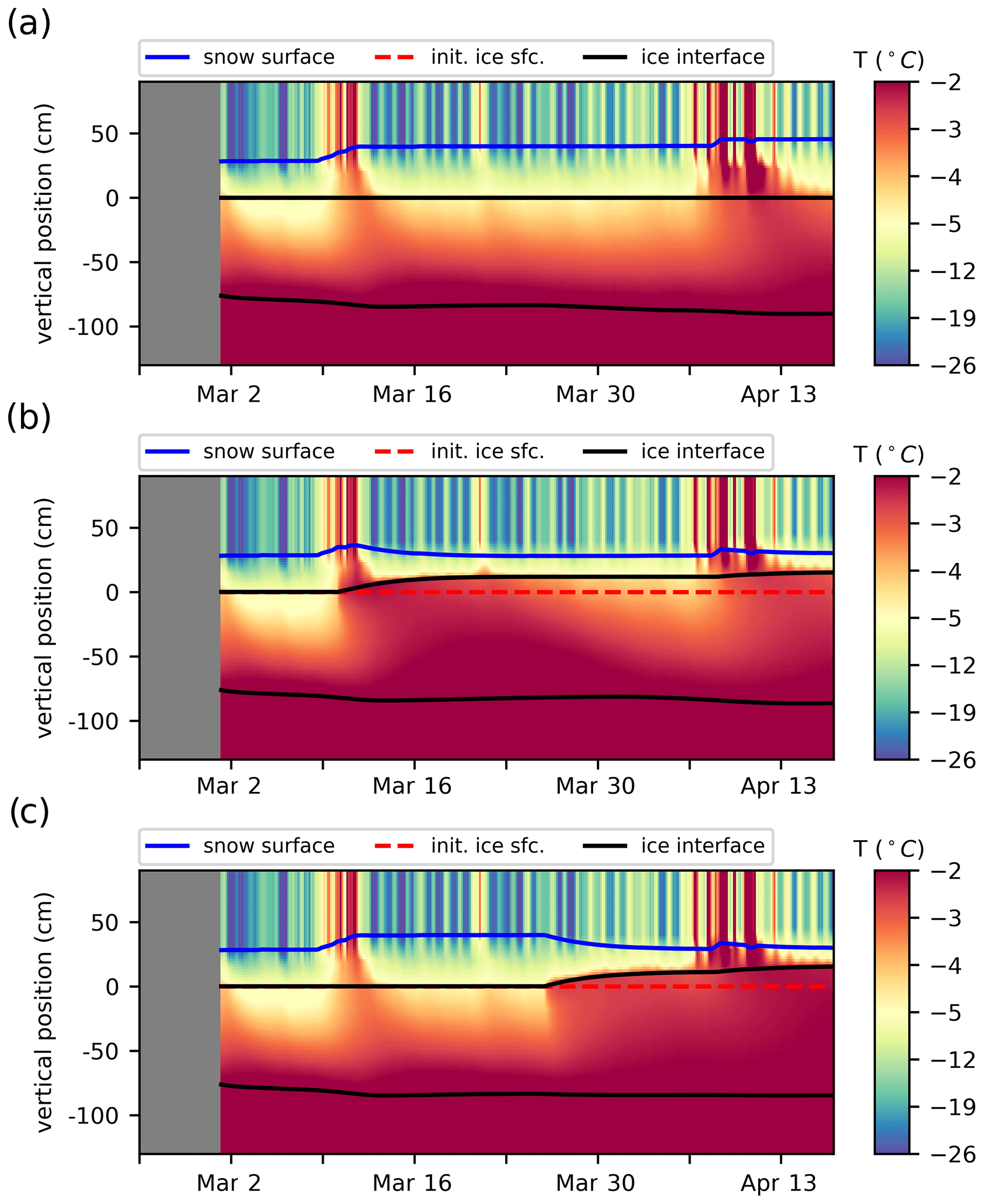
Figure 9 Time series of the simulated vertical temperature profiles interpolated in 2 cm intervals to reproduce the SIMBA2 records using the mushy-layer physics with different criteria for snow flooding. Thick lines indicate the material interfaces (air–snow in blue, ice interfaces in black and the initial snow–ice interface in dashed red). (a) Without snow flooding, (b) using ϕ=0.005 as a snow-flooding onset criteria and (c) manually setting the snow-flooding onset on 26 March to match the observations.

We note that while the mushy-layer simulations quantitatively represent a degradation of the model performance (see larger MIE values in Tables 1 and 2), this is largely due to the snow-flooding onset discrepancy combined with the wider-ranging effects of the flooding on the ice thickness growth, interior ice salinity and temperatures. These effects, however, are physically meaningful and correspond well with previously recorded thermodynamics of snow flooding (see Provost et al., 2017, for instance). This suggests that the model performance could be largely improved by a simple tuning of the snow-flooding onset and rates. For instance, we find that adding a simple minimum porosity criterion (ϕ_min=0.005) to the snow-ice parameterization and setting the flooding rate inversely proportional to h_fb largely improves the SIMBA2 simulations by delaying the snow-ice formation by several days (Fig. 9b). The model in particular presents very small MIE values for snow-ice formation when the flooding onset is set manually to the observed date (Fig. 9c and Table 2).

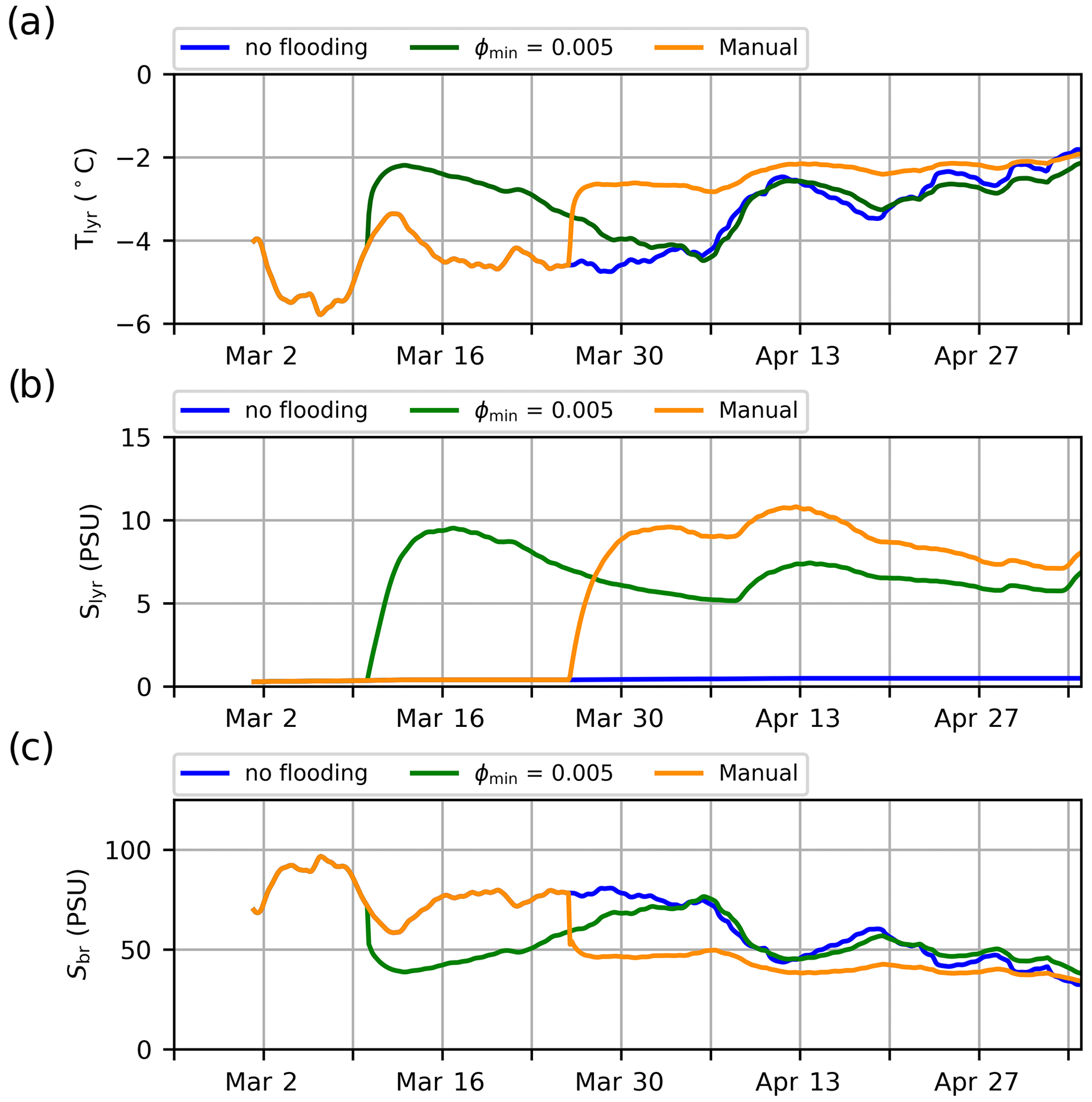
Figure 10 Time series of the (a) temperature, (b) bulk salinity and (c) brine salinity in the upper ice layer in mushy simulations with different criteria for snow-ice formation (blue lines represent no flooding).

5.4 Basal ice temperature, brine salinity and congelation

The inclusion of prognostic salinity and brine parameterizations in the mushy-layer physics adds model sensitivities relating to the liquidus relationship. That is, for a given salinity, the liquidus relation interconnects changes in temperature with changes in brine salinity and liquid fraction. As such, updating the brine salinity in explicit parameterizations, such as the snow-flooding parameterizations or ice congelation parameterizations, later affects the layer temperature solved implicitly in subsequent time steps. For instance, the seawater added in the upper ice layer in the snow-ice parameterization increases the layer bulk salinity but also dilutes the brine salinity towards SSS values. This effectively warms the layer according to the liquidus balance (Fig. 10). The layer temperature then slowly returns to colder values as the brine pockets refreeze, concentrating the brine salinity to its original value (see curves converging back to values from the negative freeboard simulations in Fig. 10a).

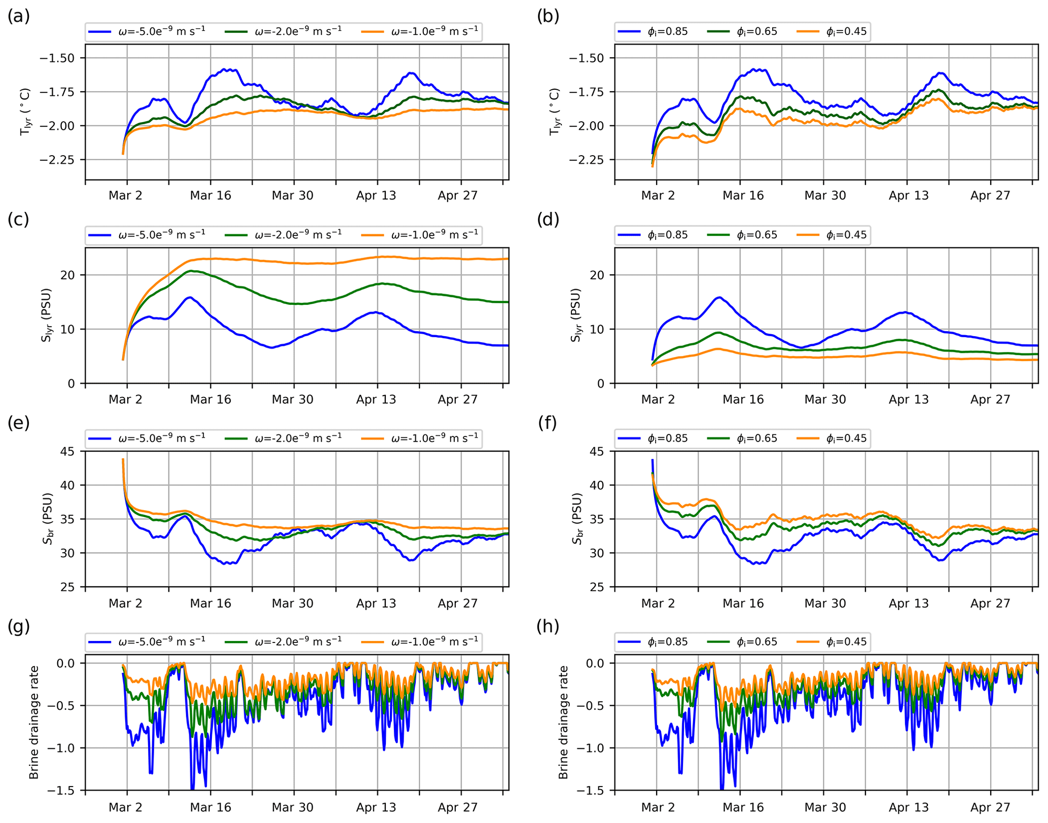
Figure 11 Time series of the temperature (a, b), bulk salinity (c, d), brine salinity (e, f) and brine desalination rate from the slow-brine-drainage parameterization (g, h, represented in psu d⁻¹), all in the lowest ice layer. Left panels showy mushy-layer simulations using different brine drainage strength parameters ω (using the standard congelation). Right panels show mushy-layer simulations using the different initial congelation liquid fraction ϕ_init and using the modified mushy-congelation scheme.

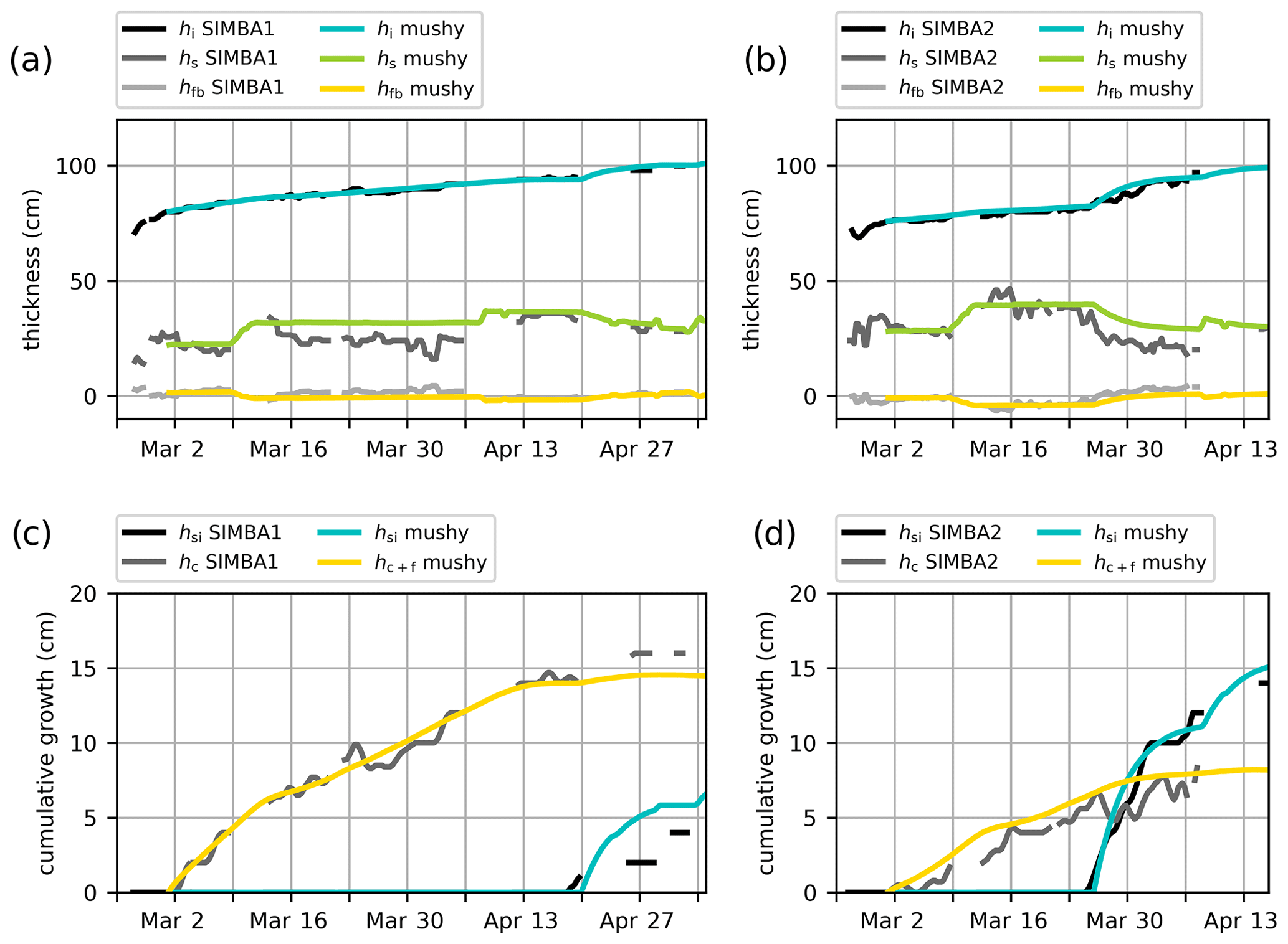
Figure 12 Ice mass balance in mushy-layer simulations tuned to best represent the observations from the SIMBA1 (a, c) and SIMBA2 (b, d) buoys (observations are in black). The snow-flooding onset is set manually according to the observed flooding onset dates, and the simulations use the modified congelation scheme with ϕ_init=0.45. Top panels (a, b) show ice thickness (blue lines), snow depth (green lines) and freeboard (yellow lines) values. Bottom panels (c, d) show cumulative ice growth from ice bottom (yellow lines, including frazil) and snow-ice formation (blue lines).

Similarly, the alternating periods of sea ice congelation and melt in the standard mushy-layer simulations are attributed to a similar brine–temperature feedback in the lowest ice layer: any process reducing the brine salinity yields an increase in the layer temperature T_n. This reduces the conductive flux at the ice base (see Eq. 7, with T_f constant at the freezing point) and thus the available energy for congelation. Specifically, there are two explicit parameterizations inducing brine salinity changes at the ice base in the mushy-layer thermodynamics: the brine drainage parameterizations (reducing the brine salinity) and the ice congelation parameterizations (diluting the brine towards the SSS). These parameterizations together bring the brine salinity close to SSS values early in the simulations (see blue curve in Fig. 11c for the control simulation). Later, brine drainage under cold weather further dilutes the brine to values below the SSS (and thus, T_n>T_f), causing a reversal of the conductive flux and sea ice melt. This pattern can be suppressed by reducing the strength of the brine drainage (reducing the parameter ω, Fig. 11, left panels), although it also consequently yields too large congelation rates.

The basal ice growth can be improved by modifying the congelation parameterization to reduce the associated salinity increase (Fig. 11b, d, f and h). To do so, we repeat the experiments using a modified congelation scheme in which a mush layer with a liquid fraction ϕ_init and S_br= SSS is incorporated in the lowest ice layer during congelation (see Sect. 3.2.3 and Appendix B). Using this scheme, reducing the liquid fraction of congelation ice (ϕ_init) results in smaller congelation rates and salinity in the lowest ice layer. This in turn reduces the strength of the brine drainage (a lower salinity in Eq. 15), diminishing the variations in congelation while bringing the congelation rates closer to observations.

6 Discussion and conclusions

In this study, the thermodynamic growth of landfast ice in the vicinity of Nain (Labrador) is investigated from two Scottish Association for Marine Science (SAMS) snow ice mass balance apparatus (SIMBA) buoys deployed in winter 2017. The observed thermodynamics are reproduced using Icepack (v1.1.0), which is the column thermodynamics package of the Community Ice CodE (CICE) version 6, with two different physical schemes: the Bitz and Lipscomb (1999) physics that represent the thermodynamics currently used in the Environment and Climate Change Canada (ECCC) ice–ocean forecasting systems and the mushy-layer thermodynamics (Feltham et al., 2006; Notz and Worster, 2009; Turner et al., 2013) that include new physics available in CICE6. The performance of Icepack in reproducing the IMB observations is assessed with particular attention to the improvements associated with the use of the mushy-layer physics. The contributions of this paper include a new automated surface retrieval algorithm to infer the ice and snow thicknesses from thermistor string records, a modified mushy-layer congelation scheme less conducive to frazil formation and modifications to the snow-flooding parameterization to allow for negative freeboards and slow snow flooding rates.

The in situ observations presented in this analysis are in line with a number of negative freeboard measurements reported in recent years in the Arctic (Rösel et al., 2018; Provost et al., 2017; Duarte et al., 2020), which are likely to become more frequent as the sea ice thins and precipitation increases in the transition to a seasonal ice cover (Merkouriadi et al., 2020). Snow flooding remains nonetheless relatively infrequent: our in situ snow flooding observations were associated with anomalous 2017 snow conditions that have not yet reoccurred in subsequent (2018–2023) landfast ice observation campaigns. The frequency at which snow flooding contributes to the ice mass balance in landfast ice areas, in Nain but also more widely along the Canadian Arctic, remains to be determined. Note, however, that as snow-ice formation occurs more easily over thin ice (Granskog et al., 2017), it is likely contributing to the ice growth early in the season and in new leads. This could be better assessed with IMB buoys deployed in open water prior to the freeze-up. Such a deployment was attempted in 2022 in Nain, but buoy icing, floe drifting and wave battering prevented the measurement of a continuous time series during the freeze-up period.

The large discrepancies between the observed and simulated snow-flooding onset in the analysis join the results of Duarte et al. (2020) in demonstrating that the use of the hydrostatic balance alone is insufficient to define snow flooding and to capture the more complex processes observed in situ (Eicken et al., 1995; Maksym and Jeffries, 2000; Provost et al., 2017). Our results show that while this conclusion also applies to the BL99 parameterization, the snow flooding exerts a much wider-ranging thermodynamic response under the mushy-layer physics as the flooding increases the temperature, salinity and liquid fraction in the upper ice layers. It better represents the observed thermodynamics and is an improvement compared to the BL99 physics, as indicated by the smaller MIE values when the flooding onset is corrected according to the observations (see Table 2). One advantage of the mushy-layer physics is that it contains the necessary ingredients to improve the snow-flooding parameterization with additional porosity conditions for the percolation of seawater through the brine channels.

In our analysis, no porosity criterion was found to reproduce the observed snow-flooding onset date. This could indicate the influence of nearby sea ice dynamics, although in our case, the deployed IMBs were located in a well-sheltered landfast channel dozens of kilometers away from the landfast ice edge. Moreover, the slow rate of snow-ice formation corresponds well with percolation through the porous sea ice medium (i.e., as opposed to the sudden flooding expected when floodwater is advected laterally from neighboring deformation sites; Provost et al., 2017). One difficulty in reproducing the snow-flooding onset with porosity criteria is that they do not account for a percolation associated with the larger-scale porosity (e.g., from thermal cracking) unrelated to the smaller-scale mushy-layer characteristics. At the kilometer scale of most dynamic sea ice models, the volume of snow ice will likely not be uniform over a grid-cell area. This is made evident in our results by the different in situ flooding onset recorded by our two neighboring SIMBAs. Most likely, the snow-ice volume will be spatially distributed according to the ability of the floodwater to penetrate the snow layer, ultimately depending on the ice topography (ice thickness distribution), local snow conditions and the ice heterogeneity (i.e., the presence and average distance between cracks). The snow-ice volume at this scale would thus likely be better represented by a subgrid parameterization relating the snow conversion to a spatial probability for water penetration.

Our results further demonstrate that the mushy-layer physics leads to a much larger salinity and temperature variability at the ice bottom, with significant sensitivity to new free parameters (e.g., ω, ϕ_init). This highly impacts the simulated ice congelation rates and, using the default Icepack parameters, yields a degradation of the model performance despite the improved representation of brine processes. This performance is, however, mostly associated with the treatment of the brine salinity in the explicit congelation parameterization producing overinflated congelation rates, erroneous melt and significant frazil formation. The frazil formation in particular is not expected in our sheltered landfast context, but its overrepresentation is coherent with previous studies reporting large frazil volumes in pan-Arctic or Antarctic simulations using the mushy-layer thermodynamics (Turner and Hunke, 2015; Bailey et al., 2020; DuVivier et al., 2021).

The mushy-layer thermodynamics can, nonetheless, outperform the BL99 simulations using a simple modification to the congelation parameterization with a tuning of the initial congelation liquid fraction. Note, however, that the modified congelation is not salt-conserving (i.e., similar to the frazil formation) and should be treated accordingly in the context of coupled simulations. The best model performance was obtained when the mushy-layer physics was used with the modified congelation parameterization, a reduced initial congelation liquid fraction and a manual snow-flooding onset (Fig. 12). We note, however, that this represents significant tuning towards our SIMBA observations, which are not representative of typical high-Arctic conditions. As such, this tuning exercise is not meant to determine specific parameter values to be used in Icepack. It nonetheless demonstrates the need to better constrain the mushy-layer parameters, which could be made in future work with larger sets of in situ observations including salinity measurements.

Finally, we note that the increased sensitivity to physical processes in the mushy-layer thermodynamics is likely to positively affect the landfast ice dynamics. For instance, the larger congelation rates simulated under conditions of colder air may allow for faster sea ice consolidation (increasing the effective ice strength) and ease the formation of ice arches in narrow passages. The impact of snow flooding, precipitation and surface melt on the ice interior via brine dynamics is also likely to increase the preconditioning from large-scale ice strength heterogeneity early in the thaw season, which also could affect the landfast ice variability and the timing of its breakup. The mushy-layer thermodynamics thus presents itself as a useful, if not necessary, step towards improving the coupling between the thermodynamic and dynamic sea ice model components.

Appendix A: Frazil formation from the standard mushy-layer congelation parameterization

In Icepack, the mushy-layer congelation parameterization is composed of two components: the downward migration of the ice–ocean boundary, based on the computed congelation rate, and the integration of mass (seawater and/or fresh ice) in the bottom sea ice layer. In mushy-layer physics, the ice–ocean interface is defined by the position where the mush medium reaches a 100 % liquid fraction. Accordingly, the standard congelation parameterization assumes that its downward migration precedes the freezing of seawater, such that seawater without fresh ice is being added in the mush medium. Later, solidification in the bottom ice layer occurs in subsequent time steps when solving for the internal temperature profiles via the liquidus relation. This, however, implies that the enthalpy used to define the congelation rate (i.e., Eq. 16, based on initial congelation liquid fraction ϕ_init) differs from the energy actually being integrated in the sea ice by congelation.

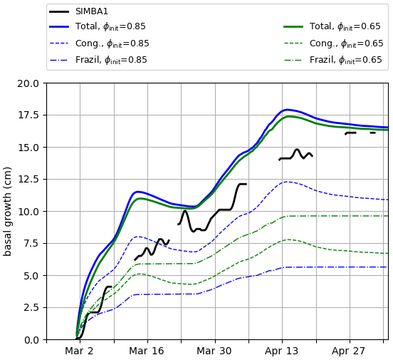
Figure A1 Total basal ice growth (h_c+f, solid lines) and contributions from congelation (h_c, dashed lines) and frazil formation (h_f, dot-dashed lines) in mushy simulations using the standard congelation scheme, with different initial congelation liquid fractions: default ϕ_init=0.85 in blue and ϕ_init=0.65 in green.

Specifically, defining $E_{\mathrm{A}}=F_{\mathrm{bot}}-F_{\mathrm{cb}}$ as the energy available for congelation (i.e., the conductive heat imbalance at the ice–ocean interface) and E_U as the energy used during congelation (i.e., from Eq. 17), the fraction r of the available energy used by the mushy-layer congelation can be written as

$$\begin{array}{}\text{(A1)}& r={\displaystyle \frac{E_{\mathrm{U}}}{E_{\mathrm{A}}}}={\displaystyle \frac{-q_{\mathrm{w}}\frac{\partial h_{\mathrm{c}}}{\partial t}}{F_{\mathrm{bot}}-F_{\mathrm{cb}}}},\end{array}$$

where h_c is the congelation ice thickness and q_w=c_wρ_wT_f is the enthalpy of seawater at the freezing point. Using Eq. (16), this reduces to

$$\begin{array}{}\text{(A2)}& \begin{array}{rl}r& ={\displaystyle \frac{q_{\mathrm{w}}}{-L_{\mathrm{0}}{\mathit{\rho }}_{\mathrm{i}}(\mathrm{1}-{\mathit{\varphi }}_{\mathrm{init}})}}\\ & =-c_{\mathrm{1}}{\displaystyle \frac{T}{\mathrm{1}-{\mathit{\varphi }}_{\mathrm{init}}}},\end{array}\end{array}$$

where c₁=ρ_wc_w/L₀ρ_i∼0.014 and T is in degrees Celsius. This demonstrates that unless ϕ_init is close to 1, the congelation only accounts for a fraction r≪1 of the heat flux imbalance (e.g., using ϕ_init=0.85 and $T\sim -\mathrm{1.8}\mathit{°}$C, we find r=0.17), and the remaining energy is taken from the ocean. If the ocean is at the freezing point and there is no heat transfer from below the mixed layer, this energy transfer leads to frazil formation. The rate of frazil formation can be estimated using Eq. (19) with $F_{\mathrm{ocn}}=(\mathrm{1}-r)U_{\mathrm{A}}$, as

$$\begin{array}{}\text{(A3)}& {\displaystyle \frac{\partial h_{\mathrm{f}}}{\partial t}}={\displaystyle \frac{\mathrm{1}-r}{-q_{\mathrm{f}}}}{E}_{\mathrm{A}}.\end{array}$$

The total basal ice growth in the standard mushy-layer physics is then obtained by adding Eqs. (16) and (A3):

$$\begin{array}{}\text{(A4)}& \begin{array}{rl}{\displaystyle \frac{\partial h}{\partial t}}& ={\displaystyle \frac{\partial h_{\mathrm{c}}}{\partial t}}+{\displaystyle \frac{\partial h_{\mathrm{f}}}{\partial t}}\\ & ={\displaystyle \frac{r}{-q_{\mathrm{w}}}}{E}_{\mathrm{A}}+{\displaystyle \frac{\mathrm{1}-r}{-q_{\mathrm{f}}}}{E}_{\mathrm{A}},\end{array}\end{array}$$

where Eq. (A2) has been used to rewrite the growth in terms of the available energy and the fraction r. This indicates that increasing the fraction r (e.g., by decreasing ϕ_init; see Eq. A2) decreases the congelation rate but also increases the amount of frazil formation by a proportional amount. Varying ϕ_init thus results in a similar total basal growth (Fig. A1).

Appendix B: Modified mushy-layer congelation parameterization

Here, we propose a modified mushy-layer congelation scheme that aims to reduce the amount of frazil formation. The modifications are twofold: (1) the congelation rate is defined by the energy needed to bring seawater enthalpy to that of the integrated mushy layer and (2) the mushy layer integrated in the lowest ice layer has a liquid fraction ϕ_init. This implies that some solidification occurs simultaneously as the ice–ocean interface migrates downward.

Specifically, instead of Eqs. (16) and (17), we use Eqs. (20) and (21). The energy integrated in the bottom ice layer in this case corresponds to

$$\begin{array}{}\text{(B1)}& E_{\mathrm{U}}=-q_{\mathrm{m}}{\displaystyle \frac{\partial h_{\mathrm{c}}}{\partial t}},\end{array}$$

and the fraction r of the available energy used by the modified mushy-layer congelation is (instead of Eq. A2) represented as

$$\begin{array}{}\text{(B2)}& \begin{array}{rl}r& ={\displaystyle \frac{-q_{\mathrm{w}}\frac{\partial h_{\mathrm{c}}}{\partial t}}{F_{\mathrm{bot}}-F_{\mathrm{cb}}}}\\ & ={\displaystyle \frac{q_{\mathrm{m}}}{q_{\mathrm{m}}-q_{\mathrm{w}}}}.\end{array}\end{array}$$

Given that q_m≪q_w (q_m and q_w being negative), we have r∼1, and the volume of frazil associated with congelation is negligible.

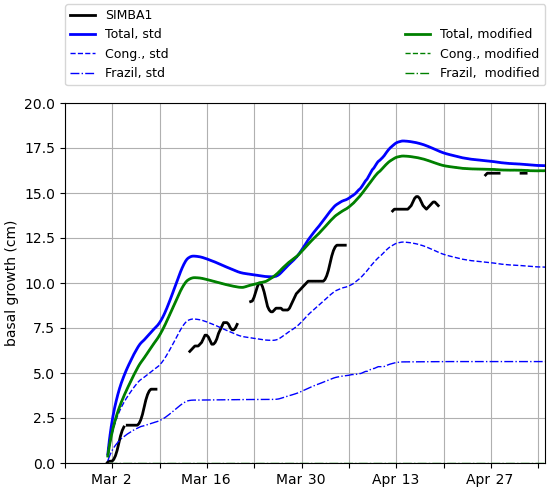
Figure B1 Total basal ice growth (h_c+f, solid lines) and contributions from congelation (h_c, dashed lines) and frazil formation (h_f, dot-dashed lines) in mushy simulations using the standard (blue) and modified (green) congelation schemes, both with default ϕ_init=0.85. Using the modified congelation scheme, the total basal growth and congelation lines are superposed as the frazil formation is zero.

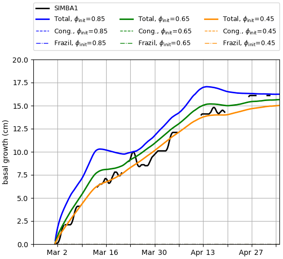
Figure B2 Total basal ice growth (h_c+f, solid lines) and contributions from congelation (h_c, dashed lines) and frazil formation (h_f, dot-dashed lines) in mushy simulations using the modified congelation scheme, with a different initial congelation liquid fraction. The total basal growth and congelation lines are superposed as the frazil formation is zero.

Using ϕ_init=0.85, the modified congelation schemes produce total basal growth rates similar to the ones simulated by the standard parameterization, but all of the growth is attributed to the congelation as there is only a negligible frazil formation (Fig. B1). The sensitivity to the parameter ϕ_init is, however, increased (Fig. B2), as the changes in ice congelation rates are no longer balanced by changes in frazil formation. This allows for better tuning with the observations.

Note that in this analysis, we define S_br= SSS to satisfy the liquidus at the boundary where T=T_f. This implies some salt rejection associated with congelation, and it should be treated accordingly when coupling with an ocean model. To keep the congelation salt-conserving, the brine salinity of the integrated mush layer could be set to $S_{\mathrm{br}}=\mathrm{SSS}/{\mathit{\varphi }}_{\mathrm{init}}$. Note, however, that this does not satisfy the liquidus at boundary and would thus affect the simulated temperature in the lowest ice layer.