the Creative Commons Attribution 4.0 License.
the Creative Commons Attribution 4.0 License.
 | 04 Apr 2024
Characterizing sub-glacial hydrology using radar simulations
Chris Pierce
Christopher Gerekos
Mark Skidmore
Lucas Beem
Don Blankenship
Won Sang Lee
Ed Adams
Choon-Ki Lee
Jamey Stutz
The structure and distribution of sub-glacial water directly influences Antarctic ice mass loss by reducing or enhancing basal shear stress and accelerating grounding line retreat. A common technique for detecting sub-glacial water involves analyzing the spatial variation in reflectivity from an airborne radar echo sounding (RES) survey. Basic RES analysis exploits the high dielectric contrast between water and most other substrate materials, where a reflectivity increase ≥ 15 dB is frequently correlated with the presence of sub-glacial water. There are surprisingly few additional tools to further characterize the size, shape, or extent of hydrological systems beneath large ice masses.
We adapted an existing radar backscattering simulator to model RES reflections from sub-glacial water structures using the University of Texas Institute for Geophysics (UTIG) Multifrequency Airborne Radar Sounder with Full-phase Assessment (MARFA) instrument. Our series of hypothetical simulation cases modeled water structures from 5 to 50 m wide, surrounded by bed materials of varying roughness. We compared the relative reflectivity from rounded Röthlisberger channels and specular flat canals, showing both types of channels exhibit a positive correlation between size and reflectivity. Large (> 20 m), flat canals can increase reflectivity by more than 20 dB, while equivalent Röthlisberger channels show only modest reflectivity gains of 8–13 dB. Changes in substrate roughness may also alter observed reflectivity by 3–6 dB. All of these results indicate that a sophisticated approach to RES interpretation can be useful in constraining the size and shape of sub-glacial water features. However, a highly nuanced treatment of the geometric context is necessary.
Finally, we compared simulated outputs to actual reflectivity from a single RES flight line collected over Thwaites Glacier in 2022. The flight line crosses a previously proposed Röthlisberger channel route, with an obvious bright bed reflection in the radargram. Through multiple simulations comparing various water system geometries, such as canals and sub-glacial lakes, we demonstrated the important role that topography and water geometry can play in observed RES reflectivity. From the scenarios that we tested, we concluded the bright reflector from our RES flight line cannot be a Röthlisberger channel but could be consistent with a series of flat canals or a sub-glacial lake. However, we note our simulations were not exhaustive of all possible sub-glacial water configurations.
The approach outlined here has broad applicability for studying the basal environment of large glaciers. We expect to apply this technique when constraining the geometry and extent of many sub-glacial hydrologic structures in the future. Further research may also include comprehensive investigations of the impact of sub-glacial roughness, substrate heterogeneity, and computational efficiencies enabling more complex and complete simulations.
- Article
(3640 KB) - Full-text XML
- BibTeX
- EndNote


The size, shape, and distribution of sub-glacial water is important to ice dynamics and remains a significant uncertainty in projecting sea level rise due to ice mass loss. Hydrological structures directly influence basal shear stress distribution, which defines the boundary condition for rheology at the ice–bed interface (Gilbert et al., 2022; Brinkerhoff et al., 2021; Hoffman et al., 2016). Widely distributed water has been shown to lubricate the base and weaken sediments (Dunse et al., 2015; Hoffman et al., 2016). Conversely, narrow water channels may have little impact on shear stress at the bed (Schroeder et al., 2013) but act as conduits for concentrating meltwater produced upglacier. The size and location of such channels can directly influence grounding line retreat by controlling the volume of water transported to the grounding line (Young et al., 2016; Wright et al., 2012; Schroeder et al., 2013).
Airborne radar echo sounding (RES) is an established technique for studying sub-glacial hydrology throughout Earth's cryosphere (Peters et al., 2005; Chu et al., 2016; Schroeder et al., 2013). Attenuation loss through ice at common radar wavelengths (∼ 2–5 m) is relatively low, enabling reliable imaging of bed surfaces beneath ice masses several thousand meters thick. The dielectric contrast at an ice–water interface is much higher than at an ice–rock interface, resulting in higher bed reflectivity when water is present. Additionally, some ice–water interfaces may be relatively smooth, depending on the geometry of the hydrological structure. These properties are commonly exploited in RES surveys to infer the location of sub-glacial water based on reflected power ≳ 15 dB higher than the surrounding area (Schroeder et al., 2015; Peters et al., 2005; Rutishauser et al., 2018; Schroeder et al., 2013; Young et al., 2016).
Deducing the presence of water beneath large ice sheets using RES is relatively common; however, methods for testing further hypotheses regarding size, geometry, or hydrological structure remain challenging. Direct observation of the glacier bed over any significant spatial extent is infeasible with current methods (e.g., drilling (Priscu et al., 2021)), limiting our ability to calibrate radar returns to observed hydrological features.
This problem has precedent in inter-planetary science, where radar experiments are designed to test hypotheses with limited in situ evidence about surface or sub-surface characteristics. Backscattering simulators have proven especially useful in modeling radar returns for celestial targets (Spagnuolo et al., 2011; Russo et al., 2008; Gerekos et al., 2018). Most simulators approximate a target surface as a series of flat facets acting as point backscatterers. The backscattered electric field strength at the radar antenna position is estimated with common mathematical approximations, such as the Stratton–Chu integral. In such a point-scatterer formulation, facets much smaller than the radar wavelength (typically < ) are required to approximate real-world instrument results (Gerekos et al., 2018). This constraint necessitates access to high-end computing resources, often making point-scattering radar simulators unrealistic for RES modeling.
However, as algorithms improve and computational costs decrease, it is increasingly attractive to attempt such a simulation method with ice-penetrating RES problems. Gerekos et al. (2018) described a simulation technique that is particularly intriguing for the study of sub-glacial hydrology. The methodology is unique in two distinct ways from other simulators, which are helpful in modeling ice penetrating RES. First, the simulator can estimate the strength and direction of signals transmitted through multiple layered material interfaces. This makes it conducive to targets such as the ice–bedrock system. Second, the algorithm allows phase to vary linearly across the facet (termed the linear phase approximation or LPA). This feature enables modeling with significantly larger facets (∼λ or larger), drastically reducing computational resources needed for accurate simulations.
This paper demonstrates the radar simulator's application to geometric scattering from common hydrological targets: flat canals and Röthlisberger channels. We discuss the relevant parameters to achieve accurate model results and illustrate its utility in interpreting radar signatures from hydrological features beneath the ice. Finally, as an example, we demonstrate simulations of a hydrological target beneath Thwaites Glacier. In the future, we anticipate the technique will have broad applicability to interpreting RES data in the context of the sub-glacial environment.
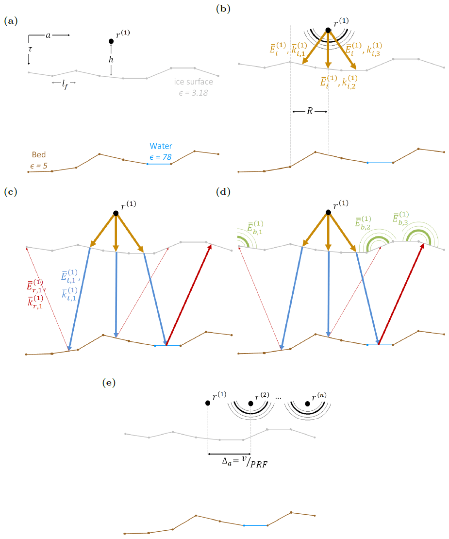
Figure 1Two-dimensional conceptual model of a RES simulation, defined in the direction of flight. (a) The material and geometric model for a radar observation. (b) The radar's spherical wavefront is approximated as rays directed at facets within a footprint beneath the aircraft. The simulator calculates a reflected and transmitted field strength based on the dielectric constant at the surface (ϵice). We do not show the surface reflection for simplicity. (c) The rays propagate through the ice, with a direction obeying Snell's Law. At the bed, reflected field strength and direction are controlled by dielectric contrast and incidence angle with the basal facet. (d) The backscattered electric field strength (Eb) is approximated with the Stratton–Chu integral. (e) The aircraft's position is incremented, and the process is repeated.
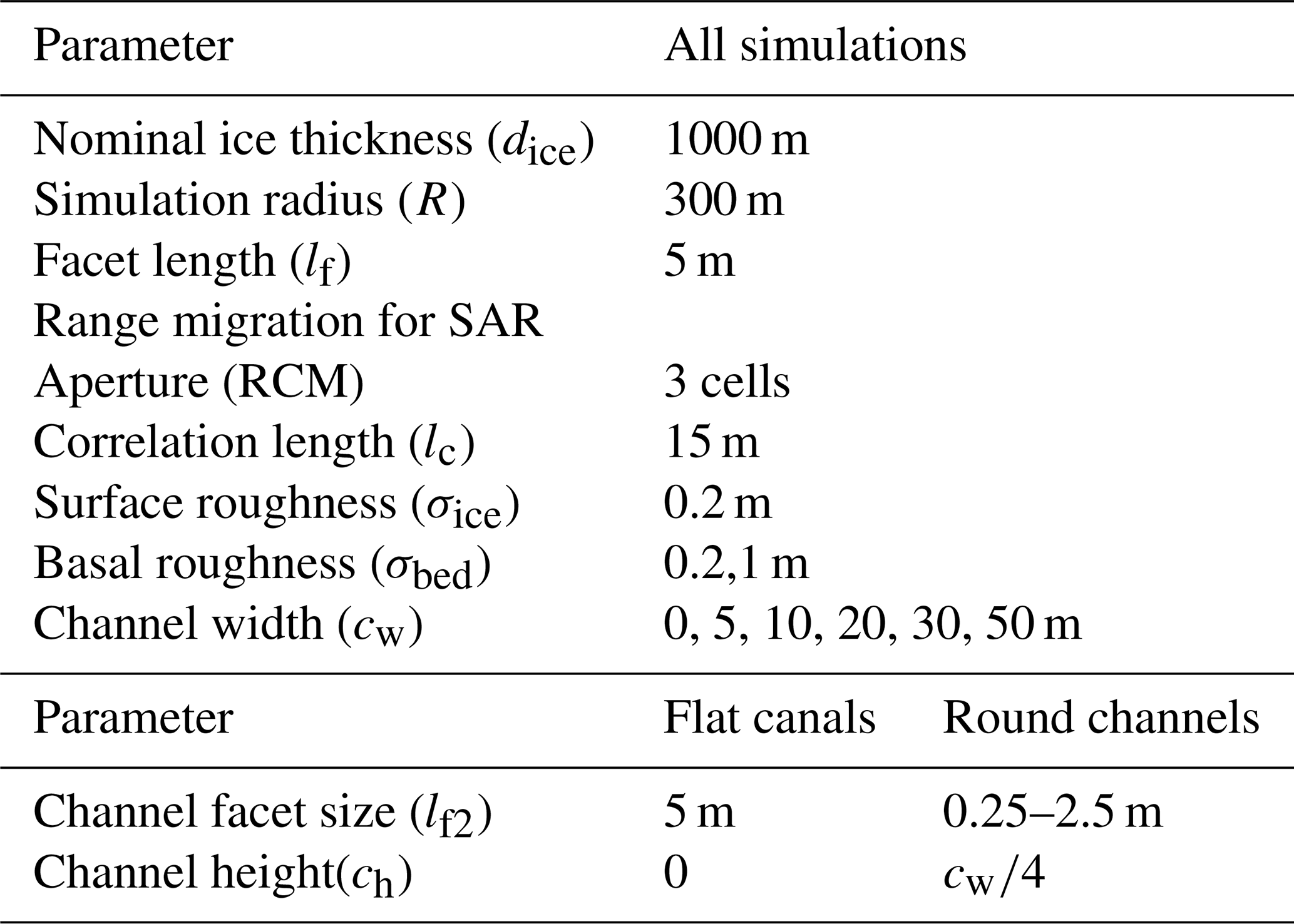
Figure 1 describes a generic conceptual model for a RES radar simulation. Parameters were chosen to emulate a typical helicopter-based airborne radar survey with the University of Texas Institute for Geophysics (UTIG) Multifrequency Airborne Radar Sounder with Full-phase Assessment (MARFA) instrument (Castelletti et al., 2017; Lindzey et al., 2020). An ice surface and a bed surface are defined in a three-dimensional Cartesian coordinate system, noted as Sice and Sbed, respectively. Figure 1a illustrates a 2-D representation of these surfaces, divided into N facets using a Delaunay triangulation algorithm, with characteristic length lf. The linear phase approximation (LPA) employed in Gerekos et al. (2018) allows the phase of the incident and reflected electric fields to vary linearly across each facet. LPA enables accurate simulations of coherent radar using relatively large facets (∼λ vs. with other methods). The facet size should be constrained according to Eq. (1), where h is the aircraft height and λ is the free-space radar wavelength (Gerekos et al., 2018). For simulations presented here, h=500 m and λ=5 m, consistent with a typical UTIG MARFA helicopter experiment. lf=5 m was chosen, consistent with Eq. (1).
The radar's spherical wavefront is simulated as a series of plane waves, with wavevectors and field strength vector directed at each ice surface facet within a radius R beneath the aircraft (Fig. 1b). A wider R will provide a more complete approximation of the radiated and returned electric field but comes at a computational cost proportional to R2. Therefore, R is chosen to balance these competing priorities, as we will discuss in detail.
Each ray's path is traced through transmission at Sice using Snell's Law, and then reflection is calculated from Sbed (Fig. 1c). In Fig. 1, the reflection from the ice surface is omitted for simplicity, since we are most concerned with reflections from the bed in this study. Reflected and transmitted field strengths ( and ) are calculated from the real component of the dielectric constant at Sice and Sbed, as discussed below. Attenuation loss between the surfaces is dependent on the complex component of the dielectric constant for ice (Gerekos et al., 2020), which is assumed constant over the short simulation distances presented here.
The total field at the radar antenna is then approximated as a summation of the backscattered electric fields () from individual propagated waves using the Stratton–Chu integral (Fig. 1d). A detailed treatment of the simulation mathematics is presented in Gerekos et al. (2018). Because of higher ice–water dielectric contrast, rays reflecting from a facet within Sbed identified as water will have higher amplitude than facets comprised of rock.
The radar pulse repetition frequency (PRF) and aircraft velocity v determine the spatial resolution between radar observations in the azimuth direction, Δa, as shown in Fig. 1e. In the field, the MARFA instrument employs a native pulse repetition frequency (PRF) of 6400 Hz and peak power of 8 kW, then these observations are coherently stacked in post processing to achieve along-track resolution of 1 m before focusing (Peters et al., 2007). We chose to simulate the final (stacked) PRF and power instead of the native parameters for computational efficiency.
Table 1Summary of RES simulation parameters. Parameters were chosen to replicate helicopter-based MARFA ice sounding experiments.
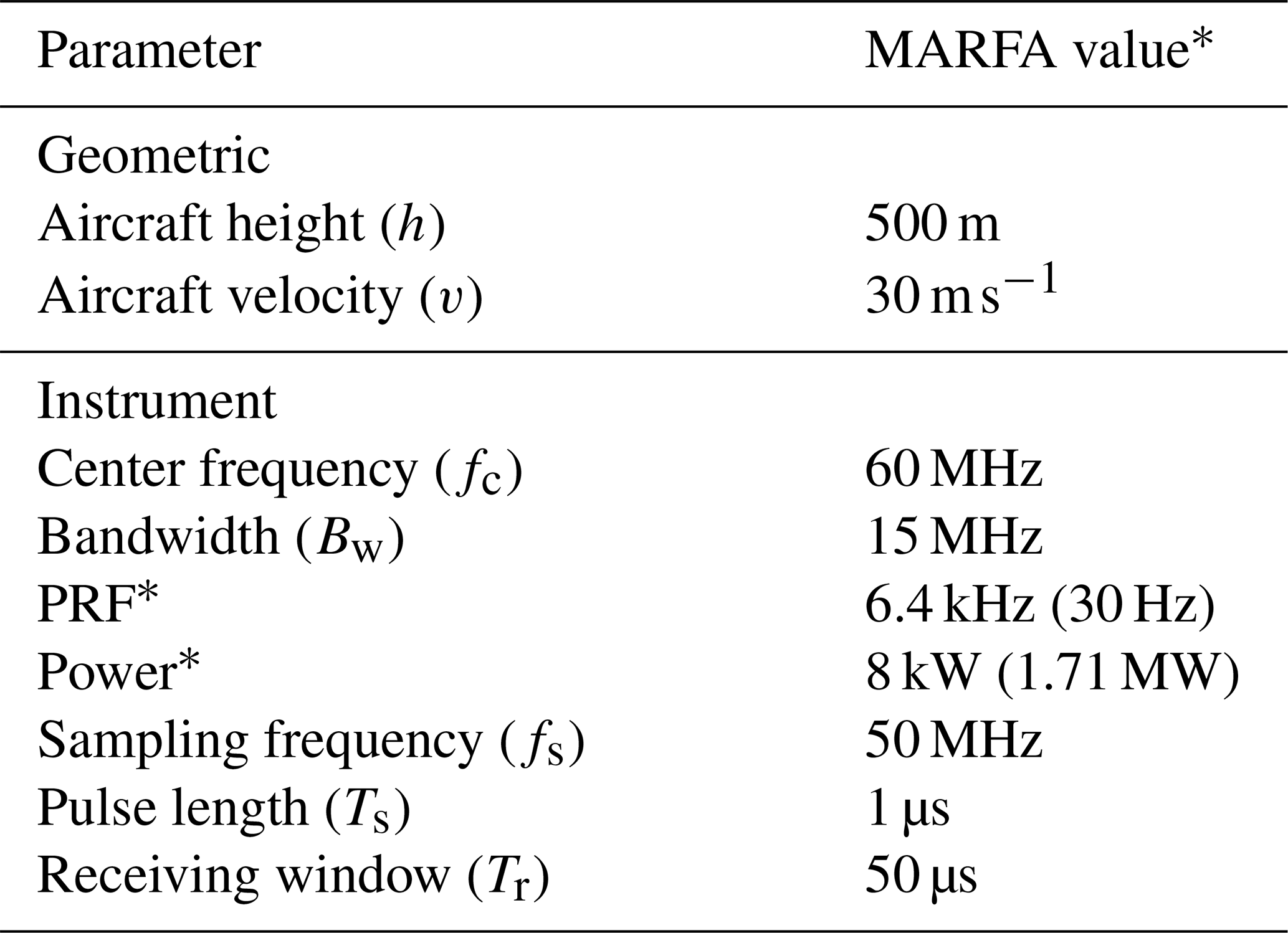
∗ For fields marked with an asterisk, the native MARFA radar value differs from the parameter used in the simulation. Simulation parameters are in parentheses and represent values after coherent pre-summing of raw MARFA data.
2.1 Dielectric material model
It is instructive to consider energy returned to the radar as the superposition of dielectric and geometric effects. Dielectric effects result from material property changes at an interface, while geometric effects result from the orientation of the interface's topography and the radar antenna. We will begin by discussing the implications of dielectric parameters then move on to geometric considerations.
A material model is applied to the simulation, where all facets on Sice and Sbed are assigned a complex dielectric constant, ϵ. The refractive index η for each material is derived from ϵ (Eq. 2). For simplicity, we have chosen a three-material model consisting of ice, rock, and water, with dielectric constants as presented in Table 2. Facets across Sice are assigned ϵice. Facets on Sbed are assigned ϵrock unless they are part of a water structure, which are assigned .
Table 2Complex dielectric constants for materials in radar simulations (Peters et al., 2005; Fujita et al., 2000; Midi et al., 2014; Glover, 2015). For each material, we chose a value within the range published in the literature. Further analysis of sensitivity to these material parameters is presented in the discussion.
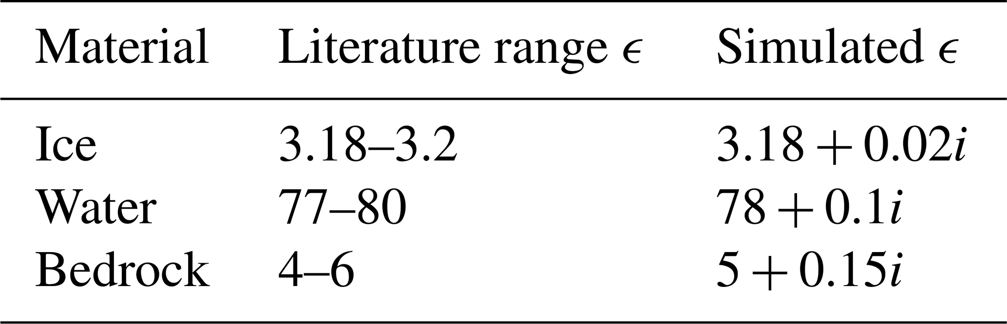
For a facet at nadir, absolute reflectivity Rabs results from the contrast between the refractive indices of ice and the bed material (ηice and ηrock, respectively). A horizontal facet assigned ϵrock will have a lower reflectivity than one assigned by about 15 dB (Eq. 2). Real RES instruments are rarely calibrated to measure absolute reflectivity, and thus changes in received power, corrected for ice attenuation loss and geometric scattering, are assumed proportional to relative changes in reflectivity at the bed (Rrel). This forms the basis for the widely accepted assumption that Rrel≥ 10–15 dB over surrounding reflections implies the presence of liquid water (e.g., Young et al., 2016; Peters et al., 2007; Rutishauser et al., 2022).
The simulations presented in this paper assume only the three materials described in Table 2, with well-defined boundaries between hydrological and bedrock features. In real-world sub-glacial environments, additional material heterogeneity such as clays or hydrated tills exist, in addition to ambiguity in hydrological boundaries. We address the implications of this relatively simplistic material model in Sect. 5.
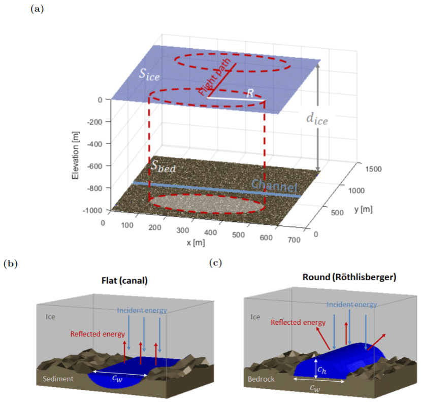
Figure 2Radar simulation geometry of the (a) flight path (red), aircraft or channel orientation, and simulation radius (R) across the model footprint. (b) A flat canal with width cw. (c) Geometry of a Röthlisberger or round channel with width cw.
2.2 Geometric model
We ultimately seek to develop the Stratton–Chu simulation method for constraining the extent and cross-sectional geometry of sub-glacial water features. Given this objective, it imperative to consider a menu of geometric constraints and how simulation parameters will emulate real-world RES returns from different targets. A basic simulation geometry for a hypothetical case is shown in Fig. 2a. These simulations consist of flat surfaces Sice at elevation 0 m and Sbed at −dice, where dice is the nominal ice thickness in m. The flight path is defined along the y direction, with the radar's dipole antenna oriented along the x direction. On the bed surface, a straight channel of width cw is oriented perpendicular to the flight path.
2.2.1 Surface roughness
Small-scale topography variation below the radar's detection limit, which we will refer to as roughness, can impact reflectivity by diffusely scattering incident radar energy. To account for this effect, random isotropic Gaussian variation is introduced to both Sice and Sbed via Eq. (3). lc is the correlation length in both the x and y directions. To capture scattering behavior due to topography changes at the radar wavelength scale, lc should be at least a few times the facet length lf, while remaining near λ. In our simulations, both lf and λ are ∼ 5 m, leading us to select lc = 15 m.
When we assume our surfaces are smooth relative to λ, we must add at least a negligible, non-zero roughness to avoid simulation artifacts, such as Bragg resonance (Gerekos et al., 2020). We always make these assumptions for Sice; therefore, σice = 0.2 m in all simulations presented here. We also use σbed = 0.2 m in “smooth” bed simulations.
Hubbard et al. (2000) measured topography of recently deglaciated bedrock at high resolution in the Swiss Alps. They showed variations near 1 m over horizontal distances of 15 m, which serves as our upper bound on σbed. We acknowledge this Alpine sub-glacial environment may differ considerably from common RES survey targets such as Thwaites Glacier in Antarctica. However, roughness studies from the Thwaites region integrate over long horizontal scales irrelevant to radar scattering (Bingham and Siegert, 2009; Hoffman et al., 2022). We proceed with the understanding that our range for σbed from 0.2 to 1 m may represent an imperfect but reasonable range of expected variation in small-scale topography.
2.2.2 Simulation radius
An appropriate choice of simulation radius R is vital to accurately simulate radar geometric scattering from the sub-glacial environment. R defines the radius of a vertical cylinder, bounding the simulation scope at each aircraft position increment. If R is sufficiently large to capture the entire antenna beam pattern cast on the bed surface, then the simulation will provide a complete representation of off-nadir clutter and target range migration. In many layered radar simulation experiments, R is chosen primarily to capture off-nadir clutter at the sub-surface target's apparent depth (Gerekos et al., 2018). Our experiments involve both a thick ice material layer and smooth Sice relative to λ, limiting the impact of off-nadir clutter. Therefore, we base our choice for R on two alternative criteria.
-
R must be greater than the pulse-limited radius Rpl at the glacier bed.
-
R captures adequate range migration to facilitate along-track focusing.
The first criterion assumes the majority of returned energy from a nadir-directed radar will come from within the pulse-limited footprint (Rpl) beneath the aircraft. Equation (4) approximates an upper limit on Rpl for a radar instrument with bandwidth Bw, where c is the speed of light in a vacuum. Actual Rpl will always be smaller than Eq. (4) predicts, due to refraction at the air–ice interface. For our simulations, with dice∼1000 m, Rpl≈ 130 m (Eq. 4). We consider this the minimum acceptable simulation radius, although clearly changes in aircraft height or simulated ice thickness will alter this limit.
An appropriate choice for R must also consider the desired range cell migration (RCM) at the bed surface. RCM is proportional to the change in physical distance a signal travels through air (rair) and ice (rice) to reach a target as the radar moves past (Eq. 5). In synthetic aperture radar (SAR) processing, an aperture length La is chosen with sufficient range cell migration to optimize along-track focusing. This process improves signal-to-noise ratio and along-track resolution (Cumming and Wong, 2005). In order to facilitate simulated data focusing, R must be greater than the aperture required for desired range migration. Selection of La and the focusing process is described at length in Sect. 2.3.
Our simulations target three cells of range migration at the bed surface (RCM(La)≥3). For dice = 1000 m and sampling frequency fs = 50 MHz, this translates to La = 277 m. All simulations presented here use R=300 m, meeting both the pulse-limited and range migration criteria. Real airborne RES focusing typically includes more range cell migration (RCM(La)=5 fast-time samples for MARFA); however, such a simulation radius would be computationally unrealistic. Therefore, our choice of R represents a compromise, and the implications will be discussed in Sect. 5. Simulations in thicker ice may require significantly larger R or further compromises in range migration.
2.2.3 Channel geometry
We seek to distinguish between two-channel geometries common to sub-glacial hydrology. A canal-like structure (Fig. 2b) will have a flat cross-section and produce a specular reflection. This type of feature is common when the surrounding bed is comprised of sediment or other soft material and the water pressure is high. Conversely, in a Röthlisberger channel (Fig. 2c), sub-glacial water carves a path through the ice above the bed surface (Röthlisberger, 1972). This type of channel is likely to form in areas where the substrate is impermeable bedrock with low water pressure (Walder and Fowler, 1994; Schroeder et al., 2013). We have confined ourselves to Röthlisberger channels and flat canals in this study as examples of common large-scale hydrological structures. Other known hydrologic features, such as Nye channels, may appear radiometrically similar to small canals, depending on their size and the radar wavelength. As algorithms and computational power enable higher-resolution models, additional sub-glacial structures are a logical extension of this work.
A Röthlisberger channel has an elliptical cross-section, with height ch in addition to channel width cw. We can infer from basic geometry that it will reflect radar energy divergently (Fig. 2c); therefore, the actual radar signature of a sub-glacial channel will be the superposition of its geometry and dielectric contrast. When representing the Röthlisberger curvature with flat facets, we must approximate the divergent scattering behavior by capturing reflections from multiple facets in the channel cross-section at nadir. In our simulations, we seek to capture reflections from at least the upper six facets within the simulation footprint as a reasonable estimate of Röthlisberger channel scattering (Fig. 3a).
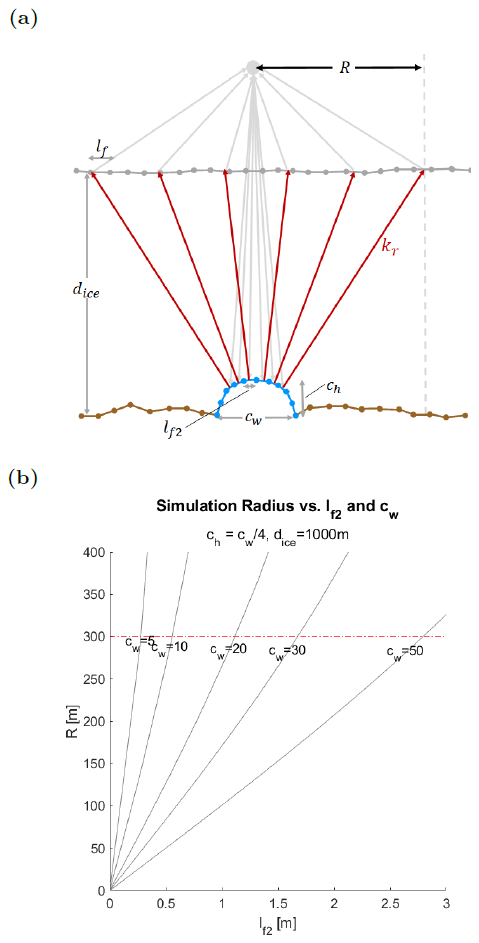
Figure 3(a) Schematic of simulation geometry for an elliptical cross-section of the Röthlisberger channel at nadir. A second, smaller facet length scale lf2 is introduced to facilitate accurate representation of curvature and divergent reflection character. (b) Relationship between R and lf2 is defined for a range of cw. We seek to limit R≤300 m for computational efficiency, imposing an upper limit on lf2 when simulating Röthlisberger channels
Given our desired range of cw and the constraint already imposed on R, it is clear that lf=5 m is too large to capture the scattering effect of a Röthlisberger channel. For our smallest channels (cw = 5 m), lf≤ 0.25 m is required to capture the desired facet reflections (Fig. 3b). Setting such a high resolution over all of Sice and Sbed is computationally unrealistic and negates many of the benefits of the Stratton–Chu simulation method (Gerekos et al., 2018). Therefore, we introduce a second facet length scale, lf2, which defines the facet length on Sice and Sbed only in a Röthlisberger channel location. lf2 has a maximum of , for dice = 1000 m and (Fig. 3b). When simulating flat canals, higher-resolution channel facets are unnecessary due to the specular nature of the reflection, and therefore lf2=lf.
2.3 Simulated data processing
The simulator outputs rangelines, which represent the electric field strength vs. fast-time τ returned from a single pulse, at azimuth time a. τ is discretized into range bins (index j) with increments of , where fs is the sampling frequency. The rangelines are compiled sequentially in azimuth, or slow time, into a 2-D raw radargram matrix (ξraw). Azimuth increments (index k) are equally spaced in time at .
The rangelines are then focused using a version of the range Doppler algorithm (RDA) (Cumming and Wong, 2005; Hélière et al., 2007). We first perform range compression by convolving each raw rangeline with the complex conjugate of the radar chirp, g(τ) over the radar receiving window Tr. The operation is performed by multiplication in the fast-time frequency domain.
We produce the focused radargram (ξf) by convolving the range-compressed radargram (ξRC) with a 1-D reference function (ϕ) in along-track blocks (Eq. 7). The block size, La, for each fast-time value of τ is chosen such that range migration equals three fast-time samples. Thus it is important to note that La increases with depth, and the simulation radius R must be greater than the maximum anticipated La.
A deeper discussion of mathematics and block processing required for along-track focusing is presented in Appendix A.
In all radargrams, we convert fast time to physical depth (d) and slow time to along-track distance (y) via Eqs. (8) and (9), where is the fast-time value for the surface reflection and PRF is the radar pulse repetition frequency.
The focused field in ξf is converted to power in decibels. We define along-track bed reflectivity in absolute terms (Rabs) by taking the maximum reflected power beneath the ice surface (Eq. 10a). Relative reflectivity (Rrel) compares Rabs to the mean reflectivity for a simulation with the same σbed and σice, but no channel is present (Rabs,0). Rrel therefore measures the relative reflectivity gain observed by the radar due to the channel's presence vs. surrounding frozen-bed material.
2.4 Hypothetical simulation cases
A basic simulation geometry is shown in Fig. 2. Our hypothetical simulation cases consisted of flat surfaces Sice and Sbed with elevations of 0 m and −1000 m, respectively. Each surface had isotropic Gaussian roughness as defined above. On the bed surface a single channel of width cw was oriented perpendicular to the flight path. Channel cross-sections were either flat canal-like structures (Fig. 2b) or round Röthlisberger channels with a channel height of (Fig. 2c).
A series of simulation experiments were run for both types of channels. Channel width and basal roughness were varied according to Table 3. Simulations involving flat canals used a single facet length of 5 m, while Röthlisberger channels necessitated a smaller lf2 in the channel location to accurately represent geometric scattering. Rangelines from each simulation were processed as described above, and along-track bed reflectivity from the focused radargram Rrel was compared for various scenarios.
Table 3Summary of RES simulation parameters for each channel geometry.
Basal roughness (σbed) impacted the absolute reflectivity of the solid bed material in our simulations (Rabs,0), which we use as a baseline for calculating the relative impact of channels on the radar echo (Eq. 10b). Simulations excluding liquid water, with σbed of 0.2 and 1 m, produced mean Rabs,0 equal to −107.9 ± 2.5 and −114.1 ± 2.4 dB, respectively.
Simulations of hypothetical Röthlisberger channels and flat canals with the same cw demonstrate the distinctly different radar signatures expected for the two geometries. Figure 4 shows along-track relative reflectivity for the two channel types, with cw = 20 m, compared to a frozen substrate with no liquid water. Flat canals have a distinct peak centered near the canal location, with maximum Rrel = 19.5 dB when σbed = 0.2 m and 22.9 dB when σbed = 1 m. Regardless of roughness, a 20 m flat canal influences the radar echo for a few hundred meters along track. The reduced gain of 3.4 dB for a canal surrounded by a smoother substrate is consistent with the higher absolute reflectivity of the surrounding surface as discussed above.
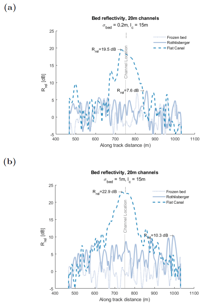
Figure 4Simulated along-track Rrel for 20 m channels compared to a dry substrate with (a) σbed=0.2 m and (b) σbed=1 m. All simulations had the same Gaussian roughness correlation length of lc=15 m.
When flowing through a rough bed (Fig. 4b), a 20 m simulated Röthlisberger channel increased along-track Rrel for more than 500 m. The maximum peak in Rrel for this channel is 10.3 dB, occurring when the channel is far from nadir. In our smoother bed simulations, the same 20 m Röthlisberger cross-section produced peak Rrel of only 7.6 dB (Fig. 4a), which could be nearly indistinguishable from fluctuations in reflectivity from the frozen substrate. Larger Röthlisberger channels produce only moderate gains in Rrel, with the largest (50 m) channels having peak Rrel = 13.2 dB (Fig. 5).
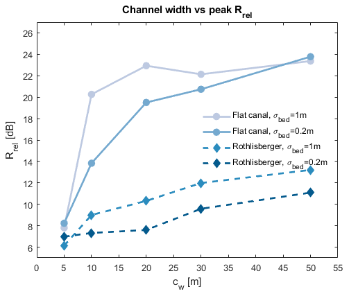
Figure 5Positive correlation between cw and Rrel for both Röthlisberger channels and flat canals. The increase in Rrel is much more pronounced for flat canals.
Figure 5 shows peak Rrel generally increases with width for both channels and canals, as an increasing proportion of the area within the radar's footprint contains liquid water. Flat canals exhibit a much stronger correlation between radar reflectivity response and cw than Röthlisberger channels when cw < 20 m. At cw > 20 m, Rrel for flat canals increases more gradually as it appears to reach an asymptote of ∼ 24 dB.
To demonstrate the simulator's utility in sub-glacial hypothesis testing, we compared simulated reflectivity to a single flight line collected with UTIG's 60 MHz MARFA instrument aboard an AS-350 B2 helicopter. The 16 km line (THW2/UBH0c/X243a) was part of an airborne radar survey of Thwaites Glacier conducted between 2020 and 2022. The helicopter was flown at a nominal height of 500 m above ground level with target velocity of 30 m s−1. Precise aircraft positioning and orientation were recorded with an onboard Renishaw laser altimeter, Trimble Net-R9 dual-frequency GNSS, and Novatel SPAN IGM-1A inertial navigation, as described in Lindzey et al. (2020).
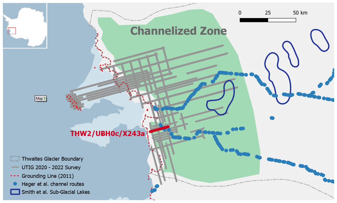
Figure 6The grounding line region of Thwaites Glacier, with the region of channelized hydrology proposed by Schroeder et al. (2013) highlighted. UTIG MARFA radar survey lines collected between 2020 and 2022 are shown in grey. Likely high volume channel routes suggested by Hager et al. (2022) are shown in blue, and the location of THW2/UBH0c/X243a is highlighted for reference.
4.1 Study area
Schroeder et al. (2013) first postulated a hydrological system dominated by channelized drainage within ∼ 45–70 km of the Thwaites grounding line (Fig. 6) based on data interpretation from the extensive 2003–2004 Airborne Geophysics of the Amundsen Sea Embayment, Antarctica (AGASEA) radar survey. The hypothesis was largely derived from observations of high local bed reflectivity, combined with anisotropy in the radar specularity content. Specularity content measures the relative diffuse or specular nature of radar returned power. Schroeder et al. (2013) postulated that extensive Röthlisberger channels could produce such radiometric signatures due to their geometric orientation.
Hager et al. (2022) ran a suite of sub-glacial hydrology simulations to evaluate the probability of persistent channelization routes beneath Thwaites. Their analysis concluded that Thwaites' near terminus hydrology is most likely comprised of a few persistent, high volume channels flowing toward the central grounding zone. Two probable routes were proposed, also shown in Fig. 6.
Although evidence for sub-glacial hydrology dominated by channelization in this region of Thwaites Glacier is strong, structures such as canals or lakes are not unprecedented. For example, Smith et al. (2017) identified a series of four active sub-glacial lakes that drained between June 2013 and January 2014. As seen in Fig. 6, at least one of these lakes is within the channelized region as defined in Schroeder et al. (2013).
Our chosen flight line, THW2/UBH0c/X243a, transects one of the proposed Hager et al. (2022) channel routes, and the radargram shows an isolated bright reflection coincident with this location, as shown in Fig. 7. Data from THW2/UBH0c/X243a were range compressed, corrected for geometric spreading loss and aircraft position, and focused in azimuth as described in Peters et al. (2007). This azimuth focusing is analogous to the procedure described in Sect. 2.3, although a longer aperture sufficient for range migration of five cells is used.
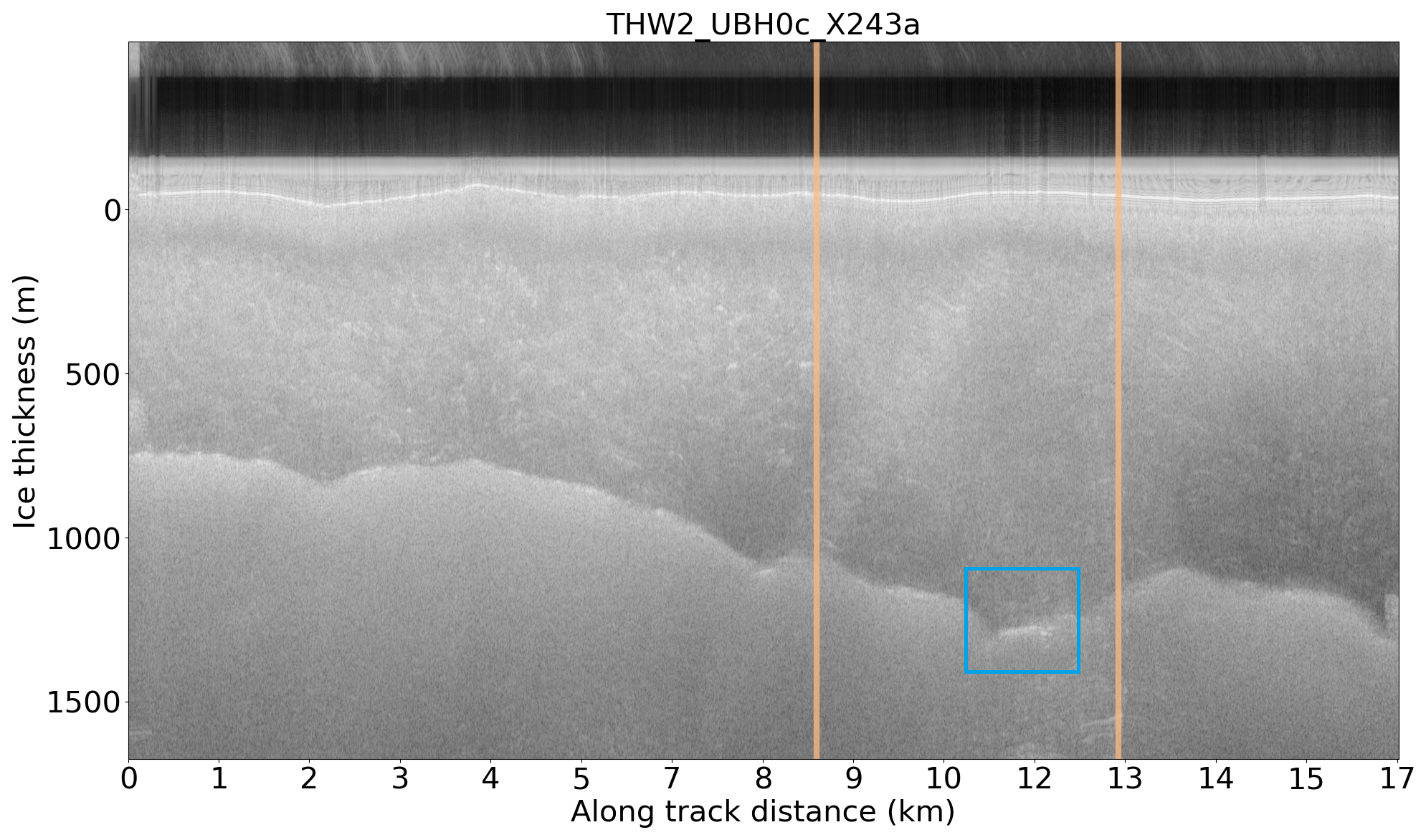
Figure 7Focused radargram for THW2/UBH0c/X243a. The bright bed reflection corresponding to the proposed channel location is boxed. Vertical lines represent the extent of the flight line reproduced in the simulations.
The along-track surface and bed profiles were picked from the radargram. One-way attenuation loss of 13.8 ± 1.4 dB km−1 was estimated using a spatially constrained linear regression model as outlined in Schroeder et al. (2016).
4.2 THW2/UBH0c/X243a simulation methodology
We simulated a 4 km segment of THW2/UBH0c/X243a containing the proposed channel, as depicted in Fig. 7. Along-track ice and surface elevations at nadir were calculated from the THW2/UBH0c/X243a focused radargram. From these data, we built elevation matrices for both the ice and bed surfaces (, ) which vary in y according to the respective radar profiles but have no x variation.
To build appropriate across-track (x) topography, separate 2-D topographic matrices were created from BedMachine V2 data (, ) (Morlighem, 2020a, b). The radar- and BedMachine-derived topography were superimposed to create simulation surfaces Sice and Sbed via Eq. (11), where w is a quadratic weighting function varying between 1 at the surface edges and 0 at nadir. Srough is an isotropic Gaussian surface, adding random roughness with σ = 0.2 m over correlation length lc = 15 m.
In an ice-penetrating RES survey, the aircraft attempts to “drape” the ice surface by flying at a constant height above ground level (500 m for UTIG helicopter based surveys). We simulate this with a polynomial interpolation of the radar-derived ice elevation along track, z0(y). For our simulations of THW2/UBH0c/X243a, z0 is a seventh-order polynomial, although in practice the polynomial order is somewhat subjective. The fitted function should approximate major terrain features in with gentle elevation changes, consistent with actual aircraft operation.
z0(y) is subtracted from Sice and Sbed, setting the average ice surface elevation to ∼ 0 m (Eq. 11). The simulated aircraft elevation h is a constant 500 m. This approach preserves known ice geometry at nadir, and minor topographic features appear as variations in aircraft range to target.
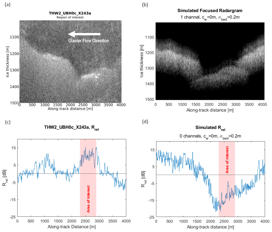
Figure 8(a) A 4 km region from actual THW2/UBH0c/X243a radargram containing the Hager et al. (2022) channel location. (b) Simulated THW2/UBH0c/X243a radargram with no water, σbed = 0.2 m. (c) Bed relative reflectivity from the actual THW2/UBH0c/X243a. The proposed channel location is highlighted in red as the area of interest. (d) Simulated THW2/UBH0c/X243a relative reflectivity with no water, σbed = 0.2 m. The along-track location corresponding to the area of interest is highlighted in red.
The dielectric material model was applied to Sice and Sbed as described previously. We ran individual simulations using the same surfaces, varying the width and geometry of across-track-oriented channels in the location identified in Hager et al. (2022). Relative bed reflectivity from each simulation result was compared to the actual relative reflectivity from the focused THW2/UBH0c/X243a radargram (Fig. 8c). The comparison between simulated and real data provides constraints on the extent and geometry of any real hydrological features at this location.
4.3 THW2/UBH0c/X243a simulation results
Figure 8 compares a 4 km segment from THW2/UBH0c/X243a RES data with a simulation containing no water and σbed = 0.2 m. There are two bright reflections in this section of the radargram (Fig. 8a). The first is centered around 1100 m along track with a maximum Rrel = 11.6 dB. The second is a broad area of high reflectivity between 2300–2900 m, with Rrel peaks ranging from 13 to 15 dB (Fig. 8c). This reflector coincides with the location of persistent Röthlisberger channelization proposed in Hager et al. (2022) and is the primary area of interest along THW2/UBH0c/X243a for this study.
The radargram from our frozen-bed simulation (Fig. 8b) captures the basic bed topography well, but along-track reflectivity is not always aligned with the real THW2/UBH0c/X243a radargram. Simulated reflectivity near 1100 m is consistent with the real data, indicating that this reflectivity peak could be the result of geometric effects from topography, rather than dielectric contrast from a water feature. However, for the region between 2300–2900 m, mean simulated Rrel is 22.8 dB below the value observed in the real THW2/UBH0c/X243a data (Fig. 11). In our material model, a gain of this magnitude could only be consistent with a change in dielectric properties from rock to liquid water. It is also unlikely to be a Röthlisberger channel, since we have demonstrated such geometry is not conducive to increased reflectivity of more than 13.2 dB for very large channels. We therefore propose that this basal reflector at 2300–2900 m along-track could represent a specular hydrological structure, such as a flat canal, of unknown dimensions.
When a single flat canal with cw = 20 m was added to the simulation, we observe a peak Rrel of 6.8 dB over a narrow 150 m range along track (Fig. 9). This reflectivity gain is consistent with our findings from hypothetical simulation cases described above. However, the gain in reflectivity and along-track extent are insufficient to match the reflectivity profile observed in the real THW2/UBH0c/X243a RES data (Figs. 9b and 8c). Therefore, we conclude that the reflector cannot be a narrow, isolated flat canal.
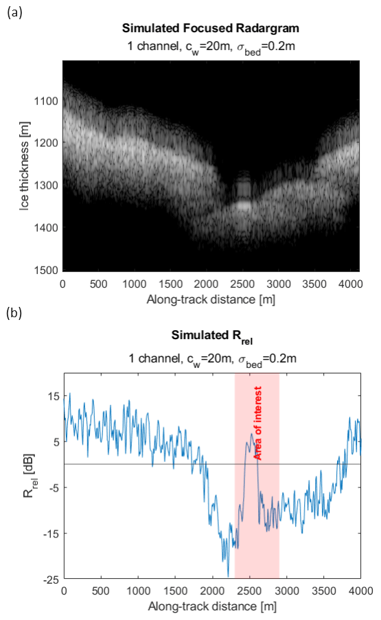
Figure 9(a) Simulated radargram with a single 20 m canal at the bed. (b) Relative reflectivity for simulation with 20 m canal at the bed.
The above results imply the reflector between 2300–2900 m may be a broader hydrological feature, such as an area with multiple flat canals. This hypothesis is compatible with the topographic context, given that it is in a low-lying area with steep topography just down-glacier. This is an ideal location for till and liquid water to accumulate if the ice exists at its pressure melting point.
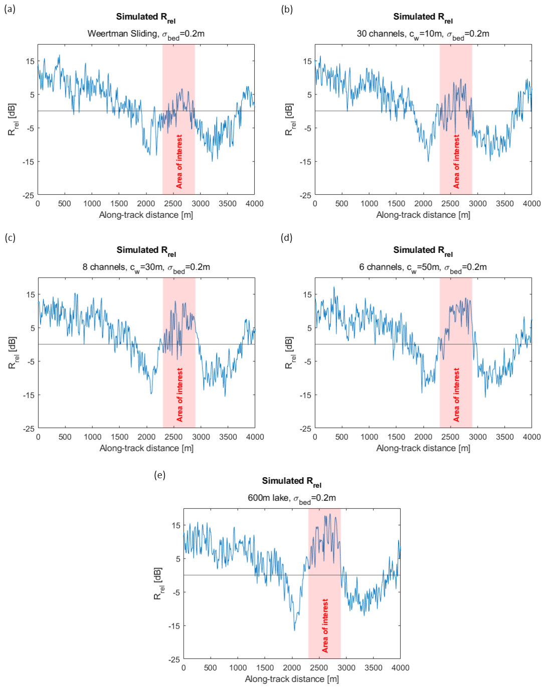
Figure 10Rrel for distributed hydrology simulations at 2300–2900 m along track. (a) A 600 m wet bed surface (Weertman sliding), (b) 30 flat canals with cw=10 m, (c) 8 flat canals with cw=30 m, (d) 6 flat canals with cw=50 m, and (e) the entire 600 m area covered with a flat, specular waterbody (e.g., sub-glacial lake).
Figure 11 compares the difference between THW2/UBH0c/X243a and simulated Rrel for five simulations of such hydrological features. We compare both the mean and peak difference in Rrel between 2300–2900 m and conclude that each more closely approximates THW2/UBH0c/X243a than our frozen bed or single 20 m channel simulation. First, we consider the glacier sliding condition originally proposed by Weertman (1964). In this scenario, a thin water film (perhaps a few centimeters thick) coats the basal interface. We model this by maintaining the basal topography with σbed = 0.2 m, but all facets from 2300 m 2900 m are assigned . This simulation has a broad increase in reflectivity in the area of interest (Fig. 10a); however, the mean Rrel between 2300–2900 m is 9.4 dB below the actual THW2/UBH0c/X243a value (Fig. 11).
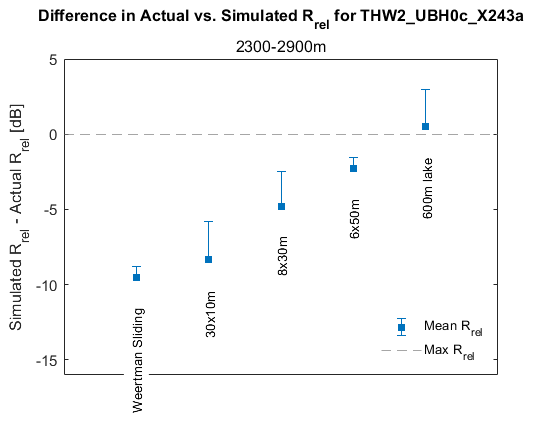
Figure 11Mean difference between actual and simulated Rrel over the area of interest at 2300–2900 m for all simulations of THW2/UBH0c/X243a. Positive error bars show the difference between mean and peak Rrel over 2300–2900 m.
Figure 10b shows simulated Rrel when 30 narrow, flat canals (cw = 10 m) were placed over the same 600 m region along track. This creates a region where 50 % of the area is covered with 10 m flat canals between areas of bed material with smooth basal roughness (σbed = 0.2 m). Mean Rrel at 2300–2900 m for this simulation is slightly higher than the Weertman film scenario in Fig. 10a but still 8.2 dB below the target Rrel from THW2/UBH0c/X243a.
The third simulation in Fig. 10c has eight larger flat canals (cw = 30 m) evenly spaced across the same 600 m region. This simulation has less water coverage than the 30 m × 10 m flat canal simulation (40 % vs. 50 %), yet the wider channels increased mean Rrel by 3.5 dB (Fig. 11). This result reinforces that the shape of hydrological feature, not just the extent, makes a significant difference to the resulting reflectivity profile. Mean Rrel for the 8 m × 30m simulation was 4.8 dB below actual values. When the geometry is changed to six canals of 50 m (Fig. 10d), mean Rrel improves to just 2.3 dB below THW2/UBH0c/X243a.
The final simulation includes a very broad area of specular (σbed = 0 m) water covering the bed between 2300–2900 m. Due to its size, we refer to this feature as the “600 m lake” in Figs. 10 and 11. Mean Rrel over 2300–2900 m for this simulation deviates by only 0.6 dB from the actual THW2/UBH0c/X243a data. However, this 600 m lake simulation includes several peaks as high as 18 dB, which is 3 dB higher than the maximum peaks observed in THW2/UBH0c/X243a. The maximum Rrel from both the 8 m × 30 m and 6 m × 50 m simulations more closely matched the peaks observed in THW2/UBH0c/X243a.
We infer our feature at 2300–2900 m could be a wide area of sub-glacial water. Of the scenarios we tested, simulated reflectivity was most consistent with canals averaging ∼ 30–50 m, with at least 50 % water coverage, or a sub-glacial lake. Although THW2/UBH0c/X243a and our simulations demonstrate similar reflectivity profiles, we have not explored a comprehensive range of bed materials or water geometries. In Sect. 5, we address these omissions and the resulting limitations.
Our comparison of Röthlisberger vs. flat canal reflectivity implies that a real world Röthlisberger channel, even one of significant size, may not exhibit an obvious reflectivity increase. Röthlisberger channels will scatter energy divergently (Fig. 2c); therefore, we see a smaller magnitude impact to Rrel over a greater distance than an equivalent flat canal. The simulator also demonstrates the radar's sensitivity to relatively narrow, flat canals. A single canal ∼ 10 m can exhibit a reflectivity peak > 15 dB (Fig. 5, nFlat canal). Such a hydrological feature would cover < 5 % of the radar's pulse-limited footprint under 1000 m of ice.
In our simulations of hypothetical cases, increasing σbed from 0.2 to 1 m reduced radar echo power by 6.2 dB. These results are intuitive. Scattering loss from a rougher surface will be larger and more variable, resulting in lower absolute reflectivity. Increasing roughness also alters the geometric contrast between the hydrological feature and surrounding material. The effect is most pronounced for flat canals with cw = 10–20 m. The impact of the bed roughness near flat canals diminishes as cw exceeds 30 m, when reflected energy from the water feature dominates the radar return.
Our examination of roughness in this study was deliberately limited, as the relationship between roughness and scattering is complex and dependent on correlation length lc. Bingham and Siegert (2009) and Peters et al. (2005) each calculated wide ranges in RES-derived roughness across Antarctica. Roughness in these studies was measured with lc > 1 km. Our method for building simulated ice and bed surfaces directly incorporates RES observations of topography with resolution lf = 5 m (see Sect. 4.2). Therefore, any relationship between scattering and large scale roughness, as defined in these previous studies, is captured explicitly in our simulations.
Smaller-scale sub-glacial roughness (lc < a few wavelengths) is more challenging to measure directly; therefore, actual values are poorly constrained. Our hypothetical case simulations demonstrate bed roughness over lc = 15 m may alter radar echoes without a change in dielectric properties. This is consistent with Peters et al. (2005), who calculated theoretical scattering loss due to roughness could exceed 20 dB when lc≪ first Fresnel zone. A comprehensive examination of basal roughness, incorporating a broad range of both lc and σbed, is possible with our simulation method. Such an investigation is an active area of interest for future work. Our limited current examination of roughness demonstrates that RES detection of sub-glacial water must be nuanced. Large changes in Rrel may constitute a liquid water signature but could also indicate spatial heterogeneity in roughness or substrate material.
Given the limited reflectivity response from Röthlisberger channels, more advanced analysis techniques may be required to detect and characterize them accurately. This could include examination of specularity content as described in Schroeder et al. (2015). Specularity content quantifies the diffuse or specular quality of radar reflections by comparing returned power over two different SAR apertures. Schroeder et al. (2013) argued that specularity content from Röthlisberger channels will be orientation dependent; high values are expected if the radar path is aligned along the channel, and lower values are expected if the path is transverse to it. By contrast, flat interfaces such as canals and lakes should exhibit high and isotropic specularity content. Although our simulation methodology produces a focused product, it requires a simulation radius R greater than the SAR aperture La. Current computational constraints limit our choice of R to well below the aperture length of 2 km recommended in Schroeder et al. (2015). Therefore, although simulating specularity content would be a valuable advance, we have left it to a future study.
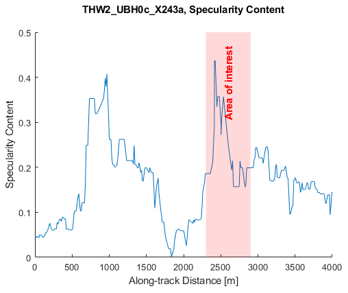
Our THW2/UBH0c/X243a simulations from Thwaites Glacier demonstrate the reflectivity magnitude may be consistent with a wide, flat water feature surrounded by bedrock. Although we did not simulate specularity content, we observe a prominent peak in actual specularity content from THW2/UBH0c/X243a (Fig. 12). This observation could support the hypothesis that the reflector at 2300–2900 m is a series of flat canals or a lake, since THW2/UBH0c/X243a is transverse to the channelized flow hypothesized in Hager et al. (2022) (Fig. 6). An orthogonally oriented radar transect could enable a more definitive diagnosis of the hydrological feature.
Further, while our flat canal or lake configurations appear likely, we cannot preclude all competing hypotheses without exploring many additional scenarios beyond the scope of this work. Other water geometries, such as Nye channels or water sheets (Creyts and Schoof, 2009), combined with a broader range of roughness length scales, could fit the original THW2/UBH0c/X243a reflectivity profile. Future work should identify computational or process efficiencies to allow comprehensive coverage of all possible simulation variables.
The material model in this study was also deliberately simple. Many possible bed materials exist, ranging from frozen bedrock to clays with real dielectric constants between 2.7–36 (Fig. 13) (Christianson et al., 2016; Tulaczyk and Foley, 2020; Peters et al., 2005). As we demonstrated in the frozen-bed simulation, the feature at 2300–2900 m requires an apparent reflectivity gain of 22.8 dB over the surrounding substrate. Roughness may contribute some of this difference; however, the observation is most consistent with a significant material transition. Figure 13 shows that the dielectric contrast between sub-glacial water and most clays or hydrated tills is less than 10 dB, making them unlikely bed materials. Conversely, substrates with the lowest dielectric constants are generally frozen, and they are therefore inconsistent with the presence of liquid water. These constraints limit the likely substrates to a narrow range of materials with ϵ∼ 5, including saturated bedrock or hydrated tills with low permittivity.
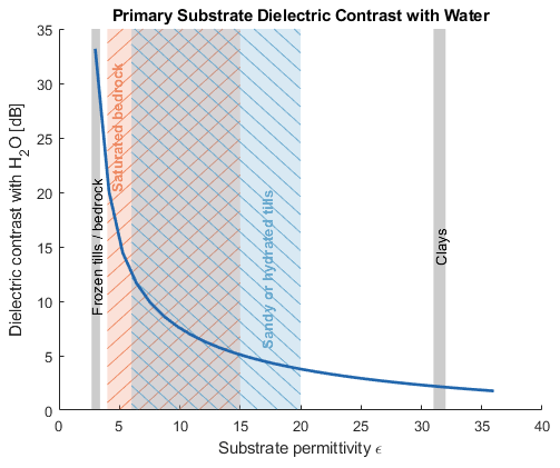
Figure 13Dielectric contrast between liquid water (ϵ=78) and substrates with permittivity from ϵ = 2.7–36. Example bed material permittivity ranges from Tulaczyk and Foley (2020) are provided as reference.
We also assumed constant radar attenuation in the ice. This assumption is reasonable given the short physical distances of our radar simulations. Simulations over greater distances may require introducing variation in the imaginary component of ϵice to account for heterogeneous attenuation loss.
Several notable inconsistencies between our best simulations and the original THW2/UBH0c/X243a data remain. First, Rrel over the beginning and final 500 m of all the simulations are about ∼ 5–8 dB higher than the THW2/UBH0c/X243a RES data. This may indicate a change in σbed near the edges of the simulated region. The low-lying area in the region is a perfect topographical feature to accumulate sediments, which likely have low roughness. The steeper and elevated topography near the edges of the simulated region may be exposed bedrock, with greater roughness, which we have shown in our hypothetical case simulations can reduce Rrel. In future iterations of the simulator, we would enable heterogeneity in σbed in order to capture this type of variation explicitly.
Rrel near 2000 m along track in all simulations was ∼ 10 dB lower than actual reflectivity from THW2/UBH0c/X243a (Fig. 10). This is coincident with a steep topographical feature in the THW2/UBH0c/X243a radargram. Steep slopes such as this likely represent a limitation of our simulation approach. The surface representation using 5 m flat facets will inherently direct more reflected energy away from the antenna position than a real surface. Therefore, caution is imperative when interpreting results near steep topography.
There are several additional limitations of our simulation method for testing sub-glacial hypotheses. The simulation radius of R = 300 m explicitly limits the impact of range migration and clutter. A more complete simulation incorporating a larger R would be beneficial to simulations in thicker ice or focusing over longer apertures. Future work should combine additional computing power with simulated facet roughness (Gerekos et al., 2023) for additional realism and efficiency.
Our three-dimensional model for topography was derived from a single along-track RES flight line, which enables high confidence and sufficient resolution for ice geometry at nadir. However, this has the obvious limitation of requiring a previous flight line to build our simulation. We lack similar observation density across-track, leaving low-resolution (500 m) open-source DEMs (such as BedMachine V2 (Morlighem, 2020a, b)) as our best option for approximating off-nadir features. This asymmetry is not problematic for replicating basic topography at nadir, but the lack of realistic off-nadir features reduces the sharpness of the focusing algorithm. We can see this effect by comparing the image quality in Fig. 8a to simulated results in Fig. 8b or Fig. 9a. This limitation also clearly reduces our ability to assess hypotheses involving any off-nadir targets.
It is also important to note that the simulation in Fig. 8d exhibits along-track Rrel variation > 30 dB without any change in dielectric properties at the bed. This demonstrates that significant changes in bed echo strength are possible due to topography alone. When inferring the presence of sub-glacial hydrological features from RES data, care must be taken to consider reflectivity within the context of bed topography, hydraulic potential, attenuation, and other factors that may influence the radar echo strength. This observation also demonstrates the value of our simulation methodology for confirming the presence and extent of sub-glacial water.
In the exercise presented here, we optimized a radar simulation technique developed by Gerekos et al. (2018) to study the theoretical RES response from sub-glacial systems. The simulator incorporates the Stratton–Chu integral and linear phase approximation to efficiently estimate backscattered radar signal from simulated targets. Through a series of hypothetical simulation cases, we demonstrated the impact on relative reflectivity from rounded Röthlisberger channels or specular flat canals surrounded by bed materials of varying roughness. These simulations confirmed that reflectivity is highly dependent on both the size and cross-sectional shape of the sub-glacial water structure. Our results can be applied broadly to infer the presence, size, and structure of sub-glacial waterbodies from RES surveys in a more robust and sophisticated way than previous methods.
In our example flight line THW2/UBH0c/X243a from Thwaites Glacier, we demonstrated the simulator's utility in testing relevant hypotheses in sub-glacial hydrology. A large water structure could produce the elevated reflectivity beneath Thwaites Glacier, in a region coinciding with a channel route proposed by Hager et al. (2022). Of the scenarios we tested, the radar signature was most consistent with canals averaging > 30 m and covering at least half the area for 600 m along track. Additional simulations including a broader range of hydrological structures and bed materials may be useful to conclusively characterize the feature. Further, although we do not see a Röthlisberger channel at this precise location, our findings do not preclude Röthlisberger channelization further upglacier. Simulations of new and existing RES survey data across the Thwaites catchment could characterize the extent of upglacier channelization.
The method we outline has broad applicability for studying the basal environment of large glaciers. As we have shown, the simulation methodology can offer useful constraints when testing sub-glacial hypotheses. Scientific intuition, additional data inputs, and more computational power will improve the promise of this technique. Future work may include additional computational efficiency to enable more extensive simulations, as well as comprehensive investigations on the impact of substrate roughness, material properties, and additional water geometries.
RES data collection is logistically challenging and expensive. A forward model capable of predicting optimal locations for sub-glacial survey targets, instead of modeling existing flight lines, is an area of interest for future work. In such a forward model, computing resources must be optimized by strategically constraining parameter sets, and performing sensitivity tests for many of the variables considered here.
We produce the focused radargram (ξf) by processing in along-track blocks. For a given fast-time range bin τj, the block size, La, is chosen such that range migration for a target equals three fast-time samples, as depicted in Fig. A1. Thus, it is important to note that the block size increases with depth, and the simulation radius R must be greater than the maximum anticipated La.
To process a block centered at slow-time a0, with depth τj, we begin with a block of length 2La from the range-compressed radargram (ξRC) as shown in Fig. A1. We calculated a 1-D reference function (ϕ), representing the Doppler phase modulation as the antenna travels across the aperture in slow-time a (Eq. A1) Peters et al. (2007); Legarsky et al. (2001); Hélière et al. (2007). The amplitude term, b, in Eq. (A1) is used in real-world RES processing to account for along-track variations in instrument gain and aircraft motion and to attenuate high Doppler frequency contributions at long apertures Legarsky et al. (2001); Peters et al. (2007). Our simulations do not contend with non-ideal flight or instrumentation variables, and we therefore use a simple Hamming window of width La for suppression of higher-frequency sidelobes.
The data block and reference function are Fourier transformed and convolved in the frequency domain (Fig. A2). The result is transformed back to the slow-time domain via inverse Fourier transform. Because the reference function ϕ is tuned at the center of the original block, the middle of the final block is better focused than the edges Hélière et al. (2007). For this reason, only half of the final block (length La) is written to the focused radargram ξf (Fig. A1). This process is repeated for each along-track block at all fast-time range bins until a complete focused radargram, ξf, is formed.
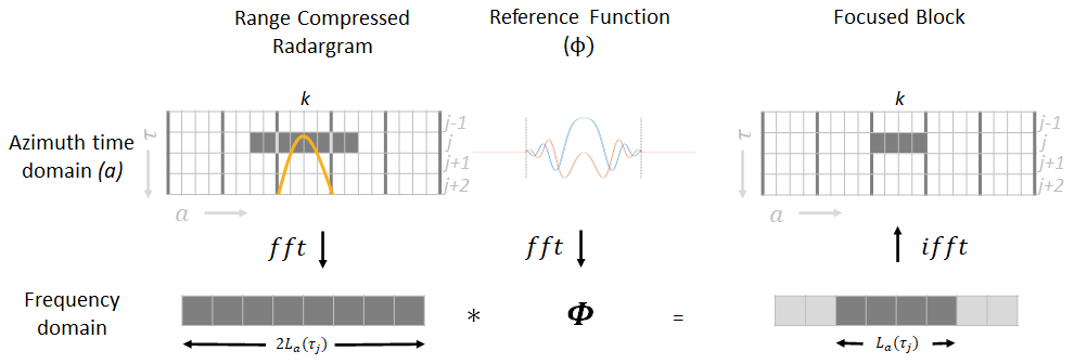
Figure A1Schematic representation of along-track (azimuth) focusing for a single block at discrete fast-time increment τj and azimuth block k in a simulated radargram. The orange hyperbola superimposed on the range-compressed radargram illustrates the theoretical range migration of a target with shortest fast-time range τj. We select an aperture length La such that range migration spans three sample cells (τj, τj+1, and τj+2).
All referenced data in this paper are made available at https://doi.org/10.5281/zenodo.8165256 (Pierce et al., 2023).
CP prepared the original draft, wrote modifications to the simulator, led the design and execution of experiments, and participated in the fieldwork to collect IPR data from Thwaites Glacier. CG contributed the original simulator software, assisted in experimental design and model validation, and provided significant editorial support. MS provided oversight and partial funding, as well as significant editorial contributions. LB provided important context for the project conceptualization, made significant editorial contributions, and led the field team responsible for IPR data collection over Thwaites Glacier. DB provided leadership support, funding, and programmatic resources for the investigation and IPR data collection over Thwaites Glacier. WSL provided funding and logistics support for the Thwaites IPR data collection, as well as editorial contributions. EA provided significant editorial review and advisory support. CKL made a significant contribution to planning and execution of the Thwaites Glacier IPR survey, provided input on the simulation experimental design, and provided editorial support. JS participated in the collection and validation of IPR data from Thwaites Glacier.
The contact author has declared that none of the authors has any competing interests.
Publisher's note: Copernicus Publications remains neutral with regard to jurisdictional claims made in the text, published maps, institutional affiliations, or any other geographical representation in this paper. While Copernicus Publications makes every effort to include appropriate place names, the final responsibility lies with the authors.
KIMST and Canadian Helicopters Limited (CHL) provided logistics, equipment, and personnel supporting RES data collection over Thwaites Glacier. Computational efforts were performed on the Tempest High Performance Computing System, operated and supported by University Information Technology Research Cyberinfrastructure at Montana State University. We would like to acknowledge individual contributions from Dillon Buhl, Greg Nguyen, and Kirk Scanlan. Their expertise was invaluable. Finally, we appreciate the insights provided by two anonymous reviewers. Their helpful comments significantly improved the quality of this paper.
This research was supported by the National Aeronautics and Space Administration (award no. 80NSSC20K1134), the Korea Institute of Marine Science & Technology Promotion (KIMST) funded by the Ministry of Oceans and Fisheries (RS-2023-00256677), the G. Unger Vetlesen Foundation, and the Montana State University Office for Research and Economic Development.
This paper was edited by Vishnu Nandan and reviewed by two anonymous referees.
Bingham, R. G. and Siegert, M. J.: Quantifying subglacial bed roughness in Antarctica: implications for ice-sheet dynamics and history, Quaternary Sci. Rev., 28, 223–236, https://doi.org/10.1016/j.quascirev.2008.10.014, 2009. a, b
Brinkerhoff, D., Aschwanden, A., and Fahnestock, M.: Constraining subglacial processes from surface velocity observations using surrogate-based Bayesian inference, J. Glaciol., 67, 385–403, https://doi.org/10.1017/jog.2020.112, 2021. a
Castelletti, D., Schroeder, D. M., Hensley, S., Grima, C., Ng, G., Young, D., Gim, Y., Bruzzone, L., Moussessian, A., and Blankenship, D. D.: An Interferometric Approach to Cross-Track Clutter Detection in Two-Channel VHF Radar Sounders, IEEE T. Geosci. Remote, 55, 6128–6140, https://doi.org/10.1109/TGRS.2017.2721433, 2017. a
Christianson, K., Jacobel, R. W., Horgan, H. J., Alley, R. B., Anandakrishnan, S., Holland, D. M., and DallaSanta, K. J.: Basal conditions at the grounding zone of Whillans Ice Stream, West Antarctica, from ice-penetrating radar, J. Geophys. Res.-Earth, 121, 1954–1983, https://doi.org/10.1002/2015JF003806, 2016. a
Chu, W., Schroeder, D. M., Seroussi, H., Creyts, T. T., Palmer, S. J., and Bell, R. E.: Extensive winter subglacial water storage beneath the Greenland Ice Sheet, Geophys. Res. Lett., 43, 12,484–12,492, https://doi.org/10.1002/2016GL071538, 2016. a
Creyts, T. T. and Schoof, C. G.: Drainage through subglacial water sheets, J. Geophys. Res.-Earth, 114, 1–18, https://doi.org/10.1029/2008JF001215, 2009. a
Cumming, I. and Wong, F.: Digital Processing of Synthetic Aperture Radar: Algorithms and Implementation, Artech House, Norwood, MA, 2005. a, b
Dunse, T., Schellenberger, T., Hagen, J. O., Kääb, A., Schuler, T. V., and Reijmer, C. H.: Glacier-surge mechanisms promoted by a hydro-thermodynamic feedback to summer melt, The Cryosphere, 9, 197–215, https://doi.org/10.5194/tc-9-197-2015, 2015. a
Fujita, S., Matsuoka, T., Ishida, T., Matsuoka, K., and Mae, S.: A summary of the complex dielectric permittivity of ice in the megahertz range and its applications for radar sounding of polar ice sheets, in: Physics of Ice Core Records, edited by: Hondoh, T., Hokkaido University Press, Sapporo, 185–212, http://hdl.handle.net/2115/32469, 2000. a
Gerekos, C., Tamponi, A., Carrer, L., Castelletti, D., Santoni, M., and Bruzzone, L.: A coherent multilayer simulator of radargrams acquired by radar sounder instruments, IEEE T. Geosci. Remote, 56, 7388–7404, https://doi.org/10.1109/TGRS.2018.2851020, 2018. a, b, c, d, e, f, g, h, i
Gerekos, C., Bruzzone, L., and Imai, M.: A Coherent Method for Simulating Active and Passive Radar Sounding of the Jovian Icy Moons, IEEE T. Geosci. Remote, 58, 2250–2265, https://doi.org/10.1109/TGRS.2019.2945079, 2020. a, b
Gerekos, C., Haynes, M. S., Schroeder, D. M., and Blankenship, D. D.: The Phase Response of a Rough Rectangular Facet for Radar Sounder Simulations of Both Coherent and Incoherent Scattering, Radio Sci., 58, 1–30, https://doi.org/10.1029/2022RS007594, 2023. a
Gilbert, A., Gimbert, F., Thøgersen, K., Schuler, T. V., and Kääb, A.: A Consistent Framework for Coupling Basal Friction With Subglacial Hydrology on Hard-Bedded Glaciers, Geophys. Res. Lett., 49, 1–10, https://doi.org/10.1029/2021GL097507, 2022. a
Glover, P. W. J.: 11.04 – Geophysical Properties of the Near Surface Earth: Electrical Properties, in: Treatise on Geophysics, second edition edn., edited by: Schubert, G., Elsevier, Oxford, https://doi.org/10.1016/B978-0-444-53802-4.00189-5, pp. 89–137, 2015. a
Hager, A. O., Hoffman, M. J., Price, S. F., and Schroeder, D. M.: Persistent, extensive channelized drainage modeled beneath Thwaites Glacier, West Antarctica, The Cryosphere, 16, 3575–3599, https://doi.org/10.5194/tc-16-3575-2022, 2022. a, b, c, d, e, f, g, h
Hélière, F., Lin, C. C., Corr, H., and Vaughan, D.: Radio echo sounding of Pine Island Glacier, West Antarctica: Aperture synthesis processing and analysis of feasibility from space, IEEE T. Geosci. Remote, 45, 2573–2582, https://doi.org/10.1109/TGRS.2007.897433, 2007. a, b, c
Hoffman, A. O., Christianson, K., Holschuh, N., Case, E., Kingslake, J., and Arthern, R.: The Impact of Basal Roughness on Inland Thwaites Glacier Sliding, Geophys. Res. Lett., 49, 1–11, https://doi.org/10.1029/2021GL096564, 2022. a
Hoffman, M. J., Andrews, L. C., Price, S. A., Catania, G. A., Neumann, T. A., Lüthi, M. P., Gulley, J., Ryser, C., Hawley, R. L., and Morriss, B.: Greenland subglacial drainage evolution regulated by weakly connected regions of the bed, Nat. Commun., 7, 13903, https://doi.org/10.1038/ncomms13903, 2016. a, b
Hubbard, B., Siegert, M. J., and Mccarroll, D.: Spectral roughness of glaciated bedrock geomorphic surfaces: Implications for glacier sliding, J. Geophysi. Res., 105, 21295–21303, 2000. a
Legarsky, J. J., Gogineni, S. P., and Akins, T. L.: Focused synthetic aperture radar processing of ice-sounder data collected over the Greenland ice sheet, IEEE T. Geosci. Remote, 39, 2109–2117, https://doi.org/10.1109/36.957274, 2001. a, b
Lindzey, L. E., Beem, L. H., Young, D. A., Quartini, E., Blankenship, D. D., Lee, C.-K., Lee, W. S., Lee, J. I., and Lee, J.: Aerogeophysical characterization of an active subglacial lake system in the David Glacier catchment, Antarctica, The Cryosphere, 14, 2217–2233, https://doi.org/10.5194/tc-14-2217-2020, 2020. a, b
Midi, N. S., Sasaki, K., Ohyama, R.-i., and Shinyashiki, N.: Broadband complex dielectric constants of water and sodium chloride aqueous solutions with different DC conductivities, IEEJ T. Electr. Electr., 9, S8–S12, https://doi.org/10.1002/tee.22036, 2014. a
Morlighem, M.: MEaSUREs BedMachine Antarctica, Version 2, NASA National Snow and Ice Data Center Distributed Active Archive Center [data set], https://doi.org/10.5067/E1QL9HFQ7A8M, 2020a. a, b
Morlighem, M., Rignot, E., Binder, T., et al.: Deep glacial troughs and stabilizing ridges unveiled beneath the margins of the Antarctic ice sheet, Nat. Geosci., 13, 132–137, https://doi.org/10.1038/s41561-019-0510-8, 2020b. a, b
Peters, M. E., Blankenship, D. D., and Morse, D. L.: Analysis techniques for coherent airborne radar sounding: Application to West Antarctic ice streams, J. Geophys. Res.-Sol. Ea., 110, 1–17, https://doi.org/10.1029/2004JB003222, 2005. a, b, c, d, e, f
Peters, M. E., Blankenship, D. D., Carter, S. P., Kempf, S. D., Young, D. A., and Holt, J. W.: Along-track focusing of airborne radar sounding data from west antarctica for improving basal reflection analysis and layer detection, IEEE T. Geosci. Remote, 45, 2725–2736, https://doi.org/10.1109/TGRS.2007.897416, 2007. a, b, c, d, e
Pierce, C., Gerekos, C., Skidmore, M., Beem, L., Blankenship, D., Lee, W. S., Adams, E., Lee, C.-K., and Stutz, J.: Supporting Data: Characterizing Sub-Glacial Hydrology Using Radar Simulations (Version 2), Zenodo [data set], https://doi.org/10.5281/zenodo.8165343, 2023. a
Priscu, J. C., Kalin, J., Winans, J., Campbell, T., Siegfried, M. R., Skidmore, M., Dore, J. E., Leventer, A., Harwood, D. M., Duling, D., Zook, R., Burnett, J., Gibson, D., Krula, E., Mironov, A., McManis, J., Roberts, G., Rosenheim, B. E., Christner, B. C., Kasic, K., Fricker, H. A., Lyons, W. B., Barker, J., Bowling, M., Collins, B., Davis, C., Gagnon, A., Gardner, C., Gustafson, C., Kim, O. S., Li, W., Michaud, A., Patterson, M. O., Tranter, M., Venturelli, R., Vick-Majors, T., and Elsworth, C.: Scientific access into Mercer Subglacial Lake: Scientific objectives, drilling operations and initial observations, Ann. Glaciol., 62, 340–352, https://doi.org/10.1017/aog.2021.10, 2021. a
Röthlisberger, H.: Water Pressure in Intra- and Subglacial Channels, J. Glaciol., 11, 177–203, https://doi.org/10.3189/s0022143000022188, 1972. a
Russo, F., Cutigni, M., Orosei, R., Taddei, C., Seu, R., Biccari, D., Giacomoni, E., Fuga, O., and Flamini, E.: An Incoherent Simulator for the Sharad Experiment, 2008 IEEE Radar Conference, RADAR 2008, Sheraton Golf Parco dei Medici, Rome, Italy, 26–30 May 2008, https://doi.org/10.1109/RADAR.2008.4720761, 2008. a
Rutishauser, A., Blankenship, D. D., Sharp, M., Skidmore, M. L., Greenbaum, J. S., Grima, C., Schroeder, D. M., Dowdeswell, J. A., and Young, D. A.: Discovery of a hypersaline subglacial lake complex beneath Devon Ice Cap, Canadian Arctic, Science Advances, 4, 1–7, https://doi.org/10.1126/sciadv.aar4353, 2018. a
Rutishauser, A., Blankenship, D. D., Young, D. A., Wolfenbarger, N. S., Beem, L. H., Skidmore, M. L., Dubnick, A., and Criscitiello, A. S.: Radar sounding survey over Devon Ice Cap indicates the potential for a diverse hypersaline subglacial hydrological environment, The Cryosphere, 16, 379–395, https://doi.org/10.5194/tc-16-379-2022, 2022. a
Schroeder, D. M., Blankenship, D. D., and Young, D. A.: Evidence for a water system transition beneath thwaites glacier, West Antarctica, P. Natl. Acad. Sci. USA, 110, 12225–12228, https://doi.org/10.1073/pnas.1302828110, 2013. a, b, c, d, e, f, g, h, i, j
Schroeder, D. M., Blankenship, D. D., Raney, R. K., and Grima, C.: Estimating subglacial water geometry using radar bed echo specularity: Application to Thwaites Glacier, West Antarctica, IEEE Geosci. Remote S., 12, 443–447, https://doi.org/10.1109/LGRS.2014.2337878, 2015. a, b, c
Schroeder, D. M., Seroussi, H., Chu, W., and Young, D. A.: Adaptively constraining radar attenuation and temperature across the Thwaites Glacier catchment using bed echoes, J. Glaciol., 62, 1075–1082, https://doi.org/10.1017/jog.2016.100, 2016. a
Smith, B. E., Gourmelen, N., Huth, A., and Joughin, I.: Connected subglacial lake drainage beneath Thwaites Glacier, West Antarctica, The Cryosphere, 11, 451–467, https://doi.org/10.5194/tc-11-451-2017, 2017. a
Spagnuolo, M. G., Grings, F., Perna, P., Franco, M., Karszenbaum, H., and Ramos, V. A.: Multilayer simulations for accurate geological interpretations of SHARAD radargrams, Planet. Space Sci., 59, 1222–1230, https://doi.org/10.1016/j.pss.2010.10.013, 2011. a
Tulaczyk, S. M. and Foley, N. T.: The role of electrical conductivity in radar wave reflection from glacier beds, The Cryosphere, 14, 4495–4506, https://doi.org/10.5194/tc-14-4495-2020, 2020. a, b
Walder, J. S. and Fowler, A.: Channelized subglacial drainage over a deformable bed, J. Glaciol., 40, 3–15, https://doi.org/10.1017/S0022143000003750, 1994. a
Weertman, J.: The Theory of Glacier Sliding, J. Glaciol., 5, 287–303, https://doi.org/10.3189/s0022143000029038, 1964. a
Wright, A. P., Young, D. A., Roberts, J. L., Schroeder, D. M., Bamber, J. L., Dowdeswell, J. A., Young, N. W., Le Brocq, A. M., Warner, R. C., Payne, A. J., Blankenship, D. D., Van Ommen, T. D., and Siegert, M. J.: Evidence of a hydrological connection between the ice divide and ice sheet margin in the Aurora Subglacial Basin, East Antarctica, J. Geophys. Res.-Earth, 117, 1–15, https://doi.org/10.1029/2011JF002066, 2012. a
Young, D. A., Schroeder, D. M., Blankenship, D. D., Kempf, S. D., and Quartini, E.: The distribution of basal water between Antarctic subglacial lakes from radar sounding, Philos. T. R. Soc. A, 374, 20140297, https://doi.org/10.1098/rsta.2014.0297, 2016. a, b, c
- Abstract
- Introduction
- Simulation methodology
- Results – hypothetical simulation cases
- Application to Thwaites Glacier
- Discussion
- Conclusions
- Appendix A: Along-track focusing
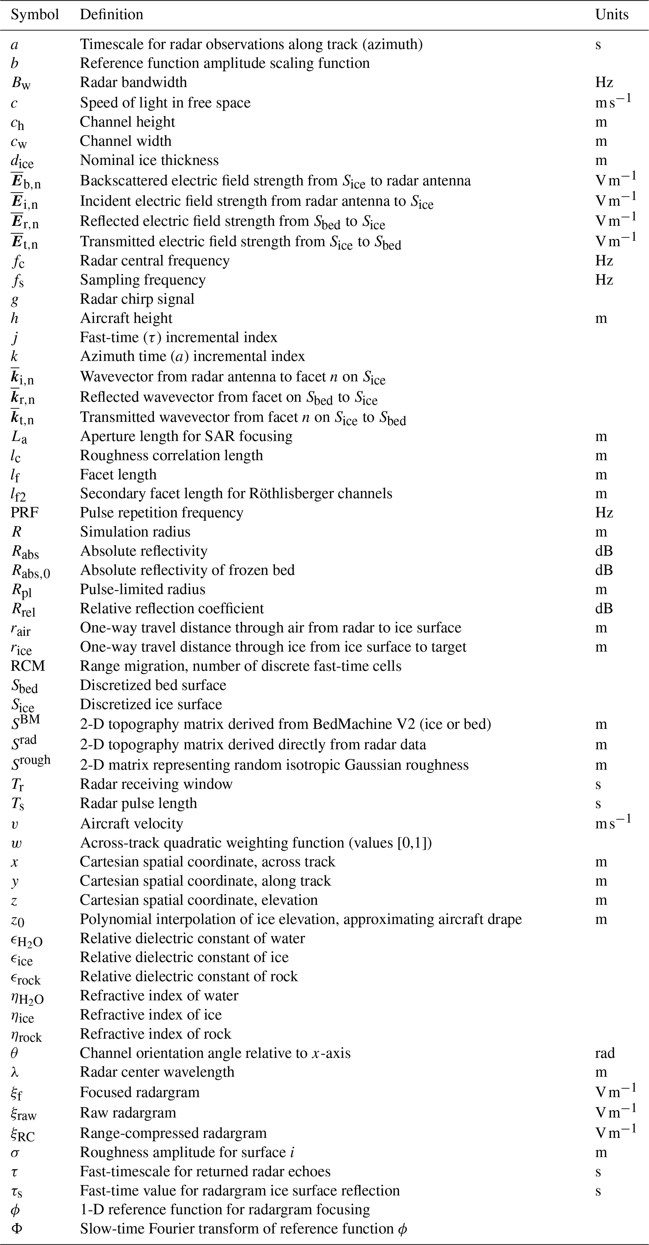
- Appendix B: List of variables used in this paper
- Data availability
- Author contributions
- Competing interests
- Disclaimer
- Acknowledgements
- Financial support
- Review statement
- References
- Abstract
- Introduction
- Simulation methodology
- Results – hypothetical simulation cases
- Application to Thwaites Glacier
- Discussion
- Conclusions
- Appendix A: Along-track focusing
- Appendix B: List of variables used in this paper
- Data availability
- Author contributions
- Competing interests
- Disclaimer
- Acknowledgements
- Financial support
- Review statement
- References