the Creative Commons Attribution 4.0 License.
the Creative Commons Attribution 4.0 License.
 | 27 Mar 2024
Sea-ice variations and trends during the Common Era in the Atlantic sector of the Arctic Ocean
Ana Lúcia Lindroth Dauner
Frederik Schenk
Katherine Elizabeth Power
Maija Heikkilä
Sea ice is crucial in regulating the heat balance between the ocean and atmosphere and quintessential for supporting the prevailing Arctic food web. Due to limited and often local data availability back in time, the sensitivity of sea-ice proxies to long-term climate changes is not well constrained, which renders any comparison with palaeoclimate model simulations difficult. Here we compiled a set of marine sea-ice proxy records with a relatively high temporal resolution of at least 100 years, covering the Common Era (past 2k years) in the Greenland–North Atlantic sector of the Arctic to explore the presence of coherent long-term trends and common low-frequency variability, and we compared those data with transient climate model simulations. We used cluster analysis and empirical orthogonal functions to extract leading modes of sea-ice variability, which efficiently filtered out local variations and improved comparison between proxy records and model simulations. We find that a compilation of multiple proxy-based sea-ice reconstructions accurately reflects general long-term changes in sea-ice history, consistent with simulations from two transient climate models. Although sea-ice proxies have varying mechanistic relationships to sea-ice cover, typically differing in habitat or seasonal representation, the long-term trend recorded by proxy-based reconstructions showed a good agreement with summer minimum sea-ice area from the model simulations. The short-term variability was not as coherent between proxy-based reconstructions and model simulations. The leading mode of simulated sea ice associated with the multidecadal to centennial timescale presented a relatively low explained variance and might be explained by changes in solar radiation and/or inflow of warm Atlantic waters to the Arctic Ocean. Short variations in proxy-based reconstructions, however, are mainly associated with local factors and the ecological nature of the proxies. Therefore, a regional or large-scale view of sea-ice trends necessitates multiple spatially spread sea-ice proxy-based reconstructions, avoiding confusion between long-term regional trends and short-term local variability. Local-scale sea-ice studies, in turn, benefit from reconstructions from well-understood individual research sites.
- Article
(4431 KB) - Full-text XML
-
Supplement
(3135 KB) - BibTeX
- EndNote


Sea ice is crucial in regulating the heat balance between the ocean and the atmosphere and plays a major role in the Arctic food web (Arrigo, 2014; IPCC, 2021). Despite the importance of sea ice for ecosystems and climate, reconstructing its history remains challenging (Heikkilä et al., 2022). While the development of palaeoceanographic sea-ice proxies has progressed in recent decades (de Vernal et al., 2013; Belt, 2019; Weckström et al., 2020), they often exhibit strong local and regional dependencies, limiting their use for large-scale extrapolation (Brennan and Hakim, 2022). In contrast, longer transient palaeoclimate simulations of large-scale sea-ice changes using numerical models have only recently become available (Zhong et al., 2018; Mauritsen et al., 2019). Therefore, the identification and distinction between average long-term trends and regional and internally forced variability has remained a challenge.
Sea ice affects global and regional climate systems through its role in modification of water and energy budgets (Macias-Fauria and Post, 2018; Kretschmer et al., 2020; IPCC, 2021). It acts as a physical barrier, reducing or close to preventing heat and moisture transfers between the ocean and the atmosphere, which has significant impacts on weather and climate (Bintanja, 2018; Sun et al., 2018). Also, sea ice reflects a large part of incoming solar radiation back to space due to its high surface albedo, moderating ocean warming at high latitudes (Bader et al., 2020). A reduction in high-latitude surface albedo causes a non-linear response known as Arctic amplification – a phenomenon in which northern high latitudes are warming 2 to 4 times faster than the global mean (Dai et al., 2019; Rantanen et al., 2022; Ryan et al., 2022). In addition to being a key climate parameter, sea-ice presence is fundamental to Arctic marine ecosystems. Sea ice provides a unique habitat for diverse biological communities formed by ice-dwelling (sympagic) and ice-dependent species (Eamer et al., 2013; Arrigo, 2014). While multiyear sea ice provides a year-round habitat that supports endemic Arctic species, areas seasonally covered by sea ice have the highest marine primary production by ice algal and phytoplankton blooms during the melt and open-water seasons (Hop and Gjøsæter, 2013; Lannuzel et al., 2020).
A major challenge for comprehending the consequences of present climate change on sea-ice and Arctic marine ecosystems is the lack of baseline data (Heikkilä et al., 2022). Although limited historical sea-ice observations (mainly based on ship logbooks) exist (Vinje, 2001; Divine and Dick, 2006; Schweiger et al., 2019), most human observations of sea ice are derived from satellites and date back only to the 1970s (Fox-Kemper et al., 2021). Palaeoclimate data derived from marine sediments can provide insights into Arctic environmental change over much longer timescales. However, most Arctic palaeoclimate data compilations so far have focused on past temperatures, and the majority of the compiled data originate from terrestrial environments. For example, McKay and Kaufman (2014) compiled 56 records in an Arctic proxy temperature database for the past 2000 years, but only 6 record ocean temperatures. More recently, a global temperature reconstruction for the Common Era (CE) compiled more than 200 proxy records, but none of the marine-related reconstructions were located in the Arctic Ocean (PAGES 2k Consortium, 2019).
To our knowledge, there are only two proxy-based data compilations of past sea-ice cover (Kinnard et al., 2011; Brennan and Hakim, 2022), neither of which focuses on marine sea-ice proxies. Kinnard et al. (2011) reconstructed sea-ice conditions over the past 1450 years using ice-core records, tree-ring chronologies and lake sediments. Brennan and Hakim (2022) assimilated temperature-sensitive proxy records from tree rings, ice cores, corals, lake sediments and bivalve records into a numerical model to study Arctic sea-ice conditions during the Common Era. However, a wealth of evidence of past sea-ice evolution during the Common Era have been made using sea-ice proxies preserved in marine sediments, typically microfossil assemblages (e.g. Sha et al., 2017; Tsoy et al., 2017; Allan et al., 2018) and source-specific algal lipids (e.g. Belt et al., 2010; Cabedo-Sanz et al., 2016; Detlef et al., 2021). Past sea-ice reconstructions based on microfossils rely on the presence and abundance of species associated with the presence of seasonal sea ice, typically diatoms or resting stages (cysts) of dinoflagellates (de Vernal et al., 2013; Weckström et al., 2020). Highly branched isoprenoid (HBI) lipids linked with sea-ice environments are increasingly common in sea-ice reconstructions, in particular IP25 (“ice proxy with 25 carbon atoms”). This lipid is produced by a few strictly sympagic diatoms and has a strong link to seasonal sea-ice presence and concentration (Belt, 2019). Although the use of sea-ice proxies is becoming more widespread, local and regional forcings (such as nutrient availability and freshwater and sediment contributions from land) might affect the organisms whose sedimentary remains are used in sea-ice reconstructions (Brown et al., 2020; Luostarinen et al., 2020, 2023; Marret et al., 2020). Therefore, individual sea-ice reconstructions likely incorporate noise from local sea-ice characteristics and forcings other than regional-scale sea-ice cover. There are studies integrating multiple sampling sites or sediment cores, often describing and visually comparing sea-ice evolution among the records (e.g. de Vernal et al., 2013; Maffezzoli et al., 2021). However, an integration of existing sea-ice reconstructions in a systematic way for the entire northern North Atlantic to underline main trends and/or variability has, so far, not been undertaken.
Combining proxy data synthesis with climate model outputs may allow us to distinguish local sea-ice changes from large-scale variability, complementing and strengthening the interpretation of past sea-ice evolution (Moffa-Sánchez et al., 2019; Brennan and Hakim, 2022). In contrast to proxies, numerical models offer improved spatial coverage and temporal resolution and can provide a coherent and physically consistent overview of the climate on varying timescales, although large model biases exist in Arctic regions, attributable to complex feedback frameworks and remaining deficiencies in the implementation of sea ice in general circulation models (Goosse et al., 2013, 2018). Though the majority of simulations contributing to the latest Coupled Model Intercomparison Project (CMIP6) included sea ice as a variable, detailed evaluations of sea ice in palaeoclimate simulations are still pending, as long transient simulations and more sea-ice proxies have become available only recently (Zhong et al., 2018; Mauritsen et al., 2019).
Here, we use high-resolution sea-ice reconstructions based on palaeoceanographic proxies together with numerical model outputs to identify possible common trends and/or regional differences in the evolution of sea-ice cover over the Common Era in the Atlantic sector of the Arctic Ocean. We also aim to probe whether sea-ice proxies (microfossils and IP25) are suited to capture large-scale sea-ice changes or if local forcings have a larger influence. Lastly, we discuss the external forcings that may be causing the sea-ice changes observed in our study.
2.1 Data
Palaeoceanographic datasets were obtained from the databases by NOAA (https://www.ncei.noaa.gov/access/paleo-search/, last access: 30 June 2021), PANGAEA (https://www.pangaea.de/, last access: 30 June 2021) and Neotoma (https://www.neotomadb.org/, last access: 30 June 2021) between January and June 2021. Additional published records that were not found in these databases were solicited from the original authors. Based on the availability of suitable records, we focused on sediment cores retrieved from high latitudes (> 55° N) and the Atlantic sector of the Arctic Ocean (90° W to 30° E) that covered at least 80 % of the CE and presented an average temporal resolution of < 100 years.
The search included data of concentrations of highly branched isoprenoid lipid IP25 derived from sympagic algae, the abundance of diatom indicator species (Fragilariopsis oceanica, Fragilariopsis reginae-jahniae and Fossulaphycus arcticus) and the abundance of dinoflagellate cyst indicator species (Islandinium minutum and I.? cezare).
The biogeochemical proxy IP25 was chosen due to its source-selectivity, as it is produced only by certain sympagic diatoms that are common across the Arctic Ocean (Belt, 2018). This lipid is produced in the ice during the sympagic spring bloom prior to ice melt, and it is, therefore, interpreted as a proxy measure of seasonal sea ice. Since IP25 is not produced in ice-free areas or under permanent/extensive sea-ice cover due to light limitation, changes in its concentration are interpreted in terms of fluctuations in seasonal sea-ice area (Belt, 2019).
Microfossils of sympagic diatoms are typically not found in sediments (Limoges et al., 2018; Luostarinen et al., 2023). Thus, the diatom indicator species for sea ice are those that bloom in abundance under the ice or at the ice edge during spring melt. These species can be found in small concentrations within the ice matrix, indicating blooms seed in the ice matrix, while their main occurrence is in the stratified waters in the marginal ice zone. Fossulaphycus arcticus, Fragilariopsis reginae-jahniae and Fragilariopsis oceanica present a significant relationship with high April sea-ice concentrations in the Atlantic Arctic (Weckström et al., 2020).
The dinoflagellate cyst indicator species Islandinium minutum and I.? cezare were also chosen due to their affinity with seasonally sea-ice-covered regions. They are found most abundantly in surface sediments in Arctic areas that experience seasonal sea ice and are mainly associated with cold waters from polar to subpolar regions (Head et al., 2001; de Vernal et al., 2020). Their ecological connection to sea-ice cover is, however, unresolved. Recently, for example, Luostarinen et al. (2023) observed that these species were virtually absent in sea ice, water column and sediment flux during spring melt although being common in surface sediments.
Concentration data were obtained in the form of mass of IP25 either related to sediment dry weight (µg g−1 dw or ng g−1 dw, with dw meaning dry weight) or normalized by total organic carbon (µg g−1 TOC or ng g−1 TOC). When both options were available, we prioritized IP25 concentrations normalized by TOC. Diatom and dinoflagellate cyst abundance data were retrieved as indicator species proportion (%) of the total species assemblage. We decided to focus only on measured proxy concentrations and abundances instead of quantitative estimates of reconstructed sea-ice concentrations and sea-ice duration. This is because quantitative reconstructions incorporate species assemblages, including taxa not related to sea ice and primarily controlled by other environmental factors. Furthermore, the mechanistic relationships of many of the proxies to the reconstructed environmental parameter are still not thoroughly understood (Heikkilä et al., 2022). Importantly, while each proxy record used here is based on measured quantities, the proxies represent a relative measure of seasonal sea-ice concentrations rather than geophysical quantities.
The chronologies were based on radiocarbon dating (accelerator mass spectrometry 14C), and the original age–depth models were used.
2.2 Numerical models
Two climate simulations covering the past 2000 years (2k hereafter) were used. These are the Max Planck Institute Earth System Model 1.2 Low Resolution (MPI-ESM1.2-LR; hereafter MPI-ESM; Mauritsen et al., 2019) which was used to perform past 2k transient simulations (Jungclaus et al., 2017; van Dijk et al., 2022), and the Community Earth System Model 1.1 (CESM1.1/CCSM4; hereafter CESM1) “past2k” transient simulation (Zhong et al., 2018). Both models contributed to the PMIP (Paleoclimate Modelling Intercomparison Project) as part of the Coupled Model Intercomparison Project Phase 6 (CMIP6) (Jungclaus et al., 2017).
The MPI-ESM consists of four model components: ocean dynamical model MPIOM1.6, ocean biogeochemistry model HAMOCC6, atmosphere model ECHAM6.3 and land model JSBACH3.2. These are coupled together via the OASIS3-MCT coupler. The configuration used is ∼ 150 km in the ocean and ∼ 200 km in the atmosphere, with 47 atmospheric vertical levels (Mauritsen et al., 2019). CESM1 is also a global fully coupled model consisting of four component models: atmospheric model (AGCM), ocean model (OGCM), land surface model (CLM) and sea-ice model (CICE) connected by a central coupler (Craig et al., 2012). It has a ∼ 1° resolution in the ocean and sea ice and ∼ 2° resolution in the atmosphere (Zhong et al., 2018).
Both simulations are transient, meaning they start from past climate boundary conditions, but the exact starting time varies. They then simulate the climate forward through the past2k. Forcing data for the past2k experiments is based on the PMIP4 protocol (Jungclaus et al., 2017). For CESM1, forcings are solar irradiance and volcanic aerosols (Toohey et al., 2016), land use and land cover (Klein Goldewijk et al., 2010), and greenhouse gas levels (MacFarling Meure et al., 2006). For both simulations, orbital forcing is from Berger (1978). For MPI-ESM, forcings include solar irradiance (Krivova et al., 2011), land use (Hurtt et al., 2011) and greenhouse gas levels (Brovkin et al., 2019). The only variable studied is sea-ice fraction, specifically “sea-ice area percentage” (Siconca) from MPI-ESM and “fraction of surface area covered by sea ice” (Icefrac) from CESM1. These represent the percentage of ice cover in each grid square, and both variables are on atmospheric grids. Extratropical (30–60° N) surface air temperature is used in addition for model comparison (Fig. 4).
2.3 Statistical analyses
Maps were made using QGIS (QGIS Development Team, 2022). All statistical analyses were performed in the R environment (R Core Team, 2022).
Prior to statistical analyses, all proxy datasets were standardized to allow for a direct comparison among data from disparate sources. Z scores were calculated by subtracting the data by the mean and dividing by the standard deviation of each record, considering only data dated to the Common Era. To allow for statistical comparisons, all datasets were reduced to a common resolution by binning to the same 100-year time slices (the top sample, centred at 1950 CE, integrating the time slice 1900–2000 CE, and so on) (Shuman et al., 2018).
A cluster analysis using SAX (Symbolic Aggregate approXimation) representation (Lin et al., 2007) in the dissimilarity measure calculation was used to categorize the marine proxy records into groups according to their evolution through time. SAX representation is a “structure-based” dissimilarity measure that focuses on comparing underlying dependence structures and is thus suitable for time-series analyses. The symbolization approach involves transformation of time series into sequences of discretized symbols, allowing for dimensionality reduction but keeping the distance measures defined on the original time series (Lin et al., 2007). Thus, this approach can be used to group different proxy records according to their temporal evolution, regardless of their units. For example, sea-ice reconstructions with similar patterns, such as a continuous increase, would be grouped together, separated from sea-ice reconstructions with a continuous decrease pattern. The cluster analysis was repeated using the globally (over all used records) detrended records to remove the overall dominant influence of the global trend. For this, we calculate the average of each time step of the z-score records (the global trend) and subtracted this average from each of the z-score records. Finally, the data pertaining to each group were averaged, in order to create a unique record for each group. The “TSclust” package (Montero and Vilar, 2014) was used to run the cluster analyses and the “zoo” package (Zeileis et al., 2022) was used to deal with the missing values.
For the exploration of the climate models, we used annual sea-ice minimum and maximum of monthly mean data. Sea-ice areas (km2) were calculated by multiplying the sea-ice fraction in each grid (%) by its grid area (km2) and summing the area of all grids, which gives the annual area. For better visualization, the data were smoothed with a 100-year running mean. To mimic the behaviour of our proxy records, we repeated the analysis using 100-year mean chunks, e.g. for the empirical orthogonal function (EOF) analysis. The “mean chunks” are meant to highlight that non-overlapping mean segments are used, mimicking the samples of proxy records. Pearson correlation analyses were calculated between sea-ice areas from the whole Arctic Ocean and from the region around Greenland using the package “Hmisc” (Harrell, 2022).
All model data were filtered using a low-pass red noise Butterworth filter to remove sub-decadal (< 10 years) oscillations using the “signal” package (Ligges et al., 2022). A wavelet analysis (Morlet wavelet) was performed using the sea-ice areas (annual resolution) to identify significant oscillations that could show coherence between different datasets or represent unforced variations, using the “WaveletComp” package (Roesch and Schmidbauer, 2018). During the analysis, the data were internally detrended using a degree of time-series loess smoothing of 0.75; a total of 100 simulations were performed, and the used method to generate surrogate time series was a first-order autoregressive model (AR-1). Wavelet analyses were also performed using the proxy data, using the same parameters. As proxy data do not have the resolution to analyse sub-decadal variability, high-frequency variability was filtered out in model runs with a low-pass filter to be consistent with proxy data.
Additionally for the model data, we applied an empirical orthogonal function (EOF) analysis for the unfiltered sea-ice fraction data to identify the main modes of variability and their spatial representation. Prior to EOF analysis, we applied a log transformation of the fractional data using log10 after adding an arbitrary offset of 0.5 to avoid zeroes, which would be a problem for the log transformation. The log transformation helps to avoid the sharp cut-off at 0 and 1 that does not exist for the other variables that we compare with (proxies and simulated temperature, etc.). It also helps to normalize the data distribution and reduce skewness and heteroscedasticity to make data comparable with non-fractional data. In order to test the applicability of the 100-year time slices used for the proxy data, we calculated the EOFs using annual data, the 100-year running mean and the 100-year mean chunks. They all presented similar results, considering both EOF1/2 and PC1/2, and in this study we are presenting EOFs and PCs based on the smoothed 100-year running mean data and also the PCs based on the 100-year time slices. EOFs were calculated with CDO version 1.9.10 (Schulzweida, 2021).
Other packages used during the analyses were “dplyr” (Wickham et al., 2022) to clean and organize the data and “ncdf4” (Pierce, 2015) to import the files produced by CDO into R.
3.1 Proxy-based sea-ice reconstructions
Based on our spatial, temporal and resolution criteria, we retrieved 14 sea-ice reconstructions from 13 different sites (Fig. 1, Table 1). Twelve of them were based on IP25 concentrations and two were based on dinocyst assemblages. Unfortunately, there were no sea-ice records based on diatoms fitting our criteria of sufficient time coverage and resolution and geographical boundaries.
When dealing with individual sedimentary records, increases in IP25 concentrations and in dinoflagellate indicator species are associated with regional increases in the presence of seasonal sea-ice cover (de Vernal and Marret, 2007; Belt and Müller, 2013). Similarly, in this case, we assumed that increases observed in the temporal reconstruction for each cluster group refer to increases in sea-ice cover. For the temporal reconstruction of the cluster groups to present an increase in the z scores, this increase must have been observed in the individual records, scattered in different regions of the studied area. Because most of the cores are located in regions that have not been covered, during the Common Era, by multiyear sea ice, an increase in seasonal sea ice in different areas can be interpreted as an overall increase in sea-ice cover. Also because of the lack of perennial ice cover on most regions, the unimodal response of IP25 to sea ice was discussed in detail only in the regions where it might be relevant.
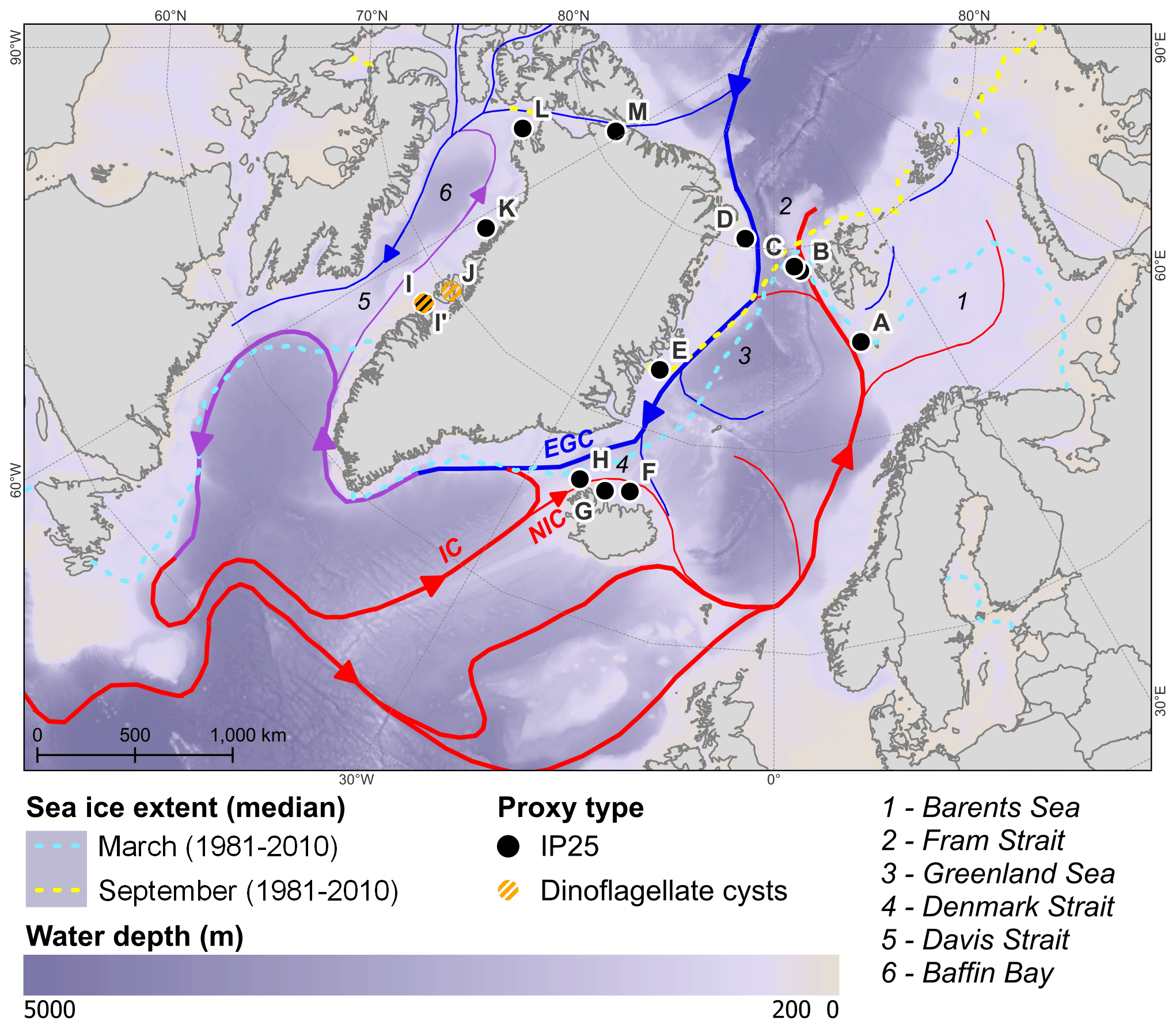
Figure 1Map showing the locations of IP25 and dinoflagellate cyst records for sea-ice reconstructions. The major surface currents are shown (blue: cold waters; purple: mixed water; red: warm waters), but only the currents discussed in the text are identified. EGC: East Greenland Current; IC: Irminger Current; NIC: North Irminger Current. The bold black line indicates the area used for the numerical model calculations. The bathymetry was obtained from Amante and Eakins (2009), the currents were plotted based on Talley et al. (2011a, b), and the median sea-ice extent was obtained from NOAA-NSIDC.
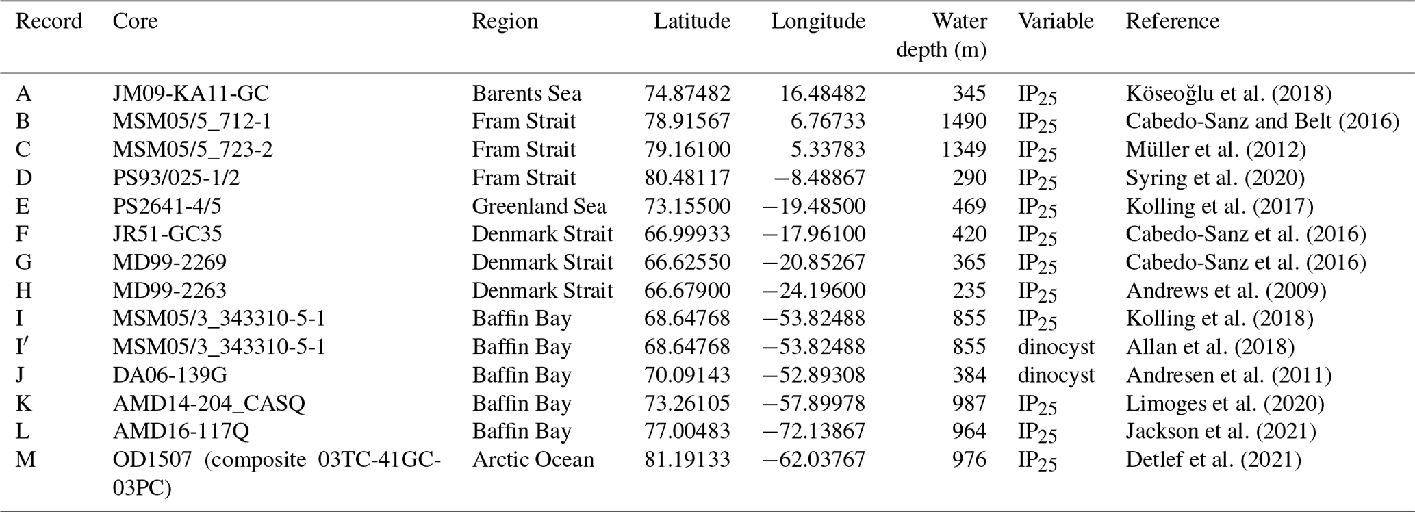
Table 1Marine record data including latitude, longitude, water depth and analysed variables.
All sea-ice proxy records were initially clustered in the same group (Fig. 2a), indicating that the 14 sea-ice reconstructions shared a similar overall pattern. This evidences that all records were under the influence of the same dominant forcing, producing a common trend (Fig. 2b). This overall increase in sea-ice cover agrees with the reconstructed neoglacial cooling in the Arctic (McKay and Kaufman, 2014) and globally (PAGES 2k Consortium, 2019), especially between 1200 and 1600 CE (Fig. 2b, Table S1 in the Supplement). The cooling trend and sea-ice expansion has been largely explained by the decrease in the Northern Hemisphere insolation due to orbital changes (Wanner et al., 2011) (Fig. 2c). In addition, the cumulative effect of large volcanic eruptions may have contributed to this long-term cooling (Büntgen et al., 2020), culminating in the Little Ice Age (LIA; 1600–1850 CE in the Arctic; Wang et al., 2022) (Fig. 2d). A recovery from the LIA starting around 1850 CE marks a remarkable change in the sign of trends (Fig. 2b). More recently, Arctic warming and sea-ice decrease have been accelerated by anthropogenic greenhouse gas emissions and land use changes (IPCC, 2021).
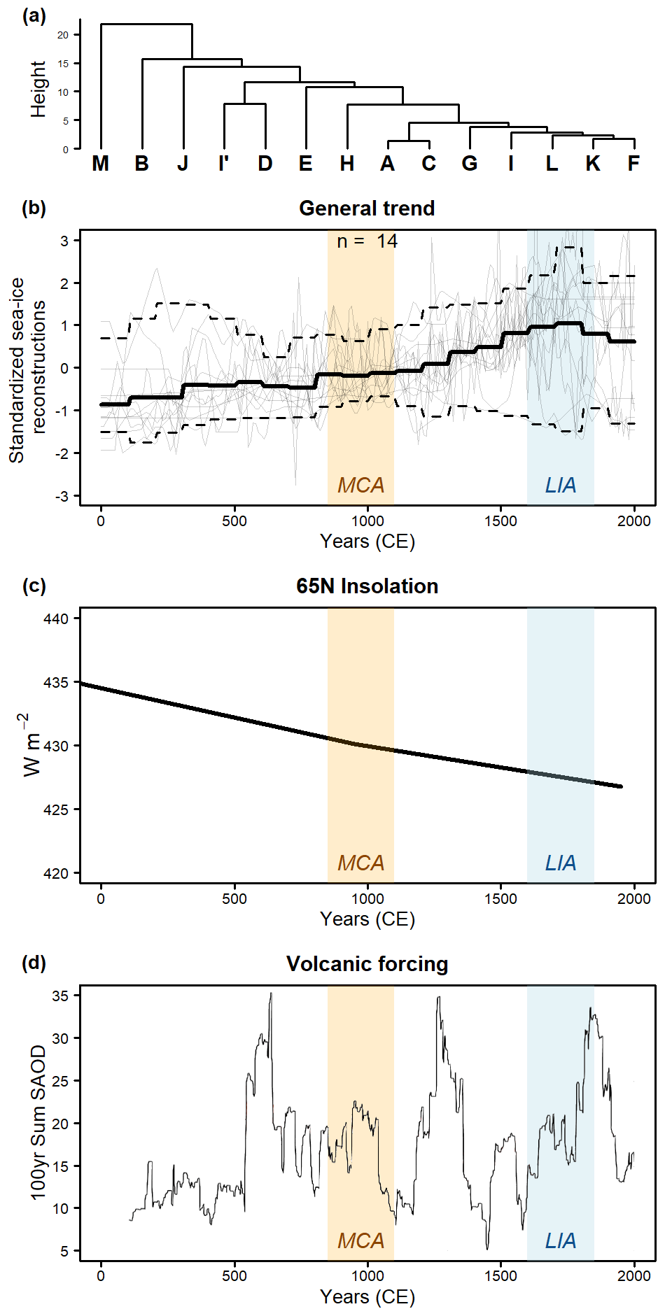
Figure 2(a) Dendrogram from cluster analysis and (b) average composite of the standardized sea-ice reconstructions used in this study. The solid line represents the mean values of all records, the thin grey lines show the individual standardized sea-ice reconstructions, and the dashed lines represent the amplitude of the standardized values after binning to 100-year time slices. All records witness a common sea-ice expansion trend until around 1850 CE, suggesting that they were under the influence of the same dominant forcing. (c) Insolation at 65° N from Berger and Loutre (1991). (d) Total stratospheric aerosol optical depth – SAOD from Büntgen et al. (2020). Larger SAOD values are indicative of larger volcanic dust inputs to the atmosphere. The translucent orange and blue areas indicate the Medieval Climate Anomaly (MCA) and Little Ice Age (LIA) for the Arctic region (Wang et al., 2022).
In addition to the common trend, the individual proxy records presented a large variability, especially in the first and last five centuries of the Common Era (Fig. 2b). The variability observed in the sea-ice reconstructions is probably caused by other environmental changes than the large-scale expansion/retraction of sea-ice cover. On both sides of Greenland, for example, the intrusion of warm Atlantic water has been suggested as the cause of the observed short-term variability in proxy-based sea-ice records (Kolling et al., 2017; Jackson et al., 2021). Changes in the position of the atmospheric polar front (Allan et al., 2018) and interactions with ice produced within fjords (Kolling et al., 2017) have also been suggested as explanations of this variability.
Although all records witness a common forced trend, a large spread in records in the early and late part of the Common Era indicate the presence of other local variability. To identify such second- and higher-order variations, we removed the common non-linear trend (the average composite observed in Fig. 2b) from all records and repeated the cluster analysis with the now regionally detrended data. When the general trend in the proxy records was removed, three distinct groups emerge from the cluster analysis (Fig. 3a). Importantly, the three groups (types of sea-ice evolution) do not form geographical entities. Instead, the sites within each group have sites located on both the western and eastern side of Greenland.
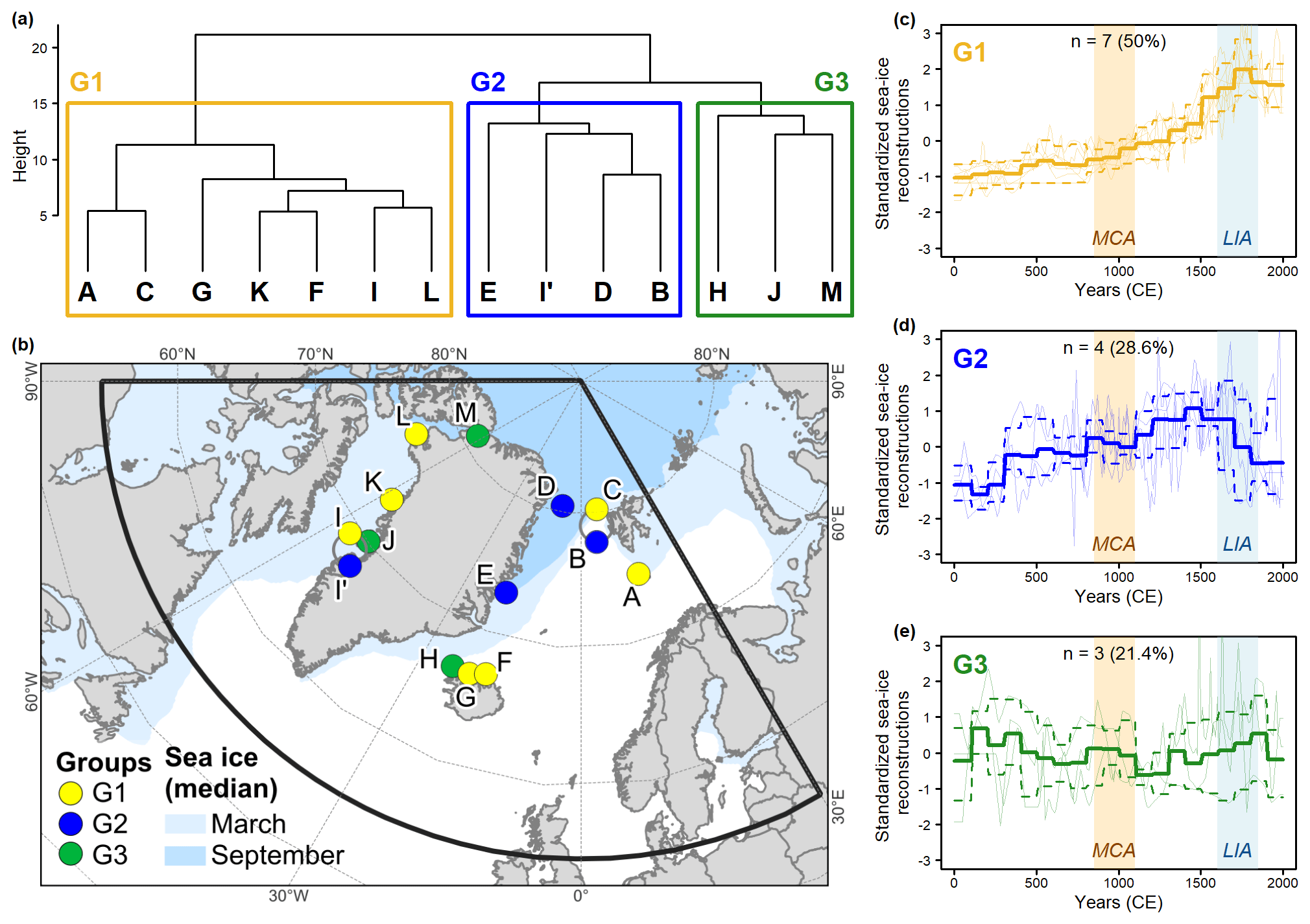
Figure 3Dendrogram (a) and average composite (c, d, e) of the standardized sea-ice reconstructions used in this study after removing the main trend (global average). The solid thick lines represent the mean values of all records, the thin lines show the individual standardized sea-ice reconstructions, and the dashed lines represent the amplitude of the standardized values after binning to 100-year time slices. The spatial distribution of records in each cluster is presented in panel (b). The solid thick black line in panel (b) represents the spatial domain used in the climate simulations. The translucent orange and blue areas in plots (c), (d) and (e) indicate the Medieval Climate Anomaly (MCA) and Little Ice Age (LIA) for the Arctic region (Wang et al., 2022). Most records suggest a sea-ice expansion (G1 and G2), followed by a retraction after the 18th (G1) and 16th (G2) centuries. G3 groups local records from scattered locations that do not follow the previously described sea-ice expansion trend in G1 or G2.
The first group (G1; Fig. 3c and Table S1) presented practically the same pattern as in the general trend (Fig. 2), with maximum sea-ice cover around 1750 CE, corresponding with the LIA in the Arctic (1600–1850 CE; Wang et al., 2022). Group 1 includes three records from Baffin Bay, two records retrieved off Svalbard and two records from northern Iceland. While Baffin Bay is currently under the influence of seasonal sea-ice cover, the other four records were collected in regions south of the current winter sea-ice edge (Fig. 1). The sea-ice expansion demonstrated by G1 until 1750, even after removing the general trend (Fig. 2), highlights the importance of large-scale processes at these sites, such as transient changes in orbital forcing in combination with volcanism causing atmospheric cooling and consequent sea-ice expansion. Massé et al. (2008) reported the highest IP25 concentrations over the past millennium during the 17th and 19th centuries in the Iceland Sea, in agreement with maximum sea-ice area at that time. Interestingly, G1 demonstrates a higher rate of sea-ice increase from 1600 CE until the end of the LIA, which is not apparent in the general trend (Fig. 2). While the sea-ice proxy compilation suggests a rather gradual cooling trend, episodic snowline lowering and ice cap expansion in Arctic Canada highlight that part of the cooling trend is enhanced during periods of explosive volcanism (Miller et al., 2023) that is not clearly visible in nearby sea ice.
Considering individual records and local variability, Cabedo-Sanz et al. (2016) and Miles et al. (2020) suggest that this apparent accelerating expansion of sea ice south of the Fram Strait might be caused by more sea-ice export by stronger southward currents (mainly the East Greenland Current) carrying polar waters and pack ice. Thus, in addition to the sea-ice growth caused by the neoglacial cooling, ice was also transported to more southern latitudes by stronger currents. Following the maximum sea-ice cover during the LIA, a slight decreasing trend in sea ice is demonstrated by G1. However, out of the seven records in this group, only three (A, G and L) cover the modern industrial period (after 1850 CE) (Fig. S1 in the Supplement). While record G shows a decrease in the sea ice (Cabedo-Sanz et al., 2016), the other two records point to highly fluctuating sea-ice conditions (Köseoğlu et al., 2018; Jackson et al., 2021). Thus, the plateauing trend in the last century might be an artefact of the analysis, since four of the records did not have an adequate time coverage for the modern period (Fig. S1).
Group 2 (G2; Fig. 3a) is a cluster of four proxy records collected in the Fram Strait (B, D), off eastern Greenland (E) and near Davis Strait, off western Greenland (I′; Fig. 3b). This group shares the general trend of sea-ice expansion in the beginning of the Common Era with G1 (Fig. 2), but the maximum values are reached a few centuries earlier, between 1250 and 1650 CE. In addition, the decreasing trend following the sea-ice maximum is more distinct (Fig. 3d and Table S1). A similar pattern was observed in polar and subpolar species of foraminifera from the Fram Strait (core MSM05/5_712-1; Spielhagen et al., 2011). The relatively similar long-term trend between G1 and G2 until ∼ 1500 CE suggests a common response to a large-scale climate forcing where G2 includes temporal deviations from the overall similar trend. For the past 500 years, G2 diverges from the continued long-term trend in G1 showing an earlier decrease in sea-ice. Differing internal system responses and methodological constraints of IP25 proxy may have an influence on this deviation. The early sea-ice maximum in G2 was followed by a sea-ice decrease, especially in the two records from Fram Strait (B and D). This decrease is probably an artefact caused by the two end-member scenarios for absent IP25 in downcore records (Belt, 2018). While IP25 (produced by sympagic diatoms) is absent in ice-free oceans, thick, perennial sea ice also reduces sympagic diatom and thus IP25 production (Belt, 2018). Considering the record in their study, Cabedo-Sanz and Belt (2016) suggested that a switch from long seasonal sea-ice cover to a perennial sea-ice scenario could explain the early decrease in IP25 observed in Fram Strait. Another explanation by Kolling et al. (2017) and Syring et al. (2020) also suggests colder climate but coupled to more open-water conditions due to polynya (ice-free area) formation on the East Greenland shelf. It was probably caused by glacier expansion and katabatic winds pushing sea ice off the coast.
Considering the whole studied area in our study, the explanation of a cold climate but with ice-free areas also fits with the findings from the foraminifera data of Spielhagen et al. (2011), where the high fluxes of polar and subpolar species during the early LIA were associated with sea-ice margins. The apparent sea-ice retreat observed at I′ in Davis Strait, the only G2 site in the western side of Greenland, might be explained by the establishment of polynya conditions and an increase in sea-ice production along Greenland's western side. Polynyas are areas of open water and thin ice in regions otherwise covered by sea ice and are common around Greenland (Smith and Barber, 2007). The decrease in Islandinium minutum and I.? cezare is concomitant with an increase in the abundances of phototrophic taxa (especially Pentapharsodinium dalei), potentially indicating a shift towards longer open-water seasons (Allan et al., 2018).
Interestingly, some records from sediment cores retrieved from areas very close to each other were not necessarily assigned to the same cluster group (Fig. 3b). For example, a sea-ice decrease over the last 2 centuries was not observed in record I, a sea-ice reconstruction from the same sediment core as dinocyst record I′ (MSM05/3_343310), but based on IP25 (Kolling et al., 2018). The differing cluster allocation of the dinocyst record (I′, G2) and the IP25 record (I, G3) is caused by the difference in their temporal trends and temporal coverages. Although having a good temporal resolution of 14 years, record I (IP25) only covers the period until 1809, whilst record I′ (dinocysts) extends to 2006 (Figs. S1 and S2). Therefore, record I did not have an appropriate temporal coverage to register the potentially same decrease as observed in record I′.
The lack of temporal coverage is also the probable reason behind the assignments of records B and C in different groups, even though both sediment cores were retrieved from the eastern Fram Strait off Svalbard (Fig. 3). While record B was assigned to Group 2 due to the decrease in IP25 after the 15th century (Fig. S2), record C was placed in Group 1. However, record C only covers the time until 1770 CE (Fig. S1). Therefore, it does not have enough temporal coverage to register a potential IP25 decrease.
Lastly, Group 3 (G3; Fig. 3a) is formed by three records and presents no clear long-term trend. This group contains records that did not fit into the two previous groups rather than records with a similar sea-ice evolution (Fig. 3e and Table S1). Sediment core OD1507 (composite 03TC-41GC-03PC) (record M in Fig. 3b) is located inside a fjord and presents a long-term decrease in IP25 concentrations (Detlef et al., 2021). The authors of the original study argue that production of IP25 decreases with the establishment of near-perennial sea-ice cover during the Common Era. Therefore, we consider that the decrease in IP25 is probably caused by the two end-member scenarios for absent IP25, since perennial sea ice reduces sympagic blooms and IP25 production (Belt, 2018). Sediment core DA06-139G (record J in Figs. 3b, S3) was also collected inside a strait and was thus under the influence of land-fast sea ice and marine-terminating glaciers (Andresen et al., 2011). The lack of temporal trend might be related to the influence of freshwater coming from the continental ice sheets where atmospheric warming may increase melting and adversely cool the surface waters locally as can be observed in glacier-fed lakes during heatwaves (Kirchner et al., 2021). Limoges et al. (2018) advise about the use of IP25 in coastal areas, as lower salinities may influence the structural nature of sea ice and its propensity to sustain algal growth. Therefore, freshwater influence might cause a decline in IP25-producing diatom species.
The sediment core MD99-2263 (record H in Fig. 3b), on the other hand, is located off the Iceland shelf in an open-water environment and close to cores JR51-GC35 (F) and MD99-2269 (G). Putting the record in context along with these nearby records in our compilation, the main difference between records F and G (both assigned to Group 1) and record H (assigned to Group 3) occurred between 1450 and 1650 CE (Figs. S1 and S3). During this period in record H, high sediment accumulation rates coincided with relatively high concentrations of IP25 (Andrews et al., 2009). The authors suggest that in this location the sea-ice proxy IP25 was associated with increasing drift ice related to changes in the wind pattern during the European LIA. Stronger N and NW winds led to more sea ice being exported from the Arctic Ocean towards the NW or N Iceland shelf. However, this increment was not as noticeable as observed in records F and G. One possible explanation for this difference is the spatially diverse impact of stronger currents carrying warm waters in this region. Sediment core MD99-2263 (record H) was collected in the Denmark Strait, in a region directly under the influence of the North Irminger Current that carries warm Atlantic waters towards the Nordic Seas (Talley et al., 2011a). Sediment cores JR51-GC35 (F) and MD99-2269 (G), however, are located in a more protected region off northern Iceland. Between 1450 and 1650 CE, Europe was already under the influence of LIA unlike Greenland and North America (Wang et al., 2022). The difference in the temperatures caused a strengthening of the subpolar gyre, resulting in a stronger presence of warm and saline Atlantic water carried by the Irminger Current in the Denmark Strait region (Miettinen et al., 2012), where sediment core MD99-2263 (record H in Fig. 3) was retrieved. Thus, it is possible that during this period the presence of warm waters intensified the melting process of drift ice, promoting the transfer of sea-ice proxies from the ocean surface to the sediments. Around 1600, the onset of LIA in Arctic and North America (Wang et al., 2022) probably caused a weakening of the Atlantic currents towards the Nordic seas.
3.2 Model-based sea-ice reconstructions
Annual mean air temperature trends (Fig. 4) produced by both models in our study present a similar declining pattern as proxy-based Arctic temperatures obtained in a reconstruction by McKay and Kaufman (2014). The McKay and Kaufman (2014) reconstruction obtained a cooling of −0.49 °C kyr−1 for the Arctic region (latitude > 60° N) for the pre-industrial part of the Common Era (Fig. S4). A comparable but less pronounced cooling is simulated by the CESM1 and MPI-ESM models, with cooling rates of −0.28 and −0.21 °C kyr−1, respectively (Fig. S4). This implies that the reconstructed cooling trend is roughly twice as strong as in both simulations. After 1850, air temperatures present a shift towards a warming trend. In the McKay and Kaufman (2014) proxy reconstruction, the warming is 0.97 °C per 100 years, while the CESM1 and MPI-ESM models yield warming rates of 1.34 and 0.84 °C per 100 years, respectively (Fig. S4).
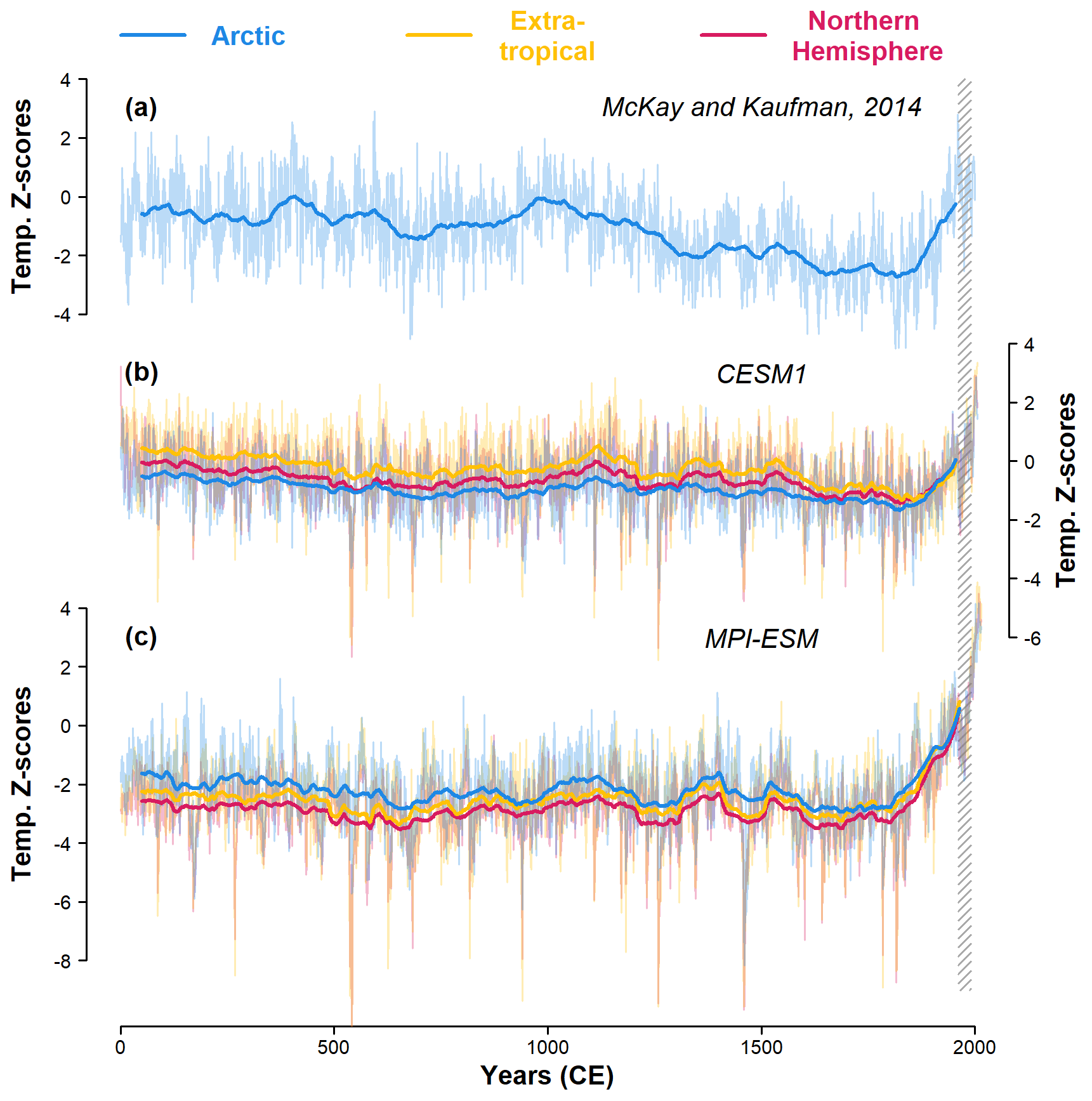
Figure 4Air temperature z scores (relative to the period between 1961–1990) based on (a) Arctic proxy data (McKay and Kaufman, 2014), (b) CESM1 simulation data and (c) MPI-ESM simulation data. Bold lines refer to 100-year running means. The area with hatching indicates the period between 1961–1990. Northern Hemisphere refers to latitudes between 0–90° N, the Arctic region refers to latitudes between 60–90° N, and the extratropical region refers to latitudes between 30–60° N. Temperature simulations from both models and for all three regions display a very similar long-term evolution, showing cooling temperatures for most of the Common Era, followed by a warming trend after 1850. This is consistent with the leading cluster G1 for the sea-ice proxies in Fig. 3c.
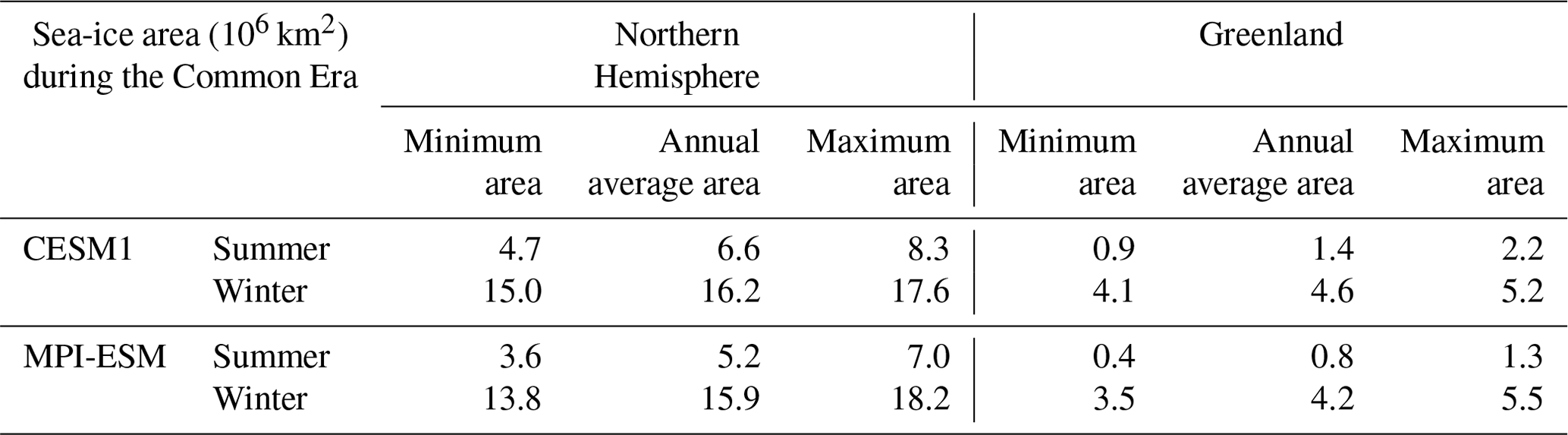
Considering the whole Arctic region and sea-ice area from both models for the period 0–2000 CE, CESM1 shows 27.4 % more summer sea ice than MPI-ESM (average areas: 6.6×10⁶ km2 vs. 5.2×10⁶ km2, respectively). During winter, the difference is very small and decreases to 1.7 %, with CESM1 presenting 16.1×10⁶ km2 of average sea-ice area and MPI-ESM presenting 15.9×10⁶ km2 (Table 2). There is less consistency in the region around Greenland with a strong difference during summer, with CESM1 showing 73.4 % more summer sea ice than MPI-ESM (average areas: 1.4×10⁶ km2 vs. 0.8×10⁶ km2, respectively) (Table 2). However, disregarding the magnitude and spatial bias of the sea-ice area, temporal changes in summer sea-ice area simulated around Greenland follow the changes as simulated for the whole Arctic Ocean (Fig. 5). Considering the 100-year running mean, the correlation of annual sea-ice area between the total Arctic Ocean and the region around Greenland is 0.92 for CESM1 and 0.93 for MPI-ESM during summer, and correlations are 0.57 for CESM1 and 0.94 for MPI-ESM during winter.
Table 2Comparison between simulated sea-ice areas (in ×106 km2) between the two models (CESM1 and MPI-ESM) for the Northern Hemisphere and for around Greenland (see mask in Fig. 1) for annual, summer and winter areas, over the Common Era (1–2000 CE).
When compared to the satellite data (Doerr et al., 2021), both models show slightly smaller summer sea-ice areas for the period between 1979 and 2000 (Table S2). While the numerical model simulated minimum summer sea-ice areas around 4.8×10⁶ km2 (CESM1) and 3.6×10⁶ km2 (MPI-ESM), sea-ice area calculations based on satellite data were around 5.4×10⁶ km2. The winter sea-ice areas, however, presented a good agreement between the results of the numerical model simulations and the satellite data. The numerical model simulated maximum winter sea-ice areas around 16.2×10⁶ km2 (CESM1) and 15.1×10⁶ km2 (MPI-ESM), and sea-ice area calculations based on satellite data were around 15.4×10⁶ km2.
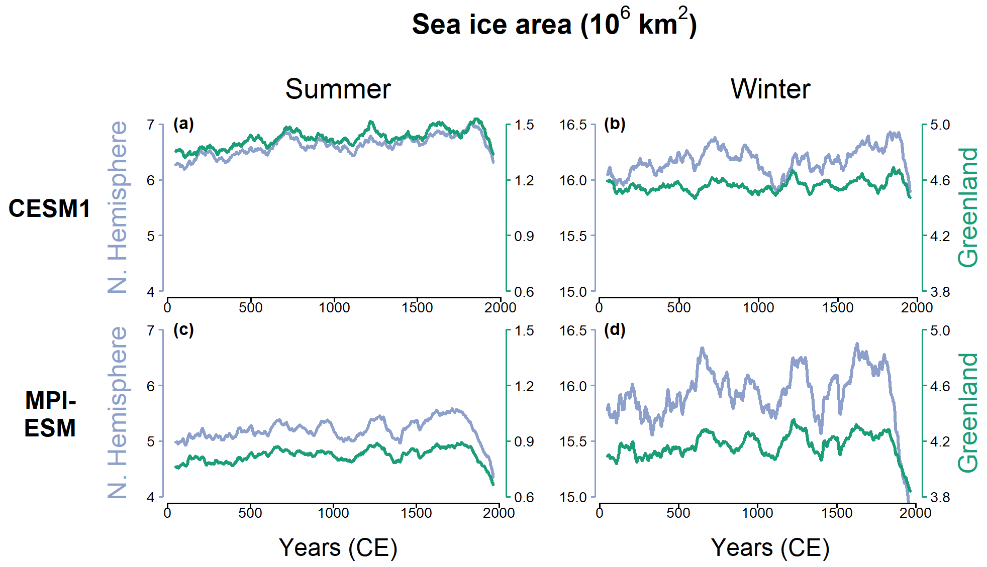
Figure 5Sea-ice area (in ×106 km2; 100-year running mean) in both models, around Greenland (green) and in the whole Northern Hemisphere (blue), for boreal summer and winter seasons, over the Common Era. The very high agreement indicates that sea-ice proxy-compilations around Greenland are representative for the total northern hemispheric sea-ice area on longer timescales. Disregarding magnitude bias, temporal changes in the sea-ice area simulated around Greenland follow the changes as simulated for the whole Arctic Ocean, especially during summer.
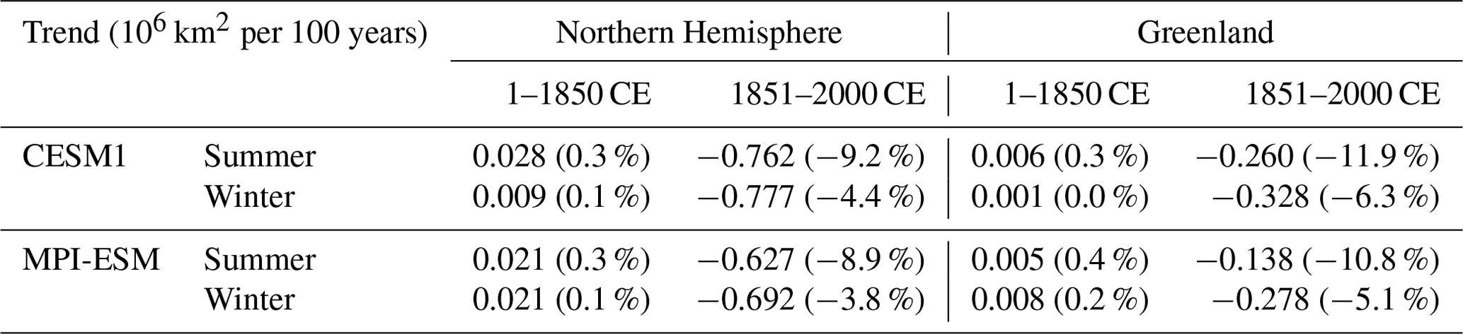
A general positive trend of increasing sea ice is simulated until 1850 for both seasons, followed by a sharp decrease in the sea-ice area due to global warming (Table 3). During the pre-industrial period of the Common Era, sea-ice areas simulated for the whole Northern Hemisphere suggest expansion rates around 0.02×10⁶ km2 per 100 years, and around 0.005×10⁶ km2 per 100 years when simulated for the region around Greenland. Nevertheless, the expansion rates are so small that when the maximum areas were compared over the centuries before 1850, the maximum sea-ice cover expanded less than 1 % per 100 years during the Common Era (Fig. S5). After 1850, however, the trend shifted, and both models registered decreases in sea-ice area. In the whole Northern Hemisphere, the simulated sea-ice area shrunk around 0.7×10⁶ km2 per 100 years (Table 3), corresponding to a loss of ∼ 9 % of area per 100 years during summer and ∼ 4 % of area per 100 years during winter, considering the maximum sea-ice area during the Common Era. Around Greenland, simulations suggest sea-ice shrinkage of around 0.2×10⁶ km2 per 100 years after 1850 (Table 3). When compared to the maximum sea-ice area simulated for the Common Era, it represents a decrease of ∼ 11 % area per 100 years in summer and ∼ 6 % of loss area per 100 years in winter (Fig. S5).
Table 3Comparison between trends of simulated sea-ice area (in ×106 km2 per 100 years) between the two models (CESM1 and MPI-ESM), in Northern Hemisphere and around Greenland (see mask in Fig. 1) and for boreal summer and winter seasons, over the Common Era (1–2000 CE). The percent (%) values consider the maximum sea-ice area simulated for the CE as reference.
To identify the main leading modes of sea-ice variability and their spatial loading patterns, we performed an EOF analysis for simulated sea-ice data after log transforming the fractional data. Overall, the EOF analysis using both the 100-year running mean and the 100-year mean chunk data yield very similar spatial and temporal patterns in the first mode of variability (EOF1 and PC1; Figs. S6 and S7). This similarity shows that the approach of creating 100-year mean chunks for the proxy data will retrieve the main temporal behaviour and likely does not create artificial patterns in the EOF analysis. As the sea-ice proxies are mainly related to the period of sea-ice melt, we will focus the discussion on summer sea ice, i.e. minimum annual area. Figure 6 shows the first and second mode of variability of summer sea ice. While the principal component plots (PC1 and PC2) present the results from both 100-year running mean and 100-year mean chunk data, the EOF1 and EOF2 plots only present the 100-year running mean results.
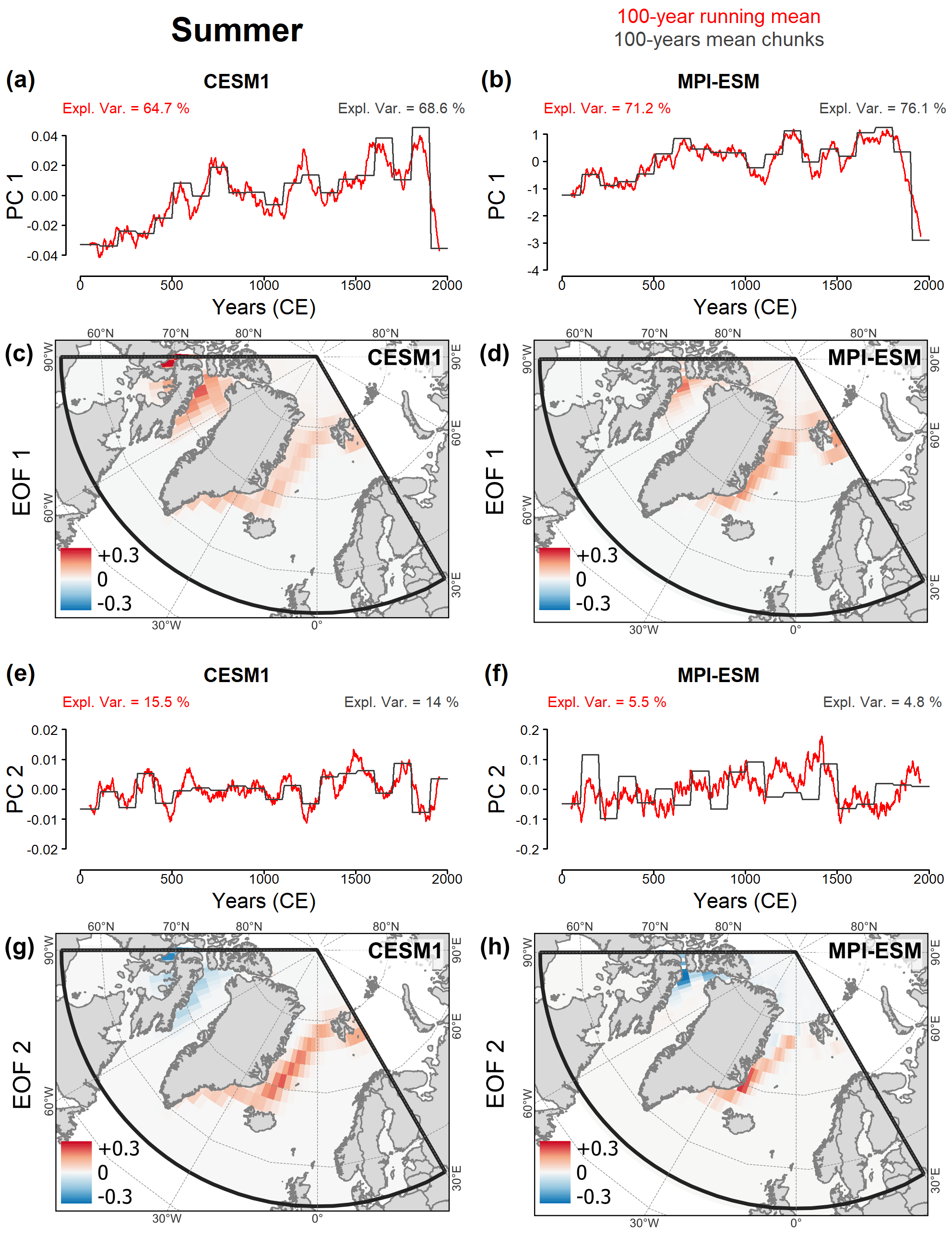
Figure 6Results of empirical orthogonal function (EOF) analysis of the log-transformed sea-ice fraction based on CESM1 (a, c, e, g) and MPI-ESM (b, d, f, h) data. Normalized principal components plots considering the 100-year running mean data (in red) and 100-year mean chunks, mimicking proxy data resolution (in dark grey); PC1: (a) and (b); PC2: (e) and (f). First and second EOF mode loadings plots consider the 100-year running mean data; EOF1: (c) and (d); EOF2: (g) and (h). In both models' simulations, the first mode captures most of the variability, with a sea-ice expansion trend during most of the Common Era followed by a sharp retraction in the last 2 centuries being simulated for the Labrador and Nordic seas. The second mode has a less clear temporal trend but displays an opposite pattern between the Labrador and the Nordic seas.
PC1 from both models (CESM1 and MPI-ESM) shows the expected long-term trend of increasing summer sea ice until around 1850 as in Fig. 5a and c, followed by a sharp decrease (Fig. 6a and b). The first leading mode explains more than 65 % of the variability in the CESM1 model and more than 70 % of variability in the MPI-ESM model. Spatially, most of the variance on multidecadal to centennial scales is concentrated in the Canadian channels and the Greenland Sea in both models (Fig. 6c and d). PC2, on the other hand, displays a temporal pattern governed by internal variability and explains only around 15 % and 5 % of the variability in CESM1 and MPI-ESM models, respectively (Fig. 6e and f). Although the temporal trends (PC2) were not quite similar between both models, the spatial structure of EOF2 presented the same opposite pattern between Baffin Bay and Greenland Sea in both models (Fig. 6g and h). This internal or residual variability might be related to changes in the sea-ice export through the Fram Strait. Given the low explained variance in the simulations, we would not expect a large explanatory value in the noisier sea-ice proxy data. Thus, the first leading mode appears to contain most of the interpretable variance on larger than centennial scales over the last 2 millennia for the chosen area.
In addition to the increasing summer sea-ice trend prior to 1850, PC1 in both models contains some quasi-periodic variability. This was also present in PC2. A wavelet analysis of the annual summer sea-ice area identified the main periodicities (Fig. 7). For CESM1, the multidecadal quasi-periodic variability is centred around 21, 33 and 74 years, and for MPI-ESM the variability is around 27, 41 and 74 years.
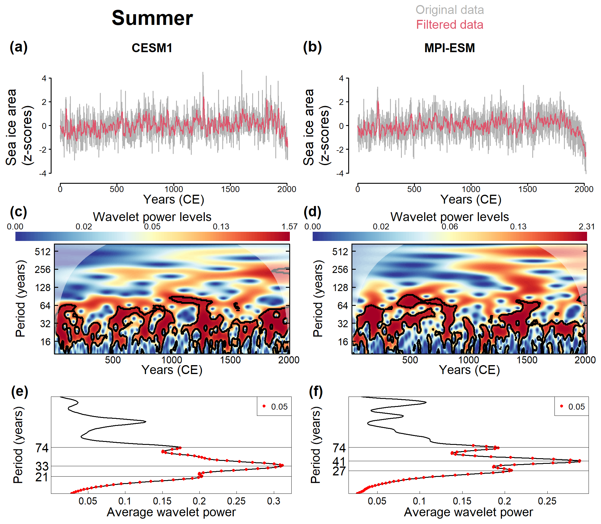
Figure 7Wavelet analysis from both numerical models (CESM1 and MPI-ESM), considering summer sea-ice area. (a, b) Normalized time series of sea-ice area considering the original data (in grey) and the filtered data (in red). (c, d) Wavelet power spectrum and (e, f) global wavelet of the normalized signal on the time-frequency domain. Marked regions on the wavelet spectrum indicate significant power to a 95 % confidence interval. The areas under the cone of influence show where edge effects are important. Sea-ice simulations from both models display significant multidecadal quasi-periodic variability but no significant (multi)centennial variability as found in longer simulations and proxy records for the Holocene (e.g. Askjær et al., 2022).
One possible explanation for this multidecadal variability could be related to solar cycles. Solar activity has been reconstructed from measured concentrations of 14C in tree rings and 10Be in the GRIP ice core (Usoskin et al., 2006; Vonmoos et al., 2006) as well as other sources that are also used in the forcing of past2k simulations used here (Jungclaus et al., 2017). During the last 2000 years, one of the most pronounced periodicities is centred around the ∼ 80-year Gleissberg cycle (Ma, 2009). During periods of high solar activity, summer sea ice might have presented smaller areas probably due to enhanced melting. However, another possible explanation for the multidecadal cycles might be related to the Atlantic Multidecadal Oscillation (AMO; Schlesinger and Ramankutty, 1994). The North Atlantic sea-surface temperature exhibits a multidecadal variability that cannot be fully explained by the radiative forcing (Ting et al., 2014) and is probably related to the atmospheric–oceanic teleconnections affecting the heat transport in the North Atlantic (Divine and Dick, 2006; Fang et al., 2022). Positive phases of AMO have been linked to a greater penetration of warm subtropical waters into the subpolar gyre (Buckley and Marshall, 2016), causing sea-ice retreat especially in the Atlantic sector of the Arctic Ocean (Miles et al., 2013; Kumar et al., 2021).
3.3 Long-term trend vs. short-term fluctuations
One of the aims of this study was to assess how well individual sea-ice proxy records are suited to reconstruct long-term sea-ice trends and possibly multidecadal- to centennial-scale variations that can be compared with climate model simulations. Based on the proxy-based reconstruction compilation, it is evident that when clustered together, the common trend in proxy records agrees well with the simulated summer sea-ice evolution. The reconstructions based on both marine proxy data and on numerical models demonstrate a long-term increase in sea-ice cover until around 1850, followed by a decrease in the modern industrial period. This same behaviour was observed by Brennan and Hakim (2022). This increasing trend largely agrees with recent temperature reconstruction compilations (McKay and Kaufman, 2014; PAGES 2k Consortium et al., 2019), which observed a cooler period between the 15th and 18th centuries followed by a sharp warming especially during the 20th century. However, there is a discrepancy in the point of time when the long-term sea-ice trend changes. While in the model reconstructions the sea-ice retreat begins clearly only in the 20th century (Figs. 5a, c, 6a and b), in the proxy records a sea-ice retreat is apparent immediately following the LIA (from the 18th century; Figs. 2a and 3c). This retreat after 1850 was observed by Divine and Dick (2006) as a retreat in the sea-ice edge position in the Nordic Seas.
Interestingly, although individual proxy records presented some internal variability, they did not coincide with the multidecadal-scale fluctuations observed in the numerical model reconstructions. In the records that presented significant (p<0.05) average wavelet power, there was no consistent variability among the proxy records (Figs. S8–S14). This difference is likely caused by internal climate and ecosystem dynamics where proxy-based sea-ice reconstructions were affected by complex environmental parameters, while the physical models directly responded to large-scale atmospheric forcing from variations in solar, volcanic, and orbital forcing. Furthermore, while the proxy records used here have relatively high resolution (< 100 years), the resolution is generally not enough to capture multidecadal oscillations. Additionally, uncertainties related to the core sub-sampling and the age–depth models can cause chronology errors that might affect the wavelet results. Lastly, caution should be exercised when interpreting these values, since they can be an artefact of the wavelet analysis itself. Most of the observed significant periods coincide with portions of the sediment cores that have relatively high time resolution. Therefore, what was identified as significant periods by the wavelet analysis might have been caused by changes in sampling resolution rather than changes in natural signals. This implies that the absence of significant multidecadal variability in local proxy records is rather caused by low sampling resolution, while periods with high resolution confirm the dominance of multidecadal variability (Figs. S10 and S12), as captured in both model simulations (Fig. 7; note that model data were filtered to remove the sub-decadal variations prior to the wavelet analysis).
In addition to forced variability creating some co-variability between both simulations on multidecadal to centennial timescales (Fig. 6), another explanation might be related to internal variability of the numerical models. The spatial structure of EOF2, associated with the multidecadal- to centennial-scale fluctuations, in both models presented a similar dipole pattern, with positive values observed in the Greenland Sea and negative values observed in the inner Baffin Bay. The similarity in their spatial structure might be a methodological effect of the orthogonality required by the EOF analysis. While the first EOF presents a unipolar spatial pattern, the second EOF will present a bipolar spatial pattern; in this case, to the east and west of Greenland, with loading patterns with opposite signs. However, their temporal patterns were not alike (Fig. 6e and f). This inconsistency is probably caused by the low explained variance of PC2 (15 % for CESM1 and 5 % for MPI-ESM), incorporating a large degree of residual noise. Although the multidecadal and centennial variability of Arctic summer sea ice has been linked to changes in the northward Atlantic and Pacific heat transport and in the Arctic dipole pattern, there is still some significant variability between mean states of Arctic sea ice simulated by different models (Li et al., 2018).
Another explanation for the discrepancy observed in the multidecadal to centennial-scale fluctuations between proxy-based and numerical model reconstructions might be related to seasonality. IP25 is generally produced during the sympagic spring bloom prior to ice melt (Belt, 2019), while I. minutum cyst production probably occurs in the water column over the open-water season (Heikkilä et al., 2016; Luostarinen et al., 2023). Thus, sea-ice proxies do not register sea ice in a similar manner, although all proxy-based sea-ice reconstructions resembled more the model-based summer season (annual minimum sea-ice area) than the winter season (annual maximum sea-ice area) simulations. Differences in the seasonal signal of sea-ice proxies can also cause inconsistent signals between palaeorecords (Kolling et al., 2018). Thick snow cover during the early part of the melting season can decrease sympagic algal (and hence IP25) production due to light limitation (Leu et al., 2015; Lim et al., 2022). However, the same thick snow cover during the late melting season can also extend the period of dominance of ice algal blooms over that of phytoplankton (Leu et al., 2015). The cold freshwater layer from sea-ice melt in late spring and early summer, when light is not a limiting factor, might enhance the role of water-column diatom (Fragilariopsis spp., Fossulaphycus arcticus) and dinoflagellate (Islandinium minutum, I.? cezare) species used as sea-ice proxies.
Polynya formation can also add to the internal variability observed in the proxy-based reconstructions. In model simulations, however, much of the knowledge of the air–sea interaction over polynyas comes from atmospheric models, with not enough horizontal resolution (often > 75 km) to properly resolve polynya dynamics (Moore and Våge, 2018). In turn, polynyas are often characterized as biological hot spots (Daase et al., 2020), with conspicuous sea-ice proxy production (Limoges et al., 2020; Harning et al., 2023).
Lastly, marine-terminating glaciers play an important role in coastal areas, creating possibly markedly differing sea-ice conditions and productivity when compared to sites further offshore (Kolling et al., 2018; Detlef et al., 2021; Jackson et al., 2021), adding to the internal variability of some proxy-based reconstructions. In these areas, glacier meltwater might generate a cold and brackish surface-water layer, causing salinity-driven stratification, which is an environment preferred by some sea-ice proxies, such as the diatoms Fragilariopsis oceanica and Fragilariopsis reginae-jahniae (Weckström et al., 2020).
Overall, the cluster analysis across a compilation of proxies presented here shows a high potential to further analyse the presence of multidecadal to multicentennial variations in addition to long-term trends on longer timescales than the last 2000 years, depending on the core resolution. Apart from some potential local dependencies in proxy data described here, we consider it highly likely that significant (multi)centennial variability could be detected in longer proxy records which might improve the signal-to-noise ratio in data. A recent assessment of over 120 records and several transient climate simulations has revealed a clear global presence of significant (multi)centennial oscillation with 100–200-year periods during the Holocene with the strongest power in Arctic regions (Askjær et al., 2022).
In this study, our goal was to explore the long-term trends and low-frequency variability in proxy-based reconstructions and to compare them with transient climate simulations. Both the clustered proxy-based sea-ice reconstructions and the model simulations revealed a long-term increase in sea-ice cover over most of the Common Era. The maximum sea-ice cover was recorded around the 17th and 18th centuries, identified as the Little Ice Age (LIA), probably related to intense volcanic activity. The long-term sea-ice expansion over the Common Era has been largely explained by the decrease in the Northern Hemisphere insolation due to orbital changes. The recent sea-ice retreat, on the other hand, was likely initiated by a recovery after the LIA further amplified by anthropogenic greenhouse gas emissions towards the 20th century. Short-term variability, however, was less coherent, whether among the proxy-based reconstructions, among the two numerical models, or between the model simulations and the proxy reconstructions. Therefore, local-to-regional-scale forcings, internal variability and noise in the proxy data, coupled to poor temporal resolution as well as dating uncertainties, have a marked impact on the interpretation of short-them variability.
The good correspondence between clustered proxy-based records and numerical model reconstructions suggests that the state-of-the-art sea-ice proxies are able to capture large-scale climate forcings consistent with externally forced climate models. However, some of the individual sea-ice proxy records incorporate local-scale environmental forcings that partially override large-scale forcings. Thus, considering the ecology of the proxy matters: different proxy types represent different habitats and seasons and incorporate noise from environmental parameters other than sea ice, especially at coastal locations. Therefore, studying sea-ice history of a particular region should ideally be based on several sea-ice proxy-based reconstructions. We suggest making use of stacked sea-ice proxy records in future large-scale sea-ice studies, as they appear to show high agreement with transient climate model simulations on longer timescales. Local reconstructions are equally important for reconstruction of local-to-regional-scale patterns that are not captured by stacked records or climate models.
Climate Data Operator (CDO) software was used for analysing model data with CDO version 1.9.10 (Schulzweida, 2021; https://doi.org/10.5281/zenodo.3539275, https://code.mpimet.mpg.de/projects/cdo, last access: 22 March 2024). The PMIP4 past2k simulations with MPI-ESM and CESM1 contribute to CMIP6 and can be retrieved via the Earth System Grid Federation (ESGF) network (Jungclaus et al., 2021; Stern, 2021a, b). The R environment was used to analyse the data using the packages dplyr (https://cran.r-project.org/web/packages/dplyr/index.html, Wickham et al., 2022), Hmisc (https://cran.r-project.org/web/packages/Hmisc/index.html, Harrell, 2022), ncdf4 (https://cran.r-project.org/web/packages/ncdf4/index.html, Pierce, 2015), signal (https://cran.r-project.org/web/packages/signal/index.html, Ligges et al., 2022), TSclust (https://cran.r-project.org/web/packages/TSclust/index.html, Montero and Vilar, 2014), WaveletComp (https://cran.r-project.org/web/packages/WaveletComp/index.html, Roesch and Schmidbauer, 2018) and zoo (https://cran.r-project.org/web/packages/zoo/index.html, Zeileis et al., 2022).
The supplement related to this article is available online at: https://doi.org/10.5194/tc-18-1399-2024-supplement.
Conceptualization: MH, ALLD and FS. Funding acquisition: MH and FS. Methodology and data analysis: ALLD, FS and KEP. Writing (original draft preparation): ALLD. Writing (review and editing): ALLD, KEP, FS and MH. Visualization: ALLD. Project administration: MH. All authors have read and agreed to the published version of the paper. ALLD is the corresponding author.
The contact author has declared that none of the authors has any competing interests.
Publisher's note: Copernicus Publications remains neutral with regard to jurisdictional claims made in the text, published maps, institutional affiliations, or any other geographical representation in this paper. While Copernicus Publications makes every effort to include appropriate place names, the final responsibility lies with the authors.
The analyses of MPI-ESM and CESM1 simulations were enabled by resources provided by the National Academic Infrastructure for Supercomputing in Sweden (NAISS) at the National Supercomputer Centre (NSC), partially funded by the Swedish Research Council through grant agreement no. 2022-06725. The model simulation with CESM1 was conducted with high-performance-computing support from Yellowstone (ark:/85065/d7wd3xhc), provided by US National Center for Atmospheric Research (NCAR)'s Computational and Information Systems Laboratory, sponsored by the US National Science Foundation. The authors acknowledge Kirsten Fahl for the constructive comments that greatly improved the manuscript.
This research has been supported by the Research Council of Finland, Scientific Council for Biosciences, Health and the Environment (grant nos. 296895, 328540 and 334509 to Maija Heikkilä) and the Swedish Research Council for Sustainable Development FORMAS (grants nos. 2020-01000 and 2023-01631 to Frederik Schenk). The Swedish–Finnish collaboration was funded by the Bolin Centre for Climate Research at Stockholm University and Arctic Avenue (a spearhead research project between the University of Helsinki and Stockholm University).
Open-access funding was provided by the Helsinki University Library.
This paper was edited by Sebastian Gerland and reviewed by Dmitry Divine and one anonymous referee.
Allan, E., de Vernal, A., Knudsen, M. F., Hillaire-Marcel, C., Moros, M., Ribeiro, S., Ouellet-Bernier, M. M., and Seidenkrantz, M. S.: Late Holocene sea surface instabilities in the Disko Bugt area, West Greenland, in phase with δ18O oscillations at Camp Century, Paleoceanogr. Paleoclim., 33, 227–243, https://doi.org/10.1002/2017PA003289, 2018.
Amante, C. and Eakins, B. W.: ETOPO1 1 Arc-Minute Global Relief Model: Procedures, Data Sources and Analysis, NOAA Technical Memorandum NESDIS NGDC-24, National Geophysical Data Center NOAA [data set], https://doi.org/10.7289/V5C8276M, 2009.
Andresen, C. S., McCarthy, D. J., Dylmer, C. V., Seidenkrantz, M. S., Kuijpers, A., and Lloyd, J. M.: Interaction between subsurface ocean waters and calving of the Jakobshavn Isbræ during the late Holocene, Holocene, 21, 211–224, https://doi.org/10.1177/0959683610378877, 2011.
Andrews, J. T., Belt, S. T., Olafsdottir, S., Massé, G., and Vare, L. L.: Sea ice and marine climate variability for NW Iceland/Denmark Strait over the last 2000 cal. yr BP, Holocene, 19, 775–784, https://doi.org/10.1177/0959683609105302, 2009.
Arrigo, K. R.: Sea ice ecosystems, Annu. Rev. Mar. Sci., 6, 439–467, https://doi.org/10.1146/annurev-marine-010213-135103, 2014.
Askjær, T. G., Zhang, Q., Schenk, F., Ljungqvist, F. C., Lu, Z., Brierley, C. M., Hopcroft, P. O., Jungclaus, J., Shi, X., Lohmann, G., Sun, W., Liu, J., Braconnot, P., Otto-Bliesner, B. L., Wu, Z., Yin, Q., Kang, Y., and Yang, H.: Multi-centennial Holocene climate variability in proxy records and transient model simulations, Quaternary Sci. Rev., 296, 107801, https://doi.org/10.1016/j.quascirev.2022.107801, 2022.
Bader, J., Jungclaus, J. H., Krivova, N., Lorenz, S., Maycock, A., Raddatz, T., Schmidt, H., Toohey, M., Wu, C. J., and Claussen, M.: Global temperature modes shed light on the Holocene temperature conundrum, Nat. Commun., 11, 1–8, https://doi.org/10.1038/s41467-020-18478-6, 2020.
Belt, S. T.: Source-specific biomarkers as proxies for Arctic and Antarctic sea ice, Org. Geochem., 125, 277–298, https://doi.org/10.1016/j.orggeochem.2018.10.002, 2018.
Belt, S. T.: What do IP25 and related biomarkers really reveal about sea ice change?, Quaternary Sci. Rev., 204, 216–219, https://doi.org/10.1016/j.quascirev.2018.11.025, 2019.
Belt, S. T. and Müller, J.: The Arctic sea ice biomarker IP25: A review of current understanding, recommendations for future research and applications in palaeo sea ice reconstructions, Quaternary Sci. Rev., 79, 9–25, https://doi.org/10.1016/j.quascirev.2012.12.001, 2013.
Belt, S. T., Vare, L. L., Massé, G., Manners, H. R., Price, J. C., MacLachlan, S. E., Andrews, J. T., and Schmidt, S.: Striking similarities in temporal changes to spring sea ice occurrence across the central Canadian Arctic Archipelago over the last 7000 years, Quaternary Sci. Rev., 29, 3489–3504, https://doi.org/10.1016/j.quascirev.2010.06.041, 2010.
Berger, A. L.: Long-Term variations of caloric insolation resulting from the Earth's orbital elements, Quaternary Res., 9, 139–167, https://doi.org/10.1016/0033-5894(78)90064-9, 1978.
Berger, A. L. and Loutre, M. F.: Insolation values for the climate of the last 10 million years, Quaternary Sci. Rev., 10, 297–317, https://doi.org/10.1016/0277-3791(91)90033-Q, 1991.
Bintanja, R.: The impact of Arctic warming on increased rainfall, Sci. Rep., 8, 6–11, https://doi.org/10.1038/s41598-018-34450-3, 2018.
Brennan, M. K. and Hakim, G. J.: Reconstructing Arctic sea ice over the Common Era using data assimilation, J. Climate, 35, 1231–1247, https://doi.org/10.1175/JCLI-D-21-0099.1, 2022.
Brovkin, V., Lorenz, S., Raddatz, T., Ilyina, T., Stemmler, I., Toohey, M., and Claussen, M.: What was the source of the atmospheric CO2 increase during the Holocene?, Biogeosciences, 16, 2543–2555, https://doi.org/10.5194/bg-16-2543-2019, 2019.
Brown, T. A., Rad-Menéndez, C., Ray, J. L., Skaar, K. S., Thomas, N., Ruiz-Gonzalez, C., and Leu, E.: Influence of nutrient availability on Arctic sea ice diatom HBI lipid synthesis, Org. Geochem., 141, 103977, https://doi.org/10.1016/j.orggeochem.2020.103977, 2020.
Buckley, M. W. and Marshall, J.: Observations, inferences, and mechanisms of the Atlantic Meridional Overturning Circulation: A review, Rev. Geophys., 54, 5–63, https://doi.org/10.1002/2015RG000493, 2016.
Büntgen, U., Arseneault, D., Boucher, É., Churakova (Sidorova), O. V., Gennaretti, F., Crivellaro, A., Hughes, M. K., Kirdyanov, A. V., Klippel, L., Krusic, P. J., Linderholm, H. W., Ljungqvist, F. C., Ludescher, J., McCormick, M., Myglan, V. S., Nicolussi, K., Piermattei, A., Oppenheimer, C., Reinig, F., Sigl, M., Vaganov, E. A., and Esper, J.: Prominent role of volcanism in Common Era climate variability and human history, Dendrochronologia, 64, 125757, https://doi.org/10.1016/j.dendro.2020.125757, 2020.
Cabedo-Sanz, P. and Belt, S. T.: Seasonal sea ice variability in eastern Fram Strait over the last 2000 years, Arktos, 2, 1–12, https://doi.org/10.1007/s41063-016-0023-2, 2016.
Cabedo-Sanz, P., Belt, S. T., Jennings, A. E., Andrews, J. T., and Geirsdóttir, Á.: Variability in drift ice export from the Arctic Ocean to the North Icelandic Shelf over the last 8000 years: A multi-proxy evaluation, Quaternary Sci. Rev., 146, 99–115, https://doi.org/10.1016/j.quascirev.2016.06.012, 2016.
Craig, A. P., Vertenstein, M., and Jacob, R.: A new flexible coupler for earth system modeling developed for CCSM4 and CESM1, Int. J. High Perform. Comput. Appl., 26, 31–42, https://doi.org/10.1177/1094342011428141, 2012.
Daase, M., Berge, J., Søreide, J. E., and Falk-Petersen, S.: Ecology of Arctic pelagic communities, in: Arctic Ecology, edited by: Thomas, D. N., John Wiley & Sons Ltd, 219–260, ISBN 9781118846544, 2020.
Dai, A., Luo, D., Song, M., and Liu, J.: Arctic amplification is caused by sea-ice loss under increasing CO2, Nat. Commun., 10, 1–13, https://doi.org/10.1038/s41467-018-07954-9, 2019.
Detlef, H., Reilly, B., Jennings, A., Mørk Jensen, M., O'Regan, M., Glasius, M., Olsen, J., Jakobsson, M., and Pearce, C.: Holocene sea-ice dynamics in Petermann Fjord in relation to ice tongue stability and Nares Strait ice arch formation, The Cryosphere, 15, 4357–4380, https://doi.org/10.5194/tc-15-4357-2021, 2021.
de Vernal, A. and Marret, F.: Organic-walled dinoflagellate cysts: tracers of sea-surface conditions, in: Proxies in Late Cenozoic Paleoceanography, vol. 1, edited by: Hillaire–Marcel, C. and Vernal, A. de, Elsevier, Amsterdam, 371–408, https://doi.org/10.1016/S1572-5480(07)01014-7, 2007.
de Vernal, A., Hillaire-Marcel, C., Rochon, A., Fréchette, B., Henry, M., Solignac, S., and Bonnet, S.: Dinocyst-based reconstructions of sea ice cover concentration during the Holocene in the Arctic Ocean, the northern North Atlantic Ocean and its adjacent seas, Quaternary Sci. Rev., 79, 111–121, https://doi.org/10.1016/j.quascirev.2013.07.006, 2013.
de Vernal, A., Radi, T., Zaragosi, S., Van Nieuwenhove, N., Rochon, A., Allan, E., De Schepper, S., Eynaud, F., Head, M. J., Limoges, A., Londeix, L., Marret, F., Matthiessen, J., Penaud, A., Pospelova, V., Price, A., and Richerol, T.: Distribution of common modern dinoflagellate cyst taxa in surface sediments of the Northern Hemisphere in relation to environmental parameters: The new n=1968 database, Mar. Micropaleontol., 159, 101796, https://doi.org/10.1016/j.marmicro.2019.101796, 2020.
Divine, D. V. and Dick, C.: Historical variability of sea ice edge position in the Nordic Seas, J. Geophys. Res.-Oceans, 111, 1–14, https://doi.org/10.1029/2004JC002851, 2006.
Doerr, J., Notz, D., and Kern, S.: UHH Sea Ice Area Product (Version 2019_fv0.01), Universität Hamburg [data set], https://doi.org/10.25592/uhhfdm.8559, 2021.
Eamer, J., Donaldson, G. M., Gaston, A. J., Kosobokova, K. N., Lárusson, K. F., Melnikov, I. A., Reist, J. D., Richardson, E., Staples, L., and von Quillfeldt, C. H.: Life Linked to Ice: A guide to sea-ice-associated biodiversity in this time of rapid change, CAFF Assessment Series No. 10. Conservation of Arctic Flora and Fauna, Iceland, 153 pp., ISBN 978-9935-431-25-7, 2013.
Fang, M., Li, X., Chen, H. W., and Chen, D.: Arctic amplification modulated by Atlantic Multidecadal Oscillation and greenhouse forcing on multidecadal to century scales, Nat. Commun., 13, 1–8, https://doi.org/10.1038/s41467-022-29523-x, 2022.
Fox-Kemper, B., Hewitt, H. T., Xiao, C., Aðalgeirsdóttir, G., Drijfhout, S. S., Edwards, T. L., Golledge, N. R., Hemer, M., Kopp, R. E., Krinner, G., Mix, A. C., Notz, D., Nowicki, S., Nurhati, I. S., Ruiz, L., Sallée, J.-B., Slangen, A. B. A., and Yu, Y.: Ocean, cryosphere and sea level change, in: Climate Change 2021: The Physical Science Basis. Contribution of Working Group I to the Sixth Assessment Report of the Intergovernmental Panel on Climate Change, edited by: Masson-Delmotte, V., Zhai, P., Pirani, A., Connors, S. L., Péan, C., Berger, S., Caud, N., Chen, Y., Goldfarb, L., Gomis, M. I., Huang, M., Leitzell, K., Lonnoy, E., Matthews, J. B. R., Maycock, T. K., Waterfield, T., Yelekçi, O., Yu, R., and Zhou, B., Cambridge University Press, Cambridge, United Kingdom and New York, NY, USA, 1211–1362, https://doi.org/10.1017/9781009157896.011, 2021.
Goosse, H., Roche, D. M., Mairesse, A., and Berger, M.: Modelling past sea ice changes, Quaternary Sci. Rev., 79, 191–206, https://doi.org/10.1016/j.quascirev.2013.03.011, 2013.
Goosse, H., Kay, J. E., Armour, K. C., Bodas-Salcedo, A., Chepfer, H., Docquier, D., Jonko, A., Kushner, P. J., Lecomte, O., Massonnet, F., Park, H. S., Pithan, F., Svensson, G., and Vancoppenolle, M.: Quantifying climate feedbacks in polar regions, Nat. Commun., 9, 1919, https://doi.org/10.1038/s41467-018-04173-0, 2018.
Harning, D. J., Holman, B., Woelders, L., Jennings, A. E., and Sepúlveda, J.: Biomarker characterization of the North Water Polynya, Baffin Bay: implications for local sea ice and temperature proxies, Biogeosciences, 20, 229–249, https://doi.org/10.5194/bg-20-229-2023, 2023.
Harrell Jr., F. E.: Hmisc: Harrell Miscellaneous, R package version 4.7-0, https://cran.r-project.org/web/packages/Hmisc/index.html (last access: 22 March 2024), 2022.
Head, M. J., Harland, R., and Matthiessen, J.: Cold marine indicators of the late Quaternary: the new dinoflagellate cyst genus Islandinium and related morphotypes, J. Quaternary Sci., 16, 621–636, https://doi.org/10.1002/jqs.657, 2001.
Heikkilä, M., Pospelova, V., Forest, A., Stern, G. A., Fortier, L., and Macdonald, R. W.: Dinoflagellate cyst production over an annual cycle in seasonally ice-covered Hudson Bay, Mar. Micropaleontol., 125, 1–24, https://doi.org/10.1016/j.marmicro.2016.02.005, 2016.
Heikkilä, M., Ribeiro, S., Weckström, K., and Pieńkowski, A. J.: Predicting the future of coastal marine ecosystems in the rapidly changing Arctic: The potential of palaeoenvironmental records, Anthropocene, 37, 100319, https://doi.org/10.1016/j.ancene.2021.100319, 2022.
Hop, H. and Gjøsæter, H.: Polar cod (Boreogadus saida) and capelin (Mallotus villosus) as key species in marine food webs of the Arctic and the Barents Sea, Mar. Biol. Res., 9, 878–894, https://doi.org/10.1080/17451000.2013.775458, 2013.
Hurtt, G. C., Chini, L. P., Frolking, S., Betts, R. A., Feddema, J., Fischer, G., Fisk, J. P., Hibbard, K., Houghton, R. A., Janetos, A., Jones, C. D., Kindermann, G., Kinoshita, T., Klein Goldewijk, K., Riahi, K., Shevliakova, E., Smith, S., Stehfest, E., Thomson, A., Thornton, P., van Vuuren, D. P., and Wang, Y. P.: Harmonization of land-use scenarios for the period 1500–2100: 600 years of global gridded annual land-use transitions, wood harvest, and resulting secondary lands, Climatic Change, 109, 117–161, https://doi.org/10.1007/s10584-011-0153-2, 2011.
IPCC: Summary for policymakers, in: Climate Change 2021: The Physical Science Basis. Contribution of Working Group I to the Sixth Assessment Report of the Intergovernmental Panel on Climate Change, edited by: Masson-Delmotte, V., Zhai, P., Pirani, A., Connors, S. L., Péan, C., Berger, S., Caud, N., Chen, Y., Goldfarb, L., Gomis, M. I., Huang, M., Leitzell, K., Lonnoy, E., Matthews, J. B. R., Maycock, T. K., Waterfield, T., Yelekçi, O., Yu, R., and Zhou, B., Cambridge University Press, 3–32, https://doi.org/10.1017/9781009157896.001, 2021.
Jackson, R., Kvorning, A. B., Limoges, A., Georgiadis, E., Olsen, S. M., Tallberg, P., Andersen, T. J., Mikkelsen, N., Giraudeau, J., Massé, G., Wacker, L., and Ribeiro, S.: Holocene polynya dynamics and their interaction with oceanic heat transport in northernmost Baffin Bay, Sci. Rep., 11, 10095, https://doi.org/10.1038/s41598-021-88517-9, 2021.
Jungclaus, J. H., Bard, E., Baroni, M., Braconnot, P., Cao, J., Chini, L. P., Egorova, T., Evans, M., González-Rouco, J. F., Goosse, H., Hurtt, G. C., Joos, F., Kaplan, J. O., Khodri, M., Klein Goldewijk, K., Krivova, N., LeGrande, A. N., Lorenz, S. J., Luterbacher, J., Man, W., Maycock, A. C., Meinshausen, M., Moberg, A., Muscheler, R., Nehrbass-Ahles, C., Otto-Bliesner, B. I., Phipps, S. J., Pongratz, J., Rozanov, E., Schmidt, G. A., Schmidt, H., Schmutz, W., Schurer, A., Shapiro, A. I., Sigl, M., Smerdon, J. E., Solanki, S. K., Timmreck, C., Toohey, M., Usoskin, I. G., Wagner, S., Wu, C.-J., Yeo, K. L., Zanchettin, D., Zhang, Q., and Zorita, E.: The PMIP4 contribution to CMIP6 – Part 3: The last millennium, scientific objective, and experimental design for the PMIP4 past1000 simulations, Geosci. Model Dev., 10, 4005–4033, https://doi.org/10.5194/gmd-10-4005-2017, 2017.
Jungclaus, J. H., Mikolajewicz, U., Kapsch, M.-L., D'Agostino, R., Wieners, K.-H., Giorgetta, M., Reick, C., Esch, M., Bittner, M., Legutke, S., Schupfner, M., Wachsmann, F., Gayler, V., Haak, H., de Vrese, P., Raddatz, T., Mauritsen, T., von Storch, J.-S., Behrens, J., Brovkin, V., Claussen, M., Crueger, T., Fast, I., Fiedler, S., Hagemann, S., Hohenegger, C., Jahns, T., Kloster, S., Kinne, S., Lasslop, G., Kornblueh, L., Marotzke, J., Matei, D., Meraner, K., Modali, K., Müller, W., Nabel, J., Notz, D., Peters-von Gehlen, K., Pincus, R., Pohlmann, H., Pongratz, J., Rast, S., Schmidt, H., Schnur, R., Schulzweida, U., Six, K., Stevens, B., Voigt, A., and Roeckner, E.: MPI-M MPI-ESM1.2-LR model output prepared for CMIP6 PMIP past2k, Version 20210714, Earth System Grid Federation [data set], https://doi.org/10.22033/ESGF/CMIP6.14211, 2021.
Kinnard, C., Zdanowicz, C. M., Fisher, D. A., Isaksson, E., de Vernal, A., and Thompson, L. G.: Reconstructed changes in Arctic sea ice over the past 1,450 years, Nature, 479, 509–512, https://doi.org/10.1038/nature10581, 2011.
Kirchner, N., Kuttenkeuler, J., Rosqvist, G., Hancke, M., Weckström, J., Weckström, K., Schenk, F., Eriksson, P., Kirchner, N., Kuttenkeuler, J., Rosqvist, G., and Hancke, M.: A first continuous three-year temperature record from the dimictic arctic – alpine Lake Tarfala, northern Sweden, Arct. Antarct. Alp. Res., 53, 69–79, https://doi.org/10.1080/15230430.2021.1886577, 2021.
Klein Goldewijk, K., Beusen, A., and Janssen, P.: Long-term dynamic modeling of global population and built-up area in a spatially explicit way: HYDE 3.1, Holocene, 20, 565–573, https://doi.org/10.1177/0959683609356587, 2010.
Kolling, H. M., Stein, R., Fahl, K., Perner, K., and Moros, M.: Short-term variability in late Holocene sea ice cover on the East Greenland Shelf and its driving mechanisms, Palaeogeogr. Palaeoclim., 485, 336–350, https://doi.org/10.1016/j.palaeo.2017.06.024, 2017.
Kolling, H. M., Stein, R., Fahl, K., Perner, K., and Moros, M.: New insights into sea ice changes over the past 2.2 kyr in Disko Bugt, West Greenland, Arktos, 4, 1–20, https://doi.org/10.1007/s41063-018-0045-z, 2018.
Köseoğlu, D., Belt, S. T., Husum, K., and Knies, J.: An assessment of biomarker-based multivariate classification methods versus the PIP25 index for paleo Arctic sea ice reconstruction, Org. Geochem., 125, 82–94, https://doi.org/10.1016/j.orggeochem.2018.08.014, 2018.
Kretschmer, M., Zappa, G., and Shepherd, T. G.: The role of Barents–Kara sea ice loss in projected polar vortex changes, Weather Clim. Dynam., 1, 715–730, https://doi.org/10.5194/wcd-1-715-2020, 2020.
Krivova, N. A., Solanki, S. K., and Unruh, Y. C.: Towards a long-term record of solar total and spectral irradiance, J. Atmos. Sol.-Terr. Phys., 73, 223–234, https://doi.org/10.1016/j.jastp.2009.11.013, 2011.
Kumar, A., Yadav, J., and Mohan, R.: Spatio-temporal change and variability of Barents-Kara sea ice, in the Arctic: Ocean and atmospheric implications, Sci. Total Environ., 753, 142046, https://doi.org/10.1016/j.scitotenv.2020.142046, 2021.
Lannuzel, D., Tedesco, L., van Leeuwe, M., Campbell, K., Flores, H., Delille, B., Miller, L., Stefels, J., Assmy, P., Bowman, J., Brown, K., Castellani, G., Chierici, M., Crabeck, O., Damm, E., Else, B., Fransson, A., Fripiat, F., Geilfus, N. X., Jacques, C., Jones, E., Kaartokallio, H., Kotovitch, M., Meiners, K., Moreau, S., Nomura, D., Peeken, I., Rintala, J. M., Steiner, N., Tison, J. L., Vancoppenolle, M., Van der Linden, F., Vichi, M., and Wongpan, P.: The future of Arctic sea-ice biogeochemistry and ice-associated ecosystems, Nat. Clim. Change, 10, 983–992, https://doi.org/10.1038/s41558-020-00940-4, 2020.
Leu, E., Mundy, C. J., Assmy, P., Campbell, K., Gabrielsen, T. M., Gosselin, M., Juul-Pedersen, T., and Gradinger, R.: Arctic spring awakening – Steering principles behind the phenology of vernal ice algal blooms, Prog. Oceanogr., 139, 151–170, https://doi.org/10.1016/j.pocean.2015.07.012, 2015.
Li, D., Zhang, R., and Knutson, T.: Comparison of mechanisms for low-frequency variability of summer Arctic sea ice in three coupled models, J. Climate, 31, 1205–1226, https://doi.org/10.1175/JCLI-D-16-0617.1, 2018.
Ligges, U., Short, T., Kienzle, P., Schnackenberg, S., Billinghurst, D., Borchers, H.-W., Carezia, A., Dupuis, P., Eaton, J. W., Farhi, E., Habel, K., Hornik, K., Krey, S., Lash, B., Leisch, F., Mersmann, O., Neis, P., Ruohio, J., III, J. O. S., Stewart, D., and Weingessel, A.: signal: Signal processing. R package version 0.7-7, https://cran.r-project.org/web/packages/signal/index.html (last access: 22 March 2024), 2022.
Lim, S. M., Payne, C. M., van Dijken, G. L., and Arrigo, K. R.: Increases in Arctic sea ice algal habitat, 1985–2018, Elementa, 10, 1–23, https://doi.org/10.1525/elementa.2022.00008, 2022.
Limoges, A., Massé, G., Weckström, K., Poulin, M., Ellegaard, M., Heikkilä, M., Geilfus, N.-X., Sejr, M. K., Rysgaard, S., and Ribeiro, S.: Spring succession and vertical export of diatoms and IP25 in a seasonally ice-covered high Arctic fjord, Front. Earth Sci., 6, 1–15, https://doi.org/10.3389/feart.2018.00226, 2018.
Limoges, A., Weckström, K., Ribeiro, S., Georgiadis, E., Hansen, K. E., Martinez, P., Seidenkrantz, M. S., Giraudeau, J., Crosta, X., and Massé, G.: Learning from the past: Impact of the Arctic Oscillation on sea ice and marine productivity off northwest Greenland over the last 9,000 years, Glob. Change Biol., 26, 6767–6786, https://doi.org/10.1111/gcb.15334, 2020.
Lin, J., Keogh, E., Wei, L., and Lonardi, S.: Experiencing SAX: A novel symbolic representation of time series, Data Min. Knowl. Discov., 15, 107–144, https://doi.org/10.1007/s10618-007-0064-z, 2007.
Luostarinen, T., Ribeiro, S., Weckström, K., Sejr, M., Meire, L., Tallberg, P., and Heikkilä, M.: An annual cycle of diatom succession in two contrasting Greenlandic fjords: from simple sea-ice indicators to varied seasonal strategists, Mar. Micropaleontol., 158, 101873, https://doi.org/10.1016/j.marmicro.2020.101873, 2020.
Luostarinen, T., Weckström, K., Ehn, J., Kamula, M., Burson, A., Diaz, A., Massé, G., Mcgowan, S., Kuzyk, Z. Z., and Heikkilä, M.: Seasonal and habitat-based variations in vertical export of biogenic sea-ice proxies in Hudson Bay, Commun. Earth Environ., 4, 1–13, https://doi.org/10.1038/s43247-023-00719-3, 2023.
Ma, L. H.: Gleissberg cycle of solar activity over the last 7000 years, New Astron., 14, 1–3, https://doi.org/10.1016/j.newast.2008.04.001, 2009.
MacFarling Meure, C., Etheridge, D., Trudinger, C., Steele, P., Langenfelds, R., Van Ommen, T., Smith, A., and Elkins, J.: Law Dome CO2, CH4 and N2O ice core records extended to 2000 years BP, Geophys. Res. Lett., 33, 2000–2003, https://doi.org/10.1029/2006GL026152, 2006.
Macias-Fauria, M. and Post, E.: Effects of sea ice on Arctic biota: an emerging crisis discipline, Biol. Lett., 14, 20170702, https://doi.org/10.1098/rsbl.2018.0265, 2018.
Maffezzoli, N., Risebrobakken, B., Miles, M. W., Vallelonga, P., Berben, S. M. P., Scoto, F., Edwards, R., Kjær, H. A., Sadatzki, H., Saiz-Lopez, A., Turetta, C., Barbante, C., Vinther, B., and Spolaor, A.: Sea ice in the northern North Atlantic through the Holocene: Evidence from ice cores and marine sediment records, Quaternary Sci. Rev., 273, https://doi.org/10.1016/j.quascirev.2021.107249, 2021.
Marret, F., Bradley, L., de Vernal, A., Hardy, W., Kim, S. Y., Mudie, P., Penaud, A., Pospelova, V., Price, A. M., Radi, T., and Rochon, A.: From bi-polar to regional distribution of modern dinoflagellate cysts, an overview of their biogeography, Mar. Micropaleontol., 159, 101753, https://doi.org/10.1016/j.marmicro.2019.101753, 2020.
Massé, G., Rowland, S. J., Sicre, M. A., Jacob, J., Jansen, E., and Belt, S. T.: Abrupt climate changes for Iceland during the last millennium: Evidence from high resolution sea ice reconstructions, Earth Planet. Sc. Lett., 269, 565–569, https://doi.org/10.1016/j.epsl.2008.03.017, 2008.
Mauritsen, T., Bader, J., Becker, T., Behrens, J., Bittner, M., Brokopf, R., Brovkin, V., Claussen, M., Crueger, T., Esch, M., Fast, I., Fiedler, S., Fläschner, D., Gayler, V., Giorgetta, M., Goll, D. S., Haak, H., Hagemann, S., Hedemann, C., Hohenegger, C., Ilyina, T., Jahns, T., Jimenéz-de-la-Cuesta, D., Jungclaus, J., Kleinen, T., Kloster, S., Kracher, D., Kinne, S., Kleberg, D., Lasslop, G., Kornblueh, L., Marotzke, J., Matei, D., Meraner, K., Mikolajewicz, U., Modali, K., Möbis, B., Müller, W. A., Nabel, J. E. M. S., Nam, C. C. W., Notz, D., Nyawira, S. S., Paulsen, H., Peters, K., Pincus, R., Pohlmann, H., Pongratz, J., Popp, M., Raddatz, T. J., Rast, S., Redler, R., Reick, C. H., Rohrschneider, T., Schemann, V., Schmidt, H., Schnur, R., Schulzweida, U., Six, K. D., Stein, L., Stemmler, I., Stevens, B., von Storch, J. S., Tian, F., Voigt, A., Vrese, P., Wieners, K. H., Wilkenskjeld, S., Winkler, A., and Roeckner, E.: Developments in the MPI-M Earth System Model version 1.2 (MPI-ESM1.2) and its response to increasing CO2, J. Adv. Model. Earth Syst., 11, 998–1038, https://doi.org/10.1029/2018MS001400, 2019.
McKay, N. P. and Kaufman, D. S.: An extended Arctic proxy temperature database for the past 2,000 years, Sci. Data, 1, 1–10, https://doi.org/10.1038/sdata.2014.26, 2014.
Miettinen, A., Divine, D. V., Kocx, N., Godtliebsen, F., and Hall, I. R.: Multicentennial variability of the sea surface temperature gradient across the subpolar North Atlantic over the last 2.8 kyr, J. Climate, 25, 4205–4219, https://doi.org/10.1175/JCLI-D-11-00581.1, 2012.
Miles, M. W., Divine, D. V., Furevik, T., Jansen, E., Moros, M., and Ogilvie, A. E. J.: A signal of persistent Atlantic multidecadal variability in Arctic sea ice, Geophys. Res. Lett., 41, 463–469, https://doi.org/10.1002/2013GL058084, 2013.
Miles, M. W., Andresen, C. S., and Dylmer, C. V.: Evidence for extreme export of Arctic sea ice leading the abrupt onset of the Little Ice Age, Sci. Adv., 6, eaba4320, https://doi.org/10.1126/sciadv.aba4320, 2020.
Miller, G. H., Pendleton, S. L., Jahn, A., Zhong, Y., Andrews, J. T., Lehman, S. J., Briner, J. P., Raberg, J. H., Bueltmann, H., Raynolds, M., Geirsdóttir, Á., and Southon, J. R.: Moss kill-dates and modeled summer temperature track episodic snowline lowering and ice-cap expansion in Arctic Canada through the Common Era, EGUsphere [preprint], https://doi.org/10.5194/egusphere-2023-737, 2023.
Moffa-Sánchez, P., Moreno-Chamarro, E., Reynolds, D. J., Ortega, P., Cunningham, L., Swingedouw, D., Amrhein, D. E., Halfar, J., Jonkers, L., Jungclaus, J. H., Perner, K., Wanamaker, A., and Yeager, S.: Variability in the northern North Atlantic and Arctic oceans across the last two millennia: A review, Paleoceanogr. Paleoclim., 34, 1399–1436, https://doi.org/10.1029/2018PA003508, 2019.
Montero, P. and Vilar, J. A.: TSclust: an R Package for time series clustering, J. Stat. Softw., 62, 1–43, 2014.
Moore, G. W. K. and Våge, K.: Impact of model resolution on the representation of the air–sea interaction associated with the North Water Polynya, Q. J. Roy. Meteor. Soc., 144, 1474–1489, https://doi.org/10.1002/qj.3295, 2018.
Müller, J., Werner, K., Stein, R., Fahl, K., Moros, M., and Jansen, E.: Holocene cooling culminates in sea ice oscillations in Fram Strait, Quaternary Sci. Rev., 47, 1–14, https://doi.org/10.1016/j.quascirev.2012.04.024, 2012.
PAGES 2k Consortium, Neukom, R., Barboza, L. A., Erb, M. P., Shi, F., Emile-Geay, J., Evans, M. N., Franke, J., Kaufman, D. S., Lücke, L., Rehfeld, K., Schurer, A., Zhu, F., Brönnimann, S., Hakim, G. J., Henley, B. J., Ljungqvist, F. C., McKay, N. P., Valler, V., and von Gunten, L.: Consistent multidecadal variability in global temperature reconstructions and simulations over the Common Era, Nat. Geosci., 12, 643–649, https://doi.org/10.1038/s41561-019-0400-0, 2019.
Pierce, D.: ncdf4: Interface to unidata netCDF (version 4 or earlier) format data files. R package version 1.15, https://cran.r-project.org/web/packages/ncdf4/index.html (last access: 22 March 2024), 2015.
QGIS Development Team: QGIS Geographic Information System, Open Source Geospatial Foundation Project, Version 3.26.2 Buenos Aires, http://qgis.org (last access: 6 November 2023), 2022.
Rantanen, M., Karpechko, A. Y., Lipponen, A., Nordling, K., Hyvärinen, O., Ruosteenoja, K., Vihma, T., and Laaksonen, A.: The Arctic has warmed nearly four times faster than the globe since 1979, Commun. Earth Environ., 3, 1–10, https://doi.org/10.1038/s43247-022-00498-3, 2022.
R Core Team: R: A language and environment for statistical computing, https://www.r-project.org/ (last access: 22 March 2024), 2022.
Roesch, A. and Schmidbauer, H.: WaveletComp: Computational Wavelet Analysis. R package version 1.1, https://cran.r-project.org/package=WaveletComp (last access: 22 March 2024), 2018.
Ryan, J. C., Smith, L. C., Cooley, S. W., Pearson, B., Wever, N., Keenan, E., and Lenaerts, J. T. M.: Decreasing surface albedo signifies a growing importance of clouds for Greenland Ice Sheet meltwater production, Nat. Commun., 13, 1–8, https://doi.org/10.1038/s41467-022-31434-w, 2022.
Schlesinger, M. E. and Ramankutty, N.: An oscillation in the global climate system of period 65–70 years, Lett. Nat., 367, 723–726, 1994.
Schulzweida, U.: Climate Data Operator (CDO) User Guide, Version 2.0.5, Zenodo, https://doi.org/10.5281/zenodo.3539275, 2021.
Schweiger, A. J., Wood, K. R., and Zhang, J.: Arctic sea ice volume variability over 1901–2010: A model-based reconstruction, J. Climate, 32, 4731–4752, https://doi.org/10.1175/JCLI-D-19-0008.1, 2019.
Sha, L., Jiang, H., Seidenkrantz, M. S., Li, D., Andresen, C. S., Knudsen, K. L., Liu, Y., and Zhao, M.: A record of Holocene sea-ice variability off West Greenland and its potential forcing factors, Palaeogeogr. Palaeoclim., 475, 115–124, https://doi.org/10.1016/j.palaeo.2017.03.022, 2017.
Shuman, B. N., Routson, C., McKay, N., Fritz, S., Kaufman, D., Kirby, M. E., Nolan, C., Pederson, G. T., and St-Jacques, J.-M.: Placing the Common Era in a Holocene context: millennial to centennial patterns and trends in the hydroclimate of North America over the past 2000 years, Clim. Past, 14, 665–686, https://doi.org/10.5194/cp-14-665-2018, 2018.
Smith Jr., W. O. and Barber, D. (Eds.): Polynyas: Windows to the World, Elsevier, 474 pp., ISBN 9780080522937, 2007.
Spielhagen, R. F., Werner, K., Sørensen, S. A., Zamelczyk, K., Kandiano, E., Budeus, G., Husum, K., Marchitto, T. M., and Hald, M.: Enhanced modern heat transfer to the Arctic by warm Atlantic water, Science, 331, 450–453, 2011.
Stern, I.: CCSM run past2k_transient, Atmosphere Post Processed Data, Monthly Averages, Version 2, Earth System Grid Federation [data set], https://www.earthsystemgrid.org/dataset/ucar.cgd.ccsm4.past2k_transient.atm.proc.monthly_ave.html (last access: 27 October 2022), 2021a.
Stern, I.: CCSM run past2k_transient, Ice Post Processed Data, Monthly Averages, version 1, Earth System Grid Federation [data set], https://www.earthsystemgrid.org/dataset/ucar.cgd.ccsm4.past2k_transient.ice.proc.monthly_ave.html (last access: 27 October 2022), 2021b.
Sun, L., Alexander, M., and Deser, C.: Evolution of the global coupled climate response to Arctic sea ice loss during 1990-2090 and its contribution to climate change, J. Climate, 31, 7823–7843, https://doi.org/10.1175/JCLI-D-18-0134.1, 2018.
Syring, N., Stein, R., Fahl, K., Vahlenkamp, M., Zehnich, M., Spielhagen, R. F., and Niessen, F.: Holocene changes in sea-ice cover and polynya formation along the eastern North Greenland shelf: New insights from biomarker records, Quaternary Sci. Rev., 231, 106173, https://doi.org/10.1016/j.quascirev.2020.106173, 2020.
Talley, L. D., Pickard, G. L., Emery, W. J., and Swift, J. H.: Arctic Ocean and Nordic Seas, in: Descriptive Physical Oceanography: An Introduction, Academic Press, 401–436, https://doi.org/10.1016/b978-0-7506-4552-2.10012-5, 2011a.
Talley, L. D., Pickard, G. L., Emery, W. J., and Swift, J. H.: Atlantic Ocean, in: Descriptive Physical Oceanography: An Introduction, Academic Press, 245–301, https://doi.org/10.1016/C2009-0-24322-4, 2011b.
Ting, M., Kushnir, Y., and Li, C.: North Atlantic Multidecadal SST Oscillation: External forcing versus internal variability, J. Mar. Syst., 133, 27–38, https://doi.org/10.1016/j.jmarsys.2013.07.006, 2014.
Toohey, M., Stevens, B., Schmidt, H., and Timmreck, C.: Easy Volcanic Aerosol (EVA v1.0): an idealized forcing generator for climate simulations, Geosci. Model Dev., 9, 4049–4070, https://doi.org/10.5194/gmd-9-4049-2016, 2016.
Tsoy, I. B., Obrezkova, M. S., Aksentov, K. I., Kolesnik, A. N., and Panov, V. S.: Late Holocene environmental changes in the southwestern Chukchi Sea inferred from diatom analysis, Russ. J. Mar. Biol., 43, 276–285, https://doi.org/10.1134/S1063074017040113, 2017.
Usoskin, I. G., Solanki, S. K., and Korte, M.: Solar activity reconstructed over the last 7000 years: The influence of geomagnetic field changes, Geophys. Res. Lett., 33, 2–5, https://doi.org/10.1029/2006GL025921, 2006.
van Dijk, E., Jungclaus, J., Lorenz, S., Timmreck, C., and Krüger, K.: Was there a volcanic-induced long-lasting cooling over the Northern Hemisphere in the mid-6th–7th century?, Clim. Past, 18, 1601–1623, https://doi.org/10.5194/cp-18-1601-2022, 2022.
Vinje, T.: Anomalies and trends of sea-ice extent and atmospheric circulation in the Nordic Seas during the period 1864-1998, J. Climate, 14, 255–267, https://doi.org/10.1175/1520-0442(2001)014<0255:AATOSI>2.0.CO;2, 2001.
Vonmoos, M., Beer, J., and Muscheler, R.: Large variations in Holocene solar activity: Constraints from 10Be in the Greenland Ice Core Project ice core, J. Geophys. Res.-Space, 111, 1–14, https://doi.org/10.1029/2005JA011500, 2006.
Wang, J., Yang, B., Fang, M., Wang, Z., Liu, J., and Kang, S.: Synchronization of summer peak temperatures in the Medieval Climate Anomaly and Little Ice Age across the Northern Hemisphere varies with space and time scales, Clim. Dynam., 60, 3455–3470, https://doi.org/10.1007/s00382-022-06524-6, 2022.
Wanner, H., Solomina, O., Grosjean, M., Ritz, S. P., and Jetel, M.: Structure and origin of Holocene cold events, Quaternary Sci. Rev., 30, 3109–3123, https://doi.org/10.1016/j.quascirev.2011.07.010, 2011.
Weckström, K., Roche, B. R., Miettinen, A., Krawczyk, D., Limoges, A., Juggins, S., Ribeiro, S., and Heikkilä, M.: Improving the paleoceanographic proxy tool kit – On the biogeography and ecology of the sea ice-associated species Fragilariopsis oceanica, Fragilariopsis reginae-jahniae and Fossula arctica in the northern North Atlantic, Mar. Micropaleontol., 157, 101860, https://doi.org/10.1016/j.marmicro.2020.101860, 2020.
Wickham, H., François, R., Henry, L., and Müller, K.: dplyr: a grammar of data manipulation. R package version 1.0.8, https://cran.r-project.org/web/packages/dplyr/index.html (last access: 22 March 2024), 2022.
Zeileis, A., Grothendieck, G., Ryan, J. A., Ulrich, J. M., and Andrews, F.: zoo: S3 Infrastructure for Regular and Irregular Time Series (Z's Ordered Observations), R package version 1.8-10, https://cran.r-project.org/web/packages/zoo/index.html (last access: 22 March 2024), 2022.
Zhong, Y., Jahn, A., Miller, G. H., and Geirsdottir, A.: Asymmetric cooling of the Atlantic and Pacific Arctic during the past two millennia: A dual observation-modeling study, Geophys. Res. Lett., 45, 12497–12505, https://doi.org/10.1029/2018GL079447, 2018.