the Creative Commons Attribution 4.0 License.
the Creative Commons Attribution 4.0 License.
 | 27 Feb 2023
Seasonal and interannual variability of the landfast ice mass balance between 2009 and 2018 in Prydz Bay, East Antarctica
Na Li
Petra Heil
Bin Cheng
Minghu Ding
Zhongxiang Tian
Bingrui Li
Landfast ice (LFI) plays a crucial role for both the climate and the ecosystem of the Antarctic coastal regions. We investigate the snow and LFI mass balance in Prydz Bay using observations from 11 sea ice mass balance buoys (IMBs). The buoys were deployed offshore from the Chinese Zhongshan Station (ZS) and Australian Davis Station (DS), with the measurements covering the ice seasons of 2009–2010, 2013–2016, and 2018. The observed annual maximum ice thickness and snow depth were 1.59 ± 0.17 and 0.11–0.76 m off ZS and 1.64 ± 0.08 and 0.11–0.38 m off DS, respectively. Early in the ice growth season (May–September), the LFI basal growth rate near DS (0.6 ± 0.2 cm d−1) was larger than that around ZS (0.5 ± 0.2 cm d−1). This is attributed to cooler air temperature (AT) and lower oceanic heat flux at that time in the DS region. Air temperature anomalies were more important in regulating the LFI growth rate at that time because of thinner sea ice having a weaker thermal inertia relative to thick ice in later seasons. Interannual and local spatial variabilities for the seasonality of LFI mass balance identified at ZS are larger than at DS due to local differences in topography and katabatic wind regime. Snow ice contributed up to 27 % of the LFI total ice thickness at the offshore site close to ground icebergs off ZS because of the substantial snow accumulation. Offshore from ZS, the supercooled water was observed at the sites close to the Dålk Glacier from July to October, which reduced the oceanic heat flux and promoted the LFI growth. During late austral spring and summer, the increased oceanic heat flux led to a reduction of LFI growth at all investigated sites. The variability of LFI properties across the study domain prevailed at interannual timescales, over any trend during the recent decades. Based on the results derived from this study, we argue that an increased understanding of snow (on LFI) processes, local atmospheric and oceanic conditions, as well as coastal morphology and bathymetry, are required to improve the Antarctic LFI modeling.
- Article
(15817 KB) - Full-text XML
-
Supplement
(344 KB) - BibTeX
- EndNote


Landfast ice (LFI) is one of the predominant features around the Antarctic coastal zone and typically extends as a narrow predominantly zonal band from non-existent to several hundreds of kilometers (Giles et al., 2008; Fraser et al., 2012). Landfast ice is classified as first-year ice in most Antarctic regions and may grow to a thickness of ∼2 m via purely thermodynamic processes (Fedotov et al., 1998). Incorporation into or basal accumulation of platelet ice to the LFI may contribute up to 50 % (70 %) of the first-year (second-year) ice mass in regions with a strong interaction of ocean and ice-shelf (Hoppmann et al., 2015). Although LFI represents a small fraction (4.0 %–12.8 %) of the overall sea ice area in the Southern Ocean, it contributes approximately 28 % to the total sea ice volume because of its relatively large thickness compared with drifting sea ice; this contribution is particularly large in summer because of its longer ice season (Giles et al., 2008; Fraser et al., 2021). Its direct coupling with, and immediate responses to, atmospheric and oceanic forcing make the LFI a sensitive indicator for change in the climate system, especially at local scales (Heil, 2006; Kim et al., 2018; Arndt et al., 2020). The distribution of LFI in some areas can affect the formation and evolution of polynyas in its downwind region (Nihashi and Ohshima, 2015) and mechanically bond and establish vulnerable outer of ice shelf margins (Massom et al., 2018). In addition, LFI plays a critical role in ice-associated ecosystems as a stable habitat for microorganisms (McMinn et al., 2000) and a breeding ground for seals and penguins (Massom et al., 2009). Critically, LFI also supports a number of logistical operations at coastal stations (Kim et al., 2018; Zhao et al., 2020). A better understanding of LFI can provide valuable insights into the climate responses of Antarctic coastal systems. The LFI phenological indices (such as freeze-up onset, ice thickness, ice extent, melt onset, and ice season length) indicate the complexity of the near-coastal marine cryosphere and the interconnectedness of climate and ecosystem (Aoki, 2017; Massom et al., 2018; Brett et al., 2020; Arndt et al., 2021). These transient effects are superposed on the static local environment, such as topography and other variables, restricting and regulating the seasonal and interannual variability in the Antarctic LFI.
The initial growth of LFI is due to the loss of thermal energy from the ocean to the atmosphere. Thermodynamic processes dominate the seasonal evolution of most LFI until breakup, except on its edges and shore-connected zones, where ice compression and shear are easily caused by tides, waves, and interactions with drifting ice, icebergs, the shore or islands. The heat fluxes at the top and underside of the LFI exert profound influences on the ice growth (Fedotov et al., 1998; Heil, 2006). The anomalous near-surface air temperature (AT) is considered to be one of the factors responsible for the variability in the LFI thicknesses (Heil, 2006; Yang et al., 2015). Snow plays a complex and highly variable role in regulating the Antarctic LFI mass balance via its thermal blanket effect, which limits ice growth in winter (Fichefet and Morales Maqueda, 1999); its high albedo, which prevents sea ice from melting in summer (Yang et al., 2016; Hao et al., 2020); and formations of snow ice (with brine) or superimposed ice (without brine), which promotes ice growth from the top ice surface (Jeffries et al., 2001). Initially, LFI breakouts often occur under strong wind and/or wave forcing; while the penetration of ocean swells and/or tidal forcing affect the final LFI breakup when protective adjacent pack ice has dispersed (Giles et al., 2008; Lu et al., 2008). Coastal topography and grounded icebergs also play significant roles for LFI mass balance, primarily by providing shelter and affecting the snow redistribution (Fraser et al., 2012). The solar and oceanic heat gains drive the surface, internal, and basal melts of LFI in summer (Lei et al., 2010; Zhao et al., 2022). Considering the highly variable nature of the LFI around Antarctica, thoroughly understanding the physical links of the LFI evolution to the external forcing at local and regional scales is crucial to assess how Antarctic coastal systems respond to climate change.
LFI and its physical properties have been investigated based on data collected from several Antarctic research stations, such as McMurdo Station in McMurdo Sound (Kim et al., 2018; Brett et al., 2020), Neumayer III Station in Akta Bay (Arndt et al., 2020), Signy Station in the South Orkney Islands (Murphy et al., 1995), Syowa Station in Lützow-Holm Bay (Aoki, 2017), and the stations within Prydz Bay (Heil, 2006; Lei et al., 2010). The Chinese Zhongshan Station (hereafter referred to as ZS) and the Australian Davis Station (hereafter referred to as DS) are the two main bases for LFI monitoring within Prydz Bay (Fig. 1b). In situ LFI measurements near DS have been undertaken intermittently since the late 1950s. On the basis of these measurements, the oceanic heat flux under LFI off DS was estimated and the response of the LFI to changes in the local atmospheric conditions was obtained (Heil et al., 1996; Heil, 2006). The measurements on the LFI around ZS commenced relatively late in the early 1990s (He et al., 1998). Due to logistic difficulties for regular observations, previous studies on the LFI around ZS primarily used data collected from only 1 or 2 ice seasons (e.g., Lei et al., 2010; Zhao et al., 2017, 2019). With the advent of ice mass balance buoys (IMBs), continuous monitoring of the sea ice mass balance has been a routine task since the end of the 1990s in both the Arctic and Antarctic (e.g., Richter-Menge et al., 2006; Jackson et al., 2013).
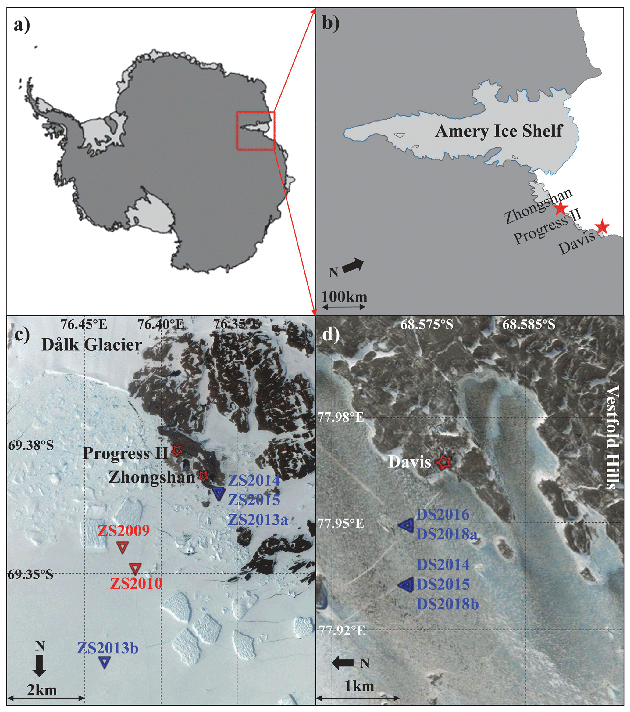
Figure 1Study area. (a) Antarctica with the red square indicating the study region. (b) The study region with the red stars indicating the Chinese Zhongshan Station (ZS), the Russian Progress II Station, and the Australian Davis Station (DS). (c) Close-up of ZS with the background showing a Landsat optical image obtained on 4 January 2011. (d) Close-up of DS with the background showing a Landsat optical image obtained on 13 October 2012. The red and blue triangles in panels (c) and (d) denote the CRREL-IMB and SIMBA deployment sites, respectively.
Here, we discuss the snow and LFI mass balance based on data collected by 11 IMBs deployed between 2009 and 2018 on LFI off ZS (6 buoys) and DS (5 buoys). The observations cover the ice seasons of 2009–2010, 2013–2016, and 2018 and form a contribution to the Antarctic Fast-Ice Network (AFIN) activities (Heil et al., 2011). The objectives of this study are (1) to quantify the seasonal, interannual, and spatial variability of the LFI snow and ice mass balance in the vicinity of these two stations, (2) to identify critical factors that are responsible for the LFI variability at local and regional scales, and (3) to determine the differences in the LFI thermodynamic processes in response to the local climate changes between the two stations.
2.1 Observation sites
Located on the eastern rim of Prydz Bay and affected by the same large-scale climate regime, ZS and DS (Fig. 1b) are approximately 110 km apart and experience similar atmospheric conditions (Streten, 1986). However, the wind forcing at ZS is characterized by dominant easterly katabatic winds, while the influence of katabatic flow at DS is less (Heil et al., 1996). The topography and bathymetry around ZS are relatively complex, with numerous small islands, grounded icebergs, and undulating submarine topographic features (Feng et al., 2008). The distribution and seasonal evolution of LFI off ZS are also affected by the small-scale Dålk Glacier, which enters the ocean with a frontal width of approximately 1 km (Chen et al., 2020). Glacial valleys and compressed terrain associated with the Dålk Glacier can strengthen the katabatic drainage and thus enhance the local wind force. In comparison, the water depths around DS are rather shallow and the offshore islands are sparse. With a similar annual cycle, the LFI at ZS and DS starts to form in early austral autumn (March) and finally breaks up during strong winds and/or high tides in austral summer (from mid-December to late January). The growth and expansion season of LFI in both regions can reach 10 months, which is much longer than its melting season of approximately 2–3 months (Heil, 2006; Lei et al., 2010). Occasionally, a small portion of LFI may survive through the summer within some small shielded narrow fjords near ZS (Tang et al., 2007; Zhao et al., 2017). However, there is little or no perennial ice in the LFI record at DS (Heil, 2006), which can be attributed to the difference in the coastal topography relative to that at ZS. Therefore, these two stations are ideal locations to examine the influence of differences in topographical and other local environmental variables on Antarctic LFI processes under similar atmospheric forcing.
2.2 IMBs and meteorological data
Two types of IMBs were used for observations: IMBs designed by the US Cold Regions Research and Engineering Laboratory (CRREL-IMB) and Snow and Ice Mass Balance Arrays (SIMBA) designed by the Scottish Association for Marine Science, Scotland. Technical details concerning CRREL-IMB and SIMBA are summarized in Table S1 of the Supplement and can be found in Richter-Menge et al. (2006) and Jackson et al. (2013), respectively. Data collected from two CRREL-IMBs and nine SIMBAs were used in this study. The details concerning the buoy deployments are summarized in Table 1.
Table 1Details concerning the ice mass balance buoy (IMB) deployment.
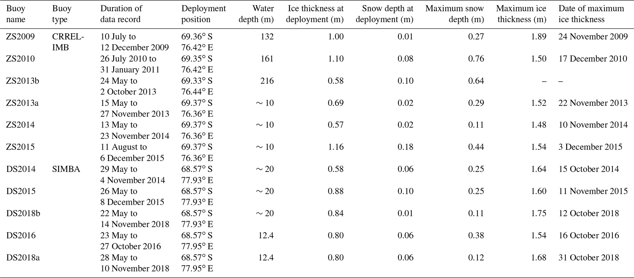
The buoys were named according to the deployment location and year. Because of safety concerns, all IMBs were deployed after late April when the ice thickness was greater than 0.50 m. The ZS2009, ZS2010, and ZS2013b deployment sites were approximately 3–6 km northeast of the shore with bathymetries deeper than 100 m (Fig. 1c); this avoids the shallow water and small islands near the shore and can be representative of LFI in the ZS offshore region. The ZS2013a and ZS2014, together with ZS2015, were deployed at sites approximately 100 m off the coastline northeast of ZS, with nearshore characteristics. The DS2016 and DS2018a were deployed approximately 1 km northwest off the coast of DS (Fig. 1d); this is a regular LFI measurement site and defined as S1 in Heil (2006). The DS2014, DS2015, and DS2018b were deployed approximately 1.5 km northwest of DS. All the deployment sites were classified as first-year ice. To ensure that the borehole for the buoy deployment was fully refrozen, our analyses used only data obtained 10 d after deployment.
The hourly meteorological parameters of 1989–2018, including the near-surface (at altitudes of 18 m at ZS and of 13 m at DS) air pressure (AP), air temperature (AT), relative humidity (RH), and wind speed and direction (WS and WD), measured at the ZS and DS meteorological stations were used to characterize the local atmospheric forcing. Daily solid precipitation (SP) was measured intermittently at the Russian Progress II Station (approximately 1 km from ZS) and is available in the form of the snow-to-water equivalent (SWE) for 2009–2018.
2.3 Determinations of the snow depth and ice thickness
For the CRREL-IMBs, the interfaces between the air and the snow or ice (in the absence of snow), as well as between the ice and the water, were measured using acoustic sounders with an accuracy of ±0.01 m, from which the snow depth and ice thickness can be derived by assuming that the interface between the snow and the ice remains unchanged. Unfortunately, the data from the underwater acoustic sounder of ZS2009 were unavailable after 2 August 2009 because of a sensor failure. Thus, we estimated the ice thickness of ZS2009 based on the difference in the vertical temperature gradients between the ice and the water (e.g., Perovich and Elder, 2001). The estimation error may be up to 0.05 m because of the relatively large vertical interval of the sensors for this style of IMB. SIMBAs feature a heating mode that provides the temperature rise after pulsed heating (HT) of 30 and 120 s (Jackson et al., 2013). The snow depths and ice thicknesses for the SIMBAs were derived from the vertical profiles of the temperature and HT (Provost et al., 2017; Liao et al., 2018). The snow depth and ice thickness were validated using in situ borehole measurements during the buoy operation periods from 2013 to 2015 off ZS and DS, with sampling intervals ranging from 3 d to 1 month. Compared with in situ observations, the temperature-profile-based estimations provided high accuracies of 0.001 ± 0.044 m for the snow depth and 0.006 ± 0.03 m for the ice thickness. Note that the topmost temperature thermistor of ZS2014 was just placed on the snow–ice interface at deployment as a result of an inaccurate operation. In addition, the topmost thermistor of ZS2013b was submerged within the snow after 6 September 2013 because the accumulated snow was too thick. Since the snow depth could not be retrieved from the temperature profiles at these two sites, the in situ measurements were used instead.
Furthermore, the upper ice surface might shift vertically as a result of the formation of snow ice or superimposed ice (Jeffries et al., 1998). The ratio between the 30 and 120 s HTs can be used to discriminate materials with different heat-capacity regimes, especially snow and sea ice (Jackson et al., 2013). Consequently, the data can be used to identify the formation of snow ice or superimposed ice. On the basis of a manual inspection of the vertical profiles of the HT ratio, vertical shifts in the snow–ice interface were clearly observed in the ZS2013a and ZS2013b data (Fig. 2). At other sites with SIMBA deployment, there was no identifiable change in the snow–ice interface, suggesting the lack of snow ice or superimposed ice formation.
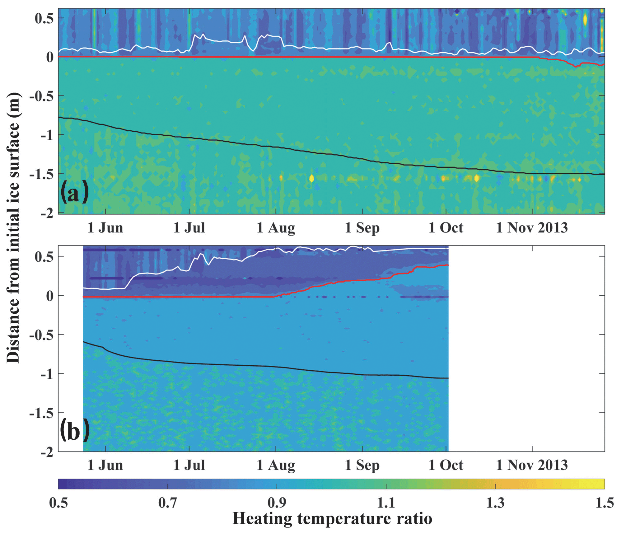
Figure 2Profiles of the pulsed heating (HT) ratio after 30 and 120 s observed by the (a) ZS2013a and (b) ZS2013b SIMBAs, with the white, red, and black lines denoting the snow surface, snow–ice interface, and ice bottom, respectively. The zero y value refers to the initial snow–ice interface at the buoy deployment.
To identify the probability of the occurrence of snow ice, the ice freeboard, Hf, for each IMB was estimated using Archimedes buoyancy principle (Provost et al., 2017):
where Hi and Hs are the ice and snow thicknesses, respectively, and ρi, ρs, and ρw are the densities of sea ice, snow, and seawater, with typical density values of 910, 330, and 1028 kg m−3, respectively (e.g., Lei et al., 2010). A negative ice freeboard is one of the most important indicators for the formation of snow ice (Rösel et al., 2018).
2.4 Heat fluxes through the ice and at the ice base
At the ice base, the heat fluxes satisfy the balance:
where Fc is the conductive heat flux through the basal ice layer, Fl is the equivalent latent heat flux caused by ice freezing or melting, Fs is the specific heat flux caused by ice warming or cooling, and Fw is the oceanic heat flux. The upward (Fc and Fw), melting (Fl), and warming (Fs) heat fluxes are defined as positive. Fl and Fs are calculated based on the ice growth rate and the temporal changes in the ice temperature, respectively. Fc was estimated based on the vertical ice temperature gradient (Lei et al., 2010). The latent heat, specific heat, and thermal conductivity of sea ice used to estimate these heat fluxes are functions of its temperature and salinity (Ono, 1967; Pringle et al., 2006). To calculate Fc and reduce the influence of the nonlinear vertical temperature gradient in the ice basal skeleton layer, we define the reference basal layer as the layer 0.12–0.24 m above the ice base (Lei et al., 2010). In our calculations, we linearly interpolated the temperatures of the CRREL-IMBs to an interval of 0.02 m, consistent with the measurements of the SIMBAs. The density and salinity of the newly-formed basal ice layer were set to 910 kg m−3 and 8, respectively. The 15 d moving average data were used for the estimations of the heat fluxes to reduce the uncertainties in the measurements. We quantified these heat fluxes to characterize their respective contributions to the ice basal growth.
The conductive heat flux was also estimated for each layer of 0.12 m throughout the entire ice column to assess the delayed response of the ice cooling or warming and the ice basal growth to the changes in atmospheric forcing. To calculate the conductive heat fluxes, we used a sea ice density of 910 kg m−3 and an ice salinity of 3 for the top 0.5 m section (considering its desalination; e.g., Lei et al., 2010) and 5 for the section below 0.5 m.
2.5 Assessing the effects of the snow cover, AT anomaly, and oceanic heat flux on the LFI growth
Under cold conditions, a linear vertical temperature change is adequate between the ice top surface at Ts and the base at the freezing point Tf; the thermodynamic ice growth can be approximately estimated by equating the latent heat removed to the vertical heat conduction upward through the ice to the colder air above (Stefan, 1891). Considering the contributions of the oceanic heat flux, the revised Stefan law (Leppäranta, 1993) is given as
where is the ice growth rate, ρi is the density of sea ice, Li and ki are the latent heat and thermal conductivity of sea ice, respectively, and is the vertical ice temperature gradient. With an initial ice thickness H0, the analytical solution for the ice thickness Hi can be estimated as
where
Here, θ is the integral of the negative ice surface temperature Ts below the freezing point Tf (here, defined as −1.9 ∘C) over time.
To identify the impact of snow cover on the LFI mass balance from the perspective of thermal insulation effect, we used the AT obtained from the year of observation (AT_obs) instead of Ts for the LFI thickness calculation; consequently, θ is equivalent to freezing degree days (FDDs). To identify the influence of the AT anomaly during the buoy operation years on the LFI mass balance, the LFI growth derived using the revised Stefan analytical model forced by AT_obs was compared with that forced by the 1989–2018 average AT (AT_mean). To assess the effect of the oceanic heat flux on the LFI growth, we compared the evolutions of the ice thickness from the beginning of the observations to the end of October, estimated using Eq. (4) with those estimated ignoring the oceanic heat flux. In these comparative estimations, we used the AT_obs instead of Ts to ensure consistency.
3.1 Atmospheric conditions
Compared with the buoy-observed data over 10 years, the mean biases of the AT measured at the ZS and DS onshore weather stations were very small, with values of 0.4 ± 1.6 and 0.3 ± 2.2 K, respectively. Therefore, we used the meteorological station data for the following analysis of the atmospheric conditions to identify the anomalies in the buoy operation years compared with the climatology. Because the meteorological data from ZS were available since 1989, we used the data from 1989–2018 to identify the anomalies for both stations.
At ZS, during 2009–2018, the annual mean AT was −10.2 ∘C, with the highest value observed in 2009 (−9.3 ∘C) and the lowest observed in 2015 (−11.3 ∘C); this was comparable to the 1989–2018 climatology (−10.0 ∘C) (Table 2 and Fig. 3a). The AT from May to September averaged for each year, defined as the mean AT of the LFI rapid growing season, was −15.9 ∘C at ZS during 2009–2018 (Fig. 3a). The annual mean WS was 6.6 m s−1, 73 % of which accounts for wind from the east-northeast–east-southeast direction (Fig. 3d). Under the influence of persistent cold dry katabatic winds, the annual accumulative SWE of the SP was relatively low, with an average of 192.8 ± 59.9 mm during 2009–2018. The annual SP varied greatly from year to year, with larger amounts of precipitation observed in 2013 (239.3 mm) and 2015 (230.8 mm) and smaller amounts in 2009 (124.5 mm) and 2018 (153.0 mm).

Figure 3Atmospheric parameters measured at ZS (red) and DS (black) from 2009 to 2018: (a) annual mean air temperature (AT; solid line, left axis) and mean AT of the LFI rapid growing season (dashed line, right axis), (b) monthly mean AT (solid line, left axis) and AT anomaly (shaded area, right axis), (c) monthly accumulative SWE of SP obtained from the Russian Progress II Station, and (d) frequency distribution of wind speed (WS) and wind direction (WD).
During 2009–2018, the winter and summer AT values at DS were 0.7 ∘C colder and 0.5 ∘C warmer, respectively, than those at ZS (Fig. 3b). The difference between the mean AT of the LFI rapid growing season at the two stations (DS−ZS) was −0.6 ∘C on average. During 2009–2018, the lowest (highest) AT of −11.4 ∘C (−9.0 ∘C) was observed in 2015 (2018) at DS, with large AT anomalies primarily occurring between May and September (Fig. 3b) associated with atmospheric cyclonic systems. On the edge of the low-lying Vestfold Hills, DS experiences relatively mild wind conditions, with an annual mean wind speed of 6.1 m s−1. The occurrence of winds with speeds larger than 8 m s−1, which were defined as the threshold for drifting snow (Schmidt, 1981), was 23 % at DS, much smaller than that at ZS (35 %). With less influence of dry katabatic winds, the long-term mean of annual accumulative SWE of the SP at DS was 231 mm (Heil, 2006), approximately 40 mm larger than that at ZS in 2009–2018.
Table 2Statistics of the principal meteorological parameters at ZS and DS.
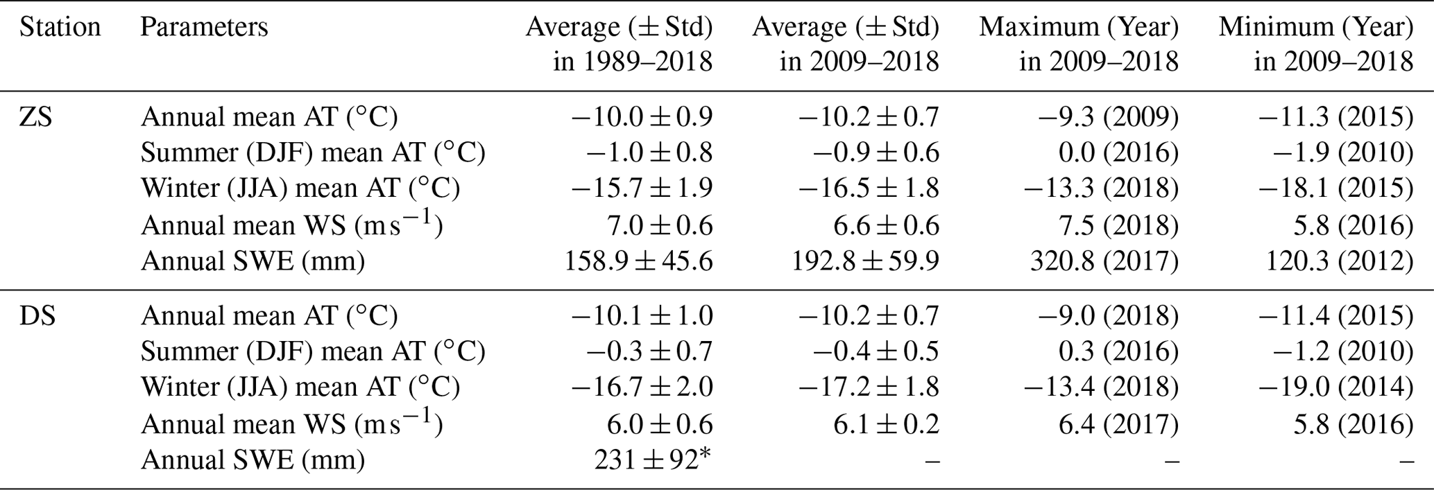
Note: ∗ From Heil (2006). “–” indicates that the data were unavailable.
3.2 Snow and sea ice mass balance at ZS
At the buoy deployments near ZS, the snow cover was relatively thin in mid- and late May (Fig. 4a), with a depth of less than 0.10 m. Most of the high snow-accumulation rates were synchronous with large SP amounts (Fig. 3c). The most noticeable snow accumulation was observed at ZS2010, with the snow depth increasing from 0.40 to 0.73 m during 13 to 15 September 2010. In this period, two snowfall events occurred with the SWE of the SP being 26.1 mm, contributing to 0.11 m of on-site snow accumulation. Considering that the ZS2010 buoy was deployed in an area with plethora of grounded icebergs (Fig. 1c), the persistent east-northeast wind after the first snowfall event and the sheltering effect of the grounded icebergs and growlers may have promoted snow accumulation on their lee sides and led to the additional increase in the snow accumulation in these locations. After the second snowfall event, strong winds occurred with speeds reaching 20.6 m s−1 and a directional change from east-northeast to east. Therefore, the accumulated snow was prone to being blown away. Consequently, the snow depth sharply decreased to 0.48 m by 17 September 2010. It is clearly shown that blowing snow played a vital role in the snow redistribution, especially for the fresh non-compacted snow, and contributed to the dramatic variations in the snow depth over the LFI off ZS.
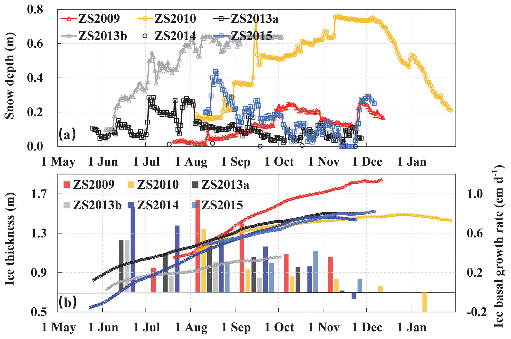
Figure 4Seasonal evolution of (a) the snow depth and (b) the ice thickness (lines, left axis) off ZS derived from CRREL-IMB and SIMBA observations, with the bars in panel (b) denoting the monthly ice basal growth rates (right axis). The snow depth of ZS2014 was obtained from in situ measurements and showed as blue circles.
The snow depths at all of the measurement sites reached their annual maximums from late June to late November (Fig. 4a), which was a very long temporal span, indicating that nearly all annual maximums were related to episodic synoptic events. At the inshore sites (ZS2013a, ZS2014, and ZS2015), the annual maximum snow depth ranged between 0.11 and 0.44 m. Meanwhile, at the offshore sites (ZS2009, ZS2010, and ZS2013b), the maximum snow depth was relatively large, with values reaching 0.27 (ZS2009), 0.76 (ZS2010), and 0.64 m (ZS2013b). Compared with the inshore sites, the relatively weak wind forcing and the shielding effect of the local topography of the small islands and grounded icebergs were likely related to the thicker snow cover at the offshore sites. With the lower occurrence frequency of snowfall in spring, except for occasional cases (e.g., in late November in 2009 and 2015), the snow depth gradually decreased with the processes of surface sublimation and/or snow compaction. When the air temperature rose above 0 ∘C after December, the snow depth dropped sharply; this can be clearly observed at nearly all buoy deployment sites. As a result of the relatively thin snow cover in the late ice growing season at ZS2014, ice surface melt started in mid-November at this site, much earlier than at the other sites.
The growth and expansion of LFI around ZS are not a continuous process. In general, the onset of a continuous LFI cover occurs in early to mid-March (Lei et al., 2010). After repetitive processes of ice formation, breakup, and reformation during the early freezing season as a result of wind forcing and/or ocean dynamics, the LFI cover around ZS becomes relatively stable from April onward. From our observations, three growth stages were identified based on the LFI thermodynamic growth process (Fig. 4b). From May to September, the LFI was in a rapid growth stage, with an average monthly ice basal growth rate of 0.5 ± 0.2 cm d−1. The maximum monthly ice basal growth rate occurred in August 2009, reaching 0.9 cm d−1. During the period of October–November, with the thickening of the ice cover and the increase in AT, the ice growth gradually decelerated and ceased, suggesting a steady growth stage with a monthly basal growth rate of 0.2 ± 0.2 cm d−1. The annual maximum ice thickness was observed by the end of this stage (i.e., mostly in late November), with a value of 1.59 ± 0.17 m obtained from five sites measured in 5 years (Table 1). Note that the annual maximum ice thickness at ZS2013b could not be obtained because the observation was invalidated before the ice thickness reached its annual maximum. After a state of thermal equilibrium, the LFI near ZS entered a melt stage from late November until the ice breakup occurred in late December or early January (Lei et al., 2010).
The evolution of the LFI mass balance also exhibited large spatial variations. Approximately 6 km apart, the ZS2013a and ZS2013b sites experienced nearly the same atmospheric conditions; however, the total ice basal growths at these two sites revealed large differences, with values of 0.52 and 0.33 m from 3 June to 1 October, equivalent to latent heat fluxes of 10.2 and 6.5 W m−2, respectively. Located within a typical distance from the shore (6–15 km) where continental winds diminish and drifting snow tends to accumulate (Fedotov et al., 1998), significant amounts of accumulated snow were observed at ZS2013b. The snow cover at ZS2013b reached 0.30 m in mid-June, approximately 0.20 m thicker than that at ZS2013a, which efficiently insulated the LFI from the cold atmosphere and substantially reduced its basal growth. However, the snow depth at ZS2013a decreased rapidly and maintained a value of approximately 0.10 m after reaching its annual maximum (0.29 m) in early July. By the end of the observation period in early October 2013, the LFI thickness at ZS2013b was 1.06 m, much smaller than the thickness (1.42 m) observed at the same time by ZS2013a.
3.3 Snow and sea ice mass balance at DS
The seasonal evolution of snow depth at DS remained rather smooth and the amplitude of short-term fluctuations were much smaller compared with those at ZS because of the relatively open terrain and mild wind conditions (Figs. 4a and 5a). At deployment in late May, the snow depth around DS ranged between 0.01 and 0.10 m. Snow accumulated gradually from May to July. The annual maximum snow depths all occurred in winter (from June to August), with values varying from 0.11 to 0.38 m. From then onward, the snow depth gradually decreased until the end of the measurements in December.

From early or mid-March, LFI formed around DS and a stable cover was presented by April. The annual maximum ice thickness was observed between mid-October and mid-November (Table 2), with the mean value obtained from five IMBs being 1.64 ± 0.08 m, which was slightly larger than the mean value obtained at ZS (1.59 ± 0.17 m). Entering the melting stage, final LFI breakup was generally observed from mid-December to February and was typically associated with passing cyclonic activities (Heil, 2006).
IMB observations were made simultaneously on the LFI near DS and ZS during the two ice seasons of 2014 and 2015. The snow cover did not differ much between the two sites during the same year, except for variations related to several synoptic events. However, during the rapid ice growth stage from May to September, the LFI grew faster at DS with an ice basal growth rate of 0.6 ± 0.2 cm d−1, compared to 0.5 ± 0.2 cm d−1 at ZS (Figs. 4b and 5b). Correspondingly, the LFI thickness at DS2014 and DS2015 increased to 1.52 and 1.47 m, respectively, by the end of September, which were 0.15 and 0.13 m thicker than those at ZS2014 and ZS2015, respectively. This may be partly attributable to the relatively lower ATs at DS over this time (Fig. 3a). The FDDs at DS were 2189.5 and 2572.9 K d in 2014 and 2015, respectively, approximately 6.8 % and 2.4 % larger than those at ZS (2049.8 and 2513.4 K d, respectively). After September, with the increases in AT and ice thickness, the LFI at DS entered the steady growth stage; the maximum ice thickness at DS was observed approximately 20 d earlier than that at ZS (Table 1). Because of the relatively warm summer and the lack of shelter due to only few coastal islands and grounded icebergs, the LFI broke up off DS earlier than off ZS. There was an ice-free period of approximately 1 month in the vicinity of DS, which was longer than that of ZS by approximately 10–20 d (Heil, 2006; Lei et al., 2010).
3.4 Sea ice temperature profile and heat flux
As an example, Fig. 6 presents profiles of the snow and sea ice temperatures and the conductive heat flux through the LFI at ZS2013a. The conductive heat fluxes centered at depths of 0.12 m below the ice surface and 0.12 m above the ice bottom were used to indicate the surface and bottom layers of the ice column (Fig. 6c), respectively, which participate in the thermal balance with the snow and the ocean. Note that the thin layers (0.06 m) near the upper and lower boundaries of the ice layer are not considered here, primarily because these two thin layers have complex texture structures; that is, they are scattering layers similar to the snow at the top layer and the mush layer at the ice bottom.
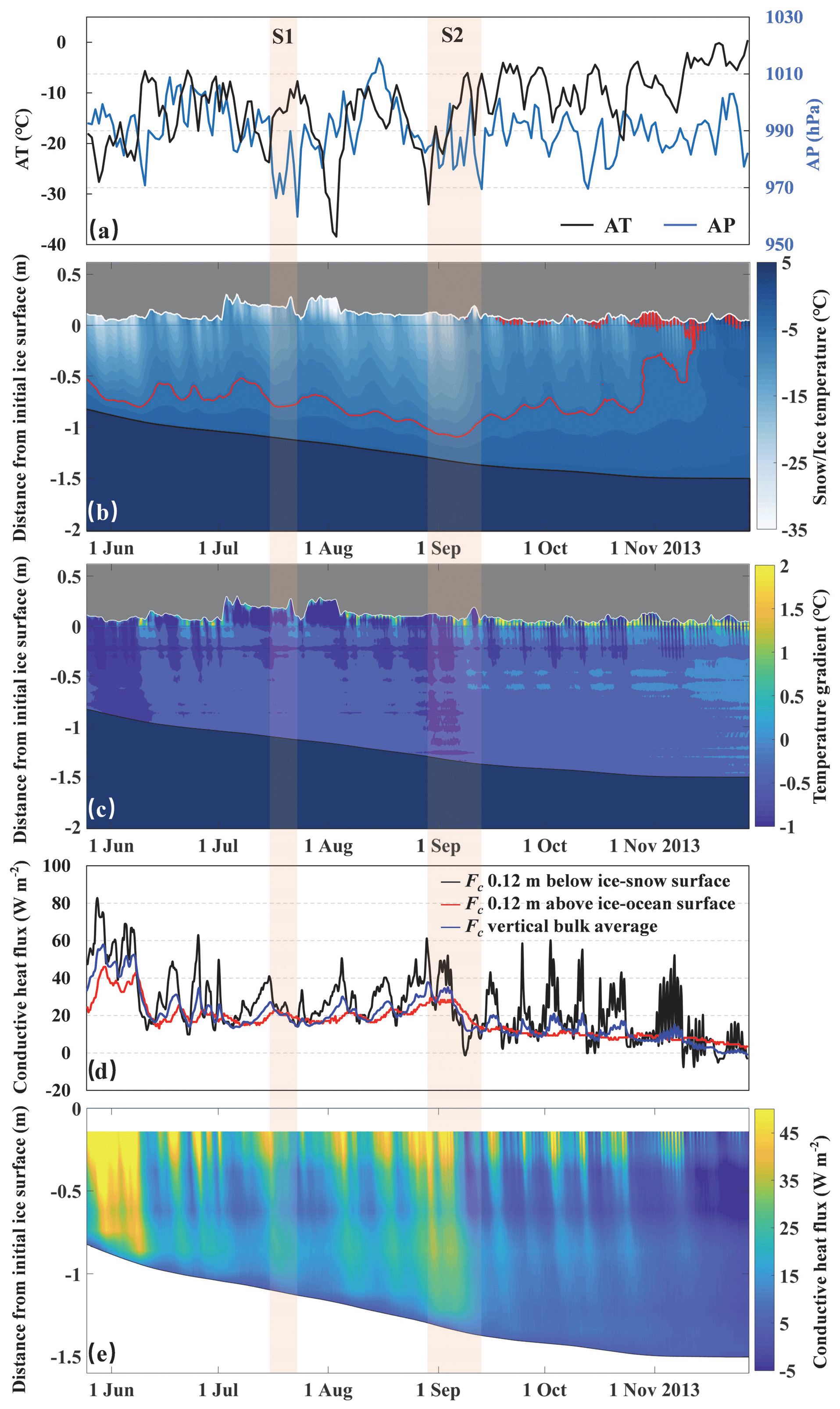
Figure 6(a) Time series of the AT and AP; (b) snow and sea ice temperatures, with the white, red, and black lines representing the snow surface, the −5 ∘C isotherm, and the ice bottom, respectively; (c) snow and sea ice temperature gradients; (d) conductive heat flux through the ice; and (e) conductive heat flux through the ice at ZS2013a. On the vertical axes of panels (b), (c), and (e), the zero line refers to the initial snow–ice interface. The shaded areas represent periods experiencing two typical warming events of S1 and S2.
During winter, when the study region was under the control of the Antarctic high-pressure atmospheric system, a rapid decrease in the temperatures occurred in the snow cover and upper layers of the ice in response to the decreasing AT (Fig. 6a and b). The variation range of the temperature at the snow–ice interface was only half of that of AT, from which the thermal insulation effect of a snow cover can be readily appreciated. The snow layer, with a smaller density and thermal conductivity, had an obviously larger temperature gradient compared with the ice. Conversely, episodic warming events occurred frequently in winter when low-pressure synoptic systems were in place. During these events (e.g., S1 and S2 shown in Fig. 6a), the temperature gradient in the snow layer became inverted, with the local temperature minimum occurring at the snow–ice interface or the top layer of the ice (Fig. 6c). With the sharp increase in AT and the thickening of the snow cover during these events, the conductive heat flux at the ice surface layer dropped dramatically by approximately 20 W m−2 within 3–5 d. The fluctuation of the conductive heat flux near the ice bottom was relatively smooth and revealed a temporal lag relative to that at the ice surface layer, which may be related to the buffering effect of ice layers and internal brine (Fig. 6d). This temporal lag was about 3 d in mid-July (S1) and reached 7 d by late August and early September (S2), changing the direction of the vertical heat conduction within the ice column (Fig. 6d). Beginning in spring, the diurnal signal in the temperature profile became increasingly pronounced at the top ice layers because of the increase in the incoming solar radiation and daily AT fluctuation. At that time, the bulk conductive heat flux through the entire ice column decreased to several W m−2 (Fig. 6d). After 10 November 2013, negative conductive heat flux occurred in the top ice layer at approximately 0.7 m (Fig. 6e); this was attributed to the temporal lag of the seasonal warming of the lower ice layers relative to the increase in AT as a result of the heat storage capacity of the brine within the ice. At this time, a downward conduction of the heat flux into the middle layer of the ice was observed, promoting further interior melting of the ice. Therefore, an internal melting gap layer was often observed approximately 0.10 m to tens of centimeters below the ice surface at ZS; this weakened the ice layer and promoted the breaking up of the LFI (Zhao et al., 2022).
To assess the relative contributions of each component of the heat fluxes at the ice bottom to the LFI growth, the basal heat flux components at each buoy site were compared (Fig. 7). The potential error in the estimation of heat fluxes arises from individual uncertainty in the ice salinity, temperature, density, and thickness, which has been estimated about 1–2 W m−2 (Lei et al., 2014). Throughout the entire observation period, because the temperature at the ice base was nearly constant, Fs was always relatively small. The basal ice growth was primarily regulated by Fc and Fw. Fc contributed approximately 50 % to the basal ice energy balance (Fig. 7i and j). For the nearshore (ZS2013a) and offshore (ZS2013b) sites around ZS (Fig. 7a and b), the maximum Fc occurred on 3 June, with a value of 45.2 W m−2 at ZS2013b, approximately 8.0 W m−2 larger than that at ZS2013a. At this time, the basal ice growth rate at ZS2013b was 0.7 cm d−1, comparable to the rate at ZS2013a; this is primarily attributable to the difference in the oceanic heat fluxes under the ice between two sites. During the initial freezing period with a large ice growth rate, the surface seawater was densified by brine rejection from sea ice which drove vertical mixing. The coastal water at ZS2013a is shallow (<10 m) and is expected to be entirely mixed. Approximately 6 km offshore, the water depth at ZS2013b is up to 216 m. Therefore, the potential upward entrainment of warmer deep water at this site likely resulted in a higher value of the ocean heat flux (22.2 W m−2) and provided a thermal constraint on the LFI growth. After mid-June 2013, Fw at both the ZS2013a and ZS2013b sites dropped to less than 10 W m−2. Meanwhile, with the increasing snow depth, Fc at the ice basal layer of ZS2013b decreased sharply to approximately half that of ZS2013a. Correspondingly, the basal ice growth rate at ZS2013b decreased to 0.3 cm d−1, 60 % of the rate at ZS2013a (0.5 cm d−1).
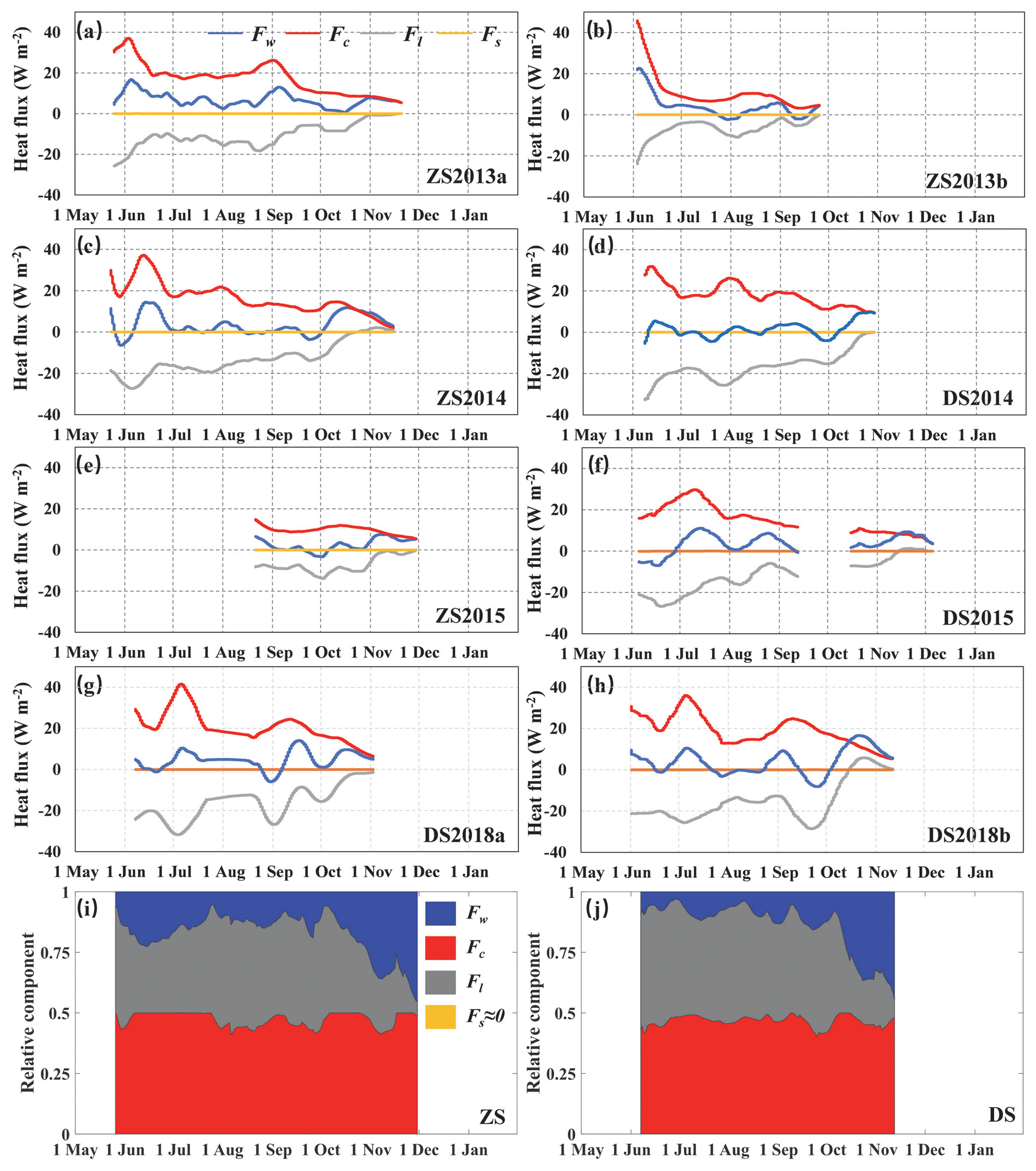
Figure 7(a–h) Heat flux components obtained from the IMB observations at different sites, with the two panels in each row obtained in the same year, and the averaged relative contributions to the total heat balance at ice bottom of the (i) six sites at ZS and (j) five sites at DS.
When compared, the measurements obtained from the coastal sites near ZS and DS during the same year (ZS2014 versus DS2014, as shown in Fig. 7c and d; and ZS2015 versus DS2015, as shown in Fig. 7e and f), Fc revealed a similar seasonal pattern for the two sites, with the largest value observed in June and then decreasing gradually until the end of the observations by late October in 2014 or late November in 2015. The mean Fc values from June to October 2014 and from August to November 2015 were comparable in the same year between the two sites, with values of 17.0 and 10.8 W m−2 at ZS and 16.5 and 10.7 W m−2 at DS, respectively. Meanwhile, the mean Fw under the LFI from June to September (3.2 W m−2), during the stage of rapid ice growth, and its contribution to the basal ice energy balance (14.1 %) at ZS were much larger than those at DS (0.7 W m−2 and 8.8 %, respectively). This relatively large oceanic heat flux at ZS which reduced the ice basal growth, together with the relatively small mean Fc, led to an annual maximum LFI thickness that was thinner than at DS (1.48 m versus 1.64 m in 2014 and 1.54 m versus 1.60 m in 2015). Approximately 500 m apart, DS2018a and DS2018b had nearly the same snow depth and ice thickness evolution, resulting in close conductive heat fluxes through the ice (Fig. 7g and h). The Fw at these two sites showed a slight difference after late August, with the minimum occurring in early September at DS2018a and in late September at DS2018b. Further away from the shore, the Fw at DS2018b continued to increase from the minimum of −8.2 W m−2 in 26 September to 15.0 W m−2 by mid-October. Note that the temporary negative value of Fw can be partly attributable to the potential estimation uncertainty, given that the nearest glacier, Søsdal Glacier, is about 12 km south of DS. To clarify whether the negative Fw was associated with supercooled glacial meltwater, simultaneous observation of under-ice turbulence and detailed measurement of sea ice physical parameters are recommended in the future. Combined with the decreased Fc, this resulted in the earlier onset (17 October) of ice basal melt at DS2018b than at DS2018a (3 November). Note that the relative contributions of each component to the total heat balance at the ice bottom shown in Fig. 7i and j were obtained from multi-site measurements, which can be considered to be the average state of the LFI heat balance at the two stations and crucial information for the validation of regional LFI numerical simulations.
4.1 Comparison with early studies
The mass balance measurements of the LFI around ZS and DS given in this study (Table 1) were compared with those obtained in previous studies (Table 3); the results suggest a stable long-term condition of the LFI mass balance at both stations in eastern Prydz Bay. For a site close to the coast near ZS (site SIP in Table 3), with data from 6 years (2006 and 2012–2016), large interannual variability in the annual maximum ice thickness and its occurrence (from early November to early December) could be identified. The mean annual maximum LFI thickness was 1.62 ± 0.14 m (Tables 1 and 3), with the maximum observed in 2016 (1.82 m) and the minimum in 2015 (1.49 m). The obvious discrepancy in the snow accumulation between these 2 consecutive years was the main factor contributing to the difference in the annual maximum ice thickness. Similarly, at DS, combining the data used in this study (DS2016 and DS2018a) with the 26-year data from the period of 1957–2009 obtained at the same site (site S1 in Table 3, Heil, 2006; Heil et al., 2011), the annual maximum LFI thickness at DS did not reveal a significant trend and showed large year-to-year variability. In 2016 and 2018, the annual maximum ice thickness was observed in mid- to late October, which was relatively early compared to the 1957–2009 average (around 10 November). Our results did not follow the delayed trend obtained for the period of 1957–2009 by Heil et al. (2011). This suggests that this trend is likely not robust. At the Troll/Fimbulisen site (2005–2010; Heil et al., 2011) and the Atka Bay site (2010–2018; Arndt et al., 2020) in the eastern Weddell Sea and the McMurdo Sound “sea ice runaway” site in the Ross Sea (1986–2013; Kim et al., 2018), no significant trends were identified for either the annual maximum snow depth or the LFI thickness. This suggests that the circum-Antarctica LFI mass balance has likely been in a relatively stable state over the past few decades. This can partly be associated with the ambiguous trends for the AT at these stations. For example, the trends of increasing AT at DS, Troll/Fimbulisen, and Neumayer (Weddell Sea) were insignificant, and the trend at McMurdo Sound (Ross Sea) was significant only in spring with a confidence level of 0.10 (Turner et al., 2019). In addition, the role of snow accumulation complicates the response of the LFI to local climate change. The modeling result suggests a delicately balanced Antarctic snow–sea ice system, where either a decrease or an increase in the snowfall rates or snow redistribution due to blowing snow could lead to an increase in the ice thickness because of the regulation of the basal freezing and the formation of snow ice or superimposed ice (Fichefet and Morales Maqueda, 1999; Powell et al., 2005).
Table 3Summaries of previous studies on the landfast ice (LFI) mass balance around ZS and DS.
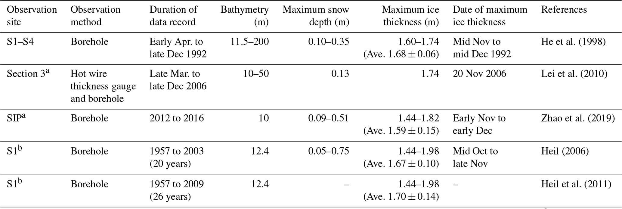
Note: a The locations of the site closest to the coast in Section 3 (Lei et al., 2010) and site SIP (Zhao et al., 2019) are the same as those of ZS2013a, ZS2014, and ZS2015. b The location of site S1 (Heil, 2006; Heil et al., 2011) is the same as that of DS2016 and DS2018a.
The LFI mass balance observations were made at individual sites. Thus, to derive a clear temporal trend of the LFI mass balance, it requires years of measurements located at exactly the same location with standard techniques. The measurement locations might influence the results due to its strong spatial dependence of the LFI mass balance even at a 1 km scale (Lei et al., 2010). Therefore, the differences in the observation sites and methods by the studies given in Table 3 also affect our evaluation results. In contrast to the unclear trend for the LFI mass balance, some statistically significant trends were found for the LFI extent and some timings of the LFI season for a larger-scale study. Compared with 3 decades ago, the maximum LFI area around Antarctica has decreased by approximately 10 % (Fedotov et al., 1998; Li et al., 2020); this overall decrease also occurred during the period from 2000 to 2018 (the length of the data record; Fraser et al., 2021). At a more local scale, a trend toward a delayed LFI breakout date and an increased LFI duration was identified over the period of 1969–2003 in the DS region of Prydz Bay (Heil, 2006) and over the period of 1978–2015 in McMurdo Sound of the Ross Sea (Kim et al., 2018). Note that the LFI in different regions may respond to changes of external forcing in different ways and that the spatial scales and local geographical environment provide key influence to the responding patterns, which may lead to inconsistent change trends (Fraser et al., 2021). For example, the final breakout date of the Antarctic LFI is more dependent on the dynamic nearshore processes, while the LFI extent is more dependent on the dynamic processes close to the open water. Conversely, the LFI mass balance in coastal regions depends more on local thermodynamic processes but is also affected by local small-scale dynamic processes, such as snow blowing, as revealed in this study. Therefore, to thoroughly understand the complex regional patterns of the changes in the Antarctic coastal LFI, a sustained and expanded LFI observing network with unified observation standards is essential; this includes monitoring of the sea ice geophysical variables, physical parameters of the atmospheric and oceanic boundary layers, as well as the dynamics of nearby cryospheric elements, such as changes in the iceberg distribution, the fronts of ice shelves, glaciers, and ice tongues.
4.2 Dominant factors for the LFI thermodynamic mass balance
In general, dynamic processes are mostly limited during the early freezing season for the Antarctic LFI. Once a solid ice cover forms, the subsequent growth of the LFI is primarily determined by thermodynamic processes that occur at the base of the ice as the heat is conducted upward and lost to the surface atmosphere. Therefore, the importance of the thermal effect of the snow depends on the thickness ratio between the snow and the ice. When removing the contributions of the snow layer by using AT_obs instead of Ts for the ice thickness calculation based on the analysis model, the simulated LFI thicknesses increased significantly at DS2014, DS2015, and DS2016 (Fig. 8g–i, respectively). Such a significant increase was not found in 2018, which is attributable to the observed thin snow cover of less than 0.10 m during most of the ice season at DS. Around ZS, when the effect of snow was not considered, the largest increase in the simulated LFI thickness was up to 0.35 m (or 33.0 %) at ZS2013b, corresponding to the highest thickness ratio of snow and ice at this site. However, even though the snow cover was relatively thick at ZS2010, the discrepancy between the simulated (without snow) and observed LFI thicknesses in early October was relatively small (0.24 m or 17.4 %); this was partly because the accumulation of snow mostly occurred in spring when the ice was entering the end of the growth period. During this stage with relatively thick ice, the effect of the snow became less important in reducing the ice growth rate (e.g., Merkouriadi et al., 2020).
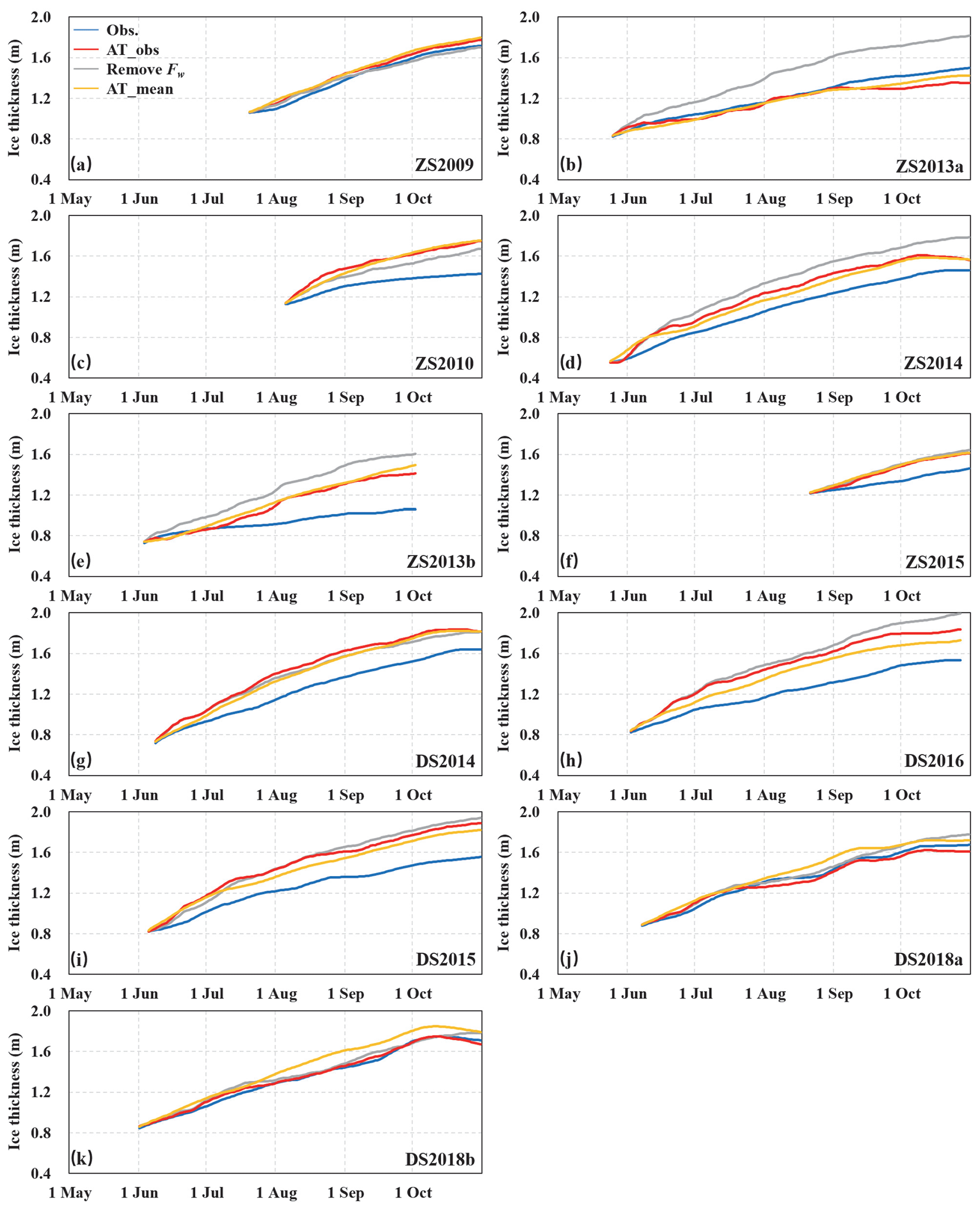
Figure 8LFI thicknesses observed by the buoys (blue line) and calculated ignoring the oceanic heat flux (gray line), using AT_obs (red line) and AT_mean (yellow line).
The sensitivity of the LFI mass balance to the AT anomaly is shown in Fig. 8. At DS, the discrepancies between the ice thickness estimated using AT_obs and that estimated using AT_mean ranged from −0.12 m at DS2018b to 0.11 m at DS2016 by the end of October because of the anomalously warm and cold winters in 2018 and 2016, respectively. The AT anomaly appears to have a larger impact on the LFI thickness at DS (4.3 % on average) than that at ZS (2.0 % on average). This difference indicates that the LFI at ZS was more influenced by other factors, such as the oceanic heat flux and the surface atmosphere–ice heat exchange associated with katabatic wind, compared to that at DS. During the same season, the difference between the estimated ice thicknesses using AT_obs and AT_mean was larger at ZS2013b and DS2018b with thinner ice thicknesses than at ZS2013a and DS2018a, respectively, which indicated that the AT anomalies are more sensitive with thin ice because of its weak thermal inertia (e.g., Lei et al., 2018). To assess the influence of climate change on the mass balance of Antarctic LFI, the seasonality of climate change should be considered because of the large seasonal differences in the response of sea ice growth to the AT anomaly.
Comparing the calculation results when considering or ignoring the oceanic heat flux in the analysis model, we found that oceanic forcing appears to exert a larger influence on the mass balance of the LFI near ZS than near DS (Fig. 8), which is also demonstrated by the difference in their relative contributions to the ice basal heat balance as shown in Fig. 7i and j. It was almost impossible for deep warm water to intrude into the coastal region around DS because of the shallow water depth, which led to low value and contribution to the LFI mass balance of oceanic heat flux. The averaged oceanic heat flux at DS was estimated to be 1.6 W m−2 during the period of June–October for the years from 2014 to 2018, which was comparable to the value (1.4 W m−2) obtained from 1980 to 1985 (Heil et al., 1996). After removing the oceanic heat flux component in the analysis model, the simulated ice thicknesses at the buoy sites near DS increased by 5.7 % on average by the end of October. Correspondingly, at ZS, the simulated ice thicknesses increased at many of the measurement sites when parameterizing Fw to zero, with the largest increase being 0.46 m (or 34.1 %) obtained at ZS2013a (Fig. 8b). However, ZS2009 and ZS2010 were two exceptions, with the simulated ice thicknesses at both sites decreasing by 0.07 m after removing the contributions of the oceanic heat flux (Fig. 8a and c). Located within an area of grounded icebergs that have been calved from Dålk Glacier (Fig. 1c), the seawater at a depth of 2 m at both sites was colder than the freezing point from July to October, with an average temperature of −2.0 ∘C. One possible explanation for the exceptions at ZS2009 and ZS2010 is that the seawater at these sites was likely supercooled and potentially related to the outflow of glacial meltwater, which resulted in a negative oceanic heat flux that was conducive to the LFI growth. Such a mechanism has been observed in LFI in the vicinity of several Antarctic ice shelves (e.g., Langhorne et al., 2015). To further understand the influence of supercooled glacial meltwater on the LFI mass balance, it is recommended to carry out simultaneous observations of the sea ice mass balance and the oceanography of the ocean stratification, heat content, and currents close to the glacial front. Isotopic analyses of the under-ice seawater are also helpful to identify the influence range of glacial meltwater in the LFI zone.
4.3 Flooding and snow ice formation
When the snow mass is sufficiently large, the ice surface submerges and slush is formed. Formation of snow ice depends on the evolution of the ice freeboard and ice permeability (Eicken et al., 1994, 1995). At our study sites, the estimated freeboards decreased as the snow accumulated and negative freeboards were identified at ZS2013b (Fig. 9a) and ZS2010 (Fig. 9c), suggesting the possibility of flooding. Ice surface flooding is controlled by upward brine percolation when the permeability of an ice layer reaches a threshold (Golden et al., 1998) or through macroscopic fractures when the ice surface is depressed because of local ice deformation (Lei et al., 2022). Seasonally, ice bulk temperatures usually reach the critical temperature of −5 ∘C around early November, which would effectively enhance the ice permeability. At ZS2013b, a snow storm occurred in early July and its resultant loading pushed the snow–ice interface below sea level (Fig. 9a). The impermeable layer, defined by temperatures below −5.0 ∘C, was warmed, caused by the AT increase during the storm and the LFI layer became permeable. Flooding occurred and the slushy layer refroze during the subsequent cold period forming snow ice. The obvious flooding event occurred in late August and lasted for approximately half a month. The upward shifting of the snow–ice interface by approximately 0.20 m could be observed clearly by the SIMBA HT ratio profile (Fig. 2b). Until the end of the observation in early October, the contribution of snow ice to the LFI mass balance reached 27 % (0.40 m) at ZS2013b. This proportion of snow ice was comparable to the results from previous studies of the LFI around ZS. On the basis of the ice core samples collected from the Nella Fjord close to ZS, Tang et al. (2007) found that the regional average proportion of snow ice varied from 8 % to 38 % by the end of the ice growth season in late January 2003. Using a sea ice thermodynamic model, Zhao et al. (2019) estimated that snow ice contributed to 4 %–23 % of the total maximum ice thickness for the LFI off ZS in 2012. Similar to ZS2013b, snow ice formation was very likely to occur at ZS2010 after mid-November, during a period when the snow–ice interface was approximately 6 cm below the sea level and the ice layer became permeable (Fig. 9d). The formation of snow ice has been simulated by Zhao et al. (2020) for LFI around ZS in 2015. However, neither the ice temperature nor the HT ratio profile at ZS2015 in our study shows signs of snow ice formation, which is likely because drifting snow was not considered in the sea ice model used by Zhao et al. (2020) and the simulated snow depth was much larger than the observed value at ZS2015.
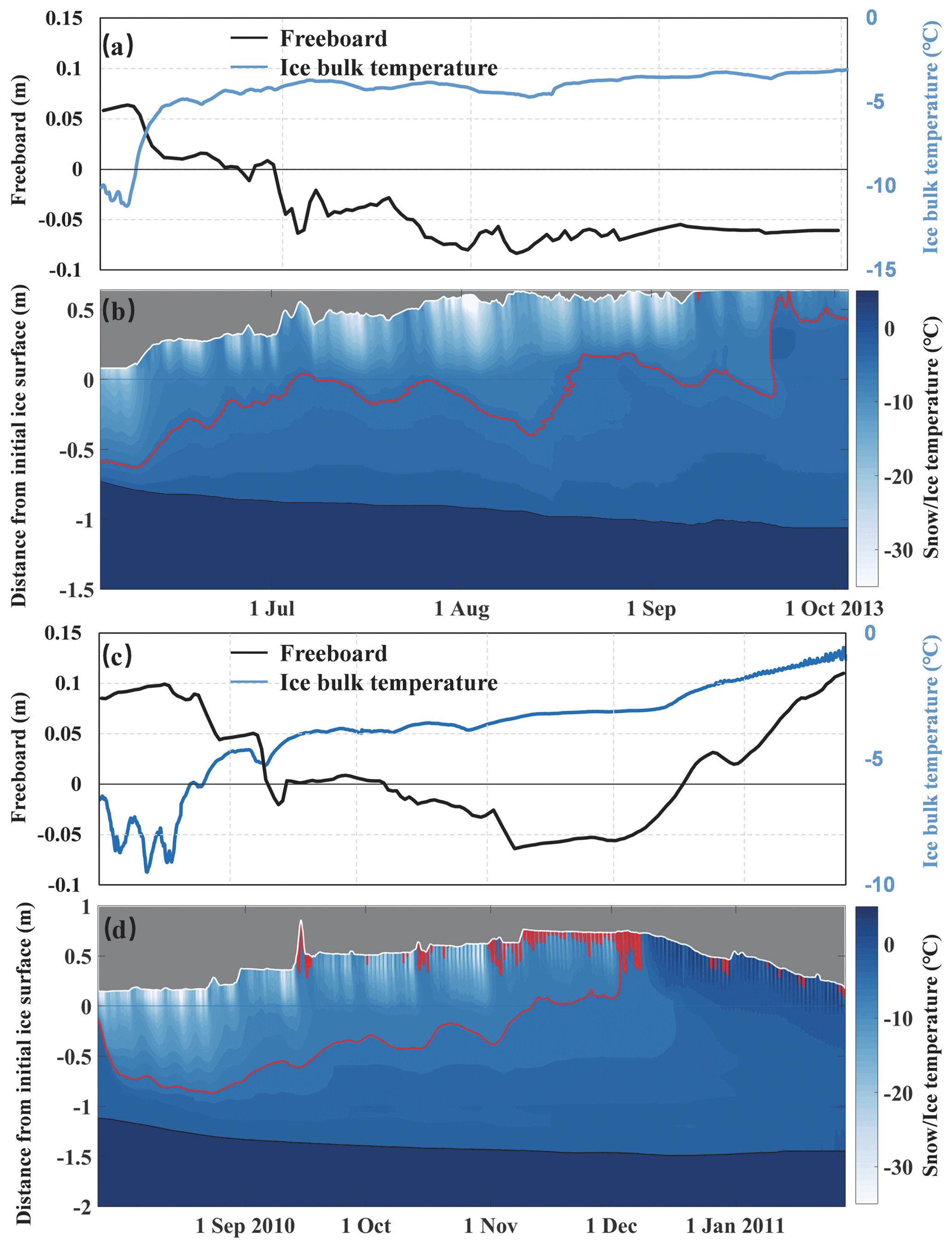
Figure 9Estimated sea ice freeboard and ice bulk temperature, and temperature contours in the snow and sea ice measured by (a and b) ZS2013b and (c and d) ZS2010. The white, red, and black lines in panels (b) and (d) represent the snow surface, the −5 ∘C isotherm, and the ice bottom, respectively. The y axis zero value denotes the initial snow-ice interface.
Our buoy data did not indicate any signs of the formation of snow ice over the LFI around DS, consistent with the results presented by Heil (2006). This was likely related to the relatively thin snow cover there. Therefore, the flooding and formation of snow ice in the LFI zone was not widespread, which differs from the drifting ice zone over the Southern Ocean (e.g., Eicken et al., 1994; Jeffries et al., 2001; Maksym and Markus, 2008). The dynamic deformation of LFI occurs only over a very small spatial range, together with the relatively small thickness ratio between the snow and the LFI compared with the drifting ice zone (e.g., Ozsoy-Cicek et al., 2013), which are likely the main reasons why flooding and snow ice formation over Antarctic LFI are not as widespread as in the drifting ice zone.
During spring and summer, Antarctic sea ice melts primarily from the bottom because of the relatively large oceanic heat flux, as well as the cool and windy surface conditions which prevent melt pond formation (Nicolaus et al., 2009; Arndt et al., 2021). Compared with the snow ice, the formation of superimposed ice was less extensive because of the lack of a supply of meltwater from surface. With the extensive surface thaw–refreeze cycles after mid-November in 2013, the downward shift of the snow–ice interface at ZS2013a provided evidence of the possibility of the formation of superimposed ice. At this site, the snow–ice interface was consistently above the water level, the snow meltwater percolated downward to the colder snow–ice interface where the superimposed ice formed. The superimposed ice formed in early November and lasted until 27 November at ZS2013a with a maximum thickness reaching 0.10 m (Fig. 2a). The contribution of the superimposed ice to the LFI mass balance in our study area can be considered to be weaker than that of the snow ice. However, the formation of superimposed ice can prevent the further downward infiltration of snow meltwater, which is expected to refreeze into ice plugs within the pores of the sea ice (Polashenski et al., 2012). Therefore, superimposed ice over the parental ice layer, even having a short life and a small thickness, would provide critical modification of the LFI thermodynamic processes.
Regional, seasonal, and interannual variations in the LFI mass balance in Prydz Bay, East Antarctica, were investigated using IMB data observed over 7 ice seasons during 2009–2010, 2013–2016, and 2018. The observations were obtained at two locations (ZS and DS) with a separation of 110 km and ranging between 100 m and 6 km from the shore. The differences of LFI mass balance and related atmospheric and marine environmental parameters between the two stations are summarized in Fig. 10, which are identified from this study and previous literature. A larger local spatial variability of the snow depth and ice thickness was observed over the LFI zone at ZS than at DS. The LFI around DS grew faster and reached a larger maximum ice thickness of 1.64 ± 0.08 m by mid-October to mid-November, which was approximately 20 d earlier than the occurrence of the maximum ice thickness around ZS (1.59 ± 0.17 m). We found significant interannual variability in the LFI mass balance at both the ZS and DS sites. This coincides with the LFI in the Weddell and Ross seas, where no clear trend of the LFI mass balance has been identified (Heil et al., 2011; Kim et al., 2018; Arndt et al., 2021).
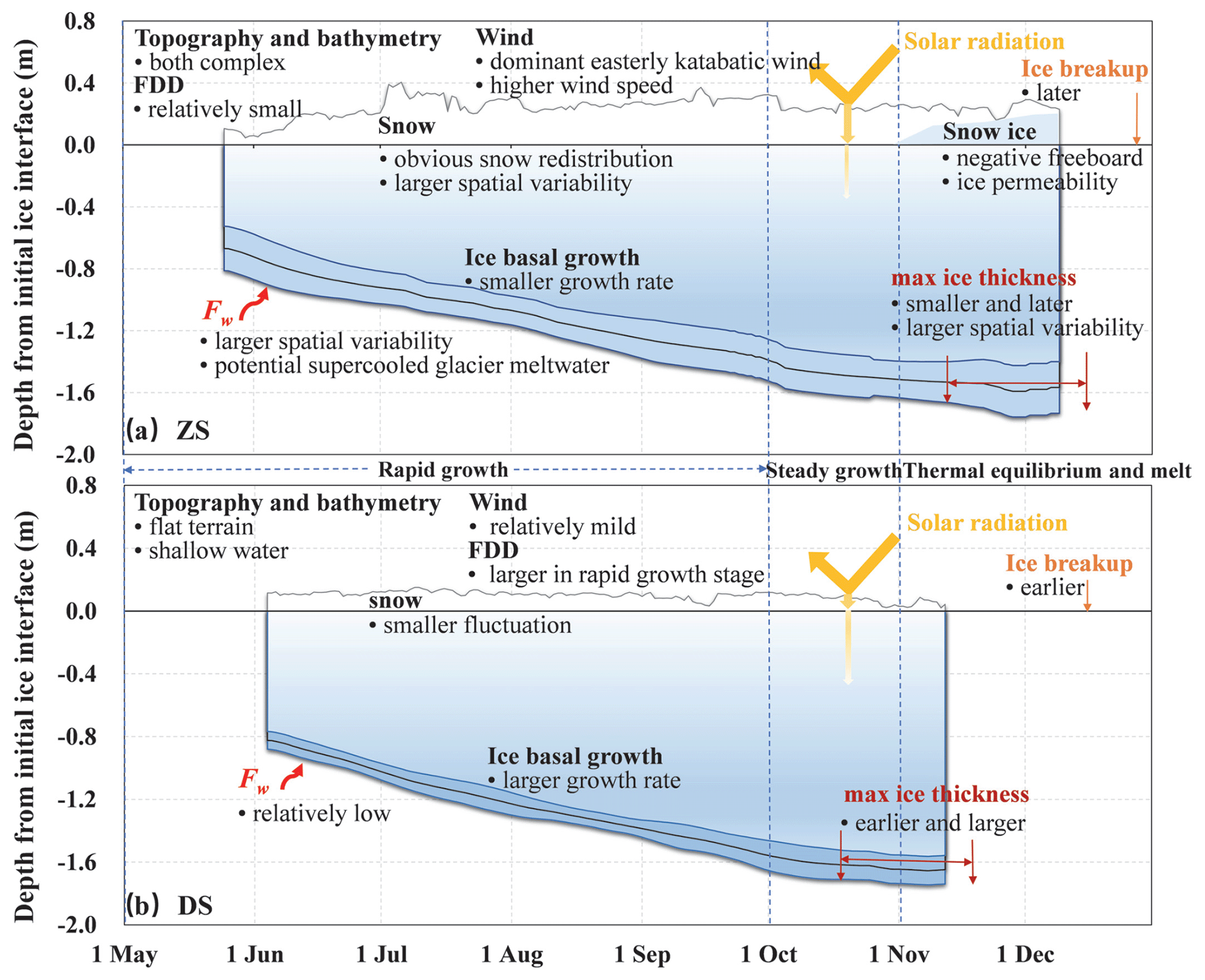
Figure 10Schematic diagram of the seasonal and interannual characteristics of LFI near ZS (a) and DS (b), with the critical factors that are responsible for the LFI variations. The gray, black, and blue lines represent the spatially averaged snow depth, LFI thickness, and the LFI thickness ± standard deviation, respectively.
The snow accumulation showed a distinct pattern between the ZS and DS sites. During the observation period, the maximum snow depth around ZS and DS had ranges of 0.11–0.76 and 0.11–0.38 m, respectively. This difference was partly due to local differences in the solid precipitation, as well as the distribution and morphology of the grounded icebergs associated with the wind regime, which played a critical role in the initial accumulation and the subsequent redistribution of the snow further affecting the growth of the LFI. Formation of snow ice was observed at ZS2013b, a site offshore of ZS, contributing up to 27 % of the total ice thickness. However, snow ice did not prevail over the LFI off both stations, particularly close to the shore, where snow was drifted away by strong continental wind. This is obviously different from the drifting ice zone in the Southern Ocean where extensive snow ice was found because of the relatively small snow–ice thickness ratio and strong sea ice deformation (e.g., Ozsoy-Cicek et al., 2013).
The AT anomaly during the observed period had a more profound impact on the LFI growth at DS than at ZS. We believe this is because the oceanic heat flux was smaller at DS than at ZS, especially during the early ice rapid growth stage, which is likely related to the difference in the nearshore terrestrial morphology and coastal bathymetry at the two locations. The supercooled glacier meltwater supplied from the Dålk Glacier likely reduced the local oceanic heat flux at specific sites in the ZS domain, further enhancing the spatial and interannual variability of the LFI mass balance. Our analyses suggest that the localized seasonal variation of the oceanic heat flux partly regulated the seasonality of the LFI mass balance; this was also supported by modeling results (e.g., Yang et al., 2015). However, there are still some unclear oceanographic processes, such as the ocean tides, vertical mixing, and brine rejection, that remain to be further quantified to estimate the turbulent heat exchange between the LFI and the ocean.
The heterogeneity of LFI in Antarctica is expected to be relatively inconspicuous compared with that in the drifting ice zone in the Southern Ocean. Nevertheless, we believe that numerous small-scale factors such as the snow dynamics, surface morphology, and coastal bathymetry, as well as the local distributions of the ice shelves, glaciers, ice tongues, and grounded icebergs, contribute significantly to the seasonal and interannual variability of the LFI mass balance. These factors should therefore be better parameterized or expressed in regional climate models. This will allow for better representations of the LFI boundary conditions using high-resolution models (Liu et al., 2022).
In Antarctica, LFI observations rely on research-based operations and are often interrupted, largely as a result of the harsh environment and safety regulations. The IMB is currently the only automated instrument that can yield the LFI mass balance at a seasonal scale. Nevertheless, intricate challenges facing detailed measurements of the LFI mass balance still remain, including internal gap layers that can only be detected manually (Zhao et al., 2022). To capture the coupling process between the sea ice mass balance and ice-associated ecosystems, better integrated buoys are required to make synchronous measurements of the sea ice mass balance, biogeochemical, and oceanographic parameters, for example, the multi-sensor unmanned ice station (Lei et al., 2022). Further developments of the LFI monitoring instrumentation and an extension of the observation network (AFIN) are urgently required to better understand the complex physical–biochemical processes at play and the importance of LFI to the Antarctic system, especially in coastal regions.
All presented IMB data are available in PANGAEA (DOI: https://doi.org/10.1594/PANGAEA.950178, Li et al., 2022a, https://doi.org/10.1594/PANGAEA.950181, Li et al., 2022b, https://doi.org/10.1594/PANGAEA.950095, Li et al., 2022c, https://doi.org/10.1594/PANGAEA.950126, Li et al., 2022d, https://doi.org/10.1594/PANGAEA.950151, Li et al., 2022e, https://doi.org/10.1594/PANGAEA.950068, Li et al., 2022f, https://doi.org/10.1594/PANGAEA.950086, Li et al., 2022g, https://doi.org/10.1594/PANGAEA.950131, Li et al., 2022h, https://doi.org/10.1594/PANGAEA.950044, Li et al., 2022i, https://doi.org/10.1594/PANGAEA.950141, Li et al., 2022j and https://doi.org/10.1594/PANGAEA.950121, Li et al., 2022k). The hourly meteorological parameters at ZS and DS and the daily solid precipitation at the Russian Progress II Station were obtained from the global Integrated Surface Hourly (ISH) database, https://www.ncei.noaa.gov/data/global-hourly/ (NOAA, 2001).
The supplement related to this article is available online at: https://doi.org/10.5194/tc-17-917-2023-supplement.
NL and RL developed the concepts and the approach and gathered and prepossessed the buoy data. NL, RL, PH, BC, and BL performed data extraction and analysis. All co-authors participated in the writing and/or revision and approval of the submitted manuscript.
At least one of the (co-)authors is a member of the editorial board of The Cryosphere. The peer-review process was guided by an independent editor, and the authors also have no other competing interests to declare.
Publisher's note: Copernicus Publications remains neutral with regard to jurisdictional claims in published maps and institutional affiliations.
This work was carried out and the data used in this paper were produced as part of the Chinese National Antarctic Research Expedition (CHINARE) and Australian National Antarctic Research Expedition (ANARE). We are very grateful to the overwintering teams at ZS and DS from 2009 to 2018 for the measurements they conducted on the landfast ice.
This research has been supported by the National Key Research and Development Program of China (grant no. 2018YFA0605903), the National Natural Science Foundation of China (grant nos. 52192691, 52192690, and 41606222), the Australian Government (Australian Antarctic Science (grant no. 4506) and International Space Science Institute (grant no. 406)), and the European Commission, Horizon 2020 (PolarRES (grant no. 101003590)).
This paper was edited by Homa Kheyrollah Pour and reviewed by two anonymous referees.
Aoki, S.: Breakup of land-fast sea ice in Lützow-Holm Bay, East Antarctica, and its teleconnection to tropical Pacific sea surface temperatures, Geophys. Res. Lett., 44, 3219–3227, https://doi.org/10.1002/2017GL072835, 2017.
Arndt, S., Hoppmann, M., Schmithüsen, H., Fraser, A. D., and Nicolaus, M.: Seasonal and interannual variability of landfast sea ice in Atka Bay, Weddell Sea, Antarctica, The Cryosphere, 14, 2775–2793, https://doi.org/10.5194/tc-14-2775-2020, 2020.
Arndt, S., Haas, C., Meyer, H., Peeken, I., and Krumpen, T.: Recent observations of superimposed ice and snow ice on sea ice in the northwestern Weddell Sea, The Cryosphere, 15, 4165–4178, https://doi.org/10.5194/tc-15-4165-2021, 2021.
Brett, G. M., Irvin, A., Rack, W., Haas, C., Langhorne, P. J., and Leonard, G. H.: Variability in the distribution of fast ice and the sub-ice platelet layer near McMurdo ice shelf, J. Geophys. Res.-Oceans, 125, e2019JC015678, https://doi.org/10.1029/2019JC015678, 2020.
Chen, Y., Zhou, C., Ai, S., Liang, Q., Zheng, L., Liu, R., and Lei, H.: Dynamics of Dålk Glacier in East Antarctica derived from multisource satellite observations since 2000, Remote Sens.-Basel, 12, 1809, https://doi.org/10.3390/rs12111809, 2020.
Eicken, H., Lange, M. A., and Wadhams, P.: Characteristics and distribution patterns of snow and meteoric ice in the Weddell Sea and their contribution to the mass balance of sea ice, Ann. Geophys., 12, 80–93, https://doi.org/10.1007/s00585-994-0080-x, 1994.
Eicken, H., Fischer, H., and Lemke, P.: Effects of snow cover on Antarctic sea ice and potential modulation of its response to climate change, Ann. Glaciol., 21, 369–376, https://doi.org/10.3189/S0260305500016086, 1995.
Fedotov, V. I., Cherepanov, N. V., and Tyshko, K. P.: Some features of the growth, structure and metamorphism of East Antarctic landfast sea ice, in: Antarctic Sea Ice: Physical Processes, Interactions and Variability, Antarctic Research Series, edited by: Jeffries, M. O., American Geophysical Union, 343–354, https://doi.org/10.1029/AR074p0343, 1998.
Feng, S., Xue, Z., and Chi, W.: Topographic features around Zhongshan Station, Southeast of Prydz Bay, Chin. J. Oceanol. Limn., 26, 467–472, https://doi.org/10.1007/s00343-008-0469-6, 2008.
Fichefet, T. and Morales Maqueda, M. A.: Modelling the influence of snow accumulation and snow-ice formation on the seasonal cycle of the Antarctic Sea-ice cover, Clim. Dynam., 15, 251–268, https://doi.org/10.1007/s003820050280, 1999.
Fraser, A. D., Massom, R. A., Michael, K. J., Galton-Fenzi, B. K., and Lieser, J. L.: East Antarctic landfast sea ice distribution and variability, 2000–08, J. Climate, 25, 1137–1156, https://doi.org/10.1175/JCLI-D-10-05032.1, 2012.
Fraser, A. D., Massom, R. A., Handcock, M. S., Reid, P., Ohshima, K. I., Raphael, M. N., Cartwright, J., Klekociuk, A. R., Wang, Z., and Porter-Smith, R.: Eighteen-year record of circum-Antarctic landfast-sea-ice distribution allows detailed baseline characterisation and reveals trends and variability, The Cryosphere, 15, 5061–5077, https://doi.org/10.5194/tc-15-5061-2021, 2021.
Giles, A. B., Massom, R. A., and Lytle, V. I.: Fast-ice distribution in East Antarctica during 1997 and 1999 determined using RADARSAT data, J. Geophys. Res., 113, C02S14, https://doi.org/10.1029/2007JC004139, 2008.
Golden, K. M., Ackley, S. F., and Lytle, V. I.: The percolation phase transition in sea ice, Science, 282, 2238–2241, https://doi.org/10.1126/science.282.5397.2238, 1998.
Hao, G., Pirazzini, R., Yang, Q., Tian, Z., and Liu, C.: Spectral albedo of coastal landfast sea ice in Prydz Bay, Antarctica, J. Glaciol., 67, 126–136, https://doi.org/10.1017/jog.2020.90, 2020.
He, J., Chen, B., and Wu, K.: Developing and structural characteristics of first-year sea ice and with effects on ice algae biomass of Zhongshan Station, East Antarctica, Journal of Glaciology and Geocryology, 20, 358–367, 1998.
Heil, P.: Atmospheric conditions and fast ice at Davis, East Antarctica: A case study, J. Geophys. Res., 111, C05009, https://doi.org/10.1029/2005JC002904, 2006.
Heil, P., Ian, A., and Lytle. V. I.: Seasonal and interannual variations of the oceanic heat flux under a landfast Antarctic sea ice cover, J. Geophys. Res., 101, 25741–25752, https://doi.org/10.1029/96JC01921, 1996.
Heil, P., Gerland, S., and Granskog, M. A.: An Antarctic monitoring initiative for fast ice and comparison with the Arctic, The Cryosphere Discuss., 5, 2437–2463, https://doi.org/10.5194/tcd-5-2437-2011, 2011.
Hoppmann, M., Nicolaus, M., Hunkeler, P. A., Heil, P., Behrens, L.-K., König-Langlo, G., and Gerdes, R.: Seasonal evolution of an ice-shelf influenced fast-ice regime, derived from an autonomous thermistor chain, J. Geophys. Res.-Oceans, 120, 1703–1724, https://doi.org/10.1002/2014JC010327, 2015.
Jackson, K., Wilkinson, J., Maksym, T., Meldrum, D., Beckers, J., Hass, C., and Mackenzie, D.: A novel and low-cost sea ice mass balance buoy, J. Atmos. Ocean. Tech., 30, 2676–2688, https://doi.org/10.1175/JTECH-D-13-00058.1, 2013.
Jeffries, M. O., Li, S., Jaña, R. A., Krouse, H. R., and Hurst-Cushing, B.: Late winter first-year ice floe thickness variability, seawater flooding and snow ice formation in the Amundsen and Ross Seas, in: Antarctic Sea Ice: Physical Processes, Interactions and Variability, Antarctic Research Series, edited by: Jeffries, M. O., American Geophysical Union, 69–87, https://doi.org/10.1029/AR074p0069, 1998.
Jeffries, M. O., Krouse, H. R., Hurst-Cushing, B., and Maksym, T.: Snow-ice accretion and snow-cover depletion on Antarctic first-year sea-ice floes, Ann. Glaciol., 33, 51–60, https://doi.org/10.3189/172756401781818266, 2001.
Kim, S., Saenz, B., Scanniello, J., Daly, K., and Ainley, D.: Local climatology of fast ice in McMurdo Sound, Antarctica, Antarct. Sci., 30, 125–142, https://doi.org/10.1017/S0954102017000578, 2018.
Langhorne, P. J., Hughes, K. G., Goughet, A. J., Smith, I. J., Williams, M. J. M., Robinson, N. J., Stevens, C. L., Rack, W., Price, D., Leonard, G. H., Mahoney, A. R., Hass, C., and Haskell, T. G.: Observed platelet ice distributions in Antarctic sea ice: An index for ocean-ice shelf heat flux, Geophys. Res. Lett., 42, 5442–5451, https://doi.org/10.1002/2015GL064508, 2015.
Lei, R., Li, Z., Cheng, B., Zhang, Z., and Heil, P.: Annual cycle of landfast sea ice in Prydz Bay, east Antarctica, J. Geophys. Res., 115, C02006, https://doi.org/10.1029/2008JC005223, 2010.
Lei, R., Li, N., Heil, P., Cheng, B., Zhang, Z., and Sun, B.: Multiyear sea-ice thermal regimes and oceanic heat flux derived from an ice mass balance buoy in the Arctic Ocean, J. Geophys. Res.-Oceans, 119, 537–547, https://doi.org/10.1002/2012JC008731, 2014.
Lei, R., Cheng, B., Heil, P., Vihma, T., Wang, J., Ji, Q., and Zhang, Z.: Seasonal and interannual variations of sea ice mass balance from the central Arctic to the Greenland Sea, J. Geophys. Res.-Oceans, 123, 2422–2439, https://doi.org/10.1002/2017JC013548, 2018.
Lei, R., Cheng, B., Hoppmann, M., Zhang, F., Zuo, G., Hutchings, J. K., Lin, L., Lan, M., Wang, H., Regnery, J., Krumpen, T., Haapala, J., Rabe, B., Perovich, D. K., and Nicolaus, M.: Seasonality and timing of sea ice mass balance and heat fluxes in the Arctic transpolar drift during 2019–2020, Ele. Sci. Anth., 10, 000089, https://doi.org/10.1525/elementa.2021.000089, 2022.
Leppäranta, M.: A review of analytical models of sea-ice growth, Atmos. Ocean, 31, 123–138, https://doi.org/10.1080/07055900.1993.9649465, 1993.
Li, N., Lei, R., and Li, B.: Temperature and mass balance measurements from sea ice mass balance buoy ZS2009, deployed on landfast ice of east Antarctica, PANGAEA [data set], https://doi.org/10.1594/PANGAEA.950178, 2022a.
Li, N., Lei, R., and Li, B.: Temperature and mass balance measurements from sea ice mass balance buoy ZS2010, deployed on landfast ice of east Antarctica. PANGAEA [data set], https://doi.org/10.1594/PANGAEA.950181, 2022b.
Li, N., Lei, R., and Li, B.: Temperature and heating induced temperature difference measurements from SIMBA-type sea ice mass balance buoy ZS2013a, deployed on landfast ice in Prydz Bay, East Antarctica, PANGAEA [data set], https://doi.org/10.1594/PANGAEA.950095, 2022c.
Li, N., Lei, R., and Li, B.: Temperature and heating induced temperature difference measurements from SIMBA-type sea ice mass balance buoy ZS2013b, deployed on landfast ice in Prydz Bay, East Antarctica, PANGAEA [data set], https://doi.org/10.1594/PANGAEA.950126, 2022d.
Li, N., Lei, R., and Li, B.: Temperature and heating induced temperature difference measurements from SIMBA-type sea ice mass balance buoy ZS2014, deployed on landfast ice in Prydz Bay, East Antarctica, PANGAEA [data set], https://doi.org/10.1594/PANGAEA.950151, 2022e.
Li, N., Lei, R., and Tian, Z.: Temperature and heating induced temperature difference measurements from SIMBA-type sea ice mass balance buoy ZS2015, deployed on landfast ice in Prydz Bay, East Antarctica, PANGAEA [data set], https://doi.org/10.1594/PANGAEA.950068, 2022f.
Li, N., Lei, R., and Heil, P.: Temperature and heating induced temperature difference measurements from SIMBA-type sea ice mass balance buoy DS2014, deployed on landfast ice in Prydz Bay, East Antarctica, PANGAEA [data set], https://doi.org/10.1594/PANGAEA.950086, 2022g.
Li, N., Lei, R., and Heil, P.: Temperature and heating induced temperature difference measurements from SIMBA-type sea ice mass balance buoy DS2015, deployed on landfast ice in Prydz Bay, East Antarctica, PANGAEA [data set], https://doi.org/10.1594/PANGAEA.950131, 2022h.
Li, N., Lei, R., and Heil, P.: Temperature and heating induced temperature difference measurements from SIMBA-type sea ice mass balance buoy DS2016, deployed on landfast ice in Prydz Bay, East Antarctica, PANGAEA [data set], https://doi.org/10.1594/PANGAEA.950044, 2022i.
Li, N., Lei, R., and Heil, P.: Temperature and heating induced temperature difference measurements from SIMBA-type sea ice mass balance buoy DS2018a, deployed on landfast ice in Prydz Bay, East Antarctica, PANGAEA [data set], https://doi.org/10.1594/PANGAEA.950141, 2022j.
Li, N., Lei, R., and Heil, P.: Temperature and heating induced temperature difference measurements from SIMBA-type sea ice mass balance buoy DS2018b, deployed on landfast ice in Prydz Bay, East Antarctica, PANGAEA [data set], https://doi.org/10.1594/PANGAEA.950121, 2022k.
Li, X., Shokr, M., Hui, F., Chi, Z., Heil, P., Chen, Z., Yu, Y., Zhai, M., and Cheng, X.: The spatio-temporal patterns of landfast ice in Antarctica during 2006–2011 and 2016–2017 using high-resolution SAR imagery, Remote Sens. Environ., 242, 111736, https://doi.org/10.1016/j.rse.2020.111736, 2020.
Liao, Z., Cheng, B., Zhao, J., Vihma, T., Jackson, K., Yang, Q., Yang, Y., Zhang, L., Li, Z., Qiu, Y., and Cheng, X.: Snow depth and ice thickness derived from SIMBA ice mass balance buoy data using an automated algorithm, Int. J. Digit. Earth, 12, 962–979, https://doi.org/10.1080/17538947.2018.1545877, 2018.
Liu, Y., Losch, M., Hutter, N., and Mu, L.: A new parameterization of coastal drag to simulate landfast ice in deep marginal seas in the Arctic, J. Geophys. Res.-Oceans, 127, e2022JC018413, https://doi.org/10.1029/2022JC018413, 2022.
Lu, P., Li, Z., Zhang, Z., and Dong, X.: Aerial observations of floe size distribution in the marginal ice zone of summer Prydz Bay, J. Geophys. Res., 113, C02011, https://doi.org/10.1029/2006JC003965, 2008.
Maksym, T. and Markus, T.: Antarctic sea ice thickness and snow-to-ice conversion from atmospheric reanalysis and passive microwave snow depth, J. Geophys. Res., 113, C02S12, https://doi.org/10.1029/2006JC004085, 2008.
Massom, R. A., Hill, K., Barbraud, C., Adams, N., Ancel, A., Emmerson, L., and Michael, J. P.: Fast ice distribution in Adélie Land, East Antarctica: International variability and implications for Emperor penguins Aptenodytes forsteri, Mar. Ecol. Prog. Ser., 374, 243–257, https://doi.org/10.3354/meps07734, 2009.
Massom, R. A., Scambos, T. A., Bennetts, L. G., Reid, P., Squire, V. A., and Stammerjohn, E.: Antarctic ice shelf disintegration triggered by sea ice loss and ocean swell, Nature, 558, 383–389, https://doi.org/10.1038/s41586-018-0212-1, 2018.
McMinn, A., Ashworth, C., and Ryan, K.: In situ net primary productivity of an Antarctic fast ice bottom algal community, Aquat. Microb. Ecol., 21, 177–185, https://doi.org/10.3354/ame021177, 2000.
Merkouriadi, I., Cheng, B., Hudson, S. R., and Granskog, M. A.: Effects of frequent winter warming events (storms) and snow on sea-ice growth – a case from the Atlantic sector of the Arctic Ocean during the N-/ICE2015 campaign, Ann. Glaciol., 61, 164–170, https://doi.org/10.1017/aog.2020.25, 2020.
Murphy, E. J., Clarke, A., Symon, C., and Priddle, J.: Temporal variation in Antarctic sea-ice: analysis of a long term fast-ice record from the South Orkney Islands, Deep-Sea Res. Pt. I, 42, 1045–1062, https://doi.org/10.1016/0967-0637(95)00057-D, 1995.
Nicolaus, M., Hass, C., and Willmes, S.: Evolution of first-year and second-year snow properties on sea ice in the Weddell Sea during spring-summer transition, J. Geophys. Res., 114, D17109, https://doi.org/10.1029/2008JD011227, 2009.
Nihashi, S. and Ohshima, K. I.: Circumpolar mapping of Antarctic coastal polynyas and landfast sea ice: relationship and variability, J. Climate, 28, 3650–3670, https://doi.org/10.1175/JCLI-D-14-00369.1, 2015.
NOAA National Centers for Environmental Information: Global Surface Hourly, NOAA National Centers for Environmental Information [data set], https://www.ncei.noaa.gov/data/global-hourly/ (last access: 30 June 2022), 2001
Ono, N.: Specific heat and heat of fusion of sea ice, Physics of Snow and Ice: Proceedings, 1, 599–610, 1967.
Ozsoy-Cicek, B., Ackley, S., Xie, H., Yi, D., and Zwally, J.: Sea ice thickness retrieval algorithms based on in situ surface elevation and thickness values for application to altimetry, J. Geophys. Res.-Oceans, 118, 3807–3822, https://doi.org/10.1002/jgrc.20252, 2013.
Perovich, D. K. and Elder, B. C.: Temporal evolution of Arctic sea-ice temperature, Ann. Glaciol., 33, 207–211, https://doi.org/10.3189/172756401781818158, 2001.
Polashenski, C., Perovich, D., and Courville, Z.: The mechanisms of sea ice melt pond formation and evolution, J. Geophys. Res., 117, C01001, https://doi.org/10.1029/2011JC007231, 2012.
Powell, D. C., Markus, T., and Stössel, A.: Effects of snow depth forcing on Southern Ocean sea ice simulations, J. Geophys. Res., 110, C06001, https://doi.org/10.1029/2003JC002212, 2005.
Pringle, D. J., Trodahl, H. J., and Haskell, T. G.: Direct measurement of sea ice thermal conductivity: No surface reduction, J. Geophys. Res.-Oceans, 111, C05020, https://doi.org/10.1029/2005JC002990, 2006.
Provost, C., Sennéchael, N., Miguet, J., Itkin, P., Rösel, A., Koenig, Z., Villacieros-Robineau, N., and Granskog, M. A.: Observations of flooding and snow-ice formation in a thinner Arctic sea-ice regime during the N-ICE2015 campaign: Influence of basal ice melt and storms, J. Geophys. Res.-Oceans, 122, 7115–7134, https://doi.org/10.1002/2016JC012011, 2017.
Richter-Menge, J. A., Perovich, D. K., Elder, B. C., Claffey, K., Rigor, I., and Ortmeyer, M.: Ice mass-balance buoys: a tool for measuring and attributing changes in the thickness of the Arctic sea-ice cover, Ann. Glaciol., 44, 205–210, https://doi.org/10.3189/172756406781811727, 2006.
Rösel, A., Itkin, P., King, J., Divine, D., Wang, C., Granskog, M. A., Krumpen, T., and Gerland, S.: Thin sea ice, thick snow and widespread negative freeboard observed during N-ICE2015 north of Svalbard, J. Geophys. Res.-Oceans, 123, 1156–1176, https://doi.org/10.1002/2017JC012865, 2018.
Schmidt, R. A.: Estimates of threshold windspeed from particle sizes in blowing snow, Cold Reg. Sci. Technol., 4, 187–193, https://doi.org/10.1016/0165-232X(81)90003-3, 1981.
Stefan, J.: Ueber die Theorie der Eisbildung, insbesondere über Eisbildung im Polarmeere, Annalen der Physik, 2782, 269–286, https://doi.org/10.1002/andp.18912780206, 1891.
Streten, N. A.: Climate of the Larsemann Hills, in: Antarctic oasis: Terrestrial environments and history of the Vestfold Hills, edited by: Pickard, J., Academic Press, 141–163, ISBN 012554460X, 1986.
Tang, S., Qin, D., Ren, J., Kang, J., and Li, Z.: Structure, salinity and isotopic composition of multi-year landfast sea ice in Nella Fjord, Antarctica, Cold Reg. Sci. Technol., 49, 170–177, https://doi.org/10.1016/j.coldregions.2007.03.005, 2007.
Turner, J., Marshall, G. J., Clem, K., Colwell, S., Phillips, T., and Lu, H.: Antarctic temperature variability and change from station data, Int. J. Climatol., 40, 1–12, https://doi.org/10.1002/joc.6378, 2019.
Yang, Q., Liu, J., Leppäranta, M., Sun, Q., Li, R., Zhang, L., Jung, T., Lei, R., Zhang, Z., Li, M., Zhao, J., and Cheng, J.: Albedo of coastal landfast sea ice in Prydz Bay, Antarctica: observations and parameterization, Adv. Atmos. Sci., 33, 535–543, https://doi.org/10.1007/s00376-015-5114-7, 2016.
Yang, Y., Li, Z., Leppäranta, M., Cheng, B., Shi, L., and Lei, R.: Modelling the thickness of landfast sea ice in Prydz Bay, East Antarctica, Antarct. Sci., 28, 59–70, https://doi.org/10.1017/S0954102015000449, 2015.
Zhao, J., Cheng, B., Yang, Q., Vihma, T., and Zhang, L.: Observations and modelling of first-year ice growth and simultaneous second-year ice ablation in the Prydz Bay, East Antarctica, Ann. Glaciol., 58, 59–67, https://doi.org/10.1017/aog.2017.33, 2017.
Zhao. J, Cheng, B., Vihma, T., Yang, Q., Hui, F., Zhao, B., Hao, G., Shen, H., and Zhang, L.: Observation and thermodynamic modeling of the influence of snow cover on landfast sea ice thickness in Prydz Bay, East Antarctica, Cold Reg. Sci. Technol., 168, 102869, https://doi.org/10.1016/j.coldregions.2019.102869, 2019.
Zhao, J., Cheng, B., Vihma, T., Heil, P., Hui, F., Shu, Q., Zhang, L., and Yang, Q.: Fast Ice Prediction System (FIPS) for land-fast sea ice at Prydz Bay, East Antarctica: an operational service for CHINARE, Ann. Glaciol., 61, 271–283, https://doi.org/10.1017/aog.2020.46, 2020.
Zhao, J., Cheng, B., Vihma, T., Lu, P., Han, H., and Shu, Q.: The internal melting of landfast sea ice in Prydz Bay, East Antarctica, Environ. Res. Lett., 17, 074012, https://doi.org/10.1088/1748-9326/ac76d9, 2022.